coms0018: recurrent neural networks - github pages › ...coms0018: recurrent neural networks dima...

COMS0018: Recurrent Neural Networks

Dima [email protected]

Bristol University, Department of Computer ScienceBristol BS8 1UB, UK

November 10, 2018


COMSM0018: Recurrent Neural Networks - 2018/2019

Introduction

I By the end of this course you will be familiar with 3 types of DNNsI Fully-Connected DNNI Convolutional DNNI Recurrent DNN

I The topic of today’s lecture will be Recurrent Neural Networks (RNNs)



Introduction

I Similar to CNNs, RNNs are specialised in processing certain types ofdata

I CNNs were designed to deal with grid-like dataI RNNs are designed for processing sequential data

x1, x2, · · · , xt

I Importantly, RNNs can scale to much longer sequences than would bepractical for networks without sequence-based specialisation

I Most RNN architectures are designed to process sequences ofvariable lengths



CNN vs RNN

I What is the difference between 1-D CNN and RNN?I 1-D CNN allows sharing parameters across time but is shallowI In 1-D CNN, the output is a function of a small number of

neighbouring members of the inputI In contrary, RNNs share parameters with all previous members of the

outputI This results in RNNs sharing parameters through a very deep

computational graph



Recurrent Neural Networks

I For a certain time (t), the output function is the same as for otherDNNs

s(t) = f (x(t);w(t))




I And similarly for input at other times t − 1




I Weights can though be shared across time




I RNNs emphasise the relationship between outputs over time




I Both w and θ are parameters for the RNN, we can thus use θ to referto both




I To further emphasise that s is typically a hidden state of the system,we follow the book’s notation using h




I Accordinglyh(t) = f (h(t−1), x(t); θ)



Unfolding RNNs

I The equation below is typically unrolled for a finite number of steps

h(t) = f (h(t−1), x(t); θ)

I For 3 time steps

h3 = f (h2, x3; θ)

= f (f (h1, x2; θ), x3; θ)

I Note that the function f and the parameters θ are believed to beshared for all temporal steps

I Regardless of the sequence length, the learnt model f and parametersθ always have the same size - as it focuses on the transition overconsecutive inputs/outputs as opposed to a variable-length past



Unfolding RNNs

I The different RNN architectures learn to use h(t) as a lossy summaryof the past input up to t.

h(t) = f (h(t−1), x(t); θ)

I The learning is by default lossy, as it aims to map from an arbitrarylength sequence (x(t), x(t−1), · · · , x1), to a fixed length output h(t)

I Depending on the training criteria, the learning selectively ‘keeps’some part of the past and ‘forgets’ others



Training an RNNI Note that h is the hidden representation of the RNN, not its output,I So for every timestep,



Training an RNNI Note that h is the hidden representation of the RNN, not its output,I So for every timestep, an output o(t) would be predicted



Training an RNNI The hidden state represents the summary of the past,I The output can then be compared to a given label y(t)



Training an RNNI The output can then be compared to a given label y(t)

I Using a specified loss function L that measures how far each output ois from the corresponding target label y



Training an RNNI Note that we remove the parameter/weight W,V for simplicity



Training an RNNI Next, we consider the connectivity across time stepsI Different variants of RNNs are available as follows,



RNN Types1. The first type produces an output for every time step, with recurrent

connections between hidden units



RNN Types

I Do we need these hidden units??

I An observation in the distant pass might influence the decision via itseffect on h



Training an RNNI In this case, three weights matrices can be envisaged



Training an RNNI input to hidden connections are parameterised by weight U



Training an RNNI hidden-to-hidden recurrent connections parameterised by weight W



Training an RNNI hidden-to output connections are parameterised by weight V



Training an RNNI and these are shared across timestepsI This relies on the assumption that the same parameter can be used

for different time steps, i.e. the temporal dependency is stationary,i.e. does not depend on t



RNN Types2. The second type produces an output for every time step, with

recurrent connections from output to hidden units at the next time step



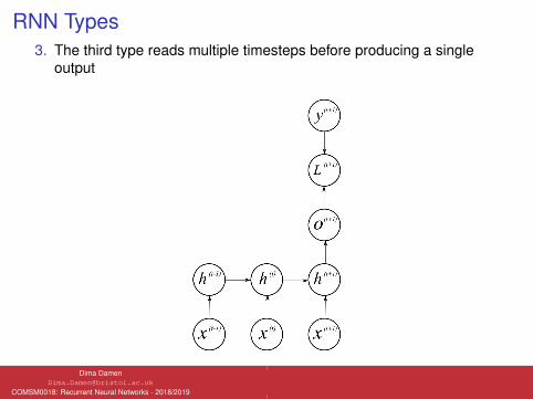
RNN Types3. The third type reads multiple timesteps before producing a single

output



RNN TypesI The left model can be used to learn any function computable with a

Turing machineI The middle model is less powerful. The information captured by the

output o is the only information it can send to the future. Unless o isvery high-dimensional and rich, it will lack important information fromthe past.

I The right model can be used to produce summaries (e.g.classifications of full sentences)



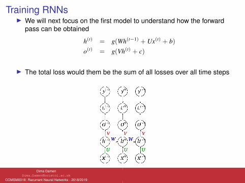
Training RNNsI We will next focus on the first model to understand how the forward

pass can be obtained

h(t) = g(Wh(t−1) + Ux(t) + b)

o(t) = g(Vh(t) + c)

I The total loss would them be the sum of all losses over all time steps



Training RNNs

I However, computing the gradient of this function is expensiveI It requires performing a forward propagation pass of the unrolled

network, followed by backward propagation pass throughout timeI The runtime is O(τ) and cannot be reduced by parallelisation because

the forward pass is sequentialI All computations in the forward pass must be stored until reused

during the backward pass, making the memory cost O(τ) as wellI This back-propagation algorithm is called back-propagation through

time (BPTT)



Training RNNs

I Practically, computing the gradient through an RNN is straightforward.I The generalised back-propagation algorithm is applied to the unrolled

network.I For the network below, the parameters are: U,V,W, b, c,I The nodes indexed by t: x(t), o(t),L(t) as well as the hidden node h(t)



Training RNNs

I After the forward pass, gradient is first computed at the nodesimmediately preceding the final loss

∂L∂L(t) = 1

I We can then calculate the loss using softmax and cross-entropy, giventhe output o(t)

∂L∂o(t) =

∂L∂L(t)

∂L(t)

∂o(t) = y(t)i − 1i,y(t)

I We then work our way backwards, from the end of the sequence tothe start



Training RNNs

I Because the parameters are shared across many time steps,calculating the derivative might seem confusing

I Calculating the derivative ∇WL operator, should take into account thecontribution of W from all edges in the graph.

I To resolve this, we introduce copies of W at different time steps W(t)

I We then calculate the gradient at time step t to be ∇W(t)



Training RNNs

I For the five parameters c, b,V,W,U, the gradients are given by

∇cL =∑

t

∇o(t)L

∇bL =∑

t

(∂h(t)

∂b(t)

)T∇h(t)L

∇VL =∑

t

∑i

( ∂L∂o(t)

)T∇V(t)o(t)i =

∑t

(∇o(t)L)h(t)T

∇WL =∑

t

∑i

( ∂L∂h(t)

)T∇W(t)h(t)i =

∑t

diag(1− (h(t))2)(∇h(t)L)h(t−1)T

∇UL =∑

t

∑i

( ∂L∂h(t)

)T∇U(t)h(t)i =

∑t

diag(1− (h(t))2)(∇h(t)L)x(t)T



Other RNN Types

I Bi-directional RNNsI Encoder-Decoder Sequence-to-Sequence architectureI Gated RNNsI Long-Short Term Memory (LSTMs)



Bi-directional RNNs

I We might want the prediction y(t) to depend on the whole sequence,its past and future

I This is particularly of relevance to speech recognition, machinetranslation or audio analysis

I As the name suggests, bidirectional RNNs combine an RNN thatmoves forward through time, beginning from the start of the sequence,with another that moves backward through time, beginning from theend of the sequence.

I This allows the output unit o(t) to compute a representation thatdepends on both the past and the future, without specifying anyfixed-size window around t



Bi-directional RNNs

I A typical bidirectional RNN



Encoder-Decoder RNN

I Mapping a variable-length sequence to another variable-lengthsequence

I You can refer to c as the contextI The encoder reads the input, emitting the context - a function of its

hidden statesI The decoder writes the fixed-level output sequence

Goodfellow p384



Long-Term Dependencies

I All previously mentioned architectures are good at learning short-termdependencies, without specifying a fixed-length

I However, gradients propagated over longer time tend to either vanishor explode

I Even when attempting to resolve the problem, by selecting parameterspaces where the gradients do not vanish or explode, the problempersists

I The gradient of a long-term interaction will always have exponentiallysmaller magnitude than the gradient of a short-term interaction

I The most effective solution for long-term dependencies are gatedRNNs



Gated RNNs

I Gated RNNs are based on creating paths through timeI This is achieved through connection weights that change at each time

stepI This allows the network to accumulate information over a long

duration - often referred to as memoryI It also allows the network to forget old states when neededI Previous approaches attempted to set these accumulation and

forgetting gates manually, while gated RNNs attempt to learn todecide when to do that.

I One of the most popular gated RNNs are LSTMs



LSTM

I First proposed by Hochreiter and Schmidhuber in 1997

Google Scholars 2017



LSTM

I The Adding Problem

Hochreiter and Schmidhuber (1997). Long-Short Term Memory. Neural Computation



Two-slice LSTM FigureI LSTM looks significantly more complex than an RNN until you start

dissecting it



Two-slice LSTM FigureI Let’s first simplify by keeping a single timestamp and only its

dependencies h(t−1), c(t−1)



LSTM

I The ability to forget thepast is controlled by whatis rightly named, theforget gate f (t)

I The weight of the forgetgate is set to a valuebetween 0 and 1 using asigmoid function

f (t)i = σ

(bf

i +∑

j

Ufi,jx

(t)j +

∑j

W fi,jh

(t−1)j

)f (t) = bf + Uf x(t) + W f h(t−1)



LSTM

I The external input gateunit i is computed in thesame way as the forgetgate

I Again, its weight is set toa value between 0 and 1using a sigmoid function

i(t) = bi + Uix(t) + W ih(t−1)



LSTM

I The state gate unit c isthen updated as follows

I Where ◦ is anelement-wisemultiplication

c(t) = f i ◦ c(t−1) + i(t) ◦ σ(

bj + Ujx(t) + W jh(t−1))



LSTM

I The output gate unit oalso uses a sigmoidfunction

o(t) = σ(

bo + Uox(t) + Woh(t−1))



LSTM

I And finally

h(t) = tanh(c(t)) ◦ o(t)



Gated RNNs

I While LSTMs proved useful for both artificial and real data, questionswere asked on whether this level of complexity is necessary

I Recently, gated RNNs (GRUs) are increasingly used where a singlegating unit controls the forget factor and the update factor as follows,



Gated RNNsI An update gate

u(t) = σ(

bu + Uux(t) + Wuh(t))

I A reset gater(t) = σ

(br + Urx(t) + Wrh(t)

)I A single update equation

h(t)i = u(t−1)

i h(t−1)i +(1− u(t−1)

i )σ(

bi +∑

j

Ui,jx(t−1)j +

∑j

Wi,jr(t−1)j h(t−1)

j

)

I The reset gates chose to ignore parts of the state vectorI The update gates linearly gate any dimension, copying or completely

ignoring itI The reset gates control which parts of the state get used, introducing

an additional nonlinear effect in the relationship with the past state.



Further Reading

I Deep Learning

Ian Goodfellow, Yoshua Bengio, and Aaron CourvilleMIT Press, ISBN: 9780262035613.I Chapter 10 – Sequence Modeling: Recurrent and Recursive Nets



coms0018: recurrent neural networks - github pages › ...coms0018: recurrent neural networks dima...

Documents