computer vision and image understanding

Computer Vision and Image Understanding 116 (2012) 999–1013

Contents lists available at SciVerse ScienceDirect

Computer Vision and Image Understanding

journal homepage: www.elsevier .com/ locate/cviu

Scale-space texture description on SIFT-like textons q

Yong Xu a,⇑, Sibin Huang a,b, Hui Ji b, Cornelia Fermüller c

a School of Computer Science & Engineering, South China University of Technology, Guangzhou 510006, Chinab Department of Mathematics, National University of Singapore, Singapore 117543, Singaporec Institute for Advanced Computer Studies, University of Maryland, College Park, MD 20742, USA

a r t i c l e i n f o a b s t r a c t

Article history:Received 17 May 2011Accepted 14 May 2012Available online 24 May 2012

Keywords:TextureMulti-fractal analysisImage featureWavelet tight frame

1077-3142/$ - see front matter � 2012 Elsevier Inc. Ahttp://dx.doi.org/10.1016/j.cviu.2012.05.003

q This paper has been recommended for acceptance⇑ Corresponding author.

E-mail addresses: [email protected] (Y. Xu), [email protected] (H. Ji), [email protected] (C. Fer

Visual texture is a powerful cue for the semantic description of scene structures that exhibit a high degreeof similarity in their image intensity patterns. This paper describes a statistical approach to visual texturedescription that combines a highly discriminative local feature descriptor with a powerful global statis-tical descriptor. Based upon a SIFT-like feature descriptor densely estimated at multiple window sizes, astatistical descriptor, called the multi-fractal spectrum (MFS), extracts the power-law behavior of thelocal feature distributions over scale. Through this combination strong robustness to environmentalchanges including both geometric and photometric transformations is achieved. Furthermore, to increasethe robustness to changes in scale, a multi-scale representation of the multi-fractal spectra under a wave-let tight frame system is derived. The proposed statistical approach is applicable to both static anddynamic textures. Experiments showed that the proposed approach outperforms existing static textureclassification methods and is comparable to the top dynamic texture classification techniques.

� 2012 Elsevier Inc. All rights reserved.

1. Introduction

Visual texture has been found a powerful cue for characterizingstructures in the scene, which give rise to certain patterns that ex-hibit a high degree of similarity. Classically, static image texturewas used for classification of materials, such as cotton, leather orwood, and more recently it has been used also on unstructuredparts of the scene, such as forests, buildings, grass, trees or shelvesin a department store. Dynamic textures are video sequences ofmoving scenes that exhibit certain stationary properties in time,such as sequences of rivers, smoke, clouds, fire, swarms of birds,humans in crowds, etc. A visual texture descriptor becomes usefulfor semantic description and classification, if it is highly discrimi-native and at the same time robust to environmental changes[51]. Environmental changes can be due to a wide range of factors,such as illumination changes, occlusions, non-rigid surface distor-tions and camera viewpoint changes.

Starting with the seminal work of [21], static image texture hasbeen studied in the context of various applications [15,20]. Earlierwork was concerned with shape from texture (e.g. [1,16,28]), andmost of the recent works are about developing efficient texture rep-resentations for the purpose of segmentation, classification, or syn-thesis. There are two components to texture representations:

ll rights reserved.

by Tinne Tuytelaars.

[email protected] (S. Huang),müller).

statistical models and local feature measurements. Some widelyused statistical models include Markov random fields(e.g. [11,43]), joint distributions, and co-occurrence statistics (e.g.[22,23,36]). Local measurements range from pixel values over sim-ple edge responses to local feature descriptors and filter bank re-sponses (e.g. [7,19,24,25,30–32,43,46,47,49]).

Approaches employing sophisticated local descriptors usuallycompute as statistics various texton histograms based on someappearance based dictionary. Depending on the percentage of pixelinformation used in the description, these approaches can be clas-sified into two categories: dense approaches and sparse approaches.Dense approaches apply appearance descriptors to every pixel. Forexample, Varma et al. [43] used the responses of the MR8 filterbank, consisting of a Gaussian, a LOG filter and edges in differentdirections at a few scales. In contrast, sparse approaches employappearance-based feature descriptors at a sparse set of interestpoints. For example, Lazebnik et al. [24] obtained impressive re-sults by combining Harris and Laplacian keypoint detectors andRIFT and Spin image affine-invariant appearance descriptors. Boththe sparse and dense approaches have advantages and disadvan-tages. The sparse approaches achieve robustness to environmentalchanges because the features are normalized. However, they maylose some important texture primitives by using only a small per-centage of the pixels. Also, there are stability and repeatability is-sues with the keypoint detection of existing point or regiondetectors. By using all pixels, the dense approaches provide richinformation for local texture characterizations. However, on thenegative side, the resulting descriptions tend to be more sensitive

http://dx.doi.org/10.1016/j.cviu.2012.05.003

mailto:[email protected]




http://dx.doi.org/10.1016/j.cviu.2012.05.003

http://www.sciencedirect.com/science/journal/10773142

http://www.elsevier.com/locate/cviu

1000 Y. Xu et al. / Computer Vision and Image Understanding 116 (2012) 999–1013

to significant environmental changes, such as changes in view-point, that affect the local appearance of image pixels. To rectifythe local appearance, we would need adaptive region processes.Such processes, however, would require strong patterns in the lo-cal regions of image pixels, which are not available for most imagepoints. Thus, rectification, which is standard for sparse sets of im-age points, cannot be adapted for dense sets.

In addition to the static texture in single images, dynamic tex-ture analysis also considers a stochastic dynamic behavior in thetemporal domain. Chetverikov and Péteri [5] gave a brief surveyof methods on dynamic texture description and recognition. Earlierdynamic texture classification systems (e.g. [33,10,38,45]) oftenexplicitly modeled the underlying physical process, and then dis-tinguished different dynamic textures by the values of the associ-ated model parameters. For example, Doretto et al. [10] usedlinear dynamical system (LDS) to characterize dynamic texture pro-cesses. The LDSs of the different textures were then compared in aspace described by Stiefel manifolds using the Martin distance.Ghanem and Ahuja [18] introduced a phase-based model for dy-namic texture recognition and synthesis. Dynamic characteristicsof dynamic texture were measured in Fazekas and Chetverikov[13] using optical flow based statistical measurements. However,it appears that so far no universal physical process has been foundthat can model a large set of dynamic textures. Thus, recently,appearance based discriminative methods have become more pop-ular for dynamic texture classification [3,37,44,50]. Wildes andBergen [44] constructed spatiotemporal filters to qualitatively clas-sify local motion patterns into a small set of categories. Thedescriptor proposed by Zhao and Pietikäinen [50] is based on localspatio-temporal statistics, specifically an extension of the local bin-ary pattern (LBP) in 2D images to the 3D spatio-temporal volumes.To compare different descriptors efficiently the co-occurrence ofLBPs was computed in three orthogonal planes. Ravichandranet al. [37] combined local dynamic texture structure analysis andgenerative models. They first applied the LDS model to localspace-time regions and then constructed a bag-of-words modelbased on these local LDSs. Chan and Vasconcelos [3] used kernelPCA to learn a non-linear kernel dynamic texture and applied itfor video classification.

In order to achieve good robustness necessary for semantic clas-sification, both components of texture description, the localappearance descriptors and the global statistical characterization,should accommodate environmental changes. In the past, very ro-bust local feature descriptors have been developed, such as thewidely used SIFT feature [27] in image space. Most approachesmaking use of these feature points use histograms for global statis-tical characterization. However, such histograms are not invariantto global geometrical changes. Furthermore, important informa-tion about the spatial arrangement of local features is lost. Aninteresting statistical tool, the so-called MFS (multi-fractal spectra)was proposed in [47] as an alternative to the histogram. The advan-tage of the MFS is that it is theoretically invariant to any smoothtransform (bi-Lipschitz geometrical transforms), and it encodesadditional information regarding the regularization of the spatialdistribution of pixels. A similar concept was used also in other tex-ture applications, for example in texture segmentation [6]. In [47]the MFS was applied to simple local measurements, the so-calledlocal density function, and in [48] it was applied to wavelets.Although the MFS descriptor proposed in [47] has been demon-strated to have strong robustness to a wide range of geometricalchanges including viewpoint changes and non-rigid surfacechanges, its robustness to photometric changes is weak. The mainreason is that the local feature description is quite sensitive to pho-tometric changes. Moreover, the simple local measurements havelimited discriminative information. On the other hand, local fea-ture descriptors, such as SIFT [27], have strong robustness to pho-

tometric changes as has been demonstrated in many applications.In particular, the gradient orientation histogram used in SIFT andvariations of SIFT has been widely used in many recognition andclassification tasks including texture classification (e.g. [24]).

Here we propose a new statistical framework that combines theglobal MFS statistical measurement and local feature descriptorsusing the gradient orientation histogram. The new framework isapplicable to both static and dynamic textures. Such a combinationwill lead to a powerful texture descriptor with strong robustness toboth geometric and photometric variations. Fig. 1 gives an outlineof the approach for static image textures. First, the scale-invariantimage gradients are derived based on a modification of the scale-selection method introduced in [26]. Next, at every pixel multi-scale gradient orientation histograms are computed with respectto multiple window sizes. Then, using a rotation-invariant pixelclassification scheme defined on the orientation histograms, pixelsare categorized, and the MFS is computed for every window size.The MFSs corresponding to different window sizes together makeup an MFS pyramid. The final texture descriptor is derived by sam-pling the leading coefficients (that is, coefficients of large magni-tude) of the MFS pyramids under a tight wavelet frametransform [8].

The approach for dynamic textures is essentially the same asthat for static textures with the 2D image SIFT feature replacedby the 3D SIFT feature proposed in Scovanner et al. [40]. Our ap-proach falls in the category of appearance-based discriminative ap-proaches. Its main advantage stems from its close relationship tocertain stochastic self-similarities existing in a wide range of dy-namic processes capable of generating dynamic textures.

The rest of the paper is organized as follows. Section 2 gives abrief review of the basic tools used in our approach. Section 3 pre-sents the algorithm in detail, and Section 4 is devoted to experi-ments on static and dynamic texture classification. Section 5concludes the paper.

2. Preliminaries: multi-fractal analysis

In this section, we give a brief review on multi-fractal analysis.A review on tight framelet systems is given in Appendix A. Multi-fractal analysis [12] is built upon the concept of the fractal dimen-sion, which is defined on point sets. Consider a set of points E in the2D image plane with same value of some attribute, e.g., the set ofimage points with same brightness. The fractal dimension of such apoint set E is a statistical measurement that characterizes how thepoints in E are distributed over the image plane when one zoomsinto finer scales. One definition of the fractal dimension, associatedwith a relatively simple numerical algorithm, is the so-called box-counting fractal dimension, which is as follows: Let the imageplane be covered by a square mesh of total n � n elements. Let# E; 1

n

� �be the number of squares that intersect the point set E.

Then the box-counting fractal dimension, denoted as dim(E), is de-fined as

dimðEÞ ¼ limn!1

log # E; 1n

� �� log 1

n

: ð1Þ

In other words, the box-counting fractal dimension dim(E) measuresthe power law behavior of the spatial distribution of E over the scale1/n:

# E;1n

� �/�1

n

��dimðEÞ:

In a practical implementation, the value of n is bounded by the im-age resolution, and dim(E) is approximated by the slope of the linefitted to

Fig. 1. Outline of the proposed approach.

Y. Xu et al. / Computer Vision and Image Understanding 116 (2012) 999–1013 1001

log # E;iN

� �with respect to � log

iN

for i ¼ 1;2; . . . ;m; m < N;

with N denoting the image resolution. In our implementation weuse the least squares method at points at i = 4, 5, 6, 7 to estimatethe slope.

Multi-fractal analysis generalizes the concept of the fractaldimension. One approach of applying multi-fractal analysis toimages is to classify the pixels in the image into multiple point setsaccording to some associated pixel attribute a. For each value of ain its feasible discretized domain, let E(a) be the collection of allpoints with the same attribute value a. The MFS of E then is definedas the vector dim(E(a)) vs a. In other words,

MFS ¼ ½dimðEða1ÞÞ;dimðEða2ÞÞ; . . . ; dimðEðanÞÞ�:

For example, in [47] the density function (a function describing thelocal change of the intensity over scale) was used as the pixel attri-bute. The density was quantized into n values, and then the fractaldimensions of n sets associated with these n values were concate-nated into a MFS vector.

3. Main components of the texture descriptor

Our algorithm, taking as input a static texture image, consists offour computational steps:

1. The first step is to calculate scale-invariant image gradients inthe scale-space of the texture image. At each point the scale isdetermined by the maximum of the Laplacian measure result-ing in a scale-invariant image gradient field.

2. Next, using as input the scale-invariant image gradient field, atevery pixel local orientation histograms are computed over mwindow sizes (m = 5 in our implementation). Similar as in theSIFT feature approach, we use 8 directions in the orientationhistogram. Two types of orientation histogram are used: onesimply counts the number of edges in each direction and theother uses the summation of edge energy in each direction.Thus, in total we obtain 2⁄m sets of local orientation histogramsfor the given image.

3. Then the MFS pyramid is computed. The orientation histogramsare discretized into n (n = 29 in our implementation) classesusing rotation-invariant templates, and an MFS vector is com-puted on this classification. We then combine the m MFS vec-tors corresponding to the m window sizes into an MFSpyramid. At the end of this step, we have 2 MFS pyramids of sizem � n.

4. Finally, a sparse tight framelet coefficient vector of each MFSpyramid is estimated, by keeping only the frame coefficientsof largest magnitude and setting to 0 all others.

The algorithms for static texture images and dynamic texturesequences are similar, but a SIFT-type descriptor in 2D image spaceis used in the former case and a SIFT-type descriptor in 3D spatio-temporal volume (see [40]) in the latter. Next, we give a detaileddescription of every step described in the algorithm above.

3.1. Scale-invariant image gradient field

The texture measurement of the proposed method is built uponthe image gradients of the given image. To suppress variations ofimage gradients caused by possible scale changes, we computethe image gradients in scale-space. Given an image I(x,y), its linearscale-space L(x,y;r) is obtained by convolving I(x,y) with an isotro-pic Gaussian smoothing kernel of standard deviation r:

gðx; y; rÞ ¼ 12pr2 e

� x2þy2

2r2

� �; ð2Þ

such that

Lðx; y;rÞ ¼ ðgð�; �;rÞ � IÞðx; yÞ ð3Þ

with a sequence of r = {1, . . . ,K} ranging from 1 to K (K = 10 in ourimplementation). Then, at each pixel (x,y), its associated image gra-dient is calculated as

½@xLðx; y;r�ðx; yÞÞ; @yLðx; y; r�ðx; yÞÞ�

for a particular standard deviation r⁄(x,y). The value r⁄(x,y) isdetermined by the scale selection method proposed in [26] whichselects at every point the scale at which some image measurement


takes on the extreme value. We use the Laplacian measurement, de-fined as

ML ¼ r4 Lx2 þ Ly2

� �ð4Þ

with Lxmyn ðx; y;rÞ ¼ @xmyn ðLðx; y; rÞÞ. In our implementation, the Pre-witt filters are used for computing the partial derivatives in scale-space. Then, the scale is derived by taking the maximum value ofthe Laplacian measurement over scale. The gradient magnitudeand orientation are computed by applying the finite differenceoperator to L(x,y;r⁄). See Fig. 2 for an illustration of the scale se-lected at each pixel and the corresponding image gradients.

3.2. Multi-scale local orientation histograms

Our proposed local feature descriptor relies on the local orienta-tion histogram of image pixels, which also is used in SIFT [27] andsimilar features. Its robustness to illumination changes and invari-ance to in-plane rotations has been demonstrated in many applica-tions. For each image gradient field computed in the previous step,at every pixel, two types of local orientation histograms are com-puted. One simply counts the number of orientations; the otherweighs them by the gradient magnitude. The gradient orientationsare quantized into 8 directions, covering 45 degrees each. To cap-ture information of pixels in a multi-scale fashion, for each pixel,we compute the orientation histograms at 5 window sizes rangingfrom 3 � 3 to 11 � 11. The orientation histograms, as in SIFT, arerotated to align the dominant orientation with a canonicaldirection.

3.3. Pixel classification and the MFS

The next step is to compute the MFS vector. The MFS vector de-pends on how the pixels are classified. To obtain a reasonable sta-

(a) Sample texture region (b) Scale

Fig. 2. (a) Sample texture region. (b) Selected scale r⁄ based on the maximum of the Lapimage gradient field, where the circle at a point denotes the size of the Gaussian smoot

(a)Fig. 3. (a) Representative elements for each of the 29 classes of orientation histogram teobtained from the possible mirror-reflections and rotations of the basic element.

tistics of the spatial distribution of pixels, the number of pixels ineach class needs to be sufficiently large. We thus need a meaning-ful way of discretizing the very large amount of possible orienta-tion histograms. Our approach is to introduce a fixed binpartitioning scheme based on a set of basic orientation histogramtemplates.

First, the estimated orientation histograms are quantized as fol-lows. For each bin the value is set to 0 if the magnitude is less than18 of the overall magnitude and to 1 otherwise. We then define apartitioning scheme based on the topological structure of orienta-tion histograms, with a total of 29 classes. See Fig. 3a and b for anillustration. The proposed templates are defined on the basis of thenumber of significant image gradient orientations and their rela-tive positions. Each template class contains the basic elementshown in Fig. 3a and all of its rotated and mirror-reflected copiesas shown in Fig. 3b for one of the elements.

Next, for each window size the corresponding MFS feature vec-tor is calculated as follows: For each template class (out of 29 clas-ses), a binary image is derived by setting the value of the pixel to 1if its associated template falls into the corresponding templateclass and to 0 otherwise (see Fig. 4). Thus, there are 29 binaryimages. For each binary image the box-counting fractal dimensionis computed, and the fractal dimensions are concatenated into a29-dim MFS vector. The MFS feature vectors corresponding to dif-ferent window sizes are then combined into a multi-scale MFS pyr-amid. The size of this MFS pyramid is 5 � 29.

It is noted that the box-counting fractal dimension amounts tofitting the slope of the line in the co-ordinate space of log # E; i

N

� �vs. � log i

N. Thus, the validity of the MFS largely depends on howapplicable such linearity assumption is for the given data. In ourapplication we used four points only (corresponding to four win-dow sizes) in the computation, and we found the variance in thefitting reasonably small to justify the fitting. Fig. 5a and b (the forth

(c) Image gradient0

2

4

6

8

10

lacian measure in scale-space with the scale ranging from 1 to 10. (c) Correspondinghing kernel (defined by r⁄) when computing the gradient.

(b)mplates. (b) All the elements in one orientation histogram template class, which are

Fig. 4. (a) Two texture images in UIUC dataset [27]. (b)–(e) Examples of binary images with respect to pixel classification based on the orientation histogram templates.

2 4 6 8 104

6

8

10

12

14

16

2 4 6 8 104

6

8

10

12

14

16

2 4 6 8 104

6

8

10

12

14

16

2 4 6 8 104

6

8

10

12

14

16

0 20 40 60 80 100 120 1400

0.5

1

1.5

2

0 20 40 60 80 100 120 1400

0.5

1

1.5

2

0 20 40 60 80 100 120 1400

0.5

1

1.5

2

0 20 40 60 80 100 120 1400

0.5

1

1.5

2

Fig. 5. Illustration of the MFS and the linear fitting behavior when computing the fractal dimensions for 2 static texture classes in (a, b) and 2 dynamic texture classes in (c, d).The sample static textures are from the UMD dataset [47], and the sample dynamic textures are from Ref. [9]. For each class, the first three rows show three sample statictexture images, or key frames of three sample dynamic textures. The forth row shows for one particular orientation histogram template, the graph of linear fitting in the co-ordinates of log # E; i

N

� �vs. � log i

N ; i ¼ 4; . . . ;7. The mean variances of the line fitting were found as 0.05, 0.11, 0.01 and 0.04 respectively. The fifth row shows the MFSpyramids (as vectors) of the corresponding texture images and dynamic texture sequences.



row) illustrate the behavior of the linear fitting in log-log coordi-nates for three images, each from two of the classes in the UMDdataset [47], which represent one of the best and one of the worstcases in the set, with variances of 0.05 and 0.11, respectively. Thelast row in Fig. 5 illustrates the corresponding MFSs. As can beseen, both for (a) and (b), the MFS pyramids of the three texturesare almost the same, demonstrating that the MFS descriptor cap-tures well the identity of texture classes.

It is easy to see that the orientation histogram templates pro-vide a pixel classification scheme which is invariant to rotationand mirror-reflection; in addition, the robustness to illuminationchanges is guaranteed by the orientation histogram itself [27].Using the MFS as the replacement of the histogram for statisticalcharacterization leads to better robustness to global geometricchanges (see [47] for more details).

3.4. Robustifying the texture descriptor in the wavelet frame domain

The final step is to construct the texture descriptor by only takingthe leading coefficients of the MFS pyramids in a wavelet frame do-main. The purpose is to further increase the robustness of the texturedescriptor to environmental changes. The construction is done asfollows: We first decompose the MFS pyramid using the 1D un-dec-imal linear-spline framelet transform [8], as it has been empiricallyobserved that the corresponding tight frame coefficients tend to behighly relevant to the essential structure of textures.

Let the matrix E(s,n) denote the MFS pyramid where s denotesthe scale (window size of local orientation histogram) and n de-notes the index of the template class. Let F denote the L-leveldecomposition of E(s,n) under a 1D tight framelet system with re-spect to s defined as

Fðj; s;nÞ :¼ AEðs;nÞ;

where A is the frame decomposition operator, and j denotes the le-vel of the frame decomposition. See Appendix A for more details onthe frame decomposition operator A. The multi-dimensional matrixF consists of two kinds of components: one low-pass framelet coef-ficient component H0, the output of applying the low-pass h0 on thepyramid at scale 2�L; and multiple high-pass framelet coefficientcomponents H1, . . ., Hr, the outputs of applying high pass filtersh1, . . ., hr to the pyramid at multiple levels ranging from 2�1, . . .,

Orig

inal

MFS

Glass Feature Sample

5 10 15 20 25

2468

10

H0

5 10 15 20 25

2468

10

H1

5 10 15 20 25

2468

10

H2

5 10 15 20 25

2468

10

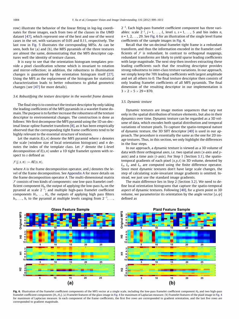
(a)Fig. 6. Illustration of the framelet coefficient components of the MFS vector at a singleframelet coefficient components {H1,H2}. (a) Framelet features of the glass image in Fig. 4for maximum of Laplacian measure. In each component of the frame coefficients, the ficorresponded to gradient magnitude.

2�L. Each high-pass framelet coefficient component has three vari-ables: scale 2�j, j = 1, . . ., L, level s, s = 1, . . ., 5 and bin index n,n = 1, 2, . . ., 29. See Fig. 6 for an illustration of the single level framecoefficients of the sample images in Fig. 4.

Recall that the un-decimal framelet tight frame is a redundanttransform, and thus the information encoded in the framelet coef-ficients of F is redundant. In contrast to orthogonal mappings,redundant transforms are likely to yield sparse leading coefficientswith large magnitude. The next step then involves extracting theseleading coefficients such that the resulting descriptor providesstrong robustness to inter-class texture variations. In our approach,we simply keep the 70% leading coefficients with largest amplitudeand set all others to 0. The final texture descriptor then consists ofonly leading framelet coefficients of all MFS pyramids. The finaldimension of the resulting descriptor in our implementation is3 � 2 � 5 � 29 = 870.

3.5. Dynamic texture

Dynamic textures are image motion sequences that vary notonly in the spatial distribution of texture elements, but also in theirdynamics over time. Dynamic texture can be regarded as a 3D vol-ume of data, which encodes both spatial distribution and temporalvariations of texture pixels. To capture the spatio-temporal natureof dynamic texture, the 3D SIFT descriptor [40] is used in our ap-proach. The procedure is essentially the same as the one for 2D im-age textures. Thus, in this section, we only highlight the differencesin the four steps.

In our approach, a dynamic texture is viewed as a 3D volume ofdata with three orthogonal axes, i.e. two spatial axes (x-axis and y-axis) and a time axis (t-axis). For Step 1 (Section 3.1), the spatio-temporal gradients of each pixel (x,y, t) in 3D volume, denoted byLx, Ly and Lt, are computed using the finite difference operator.Since most dynamic textures don’t have large scale changes, thestep of calculating scale-invariant image gradients is omitted. In-stead, we just use the standard image gradients.

The main difference lies in Step 2 (Section 3.2). We need to de-fine local orientation histograms that capture the spatio-temporalaspect of dynamic textures. Following [40], for a given point in 3Dvolume, we parameterize its orientation by the angle vector [/,w]defined as

Orig

inal

MFS

Plaid Feature Sample

5 10 15 20 25

2468

10

H0

5 10 15 20 25

2468

10

H1

5 10 15 20 25

2468

10

H2

5 10 15 20 25

2468

10

(b)scale, including the low-pass framelet coefficient component H0 and two high-passfor maximum of Laplacian measure. (b) Framelet features of the plaid image in Fig. 4rst five rows are corresponded to gradient orientation, and the last five rows are

(a) 25 sample static textures from the UIUC dataset.

(b) 25 sample static textures from the UMD dataset.

Fig. 7. Sample static texture images.



/ ¼ tan�1 Ly

Lx

w ¼ tan�1 LtffiffiffiffiffiffiffiffiffiL2

xþL2y

p ;

8<:

with the two angles ranging from 0� to 360�. To reduce the compu-tational cost, we only use the orientation variable w in the orienta-tion histogram templates. This variable captures the temporalinformation of dynamic textures. Using the orientation histogramtemplates described in Section 3.2 with respect to w, we obtainthe orientation histograms for the 3D volume data. The procedureof computing dynamic texture descriptor is as follows.

1. For each pixel, we compute the orientation histograms withrespect to parameter w at 5 windows (3D cubes) ranging in sizefrom 3 � 3 � 3 to 11 � 11 � 11. For each scale, we compute twotypes of local orientation histograms, one based on the numberof orientations, the other based on the gradient magnitude.

2. Then we classify the volumetric windows into 29 classes basedon the 29 orientation histogram templates described inSection 3.2.

3. Based on this classification we calculate using the 3D box-count-ing fractal dimension (1) the MFS vectors, and concatenate theMFS feature vectors of different window sizes into a multi-scaleMFS pyramid.

It is noted that the last step used in the computation of statictextures (Section 3.3) is not used here, as it leads to very minorimprovements in the classification experiments. The final dimen-sion of the 3D dynamic texture descriptor is 2 � 5 � 29 = 290.Fig. 5c and d illustrate the estimated MFS and the fitting of the linefor one 3D orientation histogram template on a good and a bad

5 10 15 2060

70

80

90

100

Number of training samples

Cla

ssifi

catio

n ra

te

LaplacianLaplacian+Frame

Fig. 8. Comparison of the average classification rates vs. number of training samples ofwas run on the UMD dataset using SVM classification.

0 5 10 15 200.6

0.7

0.8

0.9

1


Cla

ssifi

catio

n ra

te

(H+L)(S+R)MFSVG−fractalOTF

1 0 5 10.4

0.5

0.6

0.7

0.8

0.9

1

Number of tr

Cla

ssifi

catio

n ra

te

1

(a) (bFig. 9. Classification rate vs. number of training samples for the UIUC dataset based on Set al. [24], the MFS method in Xu et al. [47], the VG-Fractal method in Varma et al. [42] arate for all 25 classes. (c) Classification rate of the worst class.

case, demonstrating the variance sufficiently small to justify thelinearity assumption in the estimation of the fractal dimension.

4. Experimental evaluation

The performance of the proposed texture descriptor is evalu-ated for static and dynamic texture classification. All code is avail-able at [52].

4.1. Static texture

We evaluated the performance of texture classification on twodatasets, the UIUC dataset [27] and the high-resolution UMD data-set [47]. Sample images of these datasets are shown in Fig. 7. TheUIUC texture dataset consists of 1000 uncalibrated and unregis-tered images: 40 samples for each of 25 textures with a resolutionof 640 � 480 pixels. The UMD texture dataset also consists of 1000uncalibrated and unregistered images: 40 samples for each of 25textures with a resolution of 1280 � 900 pixels. In both datasetssignificant viewpoint changes and scale differences are present,and the illumination conditions are uncontrolled.

In our experiments, the training set is selected as a fixed sizerandom subset of the class, and all remaining images are used asthe test set. A final texture description is based on a two-scaleframelet-based representation. The reported classification rate isthe average over 200 random subsets. An SVM classifier [4,41] isused, which was implemented as in Pontil et al. [35]. The featuresof the training set are used to train the hyperplane of the SVM clas-sifier using RBF kernels as described in Scholkopf et al. [39]. Theoptimal parameters are discovered by cross-validation.

14 16 18 2097

97.5

98

98.5


Cla

ssifi

catio

n ra

te

LaplacianLaplacian+Frame

the proposed descriptor with and without wavelet robustification. The experiment

0 15 20aining samples


0 5 10 15 200

0.2

0.4

0.6

0.8

1


Cla

ssifi

catio

n ra

te


1

) (c)VM classification. Four methods are compared: the (H+L)(S+R) method in Lazebniknd our OTF method. (a) Classification rate for the best class. (b) Mean classification


The approach was implemented in Matlab 2011b and run on alaptop computer with Intel Core 2 Duo with 2.10 GHz and 4 GBmemory. For each image in the UIUC dataset, the running time ofthe proposed feature extraction is about 10 s. Since our proposedapproach does not require expensive clustering, the classificationis very efficient. The average running time is around 16 s for clas-sifying 750 images of 25 classes from the UIUC dataset using theSVM-based classifier with 10 training samples for each class.

To understand the influence of applying the wavelet transformon feature vectors, we compared the average classification rates of

0 10 200

20

40

60

80

10097.02

Cla

ssifi

catio

n ra

te (%

)

The Nth class of UIUC dataset

0 10 200

20

40

60

80

10092.31

Cla

ssifi

catio

n ra

te (%

)


(a)

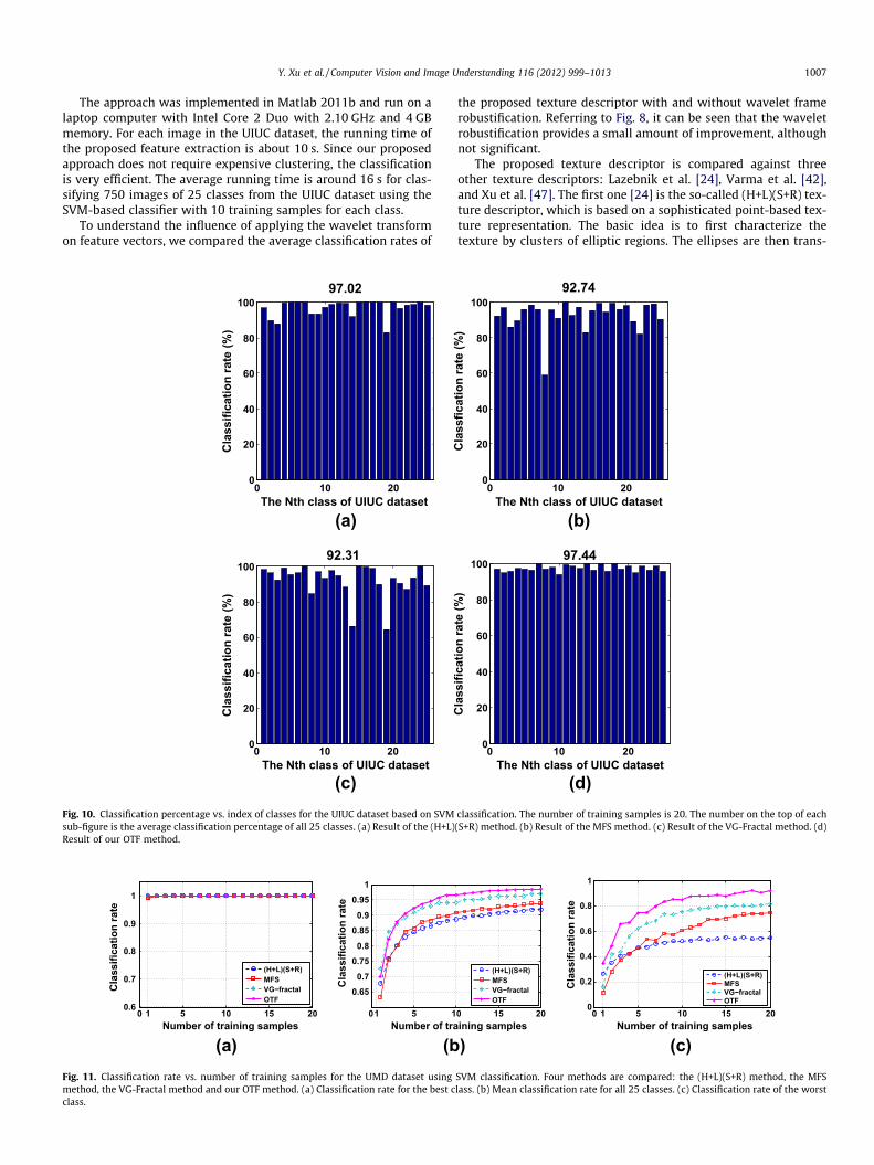
(c)Fig. 10. Classification percentage vs. index of classes for the UIUC dataset based on SVMsub-figure is the average classification percentage of all 25 classes. (a) Result of the (H+L)Result of our OTF method.

0 5 10 15 200.6

0.7

0.8

0.9

1


Cla

ssifi

catio

n ra

te


1 0 5 1

0.650.7

0.750.8

0.850.9

0.951

Number of tra

Cla

ssifi

catio

n ra

te

1

(b(a)Fig. 11. Classification rate vs. number of training samples for the UMD dataset usingmethod, the VG-Fractal method and our OTF method. (a) Classification rate for the best cclass.

the proposed texture descriptor with and without wavelet framerobustification. Referring to Fig. 8, it can be seen that the waveletrobustification provides a small amount of improvement, althoughnot significant.

The proposed texture descriptor is compared against threeother texture descriptors: Lazebnik et al. [24], Varma et al. [42],and Xu et al. [47]. The first one [24] is the so-called (H+L)(S+R) tex-ture descriptor, which is based on a sophisticated point-based tex-ture representation. The basic idea is to first characterize thetexture by clusters of elliptic regions. The ellipses are then trans-

0 10 200

20

40

60

80

10092.74

Cla

ssfic

atio

n ra

te (%

)


0 10 200

20

40

60

80

10097.44


Cla

ssifi

catio

n ra

te (%

)

(b)

(d)classification. The number of training samples is 20. The number on the top of each(S+R) method. (b) Result of the MFS method. (c) Result of the VG-Fractal method. (d)

0 15 20ining samples


0 5 10 15 200

0.2

0.4

0.6

0.8

1


Cla

ssifi

catio

n ra

te


1

(c))SVM classification. Four methods are compared: the (H+L)(S+R) method, the MFSlass. (b) Mean classification rate for all 25 classes. (c) Classification rate of the worst


formed to circles such that the local descriptor is invariant to affinetransforms. Two descriptors (SPIN and SIFT) are defined on each re-gion. The resulting texture descriptor is the histogram of clusters ofthese local descriptors, and the descriptors are compared using the

0 10 200

20

40

60

80

10096.95

Cla

ssifi

catio

n ra

te (%

)

The Nth class of UM dataset

0 10 200

20

40

60

80

10096.36

Cla

ssifi

catio

n ra

te (%

)


(a)

(c)Fig. 12. Classification percentage vs. index of classes for the UMD dataset based on SVMsub-figure is the average classification percentage of all 25 classes. (a) (H+L)(S+R) meth

Fig. 13. Samples images from the dyna

EMD distance. The second method is the VG-fractal method byVarma and Garg [42], which uses properties of the local densityfunction of various image measurements resulting in a 13 dimen-sional descriptor. The resulting texture descriptor is the histogram

0 10 200

20

40

60

80

10093.93


Cla

ssifi

catio

n ra

te (%

)

0 10 200

20

40

60

80

10098.42


Cla

ssifi

catio

n ra

te (%

)(b)

(d)classification. The number of training samples is 20. The number on the top of each

od. (b) MFS method. (c) VG-fractal method. (d) OTF method.

mic textures in the DT-9 dataset.

Table 1Classification results (in %) for the UCLA dataset. Note: Superscript ‘‘M’’ is used to denote results using maximum margin learning (followed by 1NN) [17]; ‘‘–’’ means ‘‘notavailable’’. Boldface print is used to mark the best results.

Method DT-7 DT-8 DT-9 DT-50 DT-SIR

Classifier 1NN SVM 1NN SVM 1NN SVM 1NN SVM 1NN

[37] – – 70.00 80.00 – – – – –[9] 92.30 – – – – – 81.00 – 60.00[17] – – – – 95.60M – 99.00M – –3D-OTF 96.11 98.37 95.80 99.50 96.32 97.23 99.25 87.10 67.45

10 20 30 40 50

10

20

30

40

500

20

40

60

80

100

0 10 20 30 40 500

20

40

60

80

10099.25

10 20 30 40 50

10

20

30

40

500

20

40

60

80

100

0 10 20 30 40 500

20

40

60

80

10087.10

Fig. 14. Confusion matrices for DT-50 for classification. The upper is using a NN classifier, and the lower is using an SVM classifier.

10 20 30 40 50

10

20

30

40

500

20

40

60

80

100

0 10 20 30 40 500

20

40

60

80

10067.45

Fig. 15. Confusion matrix for DT-SIR for classification using NN classifier.


of clusters of these local descriptors. The third method, the MFSmethod by Xu et al. [47], derives the MFSs of simple local measure-ments (the local density function of the intensity, image gradientand image Laplacian). The texture descriptor is a combination ofthe three MFSs. The results on the UIUC dataset using the SVMclassifier for the (H+L)(S+R) method is from [24]. The other results

are obtained from our implementations. We denote our approachas OTF method. Fig. 9 shows the classification rate vs. the numberof training samples on the UIUC dataset. Fig. 10 shows the classifi-cation percentage vs. the index of classes on the UIUC datasetbased on 20 training samples. Figs. 11 and 12 show the results ofthe UMD dataset using the same experimental evaluation.

boiling water fire flowers foutains plants sea smoke water waterfall

boiling water

fire

flowers

foutains

plants

sea

smoke

water

waterfall

96.75

0.2

1.65

0.13

1.12

0.15

0.05

97.51

0.44

0.33

1.67

95.47

4.53

0.01

92.08

4.52

3.39

0.09

0.98

0.47

98.46

100

11.97

88.03

100 1.4

98.6

boiling water fire flowers foutains sea smoke water waterfall

boiling water

fire

flowers

foutains

sea

smoke

water

waterfall

96.5

1.1

0.7

0.2

1.5

96.42

0.4

3.18

100 1.3

94.94

0.02

3.74

100

6

6.45

80.15

4.8

2.6

100

0.11

1.44

98.45

flames fountain smoke turbulence waves waterfall vegetation

flames

fountain

smoke

turbulence

waves

waterfall

vegetation

90.35

9.2

0.2

0.25

100

4.75

87.15

0.5

7.6

98.4

1.36

0.24

0.13

99.86

0.01

0.65

0.55

1.76

97.04

100

boiling water fire flowers foutains plants sea smoke water waterfall

boiling water

fire

flowers

foutains

plants

sea

smoke

water

waterfall

95

3.75

1.25

100

86.67

13.33

2

96

2

0.09

99.91

100

97.5

2.5

100

100

boiling water fire flowers foutains sea smoke water waterfall

boiling water

fire

flowers

foutains

sea

smoke

water

waterfall

100

100

100

96

4

100

100

100

100

flames fountain smoke turbulence waves waterfall vegetation

flames

fountain

smoke

turbulence

waves

waterfall

vegetation

96.25

1.25

2.5

100

100

96.5

3.5

99.92

0.08

0.93

3.13

95.94

100

(a) DT-9:NN (b) DT-8:NN (c) DT-7:NN

(d) DT-9:SVM (e) DT-8:SVM (f) DT-7:SVM

Fig. 16. Confusion matrices for UCLA DT-9, DT-8 and DT-7 for classifications, the upper is using NN classifier, and the lower is using SVM classifier.

Table 2Results in leave-one-group-out test (%) on DynTex dataset.

LBP-TOP [50] 3D-OTF

Non-weighting 95.71 95.89Best-weighting 97.14 96.70


From Fig. 9–12, it is seen that our method clearly outperformedthe VG-fractal method and the MFS method on both datasets. Alsoour method obtained better results than the (H+L)(S+R) method.We emphasize that heavy clustering is needed in both, the VG-fractal method and the (H+L)(S+R) method, which is very computa-tionally expensive. In contrast, our approach is much simpler andefficient without requiring clustering.

4.2. Dynamic texture

There are three public dynamic texture datasets that have beenwidely used: the UCLA dataset [10], the DynTex dataset [34] andthe DynTex++ dataset [17]. We applied our dynamic texture

10 20 30

5

10

15

20

25

30

350

20

40

60

80

100

Fig. 17. Confusion matrices by our method 3D-OTF on

descriptor for dynamic texture classification on these three data-sets and compared the results with those from a few state-of-the-art dynamic texture classification approaches.

4.2.1. UCLA datasetA popular dynamic texture benchmark for performance evalua-

tion is the UCLA dataset (e.g. [9,17,38,37,45]). The original UCLAdataset consists of 50 dynamic textures. Each dynamic texture isgiven in terms of four grayscale image sequences captured fromthe same viewpoint, resulting in a total of 200 sequences, each ofwhich consists of 75 frames of size 110�160. The literature doesnot agree on a ground truth regarding the classification of the UCLAdataset. In [9,17,37] the following five classifications, termed DT-50, DT-SIR, DT-9, DT-8 and DT-7, were considered:

1. DT-50 [9,17]. All 50 classes are used for classification.2. DT-SIR (Shift-invariant recognition) [9]. Each of the original 200

video sequences is spatially cut into non-overlapping, left andright halves resulting in a total of 400 sequences. The ‘‘shift-

10 20 30

5

10

15

20

25

30

35

the DynTex (left) and DynTex++(right) datasets.

100 91.5 90.5 100 89 100 88.5

78.5 100 100 100 79 100 100

100 100 100 100 100 100 100

99 93.5 100 86.5 100 85.5 100

74.5 100 100 100 100 100 100

Fig. 18. Classification rate (in %) for the different classes of the DynTex dataset.

Table 3Results (%) on DynTex++dataset.

Method DL-PEGASOS [17] 3D-OTF

Classification rate 63.70% 89.17%


invariant recognition’’ was used to eliminate the effects due tobiases in identical viewpoint selection. Nearest-neighbor classi-fication was applied in the recognition process.

3. DT-9 [17]. The dataset is divided into 9 classes: boiling water(8), fire (8), flowers (12), fountains (20), plant (108), sea (12),smoke (4), water (12) and waterfall (16), where the numberin parentheses denotes the number of elements of each class.Sample frames are shown in Fig. 13. In our experiments we usedthe original images of size 110⁄160.

100 100 92 100 86 78

94 98 100 100 96 98

98 28 24 100 86 100

Fig. 19. Classification rate (in %) for the dif

4. DT-8 [37]. This dataset is obtained from DT-9 by discarding thelarge class ‘‘plants’’, and considering only the eight otherclasses.

5. DT-7 [9] The original sequences in the dataset are split spatiallyinto left and right halves resulting in 400 sequences, whichwere classified into seven semantic categories: flames (16),fountain (8), smoke (8), turbulence (40), waves (24), waterfall(64) and vegetation (240).

We compared our method using both NN(Nearest-neighbor)and SVM classifiers to the methods in [9,17] and [37] on the fivecategorizations (DT-7, DT-8, DT-9, DT-50 and DT-SIR). See Table 1for a comparison of these methods. As can be seen from Table 1 ourmethod outperformed the other three state-of-the-art methods.We also included the so-called confusion matrix to show the details

100 96 60 100 100 82

100 100 100 100 94 94

100 82 86 64 100 74

ferent classes of the DynTex++dataset.

φ ψ1 ψ2

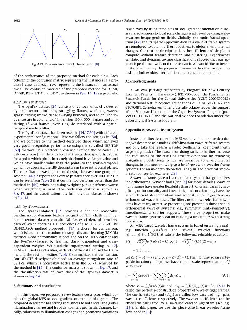
Fig. A.20. Piecewise linear wavelet frame system [8].


of the performance of the proposed method for each class. Eachcolumn of the confusion matrix represents the instances in a pre-dicted class and each row represents the instances in an actualclass. The confusion matrices of the proposed method for DT-50,DT-SIR, DT-9, DT-8 and DT-7 are shown in Figs. 14–16 respectively.

4.2.2. DynTex datasetThe DynTex dataset [34] consists of various kinds of videos of

dynamic texture, including struggling flames, whelming waves,sparse curling smoke, dense swaying branches, and so on. The se-quences are in color and of dimension 400 � 300 in space and con-sisting of 250 frames (over 10 s) de-interlaced with a spatio-temporal median filter.

The DynTex dataset has been used in [14,17,50] with differentexperimental configurations. Here we follow the settings in [50],and we compare to the method described there, which achievedvery good recognition performance using the so-called LBP-TOP[50] method. This method in essence extends the so-called 2DLBP descriptor (a qualitative local statistical descriptor, that codesfor a point which pixels in its neighborhood have larger value andwhich have smaller value than the point) to the spatio-temporaldomain by applying the LBP descriptors in three orthogonal planes.The classification was implemented using the leave-one-group-outscheme. Table 2 reports the average performance over 2000 runs. Itcan be seen from Table 2 that our method performs better than themethod in [50] when not using weighting, but performs worsewhen weighting is used. The confusion matrix is shown inFig. 17, and the classification rate for individual classes is shownin Fig. 18.

4.2.3. DynTex++datasetThe DynTex++dataset [17] provides a rich and reasonable

benchmark for dynamic texture recognition. This challenging dy-namic texture dataset contains 36 classes of dynamic textures,each of which contains 100 sequences of size 50 � 50 � 50. TheDL-PEGASOS method proposed in [17] is chosen for comparison,which is based on the maximum margin distance learning (MMDL)method. Good performance is obtained on the UCLA dataset andthe DynTex++dataset by learning class-independent and class-dependent weights. We used the experimental setting in [17].SVM was used as a classifier, with 50% of the dataset used for train-ing and the rest for testing. Table 3 summarizes the comparison.Our 3D-OTF descriptor obtained an average recognition rate of89.17%, which is noticeably better than the 63.7% achieved bythe method in [17]. The confusion matrix is shown in Fig. 17, andthe classification rate on each class of the DynTex++dataset isshown in Fig. 19.

5. Summary and conclusions

In this paper, we proposed a new texture descriptor, which ap-plies the global MFS to local gradient orientation histograms. Theproposed descriptor has strong robustness to both local and globalillumination changes and is robust to many geometric changes. Lo-cally, robustness to illumination changes and geometric variations

is achieved by using templates of local gradient orientation histo-grams; robustness to local scale changes is achieved by using scale-invariant image gradient fields. Globally, the multi-fractal spec-trum [47] and its sparse approximation in a wavelet frame systemare employed to obtain further robustness to global environmentalchanges. Our texture description is rather efficient and simple tocompute without feature detection and clustering. Experimentson static and dynamic texture classifications showed that our ap-proach performed well. In future research, we would like to inves-tigate how to apply the proposed framework to other recognitiontasks including object recognition and scene understanding.

Acknowledgments

Y. Xu was partially supported by Program for New CenturyExcellent Talents in University (NCET-10-0368), the FundamentalResearch Funds for the Central Universities (SCUT 2009ZZ0052)and National Nature Science Foundations of China 60603022 and61070091. Cornelia Fermüller gratefully acknowledges the supportof the European Union under the Cognitive Systems Program (pro-ject POETICON++) and the National Science Foundation under theCyberphysical Systems Program.

Appendix A. Wavelet frame system

Instead of directly using the MFS vector as the texture descrip-tor, we decompose it under a shift-invariant wavelet frame systemand only take the leading wavelet coefficients (coefficients withlarge magnitude). The reason for doing so is to further increasethe robustness of the resulting texture descriptor by removinginsignificant coefficients which are sensitive to environmentalchanges. In this section, we give a brief review on wavelet framesystems. For an in-depth theoretical analysis and practical imple-mentation, see for example [2,8].

A wavelet frame system is a redundant system that generalizesthe orthonormal wavelet basis (see [8] for more details). Wavelettight frames have greater flexibility than orthonormal bases by sac-rificing orthonormality and linear independence, but they have thesame efficient decomposition and reconstruction algorithms asorthonormal wavelet bases. The filters used in wavelet frame sys-tems have many attractive properties, not present in those used inorthonormal wavelet systems: e.g., symmetry (anti-symmetry),smoothness,and shorter support. These nice properties makewavelet frame systems ideal for building a descriptors with strongrobustness.

An MRA-based wavelet frame system is based on a single scal-ing function / 2 L2ðRÞ and several wavelet functionsfw1; . . . ;wrg � L2ðRÞ that satisfy the following refinable equation:

/ðtÞ ¼ffiffiffi2p X

k

h0ðkÞ/ð2t � kÞ; w‘ðtÞ ¼ffiffiffi2p X

k

h‘ðkÞ/ð2t � kÞ; ‘

¼ 1;2; . . . ; r:

Let /k(t) = /(t � k) and wk,j,‘ = w‘(2jt � k). Then for any square inte-grable function f 2 L2ðRÞ, we have a multi-scale representation of fas follows:

f ¼X1

k¼�1ck/kðtÞ þ

Xr

‘¼1

X1j¼0

X1k¼�1

dk;j;‘wk;j;‘; ðA:1Þ

where ck ¼R

Rf ðtÞ/kðtÞdt and dk;j;‘ ¼

RR

f ðtÞwk;j;‘ðtÞdt. Eq. (A.1) iscalled the perfect reconstruction property of wavelet tight frames.The coefficients {ck} and {dk,j,‘} are called low-pass and high-passwavelet coefficients respectively. The wavelet coefficients can beefficiently calculated by a so-called cascade algorithm (see e.g.[29]). In this paper, we use the piece-wise linear wavelet framedeveloped in [8]:


h0 ¼14½1;2;1�; h1 ¼

ffiffiffi2p

4½1;0;�1�; h2 ¼

14½�1;2;�1�:

See Fig. A.20 for the corresponding / and w1, w2. We follow [2] for adiscrete implementation of the multi-scale tight frame decomposi-tion without downsampling. For convenience of notation, we de-note such a linear frame decomposition by a rectangular matrix Aof size m � n with m > n. Thus, given any signal f 2 Rn, the discreteversion of (A.1) is expressed as follows:

f ¼ AT w ¼ ATðAfÞ;

where w 2 Rm is the wavelet coefficient vector of f. It is noted thatwe have ATA = I but AAT – I unless the tight framelet system degen-erates to an orthonormal wavelet system.

References

[1] J. Aloimonos, Shape from texture, Biological Cybernetics 58 (1988) 345–360.[2] J. Cai, R.H. Chan, Z. Shen, A framelet-based image inpainting algorithm, Applied

and Computational Harmonic Analysis 24 (2) (2008) 131–149.[3] A. Chan, N. Vasconcelos, Classifying video with kernel dynamic textures, CVPR

(2007).[4] Y.W. Chen, C.J. Lin, Combining SVMs with Various Feature Selection Strategies,

Feature Extraction, Foundations and Applications, Springer, 2006.[5] D. Chetverikov, R. Péteri, A brief survey of dynamic texture description and

recognition, in: Proc. 4th Int. Conf. on Computer Recognition Systems, SpringerAdvances in Soft Computing, 2005, pp. 17–26.

[6] A. Conci, L.H. Monterio, Multifractal characterization of texture-basedsegmentation, ICIP (2000) 792–795.

[7] K. Dana, S. Nayar, Histogram model for 3d textures, CVPR (1998) 618–624.[8] I. Daubechies, B. Han, A. Ron, Z. Shen, Framelets: MRA-based constructions of

wavelet frames, Applied and Computational Harmonic Analysis 14 (2003) 1–46.

[9] K.G. Derpanis, R.P. Wildes, Dynamic texture recognition based on distributionsof spacetime oriented structure, CVPR (2010).

[10] G. Doretto, A. Chiuso, Y.N. Wu, S. Soatto, Dynamic texture, IJCV (2003).[11] A. Efros, T. Leung, Texture synthesis by non-parametric sampling, ICCV (1999)

1039–1046.[12] K.J. Falconer, Techniques in Fractal Geometry, John Wiley, 1997.[13] S. Fazekas, D. Chetverikov, Analysis and performance evaluation of optical flow

features for dynamic texture recognition, in: Signal Processing: ImageCommunication, Special Issue on Content-Based Multimedia Indexing andRetrieval, vol. 22 (7–8), 2007, pp. 680–691,

[14] S. Fazekas, D. Chetverikov, Normal versus complete flow in dynamic texturerecognition: a comparative study, in: Workshop on Texture Analysis andSynthesis, 2005.

[15] D.A. Forsyth, J. Ponce, Computer Vision: A Modern Approach, Prentice Hall,2002.

[16] J. Garding, T. Lindeberg, Direct computation of shape cues using scale-adaptedspatial derivative operators, IJCV 17 (2) (1996) 163–191.

[17] B. Ghanem, N. Ahuja, Maximum margin distance learning for dynamic texturerecognition, ECCV (2010).

[18] B. Ghanem, N. Ahuja, Phase based modelling of dynamic textures, ICCV (2007).[19] E. Hayman, B. Caputo, M. Fritz, J.O. Eklundh, On the significance of real-world

conditions for material classification, ECCV (2004) 253–266.[20] D.J. Heeger, J.R. Bergen, Pyramid based texture analysis/synthesis, Computer

Graphics Proceedings (1995) 229–238.[21] B. Julesz, Texture and visual perception, Science America 212 (1965) 38–48.[22] C. Kervrann, F. Heitz, A Markov random field model-based approach to

unsupervised texture segmentation using local and global spatial statistics,IEEE Transactions on Image Processing 4 (6) (1995) 856–862.

[23] S.M. Konishi, A.L. Yuille, Statistical cues for domain specific imagesegmentation with performance analysis, CVPR (2000) 125–1132.

[24] S. Lazebnik, Local semi-local and global models for texture, object and scenerecognition, Ph.D. Dissertation, University of Illinois at Urbana-Champaign,2006.

[25] T. Leung, J. Malik, Representing and recognizing the visual appearance ofmaterials using three-dimensional texons, IJCV 43 (1) (2001) 29–44.

[26] T. Lindeberg, Automatic scale selection as a pre-processing stage forinterpreting the visual world, FSPIPA 130 (1999) 9–23.

[27] D. Lowe, Distinctive image features from scale invariant keypoints, IJCV 60 (2)(2004) 91–110.

[28] J. Malik, R. Rosenholtz, Computing local surface orientation and shape fromtexture for curved surfaces, IJCV 23 (2) (1997) 49–168.

[29] S. Mallat, A Wavelet Tour of Singapore Processing, third ed., The Sparse Way,Academic Press, 2008.

[30] B.B. Mandelbrot, The Fractal Geometry of Nature, Freeman, San Francisco, CA,1982.

[31] B.S. Manjunath, J.R. Ohm, V.V. Vasudevan, A. Yamada, Color and texturedescriptors, IEEE Transactions on Circuits and Systems for Video Technology11 (6) (2001) 703–715.

[32] F. Mindru, T. Tuytelaars, L. Van Gool, T. Moons, Moment invariants forrecognition under changing viewpoint and illumination, CVIU 94 (1–3) (2004)3–27.

[33] R.C. Nelson, R. Polana, Qualitative recognition of motion using temporaltexture, Computer Vision, Graphics, and Image Processing: ImageUnderstanding 56 (1) (1992) 78–89.

[34] R. Péteri, S. Fazekas, M.J. Huiskes, DynTex: a comprehensive database ofdynamic texture, Pattern Recognition Letters 31 (12) (2010) 1627–1632.

[35] M. Pontil, A. Verri, Support vector machines for 3D object recognition, PAMI 20(6) (1998) 637–646.

[36] J. Portilla, E.P. Simoncelli, A parametric texture model based on joint statisticsof complex wavelet coefficients, IJCV 40 (1) (2000) 49–71.

[37] A. Ravichandran, R. Chaudhry, R. Vidal, View-invariant dynamic texturerecognition using a bag of dynamical systems, CVPR (2009).

[38] P. Saisan, G. Doretto, Y. Wu, S. Soatto, Dynamic texture recognition, CVPR II(2001) 58–63.

[39] B. Scholkopf, A. Smola, Learning with Kernels: Support Vector Machines,Regularization, Optimization and Beyond, MIT Press, Cambridge, MA, 2002.

[40] P. Scovanner, S. Ali, M. Shah, A 3-dimensional SIFT descriptor and itsapplication to action recognition, ACM Multimedia (2007).

[41] V. Tresp, A. Schwaighofer, Scalable kernel systems, in: Proceedings of ICANN2001, Lecture Notes in Computer Science, vol. 2130, Springer Verlag, 2001, pp.285–291.

[42] M. Varma, R. Garg, Locally invariant fractal features for statistical textureclassification, ICCV (2007).

[43] M. Varma, A. Zisserman, Classifying images of materials: achieving viewpointand illumination independence, ECCV (2002) 255–271.

[44] R.P. Wildes, S.R. Bergen, Qualitative spatiotemporal analysis using an orientedenergy representation, ECCV (2000) 768–784.

[45] F. Woolfe, A. Fitzgibbon, Shift-invariant dynamic texture recognition, ECCV II(2006) 549–562.

[46] J. Wu, M.J. Chantler, Combining gradient and albedo for rotation invariantclassification of 2D surface texture, ICCV (2003) 848–855.

[47] Y. Xu, H. Ji, C. Fermuller, Viewpoint invariant texture description using fractalanalysis, IJCV 83 (1) (2009) 85–100.

[48] Y. Xu, X. Yang, H.B. Ling, H. Ji, A new texture descriptor using multifractalanalysis in multi-orientation wavelet pyramid, CVPR (2010).

[49] J. Zhang, M. Marszalek, S. Lazebnik, C. Schmid, Local features and kernels forclassification of texture and object categories: a comprehensive study, IJCV 73(2) (2007) 213–238.

[50] G. Zhao, M. Pietikäinen, Dynamic texture recognition using local binarypatterns with an application to facial expression, PAMI 29 (6) (2007) 915–928.

[51] S.C. Zhu, Y. Wu, D. Mumford, Filters, random fields and maximum entropy(FRAME): towards a unified theory for texture modeling, IJCV 27 (2) (1998)107–126.

[52] http://www.cfar.umd.edu/ fer/website-texture/texture.htm

computer vision and image understanding

Documents