computer science & information technology 32aircconline.com/csit/csit532.pdf · the latest...
TRANSCRIPT

Computer Science & Information Technology 32


David C. Wyld
Natarajan Meghanathan (Eds)
Computer Science & Information Technology
The Fourth International Conference on Information Technology
Convergence & Services (ITCS 2015)
Zurich, Switzerland, January 02 ~ 03 - 2015
AIRCC

Volume Editors
David C. Wyld,
Southeastern Louisiana University, USA
E-mail: [email protected]
Natarajan Meghanathan,
Jackson State University, USA
E-mail: [email protected]
ISSN: 2231 - 5403
ISBN: 978-1-921987-21-2
DOI : 10.5121/csit.2015.50101 - 10.5121/csit.2015.50118
This work is subject to copyright. All rights are reserved, whether whole or part of the material is
concerned, specifically the rights of translation, reprinting, re-use of illustrations, recitation,
broadcasting, reproduction on microfilms or in any other way, and storage in data banks.
Duplication of this publication or parts thereof is permitted only under the provisions of the
International Copyright Law and permission for use must always be obtained from Academy &
Industry Research Collaboration Center. Violations are liable to prosecution under the
International Copyright Law.
Typesetting: Camera-ready by author, data conversion by NnN Net Solutions Private Ltd.,
Chennai, India

Preface
The Fourth International Conference on Information Technology Convergence & Services (ITCS-
2015) was held in Zurich, Switzerland, during January 02 ~ 03, 2015. Second International
Conference on Foundations of Computer Science & Technology (CST-2015), Fourth International
Conference on Software Engineering and Applications (JSE-2015), The Fourth International
Conference on Signal and Image Processing (SIP-2015), Second International Conference on
Artificial Intelligence & Applications (ARIA-2015) and Sixth International conference on Database
Management Systems (DMS-2015). The conferences attracted many local and international delegates,
presenting a balanced mixture of intellect from the East and from the West.
The goal of this conference series is to bring together researchers and practitioners from academia and
industry to focus on understanding computer science and information technology and to establish new
collaborations in these areas. Authors are invited to contribute to the conference by submitting articles
that illustrate research results, projects, survey work and industrial experiences describing significant
advances in all areas of computer science and information technology.
The ITCS-2015, CST-2015, JSE-2015, SIP-2015, ARIA-2015, DMS-2015 Committees rigorously
invited submissions for many months from researchers, scientists, engineers, students and
practitioners related to the relevant themes and tracks of the workshop. This effort guaranteed
submissions from an unparalleled number of internationally recognized top-level researchers. All the
submissions underwent a strenuous peer review process which comprised expert reviewers. These
reviewers were selected from a talented pool of Technical Committee members and external reviewers
on the basis of their expertise. The papers were then reviewed based on their contributions, technical
content, originality and clarity. The entire process, which includes the submission, review and
acceptance processes, was done electronically. All these efforts undertaken by the Organizing and
Technical Committees led to an exciting, rich and a high quality technical conference program, which
featured high-impact presentations for all attendees to enjoy, appreciate and expand their expertise in
the latest developments in computer network and communications research.
In closing, ITCS-2015, CST-2015, JSE-2015, SIP-2015, ARIA-2015, DMS-2015 brought together
researchers, scientists, engineers, students and practitioners to exchange and share their experiences,
new ideas and research results in all aspects of the main workshop themes and tracks, and to discuss
the practical challenges encountered and the solutions adopted. The book is organized as a collection
of papers from the ITCS-2015, CST-2015, JSE-2015, SIP-2015, ARIA-2015, DMS-2015.
We would like to thank the General and Program Chairs, organization staff, the members of the
Technical Program Committees and external reviewers for their excellent and tireless work. We
sincerely wish that all attendees benefited scientifically from the conference and wish them every
success in their research. It is the humble wish of the conference organizers that the professional
dialogue among the researchers, scientists, engineers, students and educators continues beyond the
event and that the friendships and collaborations forged will linger and prosper for many years to
come.
David C. Wyld
Natarajan Meghanathan

Organization
General Chair
Dhinaharan Nagamalai Wireilla Net Solutions, Australia
Natarajan Meghanathan Jackson State University, USA
Program Committee Members
Abd El-Aziz Ahmed Cairo University, Egypt
Abdallah Rhattoy Moulay Ismail University, Morocco
Abdelouahab Moussaoui Ferhat Abbas University , Algeria
Abdolreza Hatamlou Islamic Azad University, Iran
Abe Zeid Northeastern University, USA
Adnan Hussein Ali Institute of Technology, Iraq
Ahmed Elfatatry Alexandria University, Egypt
Ahmed Y. Nada Al-Quds University, Palestine
Akira Otsuki Nihon University, Japan
Ali Abid D. Al-Zuky Mustansiriyah- University, Iraq
Ali El-Zaart Beirut Arab University, Lebanon
Allali Abdelmadjid University Usto, Algeria
Aman Jatain ITM University, Gurgaon
Amani Samha Queensland University of Technology, Australia
Amel B.H. Adamou-Mitiche University of Djelfa, Algeria
Amritam Sarcar Microsoft Corporation, USA
Ankit Chaudhary Maharishi University of Management, USA
Ayad Ghany Ismaeel Erbil Polytechnic University, Iraq.
Ayad Salhieh Australian College of Kuwait, Kuwait
Baghdad ATMANI University of Oran, Algeria
Barbaros Preveze Cankaya University, Turkey
Bo Sun Beijing Normal University, China
Bo Zhao Samsung Research, America
Bouhali Omar Université de Jijel, Algérie
Chin-Chih Chang Chung Hua University, Taiwan
Dac-Nhuong Le Vietnam National University, Vietnam
Daniyal Alghazzawi King Abdulaziz University, Saudi Arabia
Denivaldo Lopes Federal University of Maranão, Brazil
Derya Birant Dokuz Eylul University, Turkey
Faiz ul haque Zeya Bahria University, Pakistan
Fonou Dombeu Jean Vincent Vaal University of Technology, South Africa
Hamza ZIDOUM Sultan Qaboos University, Oman
Hanini Mohamed Hassan Premier University, Morocco
Harikiran J Gitam University, India
Harleen Kaur Baba Farid College of Engg, India
Hassini Noureddine University of Oran, Algeria

Hicham behja University Hassan II Casablanca, Morocco
Hossain Shahriar Kennesaw State University, USA
Hossein Jadidoleslamy MUT University, IRAN
Ihab A. Ali Helwan University, Egypt
Isa Maleki Islamic Azad University, Iran
Israa SH.Tawfic Gaziantep University, Turkey
Jalel Akaichi University of Tunis, Tunisia
Jinglan Zhang Queensland University of Technology, Australia
Joberto S B Martins Salvador University, Brazil
Julian Szymanski Gdansk University of Techology, Poland
Keneilwe Zuva University of Botswana, Botswana
Khaled MERIT Mascara University, Algeria
Lahcène Mitiche University of Djelfa, Algeria
Latika Savade University of Pune, India
Mahdi Mazinani Azad University, Iran
Mario M University of Valladolid, Spain
Maryam Rastgarpour Islamic Azad University, Iran
Maziar Loghman Illinois Institute of Technology,USA
Meachikh University of Tlemcen, Algeria
Mehdi Nasri Islamic Azad Univerity, Iran
Mehmet Fırat Anadolu University, TURKEY
Mehrdad Jalali Mashhad Azad University, Iran
Mohamed el boukhari University Mohamed First, Morocco
Mohammad Farhan Khan University of Kent, United Kingdom
Mohammad Khanbabaei Islamic Azad University, Iran
Mohammad Masdari Azad University, Iran
Muhammad Saleem University of Leipzig, Germany
Nivedita Deshpande M.M.College of Technology, India
Oussama Ghorbel Sfax University, Tunisia
Peiman Mohammadi Islamic Azad University, Iran
Peizhong Shi Jiangsu University of Technology, China
Phuc V. Nguyen EPMI, France
Phyu Tar University of Technology, Myanmar
Polgar Zsolt Alfred Technical University of Cluj Napoca, Romania
Rahil Hosseini Islamic Azad University, Iran
Raja Kumar Murugesan Taylor's University, Malaysia
Rajmohan R IFET college of engineering, India
Ramayah T Universiti Sains Malaysia, Malaysia
Ramon Adeogun Victoria University of Wellington, New Zealand
Romildo Martins Federal Institute of Bahia (IFBA), Brazil
Saad Darwish Alexandria University, Egypt
Salem Nasri Qassim University, Saudi Arabia
Seifedine Kadry American University of the Middle East, Kuwait
Semih Yumusak KTO Karatay University, Turkey
Seyyed AmirReza Abedini Islamic Azad University, Iran
Shadi Far Azad University, Iran
Shahaboddin Shamshirband University of Malaya, Malaya
Simi Bajaj University of Western Sydney, Australia
Simon Fong University of Macau, Taipa

Stefano Berretti University of Florence, Italy
T. Ramayah Universiti Sains Malaysia, Malaysia
Timothy Roden Lamar University, USA
Udaya Raj Dhungana Pokhara University, Nepal
Wahiba Ben Abdessalem Karaa High Institute of Management, Tunisia
Yahya Slimani ISAMM (University of Manouba), Tunisia
Yingchi Mao Hohai University, China
Yusmadi Yah Jusoh Universiti Putra Malaysia, Malaysia
Zivic Natasa University of Siegen, Germany
Technically Sponsored by
Networks & Communications Community (NCC)
Computer Science & Information Technology Community (CSITC)
Digital Signal & Image Processing Community (DSIPC)
Organized By
Academy & Industry Research Collaboration Center (AIRCC)

TABLE OF CONTENTS
The Fourth International Conference on Information Technology
Convergence & Services (ITCS 2015)
Scraping and Clustering Techniques for the Characterization of Linkedin
Profiles…............................................................................................................….. 01 - 15
Kais Dai, Celia Gónzalez Nespereira, Ana Fernández Vilas and
Rebeca P. Díaz Redondo
Understanding Physicians' Adoption of Health Clouds……………….........….. 17 - 24
Tatiana Ermakova
Image Retrieval Using VLAD with Multiple Features…..............................….. 25 - 31
Pin-Syuan Huang, Jing-Yi Tsai, Yu-Fang Wang and Chun-Yi Tsai
Second International Conference on Foundations of Computer Science
& Technology (CST 2015)
The Effect of Social Welfare System Based on the Complex Network…........... 33 - 40
Dongwei Guo, Shasha Wang, Zhibo Wei, Siwen Wang and Yan Hong
Inventive Cubic Symmetric Encryption System for Multimedia…..............….. 41 - 47
Ali M Alshahrani and Stuart Walker
SVHsIEVs for Navigation in Virtual Urban Environment….......................….. 49 - 61
Mezati Messaoud, Foudil Cherif, Cédric Sanza and Véronique Gaildrat
On Diagnosis of Longwall Systems…..............................................................….. 63 - 70
Marcin Michalak and Magdalena Lachor
Fourth International Conference on Software Engineering and
Applications (JSE 2015)
Comparative Performance Analysis of Machine Learning Techniques for
Software Bug Detection……………………………………………….............….. 71 - 79
Saiqa Aleem, Luiz Fernando Capretz and Faheem Ahmed
Analysing Attrition in Outsourced Software Project….................................….. 81 - 87
Umesh Rao Hodeghatta and Ashwathanarayana Shastry

The Fourth International Conference on Signal and Image Processing
(SIP 2015)
LSB Steganography with Improved Embedding Efficiency and
Undetectability….............................................................................................….. 89 - 105
Omed Khalind and Benjamin Aziz
Robust and Real Time Detection of Curvy Lanes (Curves) Having Desired
Slopes for Driving Assistance and Autonomous Vehicles…………..........….. 107 - 116
Amartansh Dubey and K. M. Bhurchandi
Medical Image Segmentation by Transferring Ground Truth Segmentation
Based upon Top Down and Bottom Up Approach………………….........….. 117 - 126
Aseem Vyas and Won-Sook Lee
Clustered Compressive Sensing Based Image Denoising Using Bayesian
Framework……………………………………………..……………...........….. 185 - 197
Solomon A. Tesfamicael and Faraz Barzideh
Second International Conference on Artificial Intelligence &
Applications (ARIA 2015)
Feature Selection : A Novel Approach for the Prediction of Learning
Disabilities in School Aged Children…………………………..……..........….. 127 - 137
Sabu M.K
Multiclass Recognition with Multiple Feature Trees …............................….. 139 - 145
Guan-Lin Li, Jia-Shu Wang, Chen-Ru Liao, Chun-Yi Tsai, and
Horng-Chang Yang
The Chaotic Structure of Bacterial Virulence Protein Sequences ….......….. 147 - 155
Sevdanur Genc, Murat Gok and Osman Hilmi Kocal
ANT Colony Optimization for Capacity Problems…................................….. 157 - 164
Tad Gonsalves and TakafumiShiozaki
Sixth International conference on Database Management Systems
(DMS 2015)
OUDG : Cross Model Datum Access with Semantic Preservation for
Legacy Databases …......................................................................................….. 165 - 184
Joseph Fong and Kenneth Wong

David C. Wyld et al. (Eds) : ITCS, CST, JSE, SIP, ARIA, DMS - 2015 pp. 01–15, 2015. © CS & IT-CSCP 2015 DOI : 10.5121/csit.2015.50101
SCRAPING AND CLUSTERING TECHNIQUES
FOR THE CHARACTERIZATION OF LINKEDIN
PROFILES
Kais Dai1, Celia Gónzalez Nespereira1, Ana Fernández Vilas1and Rebeca P. Díaz Redondo1
1Information & Computing Laboratory,
AtlantTIC Research Center for Information and Communication Technologies- University of Vigo, 36310, Spain
{kais,celia,avilas,rebeca}@det.uvigo.es
ABSTRACT
The socialization of the web has undertaken a new dimension after the emergence of the Online
Social Networks (OSN) concept. The fact that each Internet user becomes a potential content
creator entails managing a big amount of data. This paper explores the most popular
professional OSN: LinkedIn. A scraping technique was implemented to get around 5 Million
public profiles. The application of natural language processing techniques (NLP) to classify the
educational background and to cluster the professional background of the collected profiles led
us to provide some insights about this OSN’s users and to evaluate the relationships between
educational degrees and professional careers.
KEYWORDS
Scraping, Online Social Networks, Social Data Mining, LinkedIn, Data Set, Natural Language
Processing, Classification, Clustering, Education, Professional Career.
1. INTRODUCTION The influence of Online Social Networks (OSNs) [1,2,3] on our daily lives is nowadays deeper according to the amount and quality of data, the number of users, and also to the technology enhancement, especially related to the concurrence in the smartphones’ market. In this sense, companies but also researchers are attracted by the cyberspace’s data and the huge variety of different challenges that the analysis of the data collected from social media opens: capturing public opinion, identifying communities and organizations, detecting trends or obtaining predictions in whatever area a big amount of user-provided data is available. Taking professional careers as focus area, LinkedIn is undoubtedly one of these massive repositories of data. With 300 million subscribers announced in April 2014 [4], LinkedIn is the most popular OSN for professionals [5], and it is distinctly known as a powerful professional networking tool that enables its users to display their curricular information and to establish connections with other professionals. Given this huge amount of valuable data about education and professional careers, it is possible to explore it for capturing successful profiles, identifying professional groups, and more ambitiously detecting trends in education and professional careers and even predicting how successful a LinkedIn user is going to be in their near future career. Several web data collection techniques were developed especially related to OSNs. First, OSN APIs (“Application Programming Interface”) [6], a win-win relationship between Web Services

2 Computer Science & Information Technology (CS & IT)
providers and applications, have emerged in the most popular OSNs such as Facebook, Twitter, LinkedIn, etc. OSN APIs enable the connection with specific endpoints and obtaining encapsulated data mostly by proceeding on users’ behalf. Some considerable constraints when following this method arise which impact directly in the amount of collected data: the need of users’ authorizations, the demanding processing and storage resources but especially, and in almost of the cases, the data access limitations. For instance, the Facebook Platform Policy only allows to obtain partial information from profiles and do not allow to exceed 100M API calls per day1. In LinkedIn, it is only possible to access the information of public profiles or, having a LinkedIn account, it is possible to access to users’ private profiles that are related to us at least in the third grade2. In this context, crawling techniques appear as an alternative. It basically consists in traversing recursively through hyperlinks of a set of webpages and downloading all of them [7]. With the growth of the cyberspace’s size, generic crawlers were less adapted to recent challenges and more accurate crawling techniques were proposed such as topic-based crawlers [8], which consists of looking for documents according to their topics. In this sense, a more economical alternative, referred to as scrapping, gets only a set of predetermined fields of each visited webpage, which allows tackling not only with the increasingly size of cyberspace but also with the size of the retrieved data. Please, note that crawlers deal generally with small websites, whereas scrappers are originally conceived to deal with the scale of OSNs. However, obtaining the data is only one part of the problem. Generally, once gathered, the data go through a series of analysis techniques. In this context, clustering techniques were widely applied in order to explore the available data by grouping OSNs’ profiles to discover hidden aspects of the data and, on this basis, provide accurate recommendations for users’ decision-support. For example, in [9] the authors use crawling methods to study the customers’ behaviour in Taobao (the most important e-commerce platform in China). At best, the data to be grouped have some structure which allows to easily define some distance measure but, unfortunately, this is not always the case when users freely define their profiles. Such is the case for LinkedIn users. If so, discover/uncover hidden relationships involves applying some NLP (Natural Language Processing) Techniques. The main contributions of this paper can be summarized in: (1) obtaining a LinkedIn dataset, which does not exist to our knowledge; and performing exploratory analysis to uncover (2) educational categories and their relative appearance in LinkedIn and (3) professional clusters in LinkedIn by grouping profiles according to the free summaries provided by LinkedIn users. This paper is organized as follows: Next section provides the background of OSNs crawling strategies, natural language processing and clustering techniques. After briefly introducing LinkedIn (Section 3), we provide a descriptive analysis of the data collection process and the obtained dataset in Section 4. The classification of educational background and clustering of professional background are shown in Sections 5 and 6, respectively. Finally, we draw some conclusions and perspectives in the last section.
2. BACKGROUND Since their emergence, Online Social Networks (OSNs) have been widely investigated due to the exponential growing number of their active users and consequently to their socio-economic impact. In this sense, the challenging issue of collecting data from OSNs was addressed by a multitude of crawling strategies. These strategies were implemented according to the specificities of each social network (topology, privacy restrictions, type of communities, etc.) but also
1 https://www.facebook.com/about/privacy/your-info [Last access: 24 October 2014] 2 https://www.linkedin.com/legal/privacy-policy [Last access: 24 October 2014]

Computer Science & Information Technology (CS & IT) 3
regarding the aim of each study. One of the most known strategies is the Random Walk (RW) [10] which is based on a uniform random selection from a given node among its neighbours [11]. Other techniques, such as the Metropolis-Hasting Random Walk (MHRW) [12], Breadth First Search (BFS) [11], Depth First Search (DFS) [13], Snowball Sampling [11] and the Forest Fire [14] were also presented as graph traversal techniques and applied to address OSNs crawling issues. One of the aims of crawling strategies is profiles retrieval. After that, there are some techniques that allow us to match the different profiles of one user in the different OSNs [14]. As pointed out in the introduction, dealing with textual data leads inevitably to the application of NLP (Natural Language Processing) techniques which mainly depends on the language level we are dealing with.(pragmatic, semantic, syntax) [15]. A good review of all NLP techniques could be found in [16]. In our case, we have centred in the application of NLP techniques to Information Retrieval (IR) [17]. The main techniques in this field are: (i) Tokenization, that consists in divide the text into tokens (keywords) by using white space or punctuation characters as delimiters [18]; (ii) Stop-words removal [19], which lies in removing the words that are not influential in the semantic analysis, like articles, prepositions, conjunctions, etc.; (iii) Stemming, whose objective is mapping words to their base form ([20] presents some of the most important Stemming algorithms); (iv) Case-folding [18], which consists in reduce all letters to lowercase, in order to be able to compare two words that are the same, but one of them has some uppercase. Applying these NLP techniques allow us to obtain a Document-Term Matrix, a matrix that represents the number of occurrences of each term in each document.
The main objective of obtaining the Document-Term Matrix is to apply classification and clustering methods [21] over the matrix, in order to classify the user’s profiles. Classification is a supervised technique, whose objective is grouping the objects into predefined classes. Clustering, on the contrary, is an unsupervised technique without a predefined classification. The objective of clustering is to group the data into clusters in base of how near (how similar) they are. There are different techniques of clustering [22], which can mainly be labelled as partitional or hierarchical. The former obtains a single partition of the dataset. The latter obtains a dendrogram (rooted tree): a clustering structure that represents the nested grouping of patterns and similarity levels at which groupings change. K-means [23] is the most popular and efficient partitional clustering algorithm and has important computational advantages for large dataset, as Lingras and Huang show in [24]. One of the problems of the K-means algorithm is that it is needed to establish the number of clusters in advance. Finally, the gap statistic method [25] allows estimating the optimal number of clusters in a set of data. This method is based on looking for the Elbow point [26], or the point where the graph that represents the number of cluster versus the percentage of variance explained by clusters starts to rise slower, giving an angle in the graph.
3. SUMMARY OF THE LINKEDIN EXPERIMENT
The primary contribution of this paper is obtaining an anonymized dataset by scrapping the public profile of LinkedIn users subject to the terms of LinkedIn Privacy Policy. LinkedIn public profile refers to the user’s information that appears in a Web Page when the browser is external to LinkedIn (not logged in). Although users can hide their public profile to external search, it is exceptional in this professional OSN. In fact, what users normally do is hiding some sections. The profile’s part in Fig. 1.(a) includes personal information and current position. To respect LinkedIn privacy policy, we discarded that part for the study and we anonymized profiles by unique identifiers. The profile’s part in Fig. 1.(b) contains information about educational and

4 Computer Science & Information Technology (CS & IT)
professional aspects of the user, being the most relevant data for our exploratory analysis of LinkedIn.
Fig.1. Example of a LinkedIn public profile
In this analysis, we grouped profiles according to the former dimensions in order to uncover potential relationships between groups. This grouping process may be done applying different techniques. As there is an established consensus around academic degrees, we apply classification as a supervised learning technique that assigns to each profile an educational level defined in advance. On the other hand, as this consensus is far to be present in the job market, we apply clustering as an unsupervised technique which groups profiles according to their professional similarity. First, the experiment inspects the educational background to give response to a simple question: What academic backgrounds are exhibited for LinkedIn users? From that, we classify the educational levels in advance and assign each profile to its higher level by processing the text in the educational section of the profile (see Fig. 1.(b)). Second, the experiment also inspects the professional background. For this, there is not a wide consensus in professionals’ taxonomy or catalogue for professional areas or professional levels. Not having so in advance, clustering turns into an appropriate unsupervised technique to automatically establish the groups of professional profiles which are highly similar to each other (according to the content in the Summary (natural text) and Experience (structured text) sections of the profile (see Fig. 1.(b)).
4. OBTAINING A DATASET FROM LINKEDIN
One way to get users’ profiles from LinkedIn is to take advantage of its APIs (mainly by using the JavaScript API which operates as a bridge between the users’ browser and the REST API and it allows to get JSON responses to source’s invocations) by using the “field selectors” syntax. In

Computer Science & Information Technology (CS & IT) 5
this sense, and according to the user’s permission grant, it is possible to get information such as the actual job position, industry, three current and three past positions, summary description, degrees (degree name, starting date, ending date, school name, field of study, activities, etc.), number of connections, publications, patents, languages, skills, certifications, recommendations, etc. However, this method depends on the permission access type (basic profile, full profile, contact information, etc.) and on the number of granted accesses. Thus, this data collection method is not the most appropriate for our approach, since a high number of profiles are needed in order to overcome profiles incompleteness. Consequently, a scraping strategy was elaborated in order to get the maximum number of public profiles in a minimum of time. LinkedIn provides a public members’ directory, a hierarchy taking into account the alphanumeric order3 (starting from the seed and reaching leafs that represent the public profiles). In this sense, we applied a crawling technique to this directory using the Scrapy framework on Python4 based on a random walk strategy within the alphabetic hierarchy of the LinkedIn member directory. Our technique relies on HTTP requests following an alphabetic order to explore the different levels starting from the seed and by reaching leafs which represent public profiles. During the exploitation phase, we dealt with regular expressions corresponding to generic XPaths5 that look into HTML code standing for each public profile and extract required items. 4.1. Data collection process
During the exploration phase, hyperlinks of the directory’s webpages (may be another intermediate level of the directory or simply a public profile) are recursively traversed and added to a queue. Then, the selection of the next links to be visited is performed according to a randomness parameter. At each step, this solution checks if the actual webpage is a leaf (public profile) or only one of the hierarchy’s levels. In the former case, the exploitation phase starts and consists of looking for predetermined fields according to their HTML code and extracting them to build up the dataset. Exploitation puts special emphasis in educational and professional backgrounds of public users’ profiles, so it extracts the following fields: last three educational degrees, all actual and previous job positions, and the summary description. Table 1 shows a summary of the extracted data and their relations with the sections of the user’s profile web page (Fig. 1). As it is shown in the following sections, the deployed technique showed its effectiveness in terms of the number of collected profiles.
Table 1. Description of the extracted fields
Field name Field in user profile Description
postions_Overview Job positions (Experience section) All actual and previous job positions.
summary_Description Summary section. Summary description.
education_Degree1 Degree (Educational section) Last degree. education_Degree2 Degree (Educational section) Next-to-last degree. education_Degree3 Degree (Educational section) Third from last degree.
4.2. Filtering the Dataset
After obtaining the dataset, we apply some filters to deal with special features of LinkedIn. First, according to their privacy and confidentiality settings, LinkedIn public profiles are slightly 3 http://www.linkedin.com/directory/people-a [Last access: 24 October 2014] 4 http://scrapy.org [Last access: 24 October 2014] 5 Used to navigate through elements and attributes in an XML document.

6 Computer Science & Information Technology (CS & IT)
different from one user to another. Some users choose to display their information publicly (as it is the default privacy setting), others partially or totally not. This feature mainly impact on the completion level of profiles in the dataset, since the collected information obviously depends on its availability for an external viewer (logged off). To tackle this issue, we filter the original dataset (after scrapping) by only considering profiles with some professional experience and at least one educational degree. Second, LinkedIn currently support more than twenty languages from English to traditional Chinese. Users take advantage of this multilingual platform and fulfil their profiles information with their preferred language(s). Although multilingual support is part of our future work, we filter the dataset by only considering profiles written in English. 4.3. Description of the data set
As aforementioned, personal information such as users’ names, surnames, locations, etc. are not scraped from public profiles. Thus, the collected data is anonymized and treated with respect to users’ integrity. Originally, the total number of scrapped profiles was 5,702.544. After performing the first filter by keeping only profiles that mention at least a “job position” and an “educational degree”, the total size of the data set became 920.837 profiles. Another filter is applied in order to get only profiles with a description of positions strictly in English. Finally, 217.390 profiles composed the dataset. Not all of these profiles have information in all fields. Table 2 shows the number of profiles that have each field.
Table 2. Profiles number with complete fields
Field name Number of profiles
postions_Overview 217.390 Summary_Description 84.781 education_Degree1 205.595 education_Degree2 127.764 education_Degree3 45.002
5. CLASSIFICATION OF THE EDUCATIONAL BACKGROUND As described in the previous section, after filtering, anonymizing and pre-processing the data, our dataset retains positions and degrees (with starting and ending dates) and the free summary if available. Despite of this fact, we merely rely on degree fields to establish the educational background. Probably, the profile’s summary may literally refer to theses degrees but taking into account the results in section 4.3, we can consider that degree fields are included even in the most basic profiles. Unfortunately, a simple inspection of our dataset uncovers some problems related with degrees harmonization across different countries. That is, the same degree’s title may be used in different countries for representing different educational levels. For this particular reason we opted for a semi-automated categorization of the degree’s titles. The UNESCO6’s ICSED7 education degree levels classification presents a revision of the ISCED 1997 levels of education classification. It also introduces a related classification of educational attainment levels based on recognised educational qualifications. Regarding this standard and the data we have collected from LinkedIn, we can focus on four different levels which are defined in Table 3.
6 United Nations Educational Scientific and Cultural Organization. 7 Institute for Statistics of the United Nations Educational, Scientific and Cultural Organization (UNESCO): "International Standard Classification of Education: ISCED 2011" (http://www.uis.unesco.org/Education/Documents/isced-2011-en.pdf), 2011.

Computer Science & Information Technology (CS & IT) 7
• PhD or equivalent (level 8): This level gathers the profiles that contain terms such as Ph.D. (with punctuation), PHD (without punctuation), doctorate, etc. As it is considered as the highest level, we have not any conflict with the other levels (profiles which belongs to this category may have other degrees title as Bachelor, Master, etc.) and we do not need to apply any constraint.
• Master or equivalent (level 7): This level includes the profiles which contain, in their degrees’ fields description, one of the related terms evoking master’s degree, engineering, etc. Profiles belonging to this category do not have to figure in the previous section so we obtain profiles with a master degree or equivalent as the highest obtained degree (according to LinkedIn users’ description).
• Bachelor or equivalent (level 6): contains a selection of terms such as bachelor, license and so on. So obviously profiles here do not belong to any of the highest categories.
• Secondary or equivalent (both levels 5 and 4): contains LinkedIn profiles with the degrees’ titles of secondary school.
Table 3. Keywords of the 4-levels classification.
Level Keywords
PhD phd ph.d. dr. doctor dottorato doctoral drs dr.s juris pharmd pharm.d dds d.ds dmd
postdoc resident doctoraal edd
Master master masters msc mba postgraduate llm meng mphil mpa dea mca mdiv mtech mag
Maîtrise maitrise master's mcom msw pmp dess pgse cpa mfa emba pgd pgdm
masterclass mat msed msg postgrad postgrado mpm mts
Bachelor bachelor bachelors bsc b.sc. b.sc licentiate bba b.b.a bcom b.com hnd laurea license
licenciatura undergraduate technician bts des bsn deug license btech b.tech llb aas dut
hbo bpharm b.pharm bsba bacharel bschons mbbs licenciada bca b.ca bce b.ce
licenciado bachiller bcomm b.comm bsee bsee cpge bsw b.sw cess bachillerato bas bcs
bcomhons bachalor bachlor bechelor becon bcompt bds bec mbchb licencjat bee bsme
bsms bbs graduado prepa graduat technicians technicien tecnico undergrad bvsc bth
bacharelado
Secondary secondary sslc ssc hsc baccalaureate bac dec gcse mbo preuniversity hnc kcse ssce
studentereksamen secondaire secundair igcse ossd vmbo htx
Using the keywords in Table 3 as a criteria for the classification over the filtered data set, we obtain the distribution of levels in Fig. 2.
Fig.2. Classification of the educational background of our LinkedIn data set.

8 Computer Science & Information Technology (CS & IT)
6. CLUSTERING THE PROFESSIONAL BACKGROUND The purpose of this section is to analyse the professional background of the collected profiles. As mostly the rest of the fields of a typical LinkedIn profile, current and past job positions but also user’s summary description can be managed freely and without special use of predefined items. In this sense, LinkedIn profile’s fields are not conform to a specific standard (as the UNESCO one used for the classification of users according to their educational information). With the freedom given to users to present their job positions and especially their summaries’ description, the possible adoption of the classification approach is clearly more difficult. Also, apart from the fact that some professional profiles are more multidisciplinary then others, we strongly believe that each professional profile is proper, and this by considering the career path as a whole. In this sense, we consider that applying clustering is more appropriate in this case. But before doing that, we must apply some transformations to our refined dataset. 6.1. Text Mining
In this context, we have to deal with a “corpus” which is defined as “a collection of written texts, especially the entire works of a particular author or a body of writing on a particular subject,[…], assembled for the purpose of linguistic research”8. In order to perform text mining operations on the data set, we need to build a corpus using the set of profile fields we are interested in. In this sense, the job positions and summary description of all profiles of the refined data set will be used to construct the so called corpus. Furthermore, a series of NLP functions must be applied on the corpus in order to build the Document Term Matrix (DTM) which represents the correspondence of the number of occurrence of each term (stands for a column) composing the corpus to each profile description (a document for each row). First, the transformation of the corpus’ content to lowercase is performed for terms comparison issues. Then, stop-words (such as: “too”, “again”, "also", "will", "via", "about", etc.), punctuations, and numbers are removed. Finally, white spaces are stripped in order to avoid some terms’ anomalies. Stemming the corpus is avoided in this work because it didn’t demonstrate better tokenization results with this data set. The generation of the DTM can now be performed using the transformed corpus. With a 217.390 document, this DTM has high dimensions especially regarding the number of obtained terms. Analysing such a data structure become memory and run time consuming: we are dealing with the so called curse of dimensionality problem [27]. In order to tackle the latter, we opted to push our study forward and focus on profiles which belongs to only one educational category. As being the highest level, and with 14.650 profiles, the 8th category (PhD) seems to be the ideal candidate for this analysis. In this sense, we subsetted the profiles of this category from the data set and applied the same NLP transformations described earlier in this section to a new corpus. Then, we generated the DTM by only considering terms’ length more than 4 letters (simply because we get better results while inspecting the DTM terms). In fact, with its 14.650 document, this DTM is composed of 75.624 terms and it is fully sparse (100%). In such cases (high number of terms), the DTM may be reduced by discarding the terms which appears less than a predefined number of times in all DTM’s documents (correspond to the DTM’s columns sum) or by applying the TF-IDF (Term Frequency-Inverse Document Frequency) technique as described in [28]. By making a series of tests over our 14.650 document’s DTM, 50 seemed to be the ideal threshold of occurrences’ sum
8 Definition of “Corpus” in Oxford dictionaries, (British & World English), http://www.oxforddictionaries.com. [Last access: 24 October 2014].
Computer Science & Information Technology (CS & IT) 9
among all documents. After filtering the DTM, we obtained a matrix with only 1.338 term, which will be more manageable within the next steps of this analysis. 6.2. Clustering
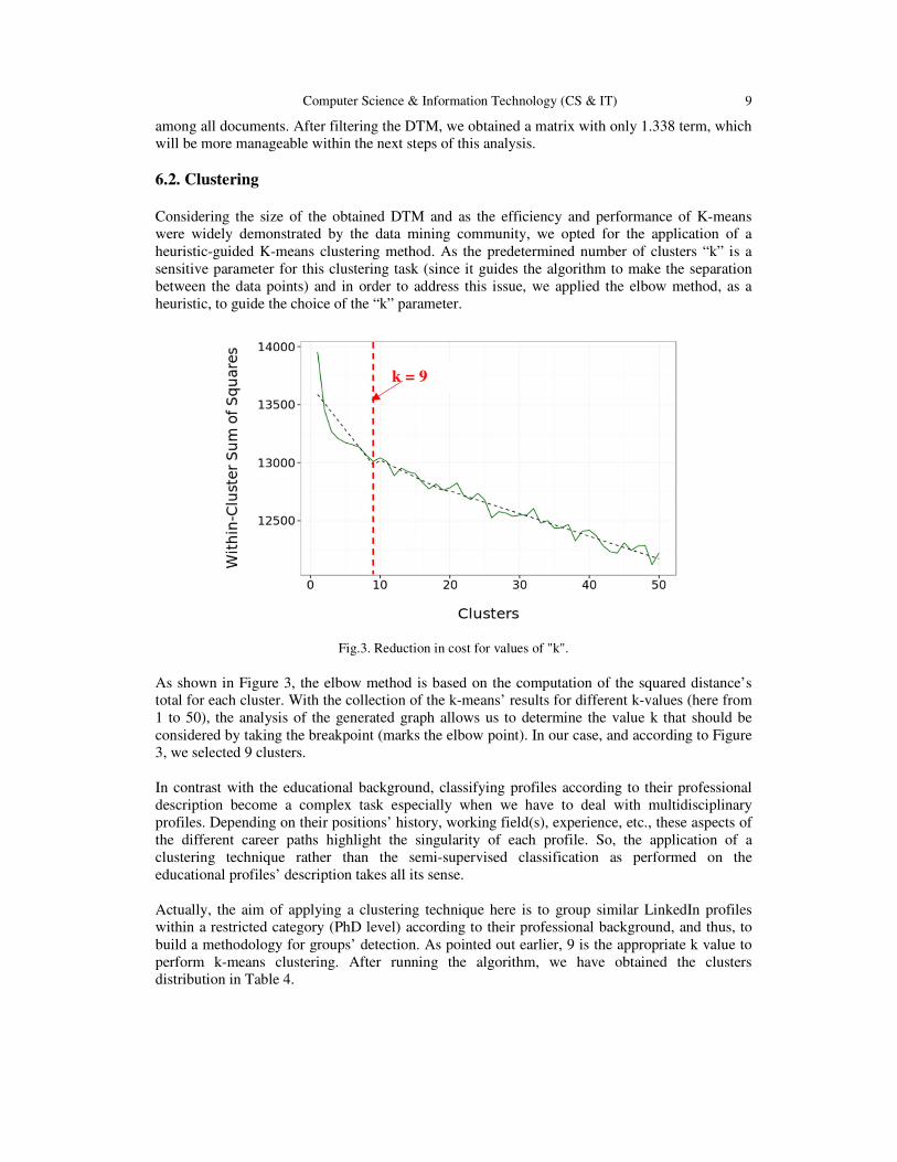
Considering the size of the obtained DTM and as the efficiency and performance of K-means were widely demonstrated by the data mining community, we opted for the application of a heuristic-guided K-means clustering method. As the predetermined number of clusters “k” is a sensitive parameter for this clustering task (since it guides the algorithm to make the separation between the data points) and in order to address this issue, we applied the elbow method, as a heuristic, to guide the choice of the “k” parameter.
Fig.3. Reduction in cost for values of "k".
As shown in Figure 3, the elbow method is based on the computation of the squared distance’s total for each cluster. With the collection of the k-means’ results for different k-values (here from 1 to 50), the analysis of the generated graph allows us to determine the value k that should be considered by taking the breakpoint (marks the elbow point). In our case, and according to Figure 3, we selected 9 clusters. In contrast with the educational background, classifying profiles according to their professional description become a complex task especially when we have to deal with multidisciplinary profiles. Depending on their positions’ history, working field(s), experience, etc., these aspects of the different career paths highlight the singularity of each profile. So, the application of a clustering technique rather than the semi-supervised classification as performed on the educational profiles’ description takes all its sense. Actually, the aim of applying a clustering technique here is to group similar LinkedIn profiles within a restricted category (PhD level) according to their professional background, and thus, to build a methodology for groups’ detection. As pointed out earlier, 9 is the appropriate k value to perform k-means clustering. After running the algorithm, we have obtained the clusters distribution in Table 4.
k = 9

10 Computer Science & Information Technology (CS & IT)
Table I. Number of profiles for each cluster.
Cluster id Number of profiles
1 199 2 2416 3 210 4 1846 5 374 6 5152 7 981 8 3090 9 75
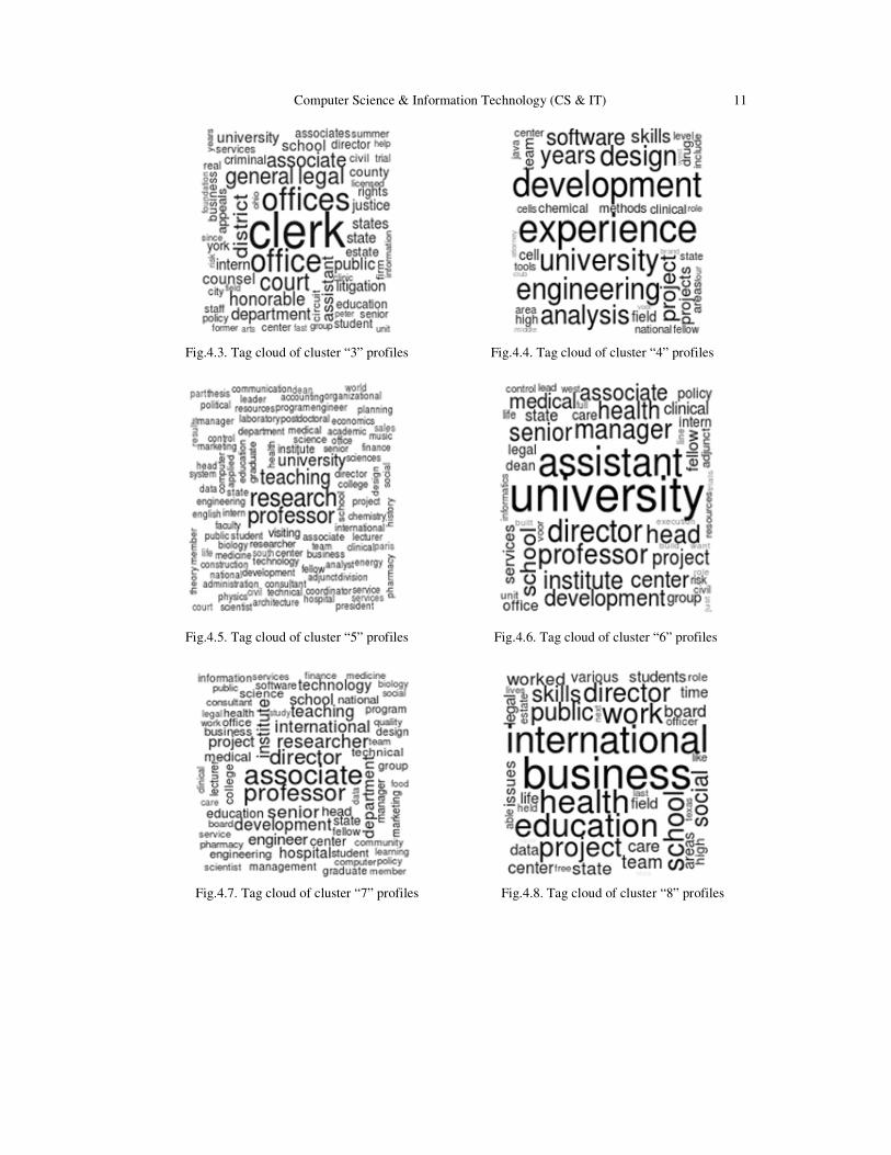
Furthermore, we have decided to analyse the most frequent terms in the professional description of each cluster’s profiles. We began by considering only terms associated to profiles belonging to each cluster. Then, we have sorted these terms according to their occurrence’s frequency among all profiles. And finally, we have constructed a Tag Cloud for each cluster in order to enable the visualization of these results. Consequently, we have obtained the 9 tag clouds. The existence of terms co-occurring among different tag clouds can be explained by the fact that there are some common terms used by the majority of profiles of this educational category (PhD level). So, encountering redundant terms such as “university”, “professor”, “teaching” etc., makes sense when considering this aspect. Indeed, scrutinizing each tag cloud can lead us to the characterization of the profiles’ groups. This exercise must be performed regarding all the professional aspects of a profile description (such as the “job position(s)” and “working field(s)”, etc.) but also by comparing each tag cloud to all others in order to spotlight its singularity.
Fig.4.1. Tag Cloud of cluster “1” profiles. Fig.4.2. Tag cloud of cluster “2” profiles.
Computer Science & Information Technology (CS & IT) 11
Fig.4.3. Tag cloud of cluster “3” profiles Fig.4.4. Tag cloud of cluster “4” profiles
Fig.4.5. Tag cloud of cluster “5” profiles Fig.4.6. Tag cloud of cluster “6” profiles
Fig.4.7. Tag cloud of cluster “7” profiles Fig.4.8. Tag cloud of cluster “8” profiles

12 Computer Science & Information Technology (CS & IT)
Fig.4.9. Tag cloud of cluster “9” profiles
Fig.4. Reduction in cost for values of "k".
7. RESULTS The characterization of the obtained clusters by interpreting their correspondent tag clouds can lead us to draw some conclusions about the different professional groups inside the PhD level category. A scrutiny of the tag clouds lead us to distinguish between these different groups. Administrative, technical, academic or business are the main discriminative aspects depicted here to characterize these profiles. Also, other major cross-cutting aspects must be considered as the working environment (private or public sector), field (health, technology, etc.) but also the position’s level (senior, director, assistant, etc.). The characterization process takes into account the most relevant terms used in all the profiles (professional description) constituting each cluster. An eventual subtraction of common tags could be conducted but a general interpretation of the tag clouds’ results should firstly takes into account the most frequent terms. Having 199 profiles, cluster number 1 (whose tag cloud is depicted in Fig 4.1) encompasses with the administrative public sector terminology (such as “public”, “county”, “district, etc.). The profiles of this group are related to the field of legal or juridical science. The second tag cloud describes high level academic researchers by the use of terms such as “university”, “professor”, “senior”, etc. In contrast with the first one which is also dealing with administrative profiles in the field of legal sciences, the third tag cloud describes professional profiles working in the private sector (“clerk”). The fourth tag cloud describes more technical profiles’, characterized via terms such as “development”, “engineering”, “design”, etc. Represented by its associated tag cloud, cluster 5 clearly spotlight academic profiles which are more involved in teaching experiences (“university”, “teaching”, “professor”, etc.) This aspect is consolidated by the existence of a terminology related to numerous fields of study (economics, technology, medical, etc.). The sixth cluster represents the most common profiles of the PhD level category (by grouping 5.152 profiles). It is characterized by academic profiles of the range of “assistant professor”, “project manager” and they are more research oriented.

Computer Science & Information Technology (CS & IT) 13
Tag cloud number 7 illustrates another group of profiles working in the academic field and mainly composed of “associate professor”, which are involved in international projects and may have some administrative responsibilities in their research organizations. The jargon used in the eighth tag cloud clearly describes business profiles working in international settings. Finally, and compared to the previous tag clouds, the last one describes a multidisciplinary profile which takes advantage of all the discussed aspects. With its 75 profiles, the ninth cluster is composed by LinkedIn profiles that encompass different job positions in management, research, teaching, etc.
8. DISCUSSION AND FUTURE WORK Very popular social networks, like Twitter or Facebook, have been intensively studied in the last years and it is reasonable easy to find available datasets. However, since LinkedIn is not as popular, there are not datasets gathering information (profiles and interactions) of this social network. In this paper, we have applied different social mining techniques to obtain our own dataset from LinkedIn which has been used as data source for our study. We consider that our dataset (composed of 5.7 million profiles) is representative of the LinkedIn activity for our study. Few proposals face analysis using this professional social network. In [29] the authors provide a statistical analysis of the professional background of LinkedIn profiles according to the job positions. Our approach also tackles profiles characterization, but focused on both the academic background and the professional background. Besides, our approach uses a really higher number of profiles instead of the 175 used in [29]. Clustering techniques were also applied in [30] with the aim of detecting groups or communities in this social network. They have also used as dataset a small group of 300 profiles. Finally, in [31] authors focus on detecting spammer’s profiles. Their work on 750 profiles concludes a third of the profiles were identified as spammers. For this study, we have collected more than 5.7 million LinkedIn profiles by scraping its public members’ directory. Then, and after cleaning the obtained data set, we have classified the profiles according to their educational background into 5 categories (PhD, master, bachelor, secondary, and others) and by considering the 4 levels of the UNESCO educational classification. NLP techniques were applied for this task but also for clustering the professional background of the profiles belonging to the PhD category. In this context, we have applied the well-known K-means algorithm conjunctly with the elbow method as a heuristic to determine the appropriate k-value. Finally, and for each cluster, we have generated the tag cloud associated to the professional description of the profiles. This characterization enables us to provide more insights about the professional groups of an educational category. Finally, and having established the former groups of educationally/professionally similar groups, we are currently working on given answers to the following questions: to what extent does educational background impact in the professional success? In how much time does this impact get its maximum level? Besides, and with the availability of temporal information in our data set (dates related to the job experience but also to the periods of studies or degrees), the application of predictive techniques is one of our highest priorities in order to provide career path recommendations according to the job market needs.
ACKNOWLEDGMENTS This work is funded by Spanish Ministry of Economy and Competitiveness under the National Science Program (TIN2010-20797 & TEC2013-47665-C4-3-R); the European Regional Development Fund (ERDF) and the Galician Regional Government under agreement for funding the Atlantic Research Center for Information and Communication Technologies (AtlantTIC); and the Spanish Government and the European Regional Development Fund (ERDF) under project TACTICA. This work is also partially funded by the European Commission under the Erasmus

14 Computer Science & Information Technology (CS & IT)
Mundus GreenIT project (3772227-1-2012-ES-ERA MUNDUS-EMA21). The authors also thank GRADIANT for its computing support.
REFERENCES [1] A. Mislove & M. Marcon & K. P. Gummadi & P. Druschel & B. Bhattacharjee (2007) “Measurement
and analysis of online social networks”, In: Proc. 7th ACM SIGCOMM Conf. Internet Meas. (IMC ’07), pp. 29-42, California.
[2] Y.-Y. Ahn & S. Han & H. Kwak & S. Moon & H. Jeong (2007) “Analysis of topological characteristics of huge online social networking services”, In: Proc. 16th Int. Conf. World Wide Web (WWW ’07), pp. 835-844, Alberta.
[3] S. Noraini & M. Tobi (2013) “The Use of Online Social Networking and Quality of Life”, In: Int. Conf. on Technology, Informatics, Management, Engineering & Environment, pp. 131–135, Malaysia.
[4] N. Deep “The Next Three Billion. In: LinkedIn Official Blog”, http://blog.linkedin.com/2014/04/18/the-next-three-billion/.
[5] J. Van Dijck (2013) “You have one identity: performing the self on Facebook and LinkedIn”, In: European Journal of Information Systems Media, Culture & Society, 35(2), pp. 199-215.
[6] V. Krishnamoorthy & B. Appasamy & C. Scaf (2013) “Using Intelligent Tutors to Teach Students How APIs Are Used for Software Engineering in Practice”, In: IEEE Transactions on Education, vol. 56, No. 3, pp. 355–363, Santa Barbara.
[7] A. Arasu & J. Cho & H. Garcia-molina (2011) “Searching the Web”, In: ACM Trans. Internet Technol., vol. 1, No. 1, pp. 2–43, New York.
[8] Y. Liu & A. Agah (2013) “Topical crawling on the web through local site-searches”, In: J. Web Eng., vol. 12, No. 3, pp. 203–214.
[9] J. Wang & Y. Guo (2012) “Scrapy-Based Crawling and User-Behavior Characteristics Analysis on Taobao”, In: IEEE Computer Society (CyberC), pp. 44-52, Sanya.
[10] L. Lovász: “Random Walks on Graphs : A Survey”, In: Combinatorics, Vol. 2, pp. 1-46. [11] M. Kurant & A. Markopoulou & P. Thira (2010) “On the bias of BFS (Breadth First Search)”, In:
22nd Int. Teletraffic Congr. (lTC 22), pp. 1–8. [12] M. Gjoka & M. Kurant & C. T. Butts & A. Markopoulou (2010) “Walking in Facebook : A Case
Study of Unbiased Sampling of OSNs”, In: IEEE Proceedings INFOCOM, San Diego. [13] C. Doerr & N. Blenn (2013) “Metric convergence in social network sampling”, In: Proc. 5th ACM
Work. HotPlanet (HotPlanet ’13), pp. 45-50, Hong Kong. [14] F. Buccafurri & G. Lax & A. Nocera & D. Ursin (2014) “Moving from social networks to social
internetworking scenarios: The crawling perspective”, In: Inf. Sci., Vol. 256, pp. 126–137, New York. [15] P. M. Nadkarni & L. Ohno-Machado & W. W. Chapman (2011) “Natural language processing: an
introduction”, In: J Am Med Inform Assoc, Vol. 18, 5, pp. 544-551. [16] E. Cambria & B. White (2014) “Jumping NLP curves: a review of natural language processing
research”, In: IEEE Computational Intelligence Magazine, Vol. 9, No. 2, pp. 48–57. [17] T. Brants (2004) “Natural Language Processing in Information Retrieval”, In: Proceedings of the 14th
Meeting of Computational Linguistics, pp. 1-13, Netherlands. [18] C. D. Manning & P. Raghavan & H. Schütze (2009) “An Introduction to Information Retrieval”, In:
Cambridge University Press. [19] A. N. K. Zaman & P. Matsakis , C. Brown (2011) “Evaluation of Stop Word Lists in Text Retrieval
Using Latent Semantic Indexing”, In: Sixth International Conference on Digital Information Management (ICDIM), pp. 133-136, Melbourne.
[20] W. B. Frakes & R. Baeza (1992) “Information Retrieval, Data Structures and Algorithms”, In: Prentice Hall, Inc, New Jersey.
[21] F. Shuweihdi (2009) “Clustering and Classification with Shape Examples”. In: Doctoral Thesis, University of Leeds.
[22] A. K. Jain & M. N. Murty & P. J. Flynn (1999) “Data clustering: a review”. In ACM Comput. Surv. 31, 3, pp. 264-323.
[23] J. MacQueen (1967) “Some Methods fir Classification and Analysis of Multivariate Observations”, In: Proc. of the fifth Berkeley Symposium on Mathematical Statistics and Probability (University of California Press), Vol.1, pp. 281-297, California.
Computer Science & Information Technology (CS & IT) 15
[24] P. Lingras & X. Huang (1967) “Statistical, Evolutionary, and Neurocomputing Clustering Techniques: Cluster-Based vs Object-Based Approaches”, In: Artif. Intell. Rev., Vol. 23, pp. 3-29.
[25] R. Tibshirani & W. Guenther & T. Hastie (2001) “Estimating the Number of Clusters in a Data Set via the Gap Statistic”, In: Journal of the Royal Statistical Society Series B.
[26] R. Thorndike (1953): “Who belongs in the family?”, In: Psychometrika, Vol.18, Nº4, pp. 267-276. [27] R.E. Bellman (1961): “Adaptive Control Processes”, In: Princeton University Press, Princeton, New
Jerse. [28] H. C. Wu & R. W. P. Luk & K. F. Wong & K. L. Kwok (2008) “Interpreting tf-idf term weights as
making relevance decisions”, In: ACM Transactions on Information Systems (TOIS), 26(3), pp. 1-37. [29] T. Case & A. Gardiner & P. Rutner & J. Dyer (2013) “A linkedin analysis of career paths of
information systems alumni”, In: Journal of the Southern Association for Information Systems, 1. [30] E. Ahmed & B. Nabli & A.,F. Gargouri (2014) “Group extraction from professional social network
using a new semi-supervised hierarchical clustering”, In: Knowl Inf Syst Vol. 40, 29–47. [31] V. M. Prieto & M. Álvarez & F. Cacheda (2013) “Detecting Linkedin Spammers and its Spam Nets”,
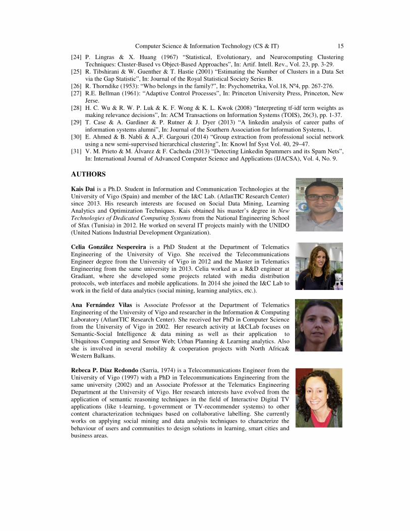
In: International Journal of Advanced Computer Science and Applications (IJACSA), Vol. 4, No. 9. AUTHORS Kais Dai is a Ph.D. Student in Information and Communication Technologies at the University of Vigo (Spain) and member of the I&C Lab. (AtlanTIC Research Center) since 2013. His research interests are focused on Social Data Mining, Learning Analytics and Optimization Techniques. Kais obtained his master’s degree in New
Technologies of Dedicated Computing Systems from the National Engineering School of Sfax (Tunisia) in 2012. He worked on several IT projects mainly with the UNIDO (United Nations Industrial Development Organization). Celia González Nespereira is a PhD Student at the Department of Telematics Engineering of the University of Vigo. She received the Telecommunications Engineer degree from the University of Vigo in 2012 and the Master in Telematics Engineering from the same university in 2013. Celia worked as a R&D engineer at Gradiant, where she developed some projects related with media distribution protocols, web interfaces and mobile applications. In 2014 she joined the I&C Lab to work in the field of data analytics (social mining, learning analytics, etc.). Ana Fernández Vilas is Associate Professor at the Department of Telematics Engineering of the University of Vigo and researcher in the Information & Computing Laboratory (AtlantTIC Research Center). She received her PhD in Computer Science from the University of Vigo in 2002. Her research activity at I&CLab focuses on Semantic-Social Intelligence & data mining as well as their application to Ubiquitous Computing and Sensor Web; Urban Planning & Learning analytics. Also she is involved in several mobility & cooperation projects with North Africa& Western Balkans. Rebeca P. Díaz Redondo (Sarria, 1974) is a Telecommunications Engineer from the University of Vigo (1997) with a PhD in Telecommunications Engineering from the same university (2002) and an Associate Professor at the Telematics Engineering Department at the University of Vigo. Her research interests have evolved from the application of semantic reasoning techniques in the field of Interactive Digital TV applications (like t-learning, t-government or TV-recommender systems) to other content characterization techniques based on collaborative labelling. She currently works on applying social mining and data analysis techniques to characterize the behaviour of users and communities to design solutions in learning, smart cities and business areas.

16 Computer Science & Information Technology (CS & IT)
INTENTIONAL BLANK
David C. Wyld et al. (Eds) : ITCS, CST, JSE, SIP, ARIA, DMS - 2015
pp. 17–24, 2015. © CS & IT-CSCP 2015 DOI : 10.5121/csit.2015.50102
UNDERSTANDING PHYSICIANS’
ADOPTION OF HEALTH CLOUDS
Tatiana Ermakova
Department of Information and Communication Management,
Technical University of Berlin, Berlin [email protected]
ABSTRACT
Recently proposed health applications are able to enforce essential advancements in the
healthcare sector. The design of these innovative solutions is often enabled through the cloud
computing model. With regards to this technology, high concerns about information security
and privacy are common in practice. These concerns with respect to sensitive medical
information could be a hurdle to successful adoption and consumption of cloud-based health
services, despite high expectations and interest in these services. This research attempts to
understand behavioural intentions of healthcare professionals to adopt health clouds in their
clinical practice. Based on different established theories on IT adoption and further related
theoretical insights, we develop a research model and a corresponding instrument to test the
proposed research model using the partial least squares (PLS) approach. We suppose that
healthcare professionals’ adoption intentions with regards to health clouds will be formed by
their outweighing two conflicting beliefs which are performance expectancy and medical
information security and privacy concerns associated with the usage of health clouds. We
further suppose that security and privacy concerns can be explained through perceived risks.
KEYWORDS
Cloud Computing, Healthcare, Adoption, Physician, Security and Privacy Concerns
1. INTRODUCTION
Nowadays, healthcare and medical service delivery are on the way to be revolutionized
([7][7],[21]). Due to the recently proposed solutions, medical data can be easily shared and
collaboratively used by healthcare professionals involved in the medical treatment [42][42], while
novice surgeons can automatically be assisted in their surgical procedures [32][32] and physicians
can be supported to make their therapy-related decisions [30][30]. The design of these apparently
important innovative healthcare solutions is often enabled through the cloud computing model,
which is known for providing adequate computing and storage resources on demand [33][33].
However, the immediate involvement of the cloud computing’s third-party as well as
communication via the open Internet landscape might lead to unexpected risks (e.g., legal
problems) ([6][6],[35]) and therefore cause intense concerns among medical workers with respect
to cloud computing companies’ ability and willingness to protect disclosed medical information
([24], [36], [43]). While online medical service providers currently show interest in collecting
medical information of their customers ([22][22],[25]), through the misuse of medical
information the service users might get subject to harassment by marketers of medical products
and services, and discrimination by employers, healthcare insurance agencies, and associates

18 Computer Science & Information Technology (CS & IT)
([3][3],[27]). The exposure of security and privacy concerns related to sensitive medical
information could be a serious hurdle to successful adoption and consumption of cloud-based
health services, as repeatedly demonstrated by prior empirical evidence in other healthcare
settings ([1][1], [2], [3], [18], [15], [29], [6], [35], and [5]).
This research examines which determinants can explain the extent to which medical workers will
be willing to adopt health clouds in their daily work. To conduct the research, we follow the
guidelines proposed by [44][44], [38], [31] and [19]. We build on well-established theories and
works on adoption of information technologies ([47], [48]) and existing theoretical insights into
the factors influencing healthcare IT and cloud computing adoption. We further draw on utility
maximization theory ([3], [12]) arguing that one tries to maximize his or her total utility. We
suppose the utility function to be given by the trade-off between expected positive and negative
outcomes in a healthcare professional’s decision-making process with regards to the usage of
health clouds.
The paper is divided into four sections. In Section 2, we introduce the background of our
research, highlight main theoretical foundations and formulate research hypothesis. Section 3
proceeds with presenting the research model where we illustrate the hypothesized relations. It
further deals with the instrument developed to test the proposed research model using the partial
least squares (PLS) approach ([19][19], [20], [44]). We conclude by recapitulating the results of
this work, extensively discussing its limitations and thus giving recommendations for further
research.
2. BACKGROUND AND THEORETICAL FOUNDATIONS
The availability of medical data is of utmost importance to physicians during the medical service
delivery [42][42]. The healthcare sector can further profit from modern data analysis techniques.
Their application fields in the healthcare area range from disease detection, disease outbreak
prediction, and choice of a therapy to useful information extraction from doctors’ free-note
clinical notes, and medical data gathering and organizing [21]. These techniques can also be
applied to assessment of plausibility and performance of medical services and medical therapies
development [7]. Recently, [32] introduced an interactive three-dimensional e-learning portal for
novice surgeons. Under real time conditions, their surgical procedures are to be compared to the
practice of experienced surgeons. [30] presented a decision support system aimed to assist
physicians in finding a successful treatment for some certain illness based on the currently
available best practices and the characteristics of a given patient.
By provisioning adequate capacities to store and process huge amounts of data, cloud computing
facilitates the design of these innovative applications in the healthcare area. However, this
technology is also known for users’ concerns about their information security and privacy ([24],
[36]). While the providers of healthcare-related websites are interested in collecting medical
information ([22][22], [25]), the misuse of medical information might result in different
harassment and discrimination scenarios for patients ([3],[27]). In the recent past, there were
cases where, based on disclosed medical information, marketers of medical products and services
sent their promotional offers; employers refused to hire applicants and even fired employees;
insurance firms denied life insurances. The exposure of the concerns surrounding information
security and privacy could therefore negatively affect adoption and consumption of cloud-based
health services, as multiple empirical studies demonstrated this in the healthcare context ([1], [2],
[3][3], [18], [15], [29], [6], [35] and [5]) and other settings ([13], [14] and [40]).
In the present work, we try to understand the predictors of behavioural intention of healthcare
professionals to adopt health clouds in their work. In the research related to management of

Computer Science & Information Technology (CS & IT) 19
information systems (MIS), a variety of theories have been applied to explain an individual’s
adoption of information technologies. Among others, these include theories of reasoned action
(TRA), planned behaviour (TPB), technology acceptance model (TAM), and unified theory of
acceptance and use of technology (UTAUT) ([47], [48]). In line with these theories, we suppose
that healthcare professionals’ adoption of health clouds is a product of beliefs surrounding the
system. We additionally assume that medical workers’ intentions are consistent with utility
maximization theory ([3], [12]) which posits that an individual attempts to maximize his or her
total utility. As usage of health clouds is associated with numerous risks for a healthcare
professional, we suppose that his or her utility function in the presented context is given by the
calculus of conflicting beliefs which involve performance expectancy of the services, on one side,
and associated security and privacy concerns about medical information, on the other side. We
further postulate that information security and privacy concerns result from perceived risks.
2.1 Performance Expectancy
In one of the recent works on information technology acceptance, Venkatesh et al. [47] defines
performance expectancy as the extent to which individuals believe that using the information
technology is helpful in attaining certain gains in their job performance. Performance expectancy
and other factors that pertain to performance expectancy such as perceived usefulness are
generally shown to be the strongest predictors of behavioural intention [47]. Previous work
suggests that healthcare professionals tend to be higher willing to adopt technological advances in
their practice the higher they perceive their usefulness ([17], [8], [46], [35]). Similarly, cloud
computing is more likely to be adopted the more beneficial it appears to the decision maker ([23],
[28], [29], [36]). Therefore, we hypothesize that:
Hypothesis 1. Performance expectancy will be positively associated with behavioural intention to
accept health clouds.
2.2 Security and Privacy Concerns
Online companies rely on use of their customers’ personal information to select their marketing
strategies ([36], [25]). As a result of this, Internet users view their privacy as being invaded. A
recent survey revealed that 90% of Americans and Britons felt concerned about their online
privacy and over 70% of Americans and 60% of Britons were even higher concerned than in the
previous year [43].
Healthcare professionals appear to be ones of the most anxious Internet users in terms of
information privacy. Dinev and Hart [13] argue that Internet “users with high social awareness
and low Internet literacy tend to be the ones with the highest privacy concerns”. Although this
group of users constitute the intellectual core of society, they are not able or willing to keep up
with protecting technologies while using the Internet. Simon et al. [39] further state that
physicians are worried about patient privacy even more than the patients themselves.
In this study, privacy concerns are related to healthcare professionals’ beliefs regarding cloud
computing companies’ ability and willingness to protect medical information ([40], [4], [36]).
The dimensions of privacy concerns involve errors, improper access, collection, and unauthorized
secondary usage.
Due to the open Internet infrastructure vulnerable to multiple security threats [36], we further
consider security concerns. They refer to healthcare professionals’ beliefs regarding cloud
computing companies’ ability and willingness to safeguard medical information from security
breaches ([4], [36]). The dimensions of security concerns include information confidentiality and

20 Computer Science & Information Technology (CS & IT)
integrity, authentication (verification) of the parties involved and non-repudiation of transactions
completed.
Similarly to [4], we distinguish six dimensions of the combined security and privacy concerns,
where we consider the dimensions of errors and improper access to be equivalent to the
expectancy are to be measured with items adapted from Venkatesh et al. ([47], [48]). Security and
privacy concerns are to be explored at a more detailed level, as recommended by [1]. With
regards to the concerns, we draw on the multi-dimensional view proposed by Bansal [4]. The
dimensions of privacy-related concerns, i.e., collection, errors, unauthorized secondary use, and
improper access, originate from the work by Smith et al. [40] and were validated in healthcare
privacy studies ([15], [18]). To measure the factors associated with collection, integrity/errors,
and confidentiality/improper access, the questions from [18] were adapted. For the secondary use
construct, we took items from [12]. Measures for the remaining underlying factors, i.e.,
authentication and non-repudiation, were developed based on [4]. To measure perceived risks, we
rely on the items by [16].
Table 1. Research Model Constructs and Related Questionnaire Items
Construct Items
Behavioural Intention to
Adopt Health Clouds
(based on [47], [48])
Given I get the system offered in the future and the patient consent for
medical information transmission over the system is given, …
… I intend to use it whenever possible.
… I plan to use it to the extent possible.
… I expect that I have to use it.
Performance Expectancy
(based on [47], [48])
Using the system would make it easier to do my job.
I would find the system useful in my job.
If I use the system, I will spend less time on routine job tasks.
Security and Privacy
Concerns – Integrity / Errors
(based on [4], [40], [18])
I would be concerned that in the system…
… medical information can be modified (altered, corrupted).
… medical information is not enough protected against modifications.
… accurate medical information can hardly be guaranteed.
Security and Privacy
Concerns – Confidentiality /
Improper Access
(based on [4], [40], [18])
I would be concerned that in the system…
… medical information can be accessed by unauthorized people.
… medical information is not enough protected against unauthorized
access.
… authorized access to medical information can hardly be guaranteed.
Security and Privacy
Concerns – Authentication
(based on [4])
I would be concerned that in the system…
… transactions with a wrong user can take place in the system.
… verifying the truth of a user in the system is not enough ensured.
… transacting with the right user in the system can hardly be
guaranteed.
Security and Privacy
Concerns – Nonrepudiation
(based on [4])
I would be concerned that transactions in the system …
…. could be declared untrue.
… are disputable.
… are deniable.
Security and Privacy
Concerns – Collection
(based on [4], [40], [18])
I would be concerned that medical information transmitted over the
system …
… does not get deleted from the cloud.
… is kept as a copy.
… is collected by the cloud provider.
Security and Privacy
Concerns – Unauthorized
Secondary Use
(based on [4], [40], [12])
I would be concerned that medical information transmitted over the
system can be …
… used in a way I did not foresee.
… misused by someone unintended.
… made available/sold to companies or unknown parties without your
knowledge.

Computer Science & Information Technology (CS & IT) 21
Perceived Risks
(based on [16])
In general, it would be risky to transmit medical information over the
system.
Transmitting medical information over the system would involve many
unexpected problems.
I would not have a good feeling when transmitting medical information
over the system.
The respondents are supposed to be presented one of the above mentioned scenarios. They further
will be asked to provide their answers to the questions on a 7 Likert scale (e.g., 1: Not likely at
all, 2: Highly unlikely, 3: Rather unlikely, 4: Neither likely nor unlikely, 5: Rather likely, 6:
Highly likely, 7: Fully likely). Additionally, they will be asked about practice period [9], their
workplace location (e.g. rural or urban) ([35], [9]), gender, and age, etc. [35]. These questions
will mainly allow describing the sample.
3. CONCLUSION, LIMITATIONS AND SUGGESTIONS FOR FUTURE
RESEARCH
In this work, we defined a theoretical model aimed to explain behavioural intention of healthcare
professionals to adopt health clouds in their clinical practice. We operationalized the research
model and transferred it into a structural equation model to further analyse with the PLS
approach.
Drawing on utility maximization theory and further related research, we suppose that healthcare
professionals’ adoption intentions with regards to health clouds will be formed by outweighing
two conflicting beliefs. They involve expected performance expectancy and security and privacy
concerns associated with the usage of health clouds. We further postulate that security and
privacy concerns can be explained through perceived risks.
Our work implies some limitations. First, there might be some other possible casual relationships
between the constructs proposed in the research model. For example, [46] hypothesize that EMR
security/confidentiality influences its perceived usefulness, while [17] find a positive relationship
between perceived importance of data security and perceived usefulness of electronic health
services. As identified by [26], perceived privacy risk directly influences personal information
disclosure in the context of online social networks. In our future research, we are going to verify
all possible paths, as recommended by [20].
Second, we left some other factors out of consideration such as effort expectancy, social
influence, and facilitating conditions which are often investigated and can extend the study in the
future.
Venkatesh et al. [47] define effort expectancy as referring to the extent to which an individual
finds the system easy to use. The factor is also captured by perceived ease of use specified in
TAM. Perceived ease of use is important for potential cloud computing users ([28], [36]).
Physicians view easy-to-use services as more useful and stronger intend to use them ([17], [6],
[35], [6]). Contrary to these findings and other previous research assertions (e.g., [47], [48]),
perceived ease of use did not exert any significant effects on perceived usefulness or attitude,
when tested in the telemedicine context [8]. The authors suggest that physicians comprehend new
information technologies more easily and quickly than other user groups do. Alternatively, the
importance of perceived ease of use may be weakened by increases in general competence or staff
assistance [8]. These aspects are implied in the concept of facilitating conditions which relates to
the extent to which individuals believe in the existence of an organizational and technical

22 Computer Science & Information Technology (CS & IT)
infrastructure to support their system use [47]. They were found to play a role in formation of
behavioural intention to use cloud computing in hospital [29] and perceived usefulness of
healthcare information technologies ([8], [34], [6], [35]).
Social influence refers to the degree to which individuals perceive that others’ beliefs about their
system use are important [47]. Being differently labelled across studies, social influence was
found to have contradictory results when tested with regards to behavioural intention. Cloud
computing users were significantly guided by the way they believe they are viewed by others as
having used the cloud computing technology [28]. However, practicing physicians’ intentions to
use telemedicine technology were not significantly influenced by social norms [8]. Dinev and Hu
[11] observe subjective norm influencing behavioural intention rather for IT aware groups. Dinev
and Hu believe that the more IT knowledgeable the group are, the more they communicate about
IT related issues and are willing to learn IT solutions their peers already use.
Finally, some variables which are to be used to describe the sample (e.g., workplace location) can
further be controlled for their role. As observed by [35], urban hospitals could be expected to
adopt innovative solutions rather than rural ones. Hospitals located outside cities and towns are
the only alternative for people living nearby. So they do not have to compete with others in
adopting new technologies. Furthermore, they are typically under-occupied and have little
financial support.
ACKNOWLEDGEMENTS
The work presented in this paper was performed in the context of the TRESOR research project
[42]. TRESOR is funded by the German Federal Ministry of Economic Affairs and Energy
(BMWi).
REFERENCES
[1] Angst, C.M. & Agarwal, R. (2009) “Adoption of Electronic Health Records in the Presence of
Privacy Concerns: The Elaboration Likelihood Model and Individual Persuasion”, MIS Quarterly,
Vol. 33, No. 2, pp. 339-370.
[2] Bansal, G., Zahedi, F. & Gefen, D. (2007) “The Impact of Personal Dispositions on Privacy and Trust
in Disclosing Health Information Online”, Americas Conference on Information Systems.
[3] Bansal, G., Zahedi, F. & Gefen, D. (2010) “The Impact of Personal Dispositions on Information
Sensitivity, Privacy Concern and Trust in Disclosing Health Information Online”, Decision Support
Systems, Vol. 49, No. 2, pp. 138-150.
[4] Bansal, G. (2011) “Understanding the Security in Privacy-Security Concerns: A Theoretical and
Empirical Examination”, Americas Conference on Information Systems.
[5] Bassi, J., Lau, F. & Lesperance, M. (2012) “Perceived Impact of Electronic Medical Records in
Physician Office Practices: A Review of Survey-Based Research”, Interactive Journal of Medical
Research, Vol. 1, No. 2, e3.
[6] Boonstra, A. & Broekhuis, M. (2010) “Barriers to the Acceptance of Electronic Medical Records by
Physicians from Systematic Review to Taxonomy and Interventions”, BMC Health Services
Research, Vol. 10, No. 231.
[7] BMWi (2014) “Anwendungen für den Gesundheitssektor”, http://www.trusted-cloud.de/239.php,
accessed November 6, 2014.
[8] Chau, P.Y.K. & Hu, P.J.-H. (2001)”Information Technology Acceptance by Individual Professionals:
A Model Comparison Approach”, Decision Sciences, Vol. 32, No. 4, pp. 699–719.
[9] DesRoches, C.M., Campbell, E.G., Rao, S.R., Donelan, K., Ferris, T.G., Jha, A., Kaushal, R, Levy,
D.E., Rosenbaum, S., Shields, A.E. & Blumenthal, D. (2008) “Electronic Health Records in
Ambulatory Care – A National Survey of Physicians”, The New England Journal of Medicine, Vol.
359, No. 1, pp. 50-60.

Computer Science & Information Technology (CS & IT) 23
[10] Dinev, T. & Hart, P. (2004) “Internet Privacy Concerns and their Antecedents - Measurement Validity
and a Regression Model”, Behaviour & Information Technology, Vol. 23, No. 6, pp. 413-422.
[11] Dinev, T. & Hu, Q. (2005) “The Centrality of Awareness in the Formation of User Behavioral
Intention Toward Preventive Technologies in the Context of Voluntary Use”, Conference for Special
Interest Group on Human-Computer Interaction.
[12] Dinev, T. & Hart, P. (2006) “An Extended Privacy Calculus Model for E-Commerce Transactions”,
Information Systems Research, Vol. 17, No. 1, pp. 61–80.
[13] Dinev, T. & Hart, P. (2006) “Internet Privacy Concerns and Social Awareness as Determinants of
Intention to Transact”, International Journal of E-Commerce, Vol. 10, No. 2, pp. 7-29.
[14] Dinev, T., Bellotto, M., Hart, P., Russo, V., Serra, I. & Colautti, C. (2006) “Internet Users' Privacy
Concerns and Beliefs about Government Surveillance: an Exploratory Study of Differences between
Italy and the United States”, Journal of Global Information Management, Vol. 14, No. 4, pp. 57–93.
[15] Dinev, T., Albano, V., Xu, H., D’Atri, A. & Hart, P. (2012) “Individual’s Attitudes Towards
Electronic Health Records – A Privacy Calculus Perspective”, Annals of Information Systems.
[16] Dinev, T., Xu, H., Smith, H.J. & Hart, P. (2013) “Information Privacy and Correlates: An Empirical
Attempt to Bridge and Distinguish Privacy-Related Concepts”, European Journal of Information
Systems, Vol. 22, No. 3, pp. 295-316.
[17] Dünnebeil, S., Sunyaev, A., Blohm, I., Leimeister, J.M. & Krcmar, H. (2012) “Determinants of
Physicians’ Technology Acceptance for e-Health in Ambulatory Care”, International Journal of
Medical Informatics, Vol. 81, No. 11, pp. 746-760.
[18] Ermakova, T., Fabian, B., & Zarnekow, R. (2014) “Acceptance of Health Clouds – a Privacy Calculus
Perspective”, European Conference on Information Systems.
[19] Gefen, D., Straub, D.W. & Boudreua, M.C. (2000) “Structural Equation Modeling and Regression:
Guidelines for Research Practice”, Communications of the Association for Information Systems, Vol.
4, No. 7, pp. 1-78.
[20] Gefen, D., Rigdon, E. & Straub, D. (2011) “An Update and Extension to SEM Guidelines for
Administrative and Social Science Research”, MIS Quarterly, Vol. 35, No. 2, pp. iii-xiv.
[21] Hardesty, L. (2013) “Big Medical Data”, http://web.mit.edu/newsoffice/2013/big-medical-data-
0125.html, accessed November 8, 2014.
[22] Huesch, M. D. (2013) “Privacy Threats when Seeking Online Health Information”, JAMA Internal
Medicine, Vol. 173, No. 19, pp. 1838-1840.
[23] Hsu, P.-F., Ray, S. & Li-Hsieh, Y.-Y. (2014) “Examining Cloud Computing Adoption Intention,
Pricing Mechanism, and Deployment Model”, International Journal of Information Management,
Vol. 34, No. 4, pp. 474–488.
[24] Ion, I., Sachdeva, N., Kumaraguru, P. & Capkun, S. (2011) “Home is Safer than the Cloud! Privacy
Concerns for Consumer Cloud Storage“, Symposium on Usable Privacy and Security.
[25] Kaletsch, A. & Sunyaev, A. (2011). “Privacy Engineering: Personal Health Records in Cloud
Computing Environments”. International Conference on Information Systems.
[26] Krasnova, H., Spiekermann, S., Koroleva, K. & Hildebrandt, T. (2009) “Online Social Networks:
Why We Disclose”, Journal of Information Technology, Vol. 25, No. 2, pp. 109–125.
[27] Laric, M.V., Pitta, D.A. & Katsanis, L.P. (2009) “Consumer Concerns for Healthcare Information
Privacy: A Comparison of U.S. and Canadian Perspectives”, Research in Healthcare Financial
Management, Vol. 12, No. 1, pp. 93-111.
[28] Li, Y. & Chang, K.-C. (2012) “A Study on User Acceptance of Cloud Computing: A Multi-
Theoretical Perspective”, Americas Conference on Information Systems.
[29] Lian, J., Yen, D.C. & Wang, Y. (2014) “An Exploratory Study to Understand the Critical Factors
Affecting the Decision to adopt Cloud Computing in Taiwan Hospital”, International Journal of
Information Management, Vol. 34, No. 1, pp. 28-36.
[30] Lupse, O. S., Stoicu-Tivadar, L. & Golie, C. (2013) “Assisted Prescription Based on Successful
Treatments”, E-Health and Bioengineering Conference.
[31] MacKenzie, S.B., Podsakoff, P.M. & Podsakoff, N.P. (2011) “Construct Measurement and Validation
Procedures in MIS and Behavioral Research: Integrating New and Existing Techniques”, MIS
Quarterly, Vol. 35, No. 2, pp. 293-334.
[32] Mani, G. & Li, W. (2013) “3D Web Based Surgical Training Through Comparative Analysis”,
International Conference on 3D Web.
[33] Mell, P. & Grance, T. (2012). “The NIST Definition of Cloud Computing”, National Institute of
Standards and Technology, http://csrc.nist.gov/publications/nistpubs/800-145/SP800-145.pdf,
accessed March 12, 2014.
24 Computer Science & Information Technology (CS & IT)
[34] Moores, T.T. (2012) “Towards an Integrated Model of IT Acceptance in Healthcare”, Decision
Support Systems, Vol. 53, No. 3, pp. 507-516.
[35] Najaftorkaman, M. & Ghapanchi, A.H. (2014) „Antecedents to the User Adoption of Electronic
Medical Record”, Pacific Asia Conference on Information Systems.
[36] Opitz, N., Langkau, T.F., Schmidt, N.H. & Kolbe, L.M. (2012) “Technology Acceptance of Cloud
Computing: Empirical Evidence from German IT Departments”, Hawaii International Conference on
System Sciences.
[37] Pavlou, P., Liang, H. & Xue, Y. (2007) “Understanding and Mitigating Uncertainty in Online
Exchange Relationships: A Principle–Agent Perspective?”, MIS Quarterly, Vol. 31, No. 1, pp. 105–
136.
[38] Petter, S., Straub, D. & Rai, A. (2007) “Specifying Formative Constructs in Information Systems
Research”, MIS Quarterly, Vol. 33, No. 4, pp. 623-656.
[39] Simon, S.R., Kalshal, R., Cleary, P.D., Jenter, C.A., Volk, L.A., Oray, E.J., Burdick E., Poon, E.G. &
Batees, W.W. (2007) “Physicians and Electronic Health Records: A Statewide Survey”, Archives of
Internal Medicine, Vol. 167, No. 5, pp. 507-512.
[40] Smith, H.J., Milberg, J.S. & Burke, J.S. (1996) “Information Privacy: Measuring Individuals’
Concerns about Organizational Practices”, MIS Quarterly, Vol. 20, No. 2, pp. 167-196.
[41] European Parliament and Council (1995) “Directive 95/46/EC of the European Parliament and of the
Council of 24 October 1995 on the Protection of Individuals with Regard to the Processing of
Personal Data and on the Free Movement of Such Data”, Official Journal, Vol. 281, No. 31, pp. 31 –
50.
[42] TRESOR (2014) “TRESOR”, http://www.cloud-tresor.com/, accessed November 6, 2014.
[43] TRUSTe (2014) “TRUSTe”, http://www.truste.com/, accessed August 19, 2014.
[44] Urbach, N. & Ahlemann, F. (2010) “Structural Equation Modeling in Information Systems Research
Using Partial Least Squares”, Journal of Information Technology Theory and Application, Vol. 11,
No. 2, pp. 5-40.
[45] U.S. Department of Health & Human Services (1996) “Health Insurance Portability and
Accountability Act of 1996 (HIPAA)”, http://www.hhs.gov/ocr/privacy/, accessed December 3, 2014.
[46] Vathanophas, V. & Pacharapha, T. (2010) “Information Technology Acceptance in Healthcare
Service: The Study of Electronic Medical Record (EMR) in Thailand”, Technology Management for
Global Economic Growth.
[47] Venkatesh, V., Morris, M. G., Davis, G. B. & Davis, F. D. (2003) “User Acceptance of Information
Technology: Toward a Unified View”, MIS Quarterly, Vol. 27, No. 3, pp. 425–478.
[48] Venkatesh, V., Thong, J.Y.L. & Xu, X. (2012) “Consumer Acceptance and Use of Information
Technology: Extending the Unified Theory of Acceptance and Use of Technology”, MIS Quarterly,
Vol. 36 No. 1, pp. 157-178.
[49] Xu, H., Dinev, T., Smith, H. J. & Hart, P. (2008) “Examining the Formation of Individual‘s Privacy
Concerns: Toward an Integrative View”, International Conference on Information Systems.
[50] Xu, H., Dinev, T., Smith, H. J. & Hart, P. (2011) “Information Privacy Concerns: Linking Individual
Perceptions with Institutional Privacy Assurances”, Journal of the Association for Information
Systems, Vol. 12, No. 12, pp. 798-824.
AUTHOR Tatiana Ermakova is a research assistant at the Department of Information and
Communication Management of the Technical University of Berlin. She holds a
bachelor degree in Economics and a diploma degree in Applied Informatics in
Economics from the Russian Academy of Economics, a M.Sc. in Information Systems
from Humboldt University of Berlin.

David C. Wyld et al. (Eds) : ITCS, CST, JSE, SIP, ARIA, DMS - 2015
pp. 25–31, 2015. © CS & IT-CSCP 2015 DOI : 10.5121/csit.2015.50103
IMAGE RETRIEVAL USING VLAD WITH
MULTIPLE FEATURES
Pin-Syuan Huang, Jing-Yi Tsai, Yu-Fang Wang, and Chun-Yi Tsai
Department of Computer Science and Information Engineering,
National Taitung University, Taiwan, R.O.C. {u10011104,u10011127,u10011139}@ms100.nttu.edu.tw;
ABSTRACT
The objective of this paper is to propose a combinatorial encoding method based on VLAD to
facilitate the promotion of accuracy for large scale image retrieval. Unlike using a single
feature in VLAD, the proposed method applies multiple heterogeneous types of features, such as
SIFT, SURF, DAISY, and HOG, to form an integrated encoding vector for an image
representation. The experimental results show that combining complementary types of features
and increasing codebook size yield high precision for retrieval.
KEYWORDS
VLAD, SIFT, SURF, DAISY, HOG
1. INTRODUCTION
Image retrieval is one of the classical problems in computer vision and machine intelligence. The
challenge of image retrieval is mainly aimed at trade-off between computing costs and the
precision of retrieval due to the large scale data, including the large size of a single image and the
large number of all images. In this paper, we propose an combinatorial encoding algorithm based
on VLAD[6,9] with multiple features to achieve the goal of large scale image retrieval. VLAD
cluster all features descriptors extracted from training images to find a certain number of
centroids. These centroids are treated as code words or visual words, and thus form a codebook.
Each image from either testing dataset or training dataset can be further encoded to a vector with
fixed dimension using the trained codebook. The VLAD encoding contributes a key concept that
it encodes any image by a collection of code words encoding vector with a consensus dimension.
The rest of this paper is organized as follows. Section 2 reviews the previous work VLAD
algorithm, section 3 elaborates the proposed method, section 4 shows experimental results, and a
conclusion is given in section 5.
2. RELATED WORK
2.1. VLAD Algorithm
VLAD(vector of locally aggregated descriptors) is proposed by Jegou[6] in 2010. Similar as
BOF(bag-of-features)[10], VLAD aims at representing one single image by a fixed number of
feature vectors aggregated by all feature descriptors extracted from this image. Such a
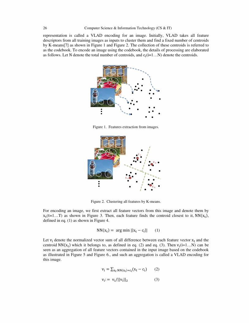
26 Computer Science & Information Technology (CS & IT)
representation is called a VLAD encoding for an image. Initially, VLAD takes all feature
descriptors from all training images as inputs to cluster them and find a fixed number of centroids
by K-means[7] as shown in Figure 1 and Figure 2. The collection of these centroids is referred to
as the codebook. To encode an image using the codebook, the details of processing are elaborated
as follows. Let N denote the total number of centroids, and c�(i=1…N) denote the centroids.
Figure 1. Features extraction from images.
Figure 2. Clustering all features by K-means.
For encoding an image, we first extract all feature vectors from this image and denote them by
x�(t=1…T) as shown in Figure 3. Then, each feature finds the centroid closest to it, NN�x�,
defined in eq. (1) as shown in Figure 4.
NN�x� = arg min ||x� − c�|| (1)
Let v� denote the normalized vector sum of all difference between each feature vector x� and the
centroid NN�x� which it belongs to, as defined in eq. (2) and eq. (3). Then v�(i=1…N) can be
seen as an aggregation of all feature vectors contained in the input image based on the codebook
as illustrated in Figure 5 and Figure 6., and such an aggregation is called a VLAD encoding for
this image.
v� = ∑ �x� − c���:�������� (2)
v�: = v�/||v�||� (3)
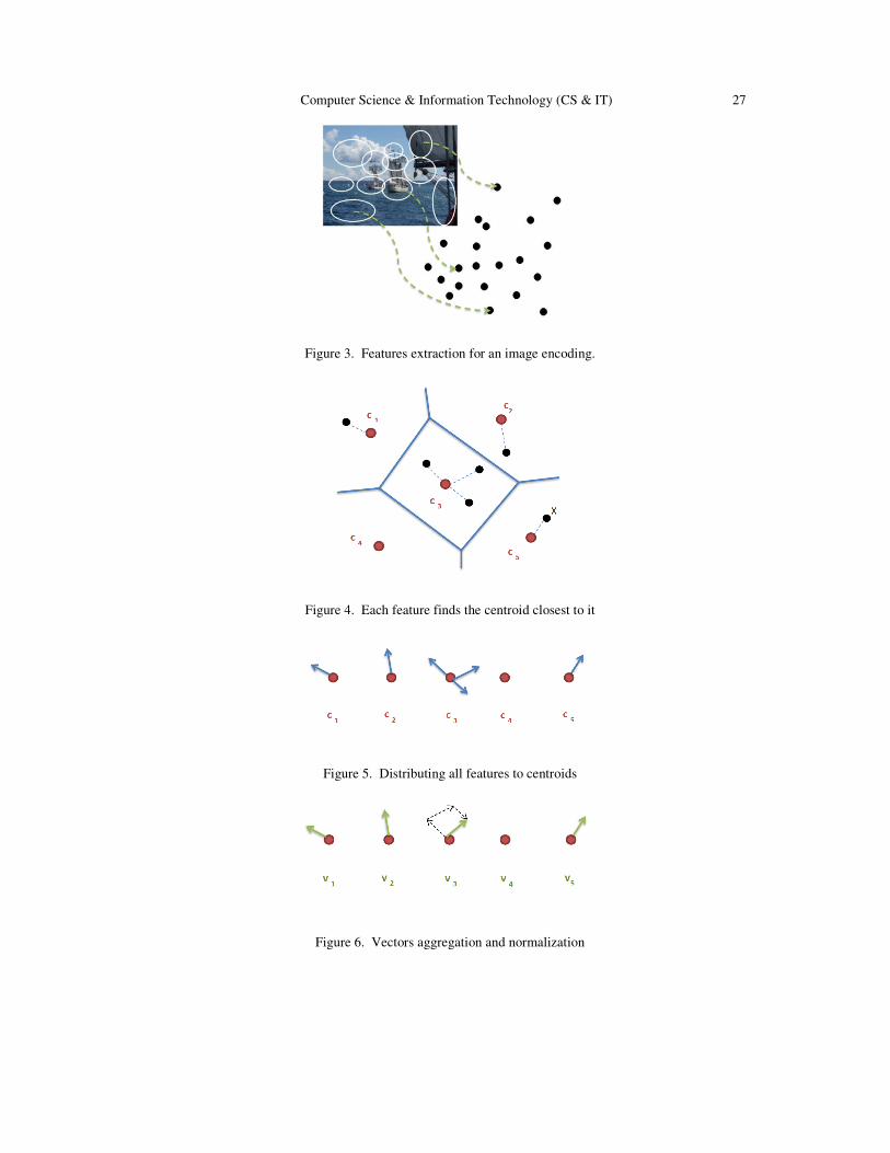
Computer Science & Information Technology (CS & IT) 27
Figure 3. Features extraction for an image encoding.
Figure 4. Each feature finds the centroid closest to it
Figure 5. Distributing all features to centroids
Figure 6. Vectors aggregation and normalization

28 Computer Science & Information Technology (CS & IT)
3. PROPOSED METHOD
3.1. Multiple Feature Extraction VLAD adopts SIFT as the feature descriptors for encoding. The state-of-the-art SIFT proposed by
Lowe[1] is a well-known feature descriptor which is widely applied in computer vision, object
recognition and machine intelligence due to its feature distinctness, robustness, and scale and
rotation invariant. For achieving higher accuracy for large scale image retrieval, this paper
proposes the scheme of integrating multiple types of feature into VLAD algorithm to enhance the
distinctness between image objects. Thus, besides SIFT, we also adopt the well-known feature
descriptors, including SURF, DAISY, and HOG. Detail of each feature descriptor is elaborated in
the following.
SURF is proposed by Bay[4] which replaces the DoG in SIFT with Haar wavelets transform to
generate the pyramid of scale space and approximates the determinant of Hessian blob detector
by an integer evaluation for efficiency. It is feasible to be used on large scale image matching for
the real-time concern. SURF descriptors can be extracted under various dimensions, for instance,
SURF-64 or SURF-128 are the SURF descriptors with dimension 64 or 128, respectively.
DAISY is a local dense feature descriptor scheme proposed by Tola[2]. Similar with SIFT, it
generates block-based orientation histogram but uses Gaussian convolution to aggregate these
blocks for efficiency. It has been shown that DAISY is a feasible and efficient feature descriptor
to be applied in wide base-line stereo matching. In this work, we uses dimension 200 to extract
DAISY descriptors.
The HOG descriptor is proposed by Dalal and Triggs[8], is a well-known feature descriptor and
widely applied in human or pedestrian detections due to its robustness of geometric shape and
luminance. It consists of three hierarchical structures, naming cell, block, and window,
respectively. The feature extraction starts by processing the image to a greyscale form, and
divides the image into several cells. Each cell is partitioned into nine bins according to the
orientation of gradients, and every four neighboring cells form a block. Then use a block to scan
the window for each step, the length of one cell at a time. Eventually, a feature descriptor is
generated by integrating feature vectors in all blocks. In this paper, we define that a cell consists
of 8*8 pixels, and four cells form a block with 16*16 pixels. The block then scans a window
consisting of 64*128 pixels for each step with length 8 pixels. Thus, every cell has nine
orientation features, and each block contains 36 features. After window scanning is completed,
we obtain (64-8)/8=7 scanning blocks in horizontal direction,and (128-8)/8=15 scanning blocks
in vertical direction. Therefore, the dimension of such a HOG descriptor is 64*7*15=3780.
3.2. Codebook Training
As aforementioned, VLAD uses k-means to cluster all SIFT features extracted from all training
images to find a certain number of centroids, the codebook. Similarly, we can extract other types
of feature descriptors, such as SURF-64, SURF-128, DAISY, and HOG from all training images
to compute the corresponding codebooks. Besides, the dimension of codebook, i.e., the number of
centroids for K-means clustering is also a crucial effect upon the accuracy of recognition. In this
paper, we train codebooks with 64 clusters, 128 clusters, and 256 clusters, respectively.
3.3. Combined VLAD Encoding
After finishing the codebooks generation, the encoding process for an image can be elaborated as
follows. An image can be computed for its VLAD encoding vector with a specific codebook. The
proposed encoding method is to combine several VLAD encoding vectors that are encoded by

Computer Science & Information Technology (CS & IT) 29
different codebooks into a normalized encoding vector. For instance, if four types of features,
SIFT, SURF-64, DAISY and HOG are adopted and the sizes of codebook are all set to 64, an
image is firstly encoded by SIFT codebook, followed by a normalization process, to produce a
VLAD encoding vector of SIFT with dimension 128*64=8192. Applying similar processes, we
can compute the normalized VLAD encoding vector of SURF-64, DAISY, and HOG for this
image, respectively. Dimensions of SURF-64, DAISY, and HOG for a single VLAD encoding
vector are 64*64=4096, 200*64=12800, and 3780*64=241920, respectively. Thus, an image can
be represented by a combined normalized VLAD encoding vector with dimension
8192+4096+12800+241920=267008.
4. EXPERIMENTAL RESULTS
The training and testing images adopted in this research are from INRIA Holiday dataset[5]。The
Holiday dataset contains 500 classes of images, and a total of 1491 images. We pick one image
from each class for testing data, and the rest are for training data. Firstly, each training image is
pre-processed by VLAD encoding with a specific combination of codebooks. The 500 testing
image are then encoded by applying the same combination of codebook. To match the testing
image with the training images, the KNN[3] algorithm is adopted to list the first 1000 ranks of
encodings of training images for each encoding of testing image, and thus the mAP(mean average
precision) value can be computed to reflect the precision of retrieval.
Table 1 shows the performance of encodings which combines different numbers of feature
descriptors from one to four types. It is obviously that mAPs are noticeably promoted as the
number of feature types and the number of centroids increases. In all combinations of any two
types of feature descriptors as shown in table 2, the combination of SIFT and DAISY performs
best. Our explanation is that SIFT and SURF are local descriptors, while DAISY and HOG
preserves a certain portion of region description. Thus, the complementary between SIFT and
DAISY can achieve more complete and detail representation of an image, and thus make each
encoding more distinguishable from others. The combination of all four types of feature
descriptors as shown in Table 3, SIFT, SURF(64), DAISY, and HOG, with 256 centroids yields
the best result and significantly promotes the mAP to 0.72.
Table 1
Feature Descriptors Dimension
64-
centroids
mAP
Dimension
128-
centroids
mAP
Dimension
256-
centroids
mAP
SIFT 8192 0.52
8
16384 0.57
4
32768 0.60
4
SIFT+SURF(64) 12288 0.57
2
24576 0.59
7
49152 0.61
9
SIFT+SURF(64)+HOG 254208 0.63
7
508416 0.66
1
1016832 0.67
1
SIFT+SURF(64)+DAISY 25088 0.66
8
50176 0.67
9
100352 0.70
1
SIFT+SURF(64)+DAISY+HO
G
267008 0.68
7
534016 0.70
7
1068032 0.72
0
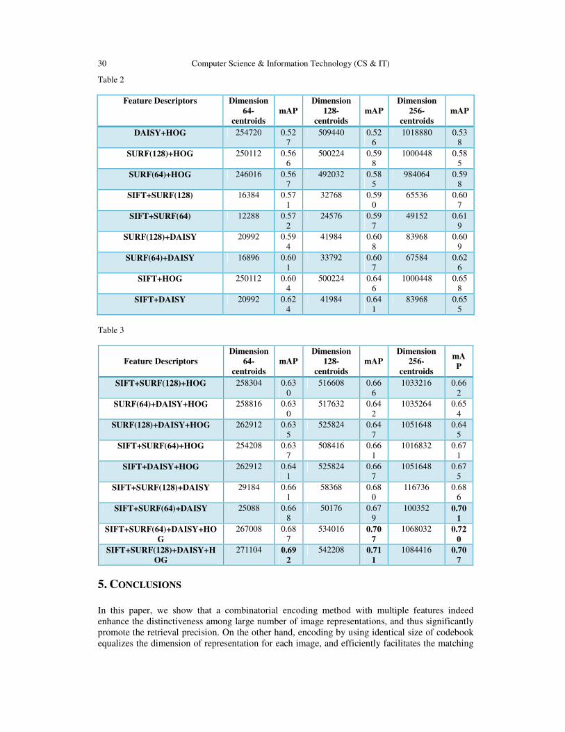
30 Computer Science & Information Technology (CS & IT)
Table 2
Feature Descriptors Dimension
64-
centroids
mAP
Dimension
128-
centroids
mAP
Dimension
256-
centroids
mAP
DAISY+HOG 254720 0.52
7
509440 0.52
6
1018880 0.53
8
SURF(128)+HOG 250112 0.56
6
500224 0.59
8
1000448 0.58
5
SURF(64)+HOG 246016 0.56
7
492032 0.58
5
984064 0.59
8
SIFT+SURF(128) 16384 0.57
1
32768 0.59
0
65536 0.60
7
SIFT+SURF(64) 12288 0.57
2
24576 0.59
7
49152 0.61
9
SURF(128)+DAISY 20992 0.59
4
41984 0.60
8
83968 0.60
9
SURF(64)+DAISY 16896 0.60
1
33792 0.60
7
67584 0.62
6
SIFT+HOG 250112 0.60
4
500224 0.64
6
1000448 0.65
8
SIFT+DAISY 20992 0.62
4
41984 0.64
1
83968 0.65
5
Table 3
Feature Descriptors
Dimension
64-
centroids
mAP
Dimension
128-
centroids
mAP
Dimension
256-
centroids
mA
P
SIFT+SURF(128)+HOG 258304 0.63
0
516608 0.66
6
1033216 0.66
2
SURF(64)+DAISY+HOG 258816 0.63
0
517632 0.64
2
1035264 0.65
4
SURF(128)+DAISY+HOG 262912 0.63
5
525824 0.64
7
1051648 0.64
5
SIFT+SURF(64)+HOG 254208 0.63
7
508416 0.66
1
1016832 0.67
1
SIFT+DAISY+HOG 262912 0.64
1
525824 0.66
7
1051648 0.67
5
SIFT+SURF(128)+DAISY 29184 0.66
1
58368 0.68
0
116736 0.68
6
SIFT+SURF(64)+DAISY 25088 0.66
8
50176 0.67
9
100352 0.70
1
SIFT+SURF(64)+DAISY+HO
G
267008 0.68
7
534016 0.70
7
1068032 0.72
0
SIFT+SURF(128)+DAISY+H
OG
271104 0.69
2
542208 0.71
1
1084416 0.70
7
5. CONCLUSIONS
In this paper, we show that a combinatorial encoding method with multiple features indeed
enhance the distinctiveness among large number of image representations, and thus significantly
promote the retrieval precision. On the other hand, encoding by using identical size of codebook
equalizes the dimension of representation for each image, and efficiently facilitates the matching

Computer Science & Information Technology (CS & IT) 31
process with KNN if compared to the traditional two-stage point-to-point and geometrical
matching processes for every pair of images. The benefits of distinctiveness and efficient
matching make it practical and feasible to apply on large scale image retrieval. Although the
dimension of encoding might increase as multiple features are applied, the computing cost caused
by large dimension can be alleviated by the novel technologies of parallel processing or
distributive computing.
ACKNOWLEDGEMENT
This project is fully supported by Ministry of Science and Technology in Taiwan under grant
number 103-2815-C-143-008-E.
REFERENCES
[1] D. Lowe. Distinctive image features from scale-invariant keypoints. IJCV, 60(2):91–220, 2004.
[2] Engin Tola, Vincent Lepetit, Pascal Fua. IEEE Transactions on Pattern Analysis and Machine
Intelligence. Vol. 32, Nr. 5, pp. 815 - 830, May 2010.
[3] Altman, N. S. An introduction to kernel and nearest-neighbor nonparametric regression. The
American Statistician. 1992.
[4] Herbert Bay, Tinne Tuytelaars, Luc Van Gool. Speeded Up Robust Features. ECCV, 2006.
[5] Herve Jegou, Matthijs Douze and Cordelia Schmid. Hamming Embedding and Weak geometry
consistency for large scale image search. ECCV, 2008.
[6] H.Jégou, M. Douze, C. Schmid, and P. Pérez. Aggregating local descriptors into a compact image
representation. CVPR, 2010.
[7] J.B. MacQueen. Some Methods for classification and Analysis of Multivariate Observations.
Proceedings of 5-th Berkeley Symposium on Mathematical Statistics and Probability, Berkeley,
University of California Press, 1967.
[8] N.Dalal and B. Triggs. Histograms of Oriented Gradients for Human Detection. CVPR, 2005.
[9] R.Arandjelovic and A. Zisserman. All about vlad. CVPR, 2013.
[10] S.Lazebnik, C. Schmid, and J. Ponce. Beyond Bags of Features: Spatial Pyramid Matching for
Recognizing Natural Scene Categories. CVPR, 2006.

32 Computer Science & Information Technology (CS & IT)
INTENTIONAL BLANK

David C. Wyld et al. (Eds) : ITCS, CST, JSE, SIP, ARIA, DMS - 2015
pp. 33–40, 2015. © CS & IT-CSCP 2015 DOI : 10.5121/csit.2015.50104
THE EFFECT OF SOCIAL WELFARE
SYSTEM BASED ON THE COMPLEX
NETWORK
Dongwei Guo, Shasha Wang, Zhibo Wei, Siwen Wang and Yan Hong
Department of Computer Science and Technology ,
Jinli University, Changchun City, China [email protected]
ABSTRACT
With the passage of time, the development of communication technology and transportation
broke the isolation among people. Relationship tends to be complicated, pluralism, dynamism.
In the network where interpersonal relationship and evolved complex net based on game theory
work serve respectively as foundation architecture and theoretical model, with the combination
of game theory and regard public welfare as influencing factor, we artificially initialize that
closed network system. Through continual loop operation of the program ,we summarize the
changing rule of the cooperative behavior in the interpersonal relationship, so that we can
analyze the policies about welfare system about whole network and the relationship of
frequency of betrayal in cooperative behavior. Most analytical data come from some simple
investigations and some estimates based on internet and environment and the study put
emphasis on simulating social network and analyze influence of social welfare system on
Cooperative Behavior .
KEYWORDS
Complex network, Welfare System, Game Theory, Cooperation
1. INTRODUCTION
At present, the game theory is widely applied in many fields such as economics, sociology and
computer science .Scientists in various fields have put forward applicable game models, such as
snowdrift game, coordination game and so on, and had good simulation results[1]. The prisoner's
dilemma model is a typical model in game theory, which interpret the process of game simple and
clear. But the prisoner's dilemma model show that individuals choose betrayal will get the highest
interest, and betrayal of dominant. However, this does not accord with actual situation, most
people need cooperation to complete something in reality. And only under the common
cooperation and the long-term relationship, the individual will achieve maximum benefit. At the
same time, because the real world not only have the individual game, but also usually a game
between people. So people often research multi-player games[2].
Complex network[3] is the research focus in the academic field in the 21st century, and it is used
in various fields to describe the relationships between all kinds of complicated things[4-5]. In
today's society, the evolution of social welfare system in the developed countries, mainly
experienced from residual welfare model to system of welfare model to hybrid welfare model
transition[6], and China's social welfare system still exist many problems, and still in the process
of perfecting. At present, most studies of social welfare system is in view of economics, there are
also many people made comparison and research between structures of national welfare system,

34 Computer Science & Information Technology (CS & IT)
but no one study the application of complex network to the social welfare system. Today's society
has formed a complex network with the person node. In this complex network, the social welfare
system for the cooperative behavior of people will produce what kind of impact? In this paper,
we combined with a complex network game model, simulate the behavior of the social individual
performance through relevant features to analysis of network status.
This paper will use the complex network to set up a social group with some orders of magnitude.
Under the natural development, Between people will influence each other and the implementation
of the welfare system and changes will affect most people in this group. when everyone is
affected and will feedback to the welfare system and affect other people around us, the people
affected with the cooperation of others will also change, may betray partners, give up
cooperation, and so on. In this big system of the dynamic and changeable, there are always Effect
and feedback. We will study such a system, and establish a model. In this model, the node
represents the individual and edge is abstracted as the relationship between the individual and
eventually form a dynamic model, to reflect the change of the whole system. And analysis how
the social welfare system based on the complex network effect on the cooperative behaviors. In
this paper, we found that let all individuals in the system to balance as soon as possible by
dynamically adjusting tax rate and the minimum guarantee of the welfare center value, and let the
wave amplitude decreases, and the network of betrayal of inhibition.
2. THE INTRODUCTION OF RELEVANT CONCEPTS
Welfare system corresponding to the social group is a social network, social network and other
natural network is also a complex system, from the social network also found the famous six
degrees of separation phenomenon (also known as the ‘small world effect).In this paper we use
the characteristics of small world network[2] to established the network model.
Welfare center: responsible for the management of the entire network, establish welfare system
(including the tax rate and poor issuance rate) of the department.
Person: the individual in the network interact with each other, with the attribute of personal id,
personal wealth, risk factor and the list of the contact.
Risk factor(SPIRIT): An individual's definition to investors, The greater the risk coefficient of
individuals tend to invest more,(0≤SPIRIT≤100).
The contact list: private property, divided into red list and white list. If the times of successful
cooperation higher than that of the number of failed, we put it into the red list, whereas in the
white list.
The blacklist: the list of the system, all people share, depositing a betrayal of people.
Rate(η): the proportion of the object charged.If the cooperation with the partner had been
success, you must pay income tax according to the specified rate.
Poor issuance rate: the proportion of the funding for poor person. Refers to the property below the
lowest life, welfare center according to its property status, issuance rate subsidies granted by
poverty.
Earnings ratio: Profit ratio when the successful cooperation.
Percentage: the ratio When failed in the cooperation.
The minimum level of consumption (min): The minimum balance individual normal life. When
individual wealth is lower than this value, welfare center will be given the allowance according to
the level of poverty

Computer Science & Information Technology (CS & IT) 35
General level of consumption(aver): the general consumption of the individual’s normal life. In
this article, we supposed that each traverse round the network through the time t, then every time
t, the property of the general individual consumption value is Aver.
Minimum value: the lowest wealth welfare center give to the poor people.
Quick deduction (δ): quick deduction =the next higher level of the highest income×(the rate at
this level -The higher tax rate) + the higher quick deduction.
3. THE INTRODUCTION OF THE SMALL WORD NETWORK MODEL
This paper uses the small world network model[2] to establish the network. Everyone can be
regarded as nodes in complex networks. There are a large number of edges connecting to the
network nodes, and two nodes connected by a line are regarded as persons who know each other.
We assume that the network had N nodes, set up steps as follows:
Step 1: Each node should be connected to K / 2 neighbor nodes around (K is even), forming the
regular net. We number N nodes of network for 1 ~ N and K lines connected to the node for 1~K.
Step 2: Whether Line 1 of node 1 would be reconnected depends on probability p (0<p<1). Node
1 of line 1 stays the same and on the other end is reconnected to other nodes of network. It meets
only a line between two points.
Step 3: Line 1 of node 2 to node N repeats step 2 until finished.
Step 4: Line 2 of node 1 to node N repeats step 2 until finished.
Step 5: Processing Line 3 to Line K of node 1 to node N by iterating until finished.
The line will never happen reconnecting while p=0 and it will be homogeneous network. The line
must be a reconnect while p=1 and it will be random network. By the introduction of Watts and
Strogatz ‘ small world network[2] in 1998, we know that small world network have characteristic
of short average path length and high degree of clustering. Let’s call degree of clustering C(p)and
average path length Iavg(P). Figure 1 shows degree of clustering and average path length is
reduced with the increase of p value, but the decreasing degree is different. It can make degree of
clustering high and average path length short while p=0.1, so this paper make p=0.1 to construct
small world network.
Figure 1. The image of degree of clustering C (red) and average path length L (blue) change with p.

36 Computer Science & Information Technology (CS & IT)
4. THE THEORETICAL MODEL
The line will never happen reconnecting while p=0 and it will be homogeneous network. This
paper is based on a small-world network to simulate real network. In the network, we define a
welfare institution and many individuals. The welfare institution manages the entire network, so
it sets rate and poor fund-issuance rate. Through simulate individual income tax in the real
society, the welfare institution taxes on profitable individuals from cooperation. If the profit is
lower than the threshold, the welfare institution wouldn’t tax. Otherwise it taxes according to the
following way
tax= taxable income × applicable tax rate quick calculation – deduction
Each time t, the welfare institution statistics its own wealth value and the wealth value it should
give out the poor people next time. When the former is lower than the latter, it will reduce the
minimum guarantee value. So this will reduce distribution of wealth value of the poor individual
and raise tax. Otherwise, if the former exceeds the latter over the continuous time 10t, it will
reduce tax and raise the minimum guarantee value. This paper starts with the minimum guarantee
value to divide poverty levels into three levels, and set different poor fund-issuance rate with the
different poverty levels. Poor fund-issuance rate is unchanged, and distribution of wealth value of
the poor individual is linearity to changes of the minimum guarantee value.
In the model, we suppose that the interaction between individuals is through investment a
comment project. Investment projects will have the risk, so according to the related factors, it
may succeed or fail. When RISK changes, GAIN and LOST along with the change. We suppose
M cooperate the same project, so
Figure 2. Formula 1
Among the above, the range of ω1 which is a random number is [-10,10], and the range of ω2
which is a random number is [0,100], and ω3 is a random number.
In this paper, we will combine the multi-player games model with single-player game. A person
can choose to cooperate with other persons who have a connection with him, ask others to invest
a project , or he can invest himself. However, individual investment would take bigger risks. In
the multi-player game, Sponsor can ask all persons who exist in the red list, part of the white list
for investing a project. But the requested people must ensure that their assets is greater than the
half of sponsor. Then the requested people can decide whether agree to cooperate by their policy
set. In the network, everyone has two alternative strategies, investment and non-investment. In
the process of cooperation, µi represents the budget investment of Node i, Pi represents expected
profit. Through the value of Pi determine whether agree to cooperation. When Pi > 0, individuals
decide to invest, otherwise individuals declined to invest. α Represents the probability of success,
Figure 3. Formula 2

Computer Science & Information Technology (CS & IT) 37
In order to maximize their own interests, individuals by their own the value of risk and the
investment situation to make their own decisions. Whether individual invest and how invest is
called the game process. The success of the investment is determined by probability. We generate
a random number between [0,100] compared with value at risk, when its value is greater than the
risk, investment success. On the other hand, investment failure. According to investment value
and earnings ratio (or loss ratio)of each investor in the project, each investor charges (or pays) the
corresponding amount. If investors cooperation successfully, investors will update their contact
list. They will put the investors they do not know before in their white list, make investment
cooperation times of investors who belong to red list to increase 1, put the investors belonging to
white list in red list and delete them from white list. If investors cooperate unsuccessfully, they
will make investment cooperation times of investors who belong to red list to decrease 1. What is
more, if investment cooperation times of investors who belong to red list are equal to 1, they will
put the investors belonging to red list in white list and delete them from red list. However, in the
process of investment a project, it may exist individual betrayal, namely , the individual will take
all the money investors invest away. Individual will be punished if they choose to betrayal. In a
period of time T (T = kt (k > 10)), it exists in the black list, individuals in the network will not
cooperate with people in the black list, and people cannot be a single investment in black list.
After a period of time, betrayers cannot cooperate with others that lead to betrayers can only
consume without income. When there is not enough wealth individuals supported the γ*t time
consumption, If individual ensure the money of investment is greater than its β times the cost of
investment and can support in T time consumption and can ensure the budget surplus amount S is
enough for their minimum consumption in the next T time, they will choose to betray. So an
individual judge whether betrayal by following condition:
Figure 4. Formula 3
Total_value means the total wealth value of investment. value(i) means the investment cost of an
individual, Self_value(i) means wealth value of an individual. Si means surplus wealth value after
an individual is deleted from the black list. θ means positive integer.
Group of betrayal by following condition:
Figure 5. Formula 4
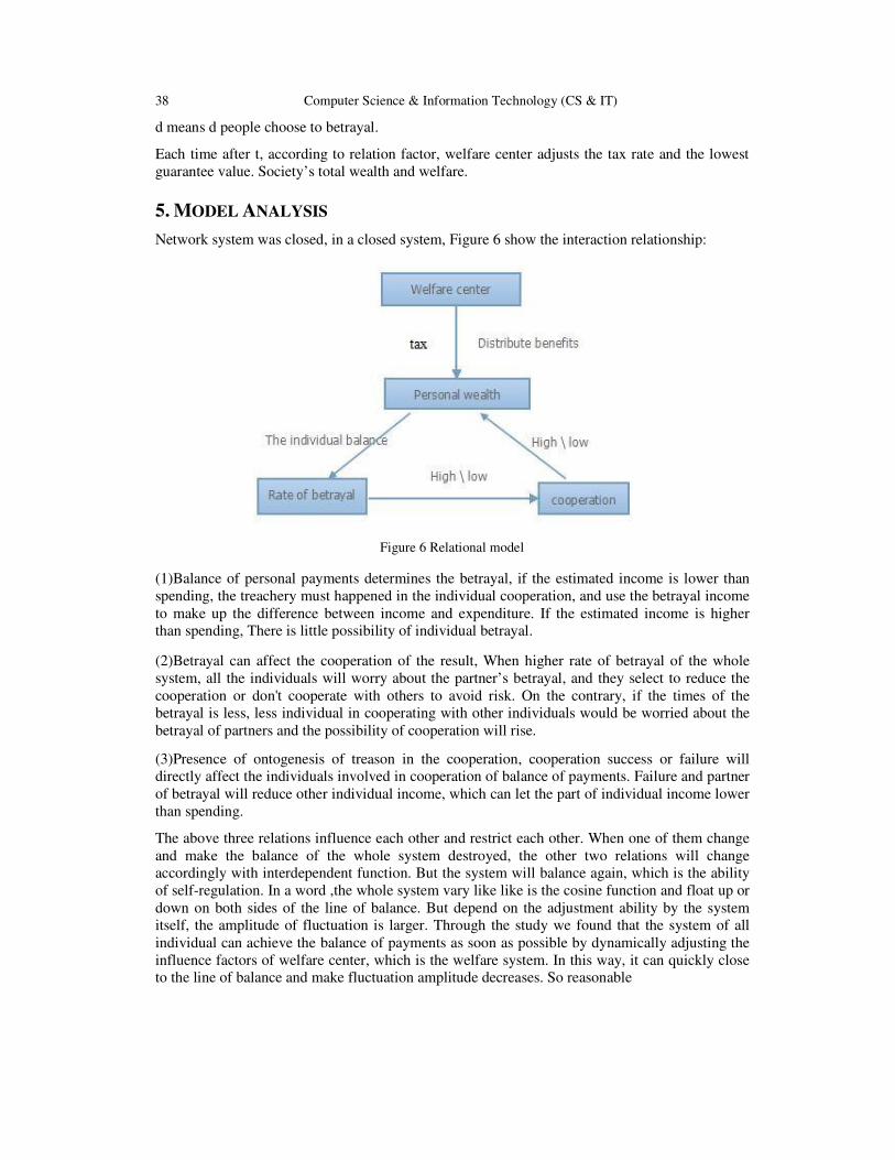
38 Computer Science & Information Technology (CS & IT)
d means d people choose to betrayal.
Each time after t, according to relation factor, welfare center adjusts the tax rate and the lowest
guarantee value. Society’s total wealth and welfare.
5. MODEL ANALYSIS
Network system was closed, in a closed system, Figure 6 show the interaction relationship:
Figure 6 Relational model
(1)Balance of personal payments determines the betrayal, if the estimated income is lower than
spending, the treachery must happened in the individual cooperation, and use the betrayal income
to make up the difference between income and expenditure. If the estimated income is higher
than spending, There is little possibility of individual betrayal.
(2)Betrayal can affect the cooperation of the result, When higher rate of betrayal of the whole
system, all the individuals will worry about the partner’s betrayal, and they select to reduce the
cooperation or don't cooperate with others to avoid risk. On the contrary, if the times of the
betrayal is less, less individual in cooperating with other individuals would be worried about the
betrayal of partners and the possibility of cooperation will rise.
(3)Presence of ontogenesis of treason in the cooperation, cooperation success or failure will
directly affect the individuals involved in cooperation of balance of payments. Failure and partner
of betrayal will reduce other individual income, which can let the part of individual income lower
than spending.
The above three relations influence each other and restrict each other. When one of them change
and make the balance of the whole system destroyed, the other two relations will change
accordingly with interdependent function. But the system will balance again, which is the ability
of self-regulation. In a word ,the whole system vary like like is the cosine function and float up or
down on both sides of the line of balance. But depend on the adjustment ability by the system
itself, the amplitude of fluctuation is larger. Through the study we found that the system of all
individual can achieve the balance of payments as soon as possible by dynamically adjusting the
influence factors of welfare center, which is the welfare system. In this way, it can quickly close
to the line of balance and make fluctuation amplitude decreases. So reasonable

Computer Science & Information Technology (CS & IT) 39
welfare system can make the system to stabilize as soon as possible, keeping society stable state.
If the welfare system is not reasonable or too light, it may have not good effect. If the welfare of
the welfare center is too much, it may be effective in a short time. But can cause negative effects
after some time, and make a lot of individuals depend on the welfare system and not participate in
cooperation, which make the welfare system’s pressure too large, and its benefits decrease. At
this time, the rate of betrayal will rebound again. Figure 7 shows the relationship between them.
Figure 7 The influence of the relationship between factors
In this picture we can see that there is no influence of the welfare system in the first stage, and the
betrayal rate of the system and the possibility of cooperation in near the equilibrium value. The
welfare system join in in the second stage. The betray in the cooperation will reduce affected by
the welfare system. Because of the reduce of the betray, the possibility of the cooperation may get
higher. In the third stage, although the welfare system continues to increase, the rate of the
betrayal reach a steady state instead of continuing to decline, the possibility of cooperation began
to fall slowly. This is due to the influence of betrayal rate in cooperation reduced or even
disappear, but the good welfare system make some individuals give up to participate in the
cooperation and depend on the welfare system. In the fourth stage, because of the magnitude of
the welfare system to achieve perfection and more people depend on the welfare system, the
welfare system was forced to cut, which can cause betrayal rate rebound and the possibility of the
cooperation will continue to decline. So a good welfare system can make the system to achieve
balance as soon as possible, and make the system stable relatively.
6. CONCLUSIONS
Welfare system can affect the speed to the balance and the amplitude of fluctuations of the whole.
Reasonable welfare system can make the overall balance quickly, reduce the amplitude of
fluctuations, and contributes to the development of the whole. On the contrary, if the welfare
system is not reasonable, it will lead to the change among the cooperation in the system larger or
smaller impact on the system.
ACKNOWLEDGEMENTS
This work was supported by the national training programs of innovation for undergraduates in
Jilin university. Then we would like to extend our sincere gratitude to our tutor Dongwei Guo for
his helpful guidance and instructive suggestions.
REFERENCES
[1] Richard Swedberg, (2001) “Sociology and game theory: Contemporary and historical perspectives”,
Theory and Society, Vol. 30, No. 3, pp301-335.
[2] Liang Chen, Shiqun Zhu, (2008) “This is my paper”, Journal of Suzhou University(Natural Science
Edition), Vol. 24, No. 3, pp55-59.

40 Computer Science & Information Technology (CS & IT)
[3] Watts DJ, Strogatz SH, (1998) “Collective dynamics of small-world networks”, NATURE, Vol.
393,No. 6684, pp440-442.
[4] Lei Guo, Xiaoming Xu,(2006) Complex Networks, Shanghai Scientific & Technological Education
Publishing House.
[5] Yongkui Liu, (2010) Study of Complex Networks and Evolutionary Game Dynamics on Networks
[D], Xi'an: Xidian University.
[6] Yingsheng Li, Yangdi Han, Yifan Xiao, Ning Zhang,(2007) “Beyond the integration model:
Classification of urban subsistence allowances system reform problem research”, Academia
Bimestris, No. 2, pp114-123.
AUTHORS
Dongwei Guo wasborn in 1972.professor, Jilin university Ph.D. Hismain research
interests include knowledge engineering and expert systems.
Shasha Wangwas born in Hebei province of China, on Sept. 19, 1993. Sheisa senior
student of Jilin University. Now her major isnetwork and information security.
Zhibo Wei wasborn in Jilin province of China, on Apr. 19,1993. Sheisa senior student
of Jilin University. Now her major isnetwork and information security.
Siwen Wang was born in Jilin province of China, on Apr. 14, 1993. Sheisa senior
student of Jilin University. Now her major isnetwork and information security.
Yan Hong wasborn in Shaanxi province of China, on Jan. 27, 1992. He isa senior
student of Jilin University. Now his major isnetwork and information security.
David C. Wyld et al. (Eds) : ITCS, CST, JSE, SIP, ARIA, DMS - 2015
pp. 41–47, 2015. © CS & IT-CSCP 2015 DOI : 10.5121/csit.2015.50105
INVENTIVE CUBIC SYMMETRIC ENCRYP-
TION SYSTEM FOR MULTIMEDIA
Ali M Alshahrani and Prof. Stuart Walker
Computer Science and Electronic Engineering,
University of Essex,
Wivenhoe Park, Colchester, Essex, UK, C04 3SQ [email protected]
ABSTRACT
Cryptography is a security technique that must be applied in both communication sides to pro-
tect the data during its transmission through the network from all kinds of attack. On the sender
side, the original data will be changed into different symbols or shapes by using a known key;
this is called encryption. On the other communication side, the decryption process will be done
and the data will be returned to its former shape by using the agreed key. The importance of
cryptography is to fulfil the communication security requirements. Real time applications (RTA)
are vulnerable for the moment because of their big size. However, some of the current algo-
rithms are not really appropriate for use with these kinds of information. In this paper, a novel
symmetric block cipher cryptography algorithm has been illustrated and discussed. The system
uses an 8x8x8 cube, and each cell contains a pair of binary inputs. The cube can provide a huge
number of combinations that can produce a very strong algorithm and a long key size. Due to
the lightweight and fast technique used in this idea, it is expected to be extremely rapid com-
pared to the majority of current algorithms, such as DES and AES.
KEYWORDS
Home of keys, Shared secret key, Encryption key, symmetric, block size.
1. INTRODUCTION
Voice, video, images, and text are examples of real time applications that need to be transmitted
quickly with a high level of security. Nowadays, there are many applications that provide real
time services, such as Skype and Tango. On the other hand, there are many suggested algorithms
that can be used to protect these applications and to guarantee that unauthorized persons cannot
access these services. Cryptography is one of the important techniques used to protect the data
during its transmit from sender to receiver by changing the situation of the message into another
shape. This process can be done in right way if both the communication sides know the key used
to encrypt/decrypt the message. DES, AES and Blowfish are examples of algorithms that deal
with the symmetric technique that is used to protect real time applications. Some of these, like
DES, are no longer used, and some of them will be broken in the coming years. Therefore, an
alternative algorithm must be implemented with a guarantee that it will fulfil all security require
ments, such as integrity, confidentiality, authentication, and non-repudiation [1]
There are two different types of cryptography: symmetric and asymmetric techniques. In this pa-
per, symmetric cryptography will be used. Symmetric key encryption, commonly called secret or

42 Computer Science & Information Technology (CS & IT)
conventional encryption, refers to the type of encryption where the keys of encryption and de-
cryption have the same values. Also, a symmetric key can contain a stream cipher and a block
cipher; the block cipher will be used here. The concept of a block cipher is to divide the text into
fairly bulky blocks, for instance, 128 bits, then encode every block individually[2][3].
The act of cracking or breaking a cipher involves extracting the plain text from the cipher text
with no knowledge of the key and frequently with no encryption algorithm information. The
strength of a cipher is evaluated according to the time required to break it, with the emphasis on
the length of time it takes to break the cipher rather than whether it is possible to break it as,
probably, all recognized ciphers except for some very few protocols, may be easily cracked or
broken[6].
Strong ciphers are those that require an extended period of time to be broken; however, they are
also likely to be more complicated and hard to apply. In contrast, weak ciphers tend to be broken
quickly; nevertheless, they are generally quite simple and uncomplicated to use. Furthermore, it is
important to take into consideration the fact that any cipher’s use has some operating expenses
concerning time and processing demands[6][7].
In recent years, a cube has been used to create some algorithms that can be used to encrypt a spe-
cific type of data (i.e. images). The main idea was to use the cube as a message container. Conse-
quently, in this paper, an 8*8*8 cube is used to generate the key that will be used to encrypt the
message.
2. LITERATURE REVIEW
The Rubik’s cube was created in 1974 for entertainment purposes. In 1992, the cube was used in
cryptography by writing and jumbling the message on the cube. It was very new technique in
cryptography and it has given rise to further new suggested techniques[13].
As mentioned previously, recently, many cryptography solutions have been implemented that use
a cube, and many of these algorithms were created for a specific type of data, that is, images. The
majority of techniques wrote the messages on the cube and then scrambled the plain text to get
the cipher text. However, the original message in this case can be obtained by anyone who can
solve the cube if the arrangement faces of the cube are known. Another disadvantage is that writ-
ing the message on the cube will help to get the plain text by linguistic analysis. This can be done
by looking for the most frequently used letter, which in the English language is ‘E’ as it is re-
peated around 12% [13][14].
A paper titled A Secure Image Encryption Algorithm based on Rubik’s Principle [15] suggests
two secret keys that are generated randomly and that take the same number of rows and columns
(M x N) as the plain text image. The technique uses the concept of a Rubik’s cube to shuffle the
pixels and then the keys will be generated by applying the bitwise XoR operation into odd and
then even rows and columns respectively, which encrypts the image. The main advantages of it
are the extreme speed and the fact that two kinds of keys are used. On the other hand, it is easy to
break because of the simple implementation. Another paper, namely, New Approach and Addi-
tional Security to Existing Cryptography Using Cubical Combinatorics [16], has a shared key that
is generated from many aspects: arrangement of letters on cube slides, arrangement of faces, ar-
rangement of colours, steps needed to reach a solved cube, and cube angle which is then ex-
changed using another existing technique. This algorithm is written with the original message on
the cube faces. The Rubik’s cube shuffles them randomly. After scrambling the cube, any known
algorithm will be applied; the authors used SHA-1 Hash. The benefits of this algorithm are that it
can be used to encrypt text and may be applied to other types of data, it is fast, and it can be com-
bined with other current and tested algorithms. However, the SHA-1 algorithm used in this tech-
nique is no longer in use. Moreover, the technique that was used to generate the key is easy to

Computer Science & Information Technology (CS & IT) 43
guess and break. The message is written on the face, and the plain text may obtained by anybody
who knows how to solve the cube, especially with the 2*2*2 cube used in their experiment.
2.1 Advanced Encryption Standard (AES):
The AES based on the block cipher symmetric encryption technique was created in 2001 and is
used by the US government as a standard. AES is considered secure and fast so most applications
use it. Its block data size is 128-bits, and it has three different key sizes: 128, 192 and 256 bits.
These different keys are generated by different numbers of rounds, that is, 10, 12 and 16 respec-
tively[6].
3. THE SUGGESTED ALGORITHM
The suggested algorithm is symmetric block cipher cryptography that is more suitable for use
with multimedia compared to the asymmetric technique because it is faster. The strongest feature
of the suggested algorithm is not the key size, although it is long, but rather is the very complex
technique used to generate the key. The possible combinations in this project are divided into two
huge numbers. One is related to the cube itself and the other one is the key length. The suggested
algorithm uses the cube to generate the key in a specific way that is completely different from the
other current algorithms. Cube 8*8*8 has a 3.6 × 10� possible number of permutations.
Moreover, the number of bits in each single cell can be 1, 2, 4 and 8 bits. 2-bits will be used in
this paper and can be represented as follows:
�: �1; 8�� ∩ ���� → �0,1��.
The key will not be exchanged. The secret shared key will be exchanged instead. The master cube
8 × 8 × 8 is a three-dimensional object limited by six square faces or sides (front, back, up,
down, right, and left faces).
In this paper, each face consists of 128 bits, and the cube’s centre facets contains of four faces
with a total of 512 bits. The whole cube has 384 cells, and each cell has 2-bits so the maximum
key length considered here is 768 or 1024 bits. The method used to mix up the home keys con-
tains complex rounds that will be used to create the EK. Actually, the rounds are divided into two
groups, and the total number of rounds is 10. The first group states the first four rounds which are
achieved by shifting the odd rows/columns by even numbers and vice versa. The second group
carries out the remaining rounds by XoR-ing each pair of faces, and stores the result in a different
face. Using fewer rounds means spending less time so all or some of the rounds can be applied.
The method of reading the cube means it is very important to specify the key length. Here, two
different ways are considered. The first method uses a face by face process as a key, starting with
128-bits for the first face and ending with 768-bits. The second reading mechanism of the cube to
obtain the 1024 bits is to read the cube’s centre facets in horizontal and vertical directions. Each
face’s cells can be shifted in 12 different directions as follows:

44 Computer Science & Information Technology (CS & IT)
Table 1: cube movement directions
Encryption Algorithm:
Encryption Algorithm: secret shared key to mix-up the key’s home and apply the se-
lected rounds.
Require 1: X is a selected block size and could be any values between 128 and 1024 bits.
Require 2: Shared Secret Key (SSK) to mix-up the key’s home. ��� = �� ∈ ^ + │1 ≤ � ≤ 7�.
Require 3: Pre-define place to hide the SSK.
1. Select the plain text (PT) size, which must be equal to the key length (K).
2. Agree shared secret key (SSK).
3. The keys’ home cube will be jumbled up by the SSK and applied to the selected rounds
(R).
4. The result of point 3 above will be the key (EK).
5. The generated key will be XoR-ed with the plain text. EK: �⨁' + ( → )*
6. The result of (5) operation will be the ciphered text: )*
7. Then, the shared secret key in point 2 above will be injected into the ciphered text in a
pre-known place: ) + ���
8. The result of 7 will be sent to the receiver: )* + ��� → (+,+-.+/.
The figure below illustrates the algorithm.

Computer Science & Information Technology (CS & IT) 45
Figure 1: Encryption process.
Decryption Algorithm:
Decryption algorithm:
Require 1: Pre-defined place to hide the SSK
The decryption process will be done in the receiver side as the following steps:
1. The receiver will receive )* + ���.
2. Then, the receiver will extract the ��� that has been hidden in a pre-defined place. As a
result, the receiver will separate the ��� from )*.
3. The ��� that is obtained from the previous point will be used to shuffle the home of the
keys.
4. The K will be produced.
5. �⨁) → '*
The figure shows the decryption process.
Figure 2: Decryption process.

46 Computer Science & Information Technology (CS & IT)
4. RESULT AND EVALUATION
Using Java, the suggested algorithm has been tested in two different packet /key sizes of 128 and
512-bits. The tested file size is 10,000 bits. Only the first group of rounds has been applied, and
the result was as follows:
Figure 1: The experiment result
From the above result, it is clear that the time needed to encrypt and decrypt the files in the sug-
gested algorithm referred to as ITU-T in its G114 recommendations was very reasonable. More-
over, it takes around a third of the time needed by AES to encrypt the files.
5. CONCLUSION
In this paper, a novel cubic symmetric block cipher technique is discussed. The greatest advan-
tages of this technique are the length of the key, the technique used to generate the key, and that
the suggested algorithm and tools are very lightweight and so are inexpensive. Moreover, the al-
gorithm can be used with all different kinds of data because it will not cause any specific delay.
Two keys are used to produce this strong algorithm. The first one is a shared key that will be used
to scramble the home keys to get the key that will be XoR-ed with the plain text. Compared to the
AES, less time is required to encrypt and decrypt the tested message. However, the delay will be
affected by the number of rounds that will be used to generate the key so it is highly recom-
mended that fewer rounds be used.
REFERENCES [1] Stinson D.,(2003), " Cryptography Theory and Practice", CRC Press Inc., NY, USA.
[2] E. Cole, R. Krutz and J. W. Conley,( 2005), " Network Security Bible", Wiley Publishing Inc,.
[3] A.D Elbayoumy, Sch. of Eng. Design & Technol., Bradford Univ, “QoS control using an end-point
CPU capability detector in a secure VoIP system”, 10th IEEE Symposium on Computers and Com-
munications (ISCC 2005).
[4] J. Evans, and C. Filsfils, Deploying IP and MPLS QoS for Multiservice Networks: Theory and Prac-
tice. Francisco: Morgan Kaufmann, 2007.
[5] A.C Rumin and E.C. Guy, “Establishing How Many VoIP Calls a Wireless LAN Can Support without
Performance Degradation,” 2nd ACM international workshop on Wireless Multimedia networking
and performance modelling, pp. 61-65, Oct. 2006.

Computer Science & Information Technology (CS & IT) 47
[6] Stallings W., (2009),“Cryptography and Network Security Principles and Practices”, Fourth Edition;
Pearson Education; Prentice Hall.
[7] Yehuda L., Jonathan K., (2007).’ Introduction to Modern Cryptography’, CRC Press.
[8] K, R. Lars, ‘The Block Cipher Companion’, Springer. ISBN 9783642173417, (2011).
[9] H. Wang ; H. Zheng ; B. Hu ; H. Tang .’’ Improved Lightweight Encryption Algorithm Based on Op-
timized S-Box’, Computational and Information Sciences (ICCIS), 2013 Fifth International Confer-
ence. Page(s): 734 - 737
[10] T. Sharma. ; R. Thilagavathy, ‘Performance analysis of advanced encryption standard for low power
and area applications’, Information & Communication Technologies (ICT), 2013 IEEE Conference,
2013 , Page(s): 967 – 972.
[11] S. Verma, R. Choubey, R. soni, ‘An Efficient Developed New Symmetric Key Cryptography Algo-
rithm for Information Security’, International Journal of Emerging Technology and Advanced Engi-
neering Web-site: www.ijetae.com (ISSN 2250-2459, Volume 2, Issue 7, July 2012).
[12] Gollmann, D. (2006), ‘Computer Security’, second edition, John Wiley and Sons.
[13] Douglas W., (1992), ‘Cryptologia’, “Rubik's Cube” As A Transposition Device’, pp. 250-256.
[14] Extended essay, ‘cryptography and Rubik’s Cube: An Investigative Analysis’, 2008.
[15] K. Loukhaoukha, J. Chouinard, A. Berdai, ‘A Secure Image Encryption Algorithm Based on the Ru-
bik’s Cube Principle’, Journal of Electrical and Computer Engineering 01/2012;
DOI:10.1155/2012/173931.
[16] P Elayaraja, M Sivakumar, ‘New Approach and Additional Security to Existing Cryptography Using
Cubical Combinatorics’, Master of Computer Applications; Dhanalakshmi College of Engineering,
Chen-nai.
[17] S. Kilaru, Y. Kanukuntla, A. Firdouse, M. Bushra & S. chava, ‘Effective and Key Sensitive Security
Algorithm For An Image Processing Using Robust Rubik Encryption & Decryption Process’, ISSN
(Print): 2278-8948, Volume-2, Issue-5, 2013.

48 Computer Science & Information Technology (CS & IT)
INTENTIONAL BLANK

David C. Wyld et al. (Eds) : ITCS, CST, JSE, SIP, ARIA, DMS - 2015
pp. 49–61, 2015. © CS & IT-CSCP 2015 DOI : 10.5121/csit.2015.50106
SVHSIEVS FOR NAVIGATION IN VIRTUAL
URBAN ENVIRONMENT
Mezati Messaoud
1, Foudil Cherif
2, Cédric Sanza
3 and Véronique
Gaildrat4
1Department of Computer Science, University of Ouargla, Algeria
[email protected] 2Department of Computer Science, University of Biskra, Algeria
[email protected] 3IRIT, Toulouse, France [email protected] 4IRIT, Toulouse, France
ABSTRACT
Many virtual reality applications, such as training, urban design or gaming are based on a rich
semantic description of the environment. This paper describes a new representation of semantic
virtual worlds. Our model, called SVHsIEVs1should provide a consistent representation of the
following aspects: the simulated environment, its structure, and the knowledge items using
ontology, interactions and tasks that virtual humans can perform in the environment. Our first
main contribution is to show the influence of semantic virtual objects on the environment. Our
second main contribution is to use these semantic informations to manage he tasks of each
virtual object. We propose to define each task by a set of attributes and relationships, which
determines the links between attributes in tasks, and links between other tasks. The architecture
has been successfully tested in 3D dynamic environments for navigation in virtual urban
environments.
KEYWORDS
Virtual environments, semantic modeling, ontology, Virtual Human
1. INTRODUCTION
Nowadays, many applications use virtual environments in different contexts such as medicine [1],
virtual heritage [2], education [3], Geographical Information Systems [4], scientific research [5],
and WorldWide Web [6]. Current virtual environment representations describe models of
environments so that browsers can effectively visualize their geometry and can support low-level
interactivity in most of cases [7][8][9]. There is a gap between the low-level representation of the
universe and how we conceptualize (and therefore how we think and talk about this universe).
Thus, a high-level model’s representation (including semantic descriptions of objects in the
environment) is desirable in order to support user interactions which are richer in a more abstract
level (querying for contents) and reasoning of deployed agents on the environments they inhabit.
1Semantic Virtual Humans In Virtual Environments

50 Computer Science & Information Technology (CS & IT)
We believe that the semantic information in virtual worlds should be considered as a component
of the universe. Therefore, the construction of virtual environments should contain semantic
annotations about the environment [7][10]. Modeling techniques are rooted in semantic
information systems, namely databases, geographic information systems, etc. Data representation
is a critical issue for these systems. Traditional approaches simply focus on techniques that
support efficient storage and retrieval of data. Otherwise, semantic modeling makes the data
meaningful, and therefore machine-readable [11]. The Semantic Web is a good example of what
semantic modeling can provideby inserting machine-readable metadata, it allows the information
stored in meaning web pages to be processed by algorithms and researches based on their content
[6].
The role of the semantic modeling of virtual environments (VEs) is to provide an abstract, high-
level and semantic description of different aspects of a VE: structure of the virtual environment,
behaviors and interactions of entities, domain knowledge, etc.[8,9]. A main motivation for adding
a semantic model is to ease the design of intelligent VEs. This intelligence of VEs mixed with
artificial agents and users can be defined as the capacity of artificial agents to exhibit human-like
behaviors and to be capable to assist users to solve a specific problem [12].
Ontologies have been used in virtual worlds as a relevant formalism to provide a conceptual
representation of scene contents. The main idea has been a direct mapping between graphical
contents and ontologies [8,11]. The concepts in an ontology can be the exact copy of the specific
graphical resources, butthis leads to several inconveniences. First, ontologies are not able to
represent entities with no graphical representation in VEs. Second, it is not possible to share
common properties among a family of graphical resources. For instance, movable objects have
some properties in common in comparison with unmovable objects.
In short, our model proposes that each virtual object in a particular virtual environment is
geometrically considered as its minimum bounding-box, and corresponds to a particular type of
object in a specific ontology. In addition, this model also establishes relationships between
elements in the VE. This model (called SVHsIEVs) uses virtual humans in VE. Each virtual
human uses both two techniques. The first technique: Guidelines, ensures coherence and
sequence of tasks. The second technique: Querying ensures the communications between agents
and ontology.
In the next section, we briefly review related works. A detail description of the proposed semantic
modeling is given in section 3. Section 4 describes the definition and the role the ontology in
VEs. The architecture of the proposed environment is illustrated in section 5. Section 6 concludes
the paper and outlines some future works.
2. RELATED WORKS
Semantic modelling techniques are rooted in Information Systems, namely Databases,
Geographical Information Systems, and World Wide Web. Data representation is a crucial issue
for these systems. Traditional approaches merely focus on techniques that promote efficient
storage and data retrieval. On the contrary, semantic modeling aims to make data meaningful and
consequently compatible with machine-process able. The semantic web is a good example of
what semantic modelling can provide. By inserting machine-readable metadata, it allows the
meaningless information stored on web pages to be processed by algorithms, which perform
researches based on their content.
This section describes several approaches and concrete works concerning the addition of a
semantic level to a virtual world, and designing of VE along with the semantic model. The

Computer Science & Information Technology (CS & IT) 51
metadata are added in the model as the objects are created. This technique has been used either
for content-oriented and system-oriented approaches, building the VE based on a pre-existent
semantic level. The main idea of this technique is to get benefits from an existing semantic
model. For instance, one can use an existing Geographical Information System to build virtual
urban environments, adding semantic annotations to the pre-existent VE[10]. The semantic
annotations can be multimedia resources, such as texts, images, sounds, and Web links. In this
case, the added information makes sense only for the user, but isnot semantically interpreted by
the system.
Cavazza & Ian [14] present technical problem in the implementation of intelligent virtual worlds,
theydeal with the need to find a knowledge representation layer. They recognize that in some
virtual world applications there is a need for the simultaneous access to concrete and abstract
information. These intelligent virtual worlds, based on theproposed common representation layer,
offer advantages regarding adaptability and reusability.
Thalmann et al [15] present an informed environment that creates a database dedicated to urban
life simulation. They introduce a method for building virtual scenes with semantic information for
the exploitation of such scenes. The three-dimensional scene provided by the designer is divided
into two parts, one for visualization and another for database construction. The database contains
geometrical and semantic information for mobile entity simulation.
Doyle [10] introduces the concept of the annotated environment, so the structured representation
of their content and their objectives are available to any agent in the environment. This
description of an agent architecture gives the possibility to interact with an annotated virtual
environment, with a structure for representing information in these environments.
Badawi& Donikian [16] describe the STARFISH (synoptic objects for tracking actions received
from interactive surfaces and humanoids) architecture that uses synoptic objects to allow real-
time object manipulation by autonomous agents in a virtual environment. A set of actions is
defined. Then these actions are assigned to interactive surfaces that definethe geometry of an
object and that are concerned by the action. The agent then uses these interactive surfaces to get
the data specific to the object when it wants to manipulate it and to adapt its behavior
accordingly.
The current trend is the use of ontologies to model the semantic information of virtual
environments. Vanacken et al [17] introduce the use of semantic information, represented using
ontologies, in conceptual modelling of interaction invirtual environments.
This semantic information itself is created during the design of the virtual world. More
concretely, semantics is incorporated in NiMMiT (Notation for MultiModal interaction
Techniques) [18], a diagram based notation intended to describe multimodal interaction. Some
works have proposed complete architectures that include a semantic layer, which is the interface
between the agents and the world. This layer usually models the world through a semantic
representation defined according to a set of ontologies. Chang et al [19] present a framework that
allows separating the agent mind from the environment. An ontology-based cognitive middle
layer between agent minds and the environment manages semantic concepts. Ontologies are
mapped onto the environment, through which characters understand the world as instances of
interconnected concepts rather than numerical values, allowing them to infer the relation between
objects. This layer also represents actions through causal rules whose effect is turning the target
object into an instance of another concept.

52 Computer Science & Information Technology (CS & IT)
With Grimaldo et al [20], an approach that uses ontologies as a basis to animate virtual
environments inhabited by intelligent virtual agents is presented. The proposed architecture is a
multi-agent framework, which can be divided into several parts: ontologies that define the world
knowledge base; a semantic layer which is the interface between the agent and the world;
planning based agents that receive sensorial information from the semantic layer and calculate the
appropriate sequence of actions in order to achieve their goals; and a 3D Engine that extracts
graphical information from the object database and performs visualization.
The ontology is consideredas a means for social relations between agents within an artificial
society. These relations must be used into account in order to display socially acceptable
decisions [21].
This approach has been used to simulate the virtual bar of a university, where groups of waiters
and customers interact with both the objects in the scene and the other virtual agents finally
displaying complex social behaviors [22].
Ibânêz et al [23] think that application approaches are necessary, and they are different from one
another in nature. Thus, the model they proposed is situated at a lower level than approaches,
which depend of applications. Their model does not intend to substitute to application dependent
approaches, but to constitute a common lower level for all of them. The authors’intention was to
create a useful model, that is, a model actually employed by the world creators. Thus, their
principle was that it should not require a great annotation effort from the environment creators.
As a result, the model consists of a reduced number of different features, and the majority of them
can be automatically annotated.
Tutenel et al [24] introduced the Semantic Class Library to design semantic VEs, notably 3D
games. After creating a 3D model, the designer associates the elements of the 3D model to
existing classes in the library. Otherwise, the designer can create a new class with the desired
properties. Beyond the 3D representations of objects within the game world, the Semantic Class
Library provides additional semantics to the objects, such as physical attributes (e.g., the mass or
material), functional information (e.g., how one can interact with an object).
3. VIRTUAL HUMAN
Lot of research has been done on behavioral animation of virtual agents over the last few years –
see [25] for a good introduction to the field. The pioneer work of [26] showed how to design a
framework to animate natural ecosystems. He simulated artificial fishes in the natural complexity
of virtual underwater worlds. However, human behavior is clearly different and more complex to
emulate. Possibly, the more relevant works in this field came from Thalmann’s group [15]. The
goal of these previous works was to design agents with a high degree of autonomy without losing
control. Their agents are an extension of the BDI architecture described in [27], and they include
internal states as emotions, reliability, trust and others. BDI-based agents have been also used in
games such as Epic Game’s Unreal [28].
Some research has been done about the questions of credibility of groups of synthetic characters,
usually centered on the interactions either among a human user and a virtual character [29] or
between virtual characters [30]
Creating Virtual Humans is a complex task, which involves several Computer Science domains:
Geometric Modeling, Computer Graphics, Artificial Intelligence, and Multimodal Interfaces [31].
In his works, Gutierrez proposed a semantics-based approach in order toorganize the different
kindsof data that constitute a Virtual Human.
Computer Science & Information Technology (CS & IT) 53
The knowledge defined by the synthesis, functionalities and animation of VHs is formally
specified by the way of ontology. This approach is similar to our purpose in the section 4.2.
4. ONTOLOGY IN VIRTUAL ENVIRONMENT
Virtual Humans are virtual entities with a rich set of functionalities and potential, present in a VE.
One of the main instruments used to lay-down the foundations of a knowledge-based system are
ontologies. Ontology defines a common vocabulary for domain-users (researchers or experts in a
particular area) who need to share information in a particular domain. It includes machine-
interpretable definitions of basic concepts in the domain and relations among them. The
semantics-based representation can be enhanced by means of knowledge-management techniques
and tools. One of the main tools used to lay-down the foundations of a knowledge-based system
is therefore an ontology. A first one focuses on the adaptive multimodal interfaces system and a
second one formalizes the knowledge related to the creation of virtual humans and serves as a
basis for a general ontology for Virtual Environments [32]. Many consider W3C’sWeb Ontology
Language (OWL) the prospective standard for creating ontologies on the Semantic Web.
OWL has three species: OWL Lite, OWL DL and OWL Full, in ascending order according to
expressiveness. We can divide the use of ontologies in thedomain of Virtual Environments into
three uses; the first use: Ontologies in the context of Virtual Environments [33,34], the second use
: Ontology for interactive Virtual Environments[35,36], the third use: Ontology for Virtual
Humans [31,37].
5. OUR FRAMEWORK (SVHSIEVS)
In the framework SVHsIEVs, we attempt to apply the influence of the integration semantic layer
in virtual worlds. This semantic layer is distributed according to two levels. The first level is
global, in this level we can define semantic information on a more global way. The second level
concerns the virtual objects; in this level, objects need to transcend the geometry concepts and
more abstract information need to be incorporated into the object’s description. Many properties
of real-world objects should be represented in their virtual counterparts to allow an algorithm to
perform some kind of reasoning on objects (e.g., the physical attributes define whether or not the
object is too heavy to carry, or the functional information is necessary to decide if an AI character
can use the object to reach a goal).
In our proposal semantic information use the ontology to describe the concepts used in the
domain along with their properties and relations between them, in each two levels.
Our first contribution is to show the influence of adding semantic information (contextual
attributes and relationships between concepts) to virtual objects and with the aim to use this
information to define and redefine interaction with environment.
Our second contribution concerns the use in our modelofVirtual Humans two technics: Querying
and Guidelines.
Our third contribution concerns the use of this semantic information in management of tasks for
each virtual object; we propose to define each task by more attributes and set of relationships, this
relationships determine on one side the links between the attributes in a task and on the other side
they determine the relations between tasks.
As discussed earlier in this paper, the proposed framework is based on the integration of
semantics information in virtual environment, and we show this integration in different layer.

54 Computer Science & Information Technology (CS & IT)
Also, for each objet in the environment composed of two aspects: geometry and semantic, the
aspect semantic is based on contextual information only but using the relationship between
different concepts, these concepts are present information’s semantics of different objects in
virtual environment.
In this paper we present a Semantic Virtual Environment approach that uses ontologies as an
appropriate basis to animate virtual environments inhabited by intelligent virtual Humans. Figure
1 show the architecture of our multi-agent framework, which can be divided into several parts:
Ontologies define the world knowledge base as well as the set of all possible relations among the
agents and virtual humans. We distinguish two levels of representation: the SVE Core Ontology
is a unique base ontology suitable for all virtual environments which can be extended by different
Domain Specific Ontologies in order to model application-specific knowledge. Then,
environments can be constructed by instantiating the classes of these ontologies. For example, in
section Implementation we will create pedestrians a virtual city with a large number of objects –
cars, crossroads, etc.
Figure 1. SVHsIEVs architecture
The Semantic Layer is the interface between the virtual human and the world. It uses the ontology
so as to reduce the information flow; this layer is in charge of executing the actions requested by
the agents as well as maintaining their semantic effects.
In the structure of Virtual Human we find the combination between three aspects: Virtual human
intelligent (VHI), Querying and Guidelines. The VHI insures the intelligent interaction with
world and the others VHI and the querying insures communication (asks and answers) with the
world. The Guidelines insures the planning of different tasks.
5.1 Ontology of virtual environment
The goal of ontology design for virtual environment in this architecture is two parts. First, we
would like to keep the information that exists in the virtual environment such as object geometry
and transformation. Second, we use semantic information about the virtual objects can facilitate
the computation of advanced reasoning procedures such as a navigation in the world.
Our ontology design of the virtual environment is shown in Figure 2. The root of the ontology is
the environment node, which contains world information (environment) and all the virtual objects
(object) in the environment. In order to retain the semantic information of the virtual objects, we
have designed the base Info and Transform nodes; in this node we show sub-information as
position and rotation. Each object also has some additional attributes such as name, weight, height
and tag. All this attributes are designed for public properties for virtual objects. For example, the

Computer Science & Information Technology (CS & IT) 55
urban environment, one can tag certain objects as s pedestrian area and car area such that these
regions can be treated appropriately by the urban environment according to their meanings in the
world. Each object in environment as (building, car and Column lights…) may also have the
attribute of Approximation 3D, which is a polygon that can be used to define 3D approximation
of obstacles in the environment for the navigation.
Figure 2. Ontology design for virtual environment
5.2.VHs architecture
The Virtual Human is based on three aspects; Virtual human intelligent (VHI), Querying and
Guidelines. The VHI gives the intelligent interaction with world and other VHI and the querying
gives asks and reception the answers with world. The Guidelines gives the pacification of
different tasks.
The module gives the aspect querying, it is a communication module, and in this module we show
two types of communication: the first protocol with other Virtual Human by message for example
demand the service or information, the second protocol with environment by the queries. The
answer of these queries is divided into two cases according to natural answer; if the answer is a
static information like position or direction by example, in this case, the answer is simple
processing; we take the query and search in the ontology of data information without treatment.
In second case, we use different modules as reasoning module and ontology.
Figure 3. A Virtual Human architecture
We show the aspect of guidelines in planning module, this module is ensuring the planning of
different tasks; in this part we using ontology for giving all information’s of each task, because

56 Computer Science & Information Technology (CS & IT)
each information, it is influence in the order between tasks. For example we have four tasks T1,
T2, T3 T4, with the following planning.
Figure 4. The sequence of tasks
We note that T2 and T3 are independent; in this case the order is not important. By adding more
information as the nature task such as the time attribute for example, this task is joined with time
or not; T2 is the task “buy in the store” and T3 is the task “buy in internet”; therefore, we run T2
before T3 because T2 depends on the opening of the store.
The reasoning module it is means of present the intelligent, this module likes with all reasoning
tasks for each virtual human; we show the experience or information’s of finding the path
between two points in the network of points after the Transformation the points network for VE
into form « case base ».(as shown in Figure 5)
Figure 5. Transformation the points network for VE into form « case base »
The path between two points is the sequence of sub-paths, result of the induction algorithm on the
case base.
In other case; if VH cannot get the solutions, because these information do not exist in his
ontology, it sends the query to environment or other VH to get this information. This asks is
assumed by the querying module. According to the following figure:

Computer Science & Information Technology (CS & IT) 57
Figure 6. The internal handling of requests to VHs
5.3. Ontology design for Virtual Human
In our architecture, a VH has ontology, in this ontology we describe the basic ontology classes
and attributes (as shown in Figure 7) that we have designed for the applications of the VH
navigations. Although a VH is also an object in a virtual environment, they have more active and
complicated roles to play. For example, a user in Anthropometry Description set attributes as
Height, Wight, Age, Gender, Speed and Acuity. A VH may contain some basic attributes such as
name, Transform, and status. We also take the Tired and stress for present the influence of these
properties in speed and acuity of VH.
Figure 7. Ontology design for VH
5.4 Implementation and results
We have implemented our model in Unity3D; developed in C#. We built our ontologies using the
Protégé and Jena for update. Access to the ontology is obtained by sending SPARQL queries. In
this section, we will give two examples of using semantic information in the virtual world to
enhance the functions and behaviors of the VH.

58 Computer Science & Information Technology (CS & IT)
We distinguish that the navigation of a VH in virtual urban environment is based on more tasks,
among these tasks are collision detection; avoidance of collisions and search of goals. In the two
first tasks, we use the two attributes speed and acuity, dynamically changing, because they are in
relation with other attributes (tired, stress, age, etc.).
In figures 8, we show the influence of age on speed and acuity. We distinguish three phases: the
first phase increases the speed and acuity when the age increases. The second phase is almost
stability of speed and acuity between 20 and 40 years. The last phase, after 40, decreases the two
parameters.
Figure 8. The influence of age factor on speed and acuity
Figure 9. The influence of tiredness factor on speed and acuity
Figure 10. The influence of stress factor on speed and acuity
In figure 9, we add another factor, the tiredness to test the influence of this tiredness attribute on
VH’s speed and acuity. We show the inverse relationship between tiredness and speed; the speed
and acuity decreases with increase of tiredness.
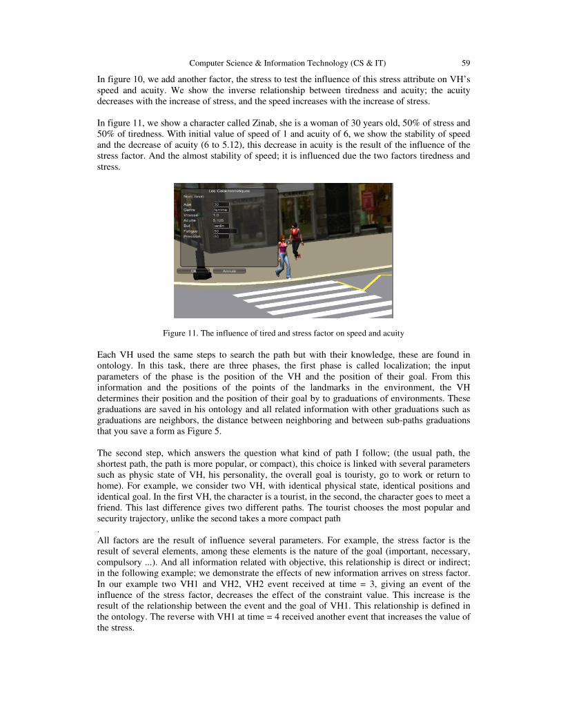
Computer Science & Information Technology (CS & IT) 59
In figure 10, we add another factor, the stress to test the influence of this stress attribute on VH’s
speed and acuity. We show the inverse relationship between tiredness and acuity; the acuity
decreases with the increase of stress, and the speed increases with the increase of stress.
In figure 11, we show a character called Zinab, she is a woman of 30 years old, 50% of stress and
50% of tiredness. With initial value of speed of 1 and acuity of 6, we show the stability of speed
and the decrease of acuity (6 to 5.12), this decrease in acuity is the result of the influence of the
stress factor. And the almost stability of speed; it is influenced due the two factors tiredness and
stress.
Figure 11. The influence of tired and stress factor on speed and acuity
Each VH used the same steps to search the path but with their knowledge, these are found in
ontology. In this task, there are three phases, the first phase is called localization; the input
parameters of the phase is the position of the VH and the position of their goal. From this
information and the positions of the points of the landmarks in the environment, the VH
determines their position and the position of their goal by to graduations of environments. These
graduations are saved in his ontology and all related information with other graduations such as
graduations are neighbors, the distance between neighboring and between sub-paths graduations
that you save a form as Figure 5.
The second step, which answers the question what kind of path I follow; (the usual path, the
shortest path, the path is more popular, or compact), this choice is linked with several parameters
such as physic state of VH, his personality, the overall goal is touristy, go to work or return to
home). For example, we consider two VH, with identical physical state, identical positions and
identical goal. In the first VH, the character is a tourist, in the second, the character goes to meet a
friend. This last difference gives two different paths. The tourist chooses the most popular and
security trajectory, unlike the second takes a more compact path
.
All factors are the result of influence several parameters. For example, the stress factor is the
result of several elements, among these elements is the nature of the goal (important, necessary,
compulsory ...). And all information related with objective, this relationship is direct or indirect;
in the following example; we demonstrate the effects of new information arrives on stress factor.
In our example two VH1 and VH2, VH2 event received at time = 3, giving an event of the
influence of the stress factor, decreases the effect of the constraint value. This increase is the
result of the relationship between the event and the goal of VH1. This relationship is defined in
the ontology. The reverse with VH1 at time = 4 received another event that increases the value of
the stress.

60 Computer Science & Information Technology (CS & IT)
Figure 12. Evolution stress factor with time
6. CONCLUSION AND FUTURE WORKS
Using semantic information’s is a key function for enabling richer contents and behaviors in the
future development of virtual environment. The SVHsIEVshave presented a semantic-based
framework for the virtual environment with Virtual Humans (VHs), our first parts integrated the
VH in virtual environment with more semantic information, these information are helping of
developing area of research that integrates computer graphics and artificial intelligence solutions.
Our second parts to show the influence of adding semantic information (contextual attribute and
relationships between their concepts) to virtual Human and using this influence for define and
redefine his interaction with environment.
Throughout the paper, we showed the importance of semantics when modelling dynamic virtual
environments. Furthermore, the VH extracted from the ontology allows the VHs to reuse their
information in different contexts. We will add different animation components owned by different
VHs to interact with each other, will integrate more semantic information for tasks and using
these information in planning phase, will implementSVHsIEVswith other environment as theatre
for example and using motions information’s as mean of communication between VHs.
REFERENCES
Short Biography
Mezati Messaoud is a Ph student at University of Ouargla since 2009. He works in the
LESIA Laboratory Biskra University. His current research interest is in artificial
intelligence, artificial life, crowd simulation, behavioral animation and virtual characters.
Foudil Cherif is an associate professor in the department of Computer Sciences at Biskra
University and head of LESIA Laboratory. He received his Phd in computer science from
Biskra University in 2006. His first underground degree is Engineer in computer science
from University of Constantine, Algeria in 1985. He received his Msc in computer science
from Bristol University, UK in 1989. His researches focus primary on Behavioural
animation, Crowd simulation, Autonomous agents, Artificial life, Artificial intelligence and
software engineering.

Computer Science & Information Technology (CS & IT) 61
Cédric Sanza earned his Ph. D. in 2001 and he is a research lecturer at University of
Toulouse since 2002. He works in the field of simulation of virtual characters. He mainly
focuses on physical motion and behavioral systems to design autonomous entities in 3D
worlds. He is also interested in learning by imitation in classifier systems to automatically
build complex behaviors.
Véronique Gaildrat is a full professor in the department of Computer Sciences at
University of Toulouse since 2007. She is member of the IRIT laboratory (Institut de
Recherche en Informatique de Toulouse) where she works in the field of declarative
modeling of virtual environments. Lately she worked in the field of theater, in order to
automatically create a virtual scenography based on the author's text, including
representation of the emotional state of virtual actors.

62 Computer Science & Information Technology (CS & IT)
INTENTIONAL BLANK

David C. Wyld et al. (Eds) : ITCS, CST, JSE, SIP, ARIA, DMS - 2015
pp. 63–70, 2015. © CS & IT-CSCP 2015 DOI : 10.5121/csit.2015.50107
ON DIAGNOSIS OF LONGWALL SYSTEMS
Marcin Michalak, Magdalena Lachor
Institute of Informatics, Silesian University of Technology, Gliwice, Poland {Marcin.Michalak,Magdalena.Lachor}@polsl.pl
ABSTRACT
Nowadays we can observe the change of the structure of energy resources, which leads to the
increasing fraction of a renewable energy sources. Traditional underground coal mining loses
its significance in a total but there are countries, including Poland, which economy is still coal
based. A decreasing coal resources imply an exploitation a becoming harder accessible coal
beds what is connected with the increase of the safety of the operation. One of the most
important technical factor of the safety of underground coal mining is the diagnostic state o a
longwall powered roof support. It consists of dozen (or hundreds) of units working in a row. The
diagnostic state of a powered roof supports depends on the diagnostic state of all units. This
paper describes the possibility of unit diagnostic state analysis based on the biclustering
methods.
KEYWORDS
Biclustering, Longwall Systems, Machine Diagnosis.
1. INTRODUCTION
In a coal mining industry – similarly as in the case of other industry branches – the growth of
monitoring systems application. Initially, monitoring systems were designed just for the purpose
of data acquisition and presentation. Over time, their abilities were extended in the direction of
simple dangerous situations recognition and finally – to the advanced machine diagnostic status
analysis and its prediction for the nearest future.
Longwall systems are the basis of the coal mining, because the longwall is the place in the
process of mining from which we can say about the output. Mechanised longwall systems consist
of longwall shearer (which tears off the output from the rock), longwall conveyor (transports the
output from the longwall to the heading) and units of powered roof support (prop the roof after
mining the output).
Longwall systems are very interesting objects from the collected data point of view. Its most
important part is a power roof support. Its primary task is to protect the other elements of the
longwall system, especially the coal shearer which is an essential part as of a coal mining process.
Power roof support consists of units. In a particular moments of time – after shearer takes the
another part of the longwall output – each unit has to move in the direction of the whole longwall
face advance (treading), protecting the rock material, exposed by the shearer, from collapsing.
Unequal propping can be caused by leaks in the hydraulic system (pipes, valves) or leaks in legs
of the unit. To long times of treading can point the wrong diagnostic state of the unit or be caused
by the wrong usage (so called: moving with the contact of roof-bar with the roof). It is also
dangerous to perform the treading too long as the roof is not propped. So it can be stated that the

64 Computer Science & Information Technology (CS & IT)
safety of coal mining is determined by the diagnostic state of all parts of the longwall mining
system, including the diagnostic state of all units of power roof support.
In this article the ability of adaptation of biclustering method for the purpose of the analysis the
data from longwall monitoring systems is presented. The paper is organized as follows: it starts
from the brief description of monitoring systems with a special consideration of underground coal
mining monitoring system is presented. Than the description of a construction, the role and a
working cycle of a powered roof support is presented together with the proposed monitored (and
extracted) parameters. Next part presents a wide group om continuous and binary data
biclustering methods. The paper ends with a perspective of application of these methods in the
longwall monitoring systems.
2. MONITORING SYSTEMS
Nowadays, software producers and monitoring systems users point the need of analysis of the
data, collected in repositories of these systems. In particular, the definition of diagnostic models
of monitored devices can be a goal of this analysis [1][10][19]. The process of a diagnostic model
identification can be carried out by planned experiments or on the basis of a data from the past
device operation.
The problem of a monitoring and diagnosing of a coal mine industry devices was raised recently
in [1][6][8][16][17][19]. These topics are presented widely and review in [1][19]. In these works
also new methods of extraction and processing of new diagnostic features in new diagnostic
relations discovering are presented. Especially in [1] the diagnostic of conveyor belts is described.
In [17] a current consumption and a temperature of roadheader cutting head. On the basis of these
parameters three roadheader working states were defined. Two of them described different but
correct underground mining conditions. In this paper also the parameter reflecting the roadheader
cooling system efficiency was defined.
Longwall conveyors diagnostic was an aim of the following works [6][8][16][4][5][12]. In [6]
the way of conveyor chute failures detection on the bottom side of a conveyor was presented. On
the basis of the conveyor engines power consumption analysis the failure was detected with an
accuracy to the one unit. In [8] the complex subassemblies management system was proposed,
which allows to generate operational and analytical reports as well as summary statements.
In [16] the analysis of the motor driving the conveyor power consumption is described. As the
result summary reports are presented and an association rules-based description of the motor
operating parameters are described.
3. POWERED ROOF SUPPORT
The safety of underground coal mining depends on many of natural and technical factors, also
including the human factor. From the technical factors the diagnostic state of powered roof
support units must be acknowledged. It becomes more understandable when the construction and
the working cycle of single unit is known. In this section the basics of the powered roof support
unit structure and its working cycle description are presented.
3.1. Unit Structure
An unit consists of one or more hydraulic prop (legs), holding up an upper part of the unit (roof-
bar). It also has and hydraulic shifting system that is responsible for shifting the unit with the
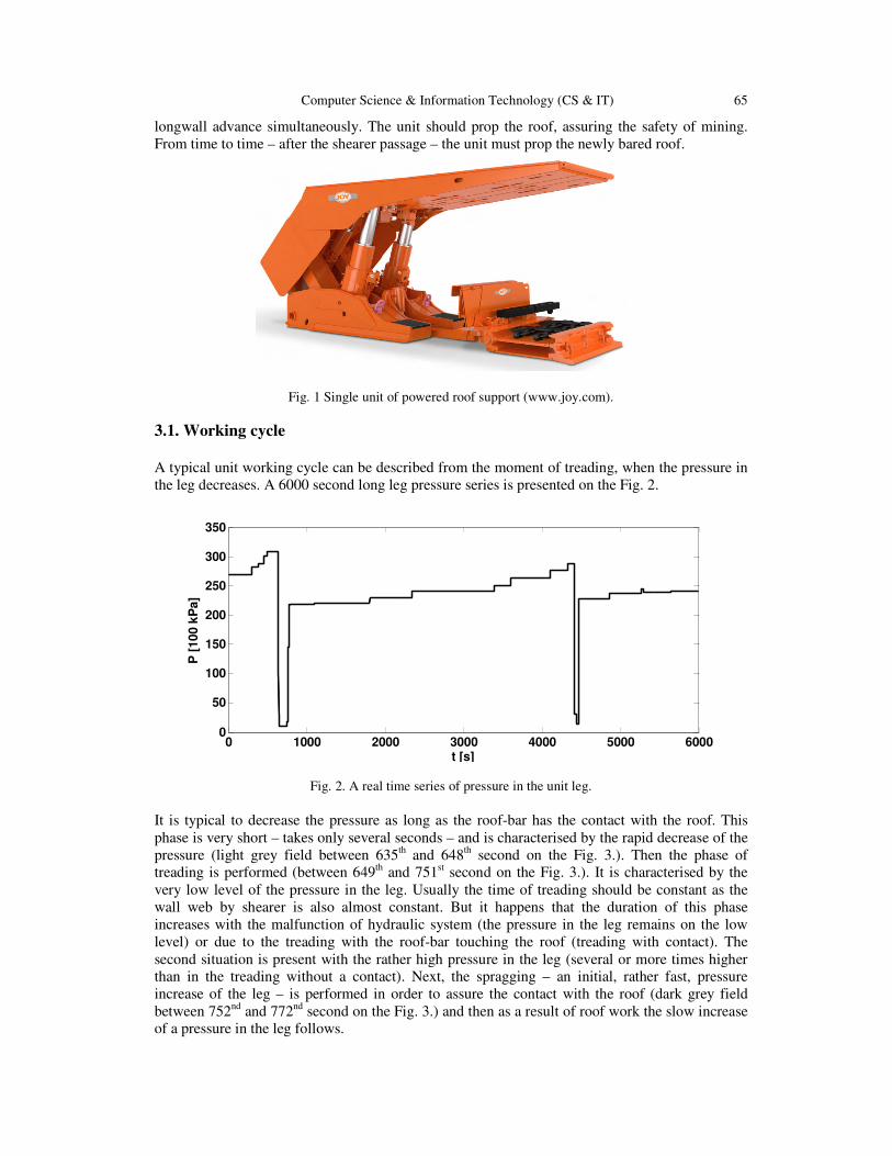
Computer Science & Information Technology (CS & IT) 65
longwall advance simultaneously. The unit should prop the roof, assuring the safety of mining.
From time to time – after the shearer passage – the unit must prop the newly bared roof.
Fig. 1 Single unit of powered roof support (www.joy.com).
3.1. Working cycle
A typical unit working cycle can be described from the moment of treading, when the pressure in
the leg decreases. A 6000 second long leg pressure series is presented on the Fig. 2.
Fig. 2. A real time series of pressure in the unit leg.
It is typical to decrease the pressure as long as the roof-bar has the contact with the roof. This
phase is very short – takes only several seconds – and is characterised by the rapid decrease of the
pressure (light grey field between 635th and 648
th second on the Fig. 3.). Then the phase of
treading is performed (between 649th and 751st second on the Fig. 3.). It is characterised by the
very low level of the pressure in the leg. Usually the time of treading should be constant as the
wall web by shearer is also almost constant. But it happens that the duration of this phase
increases with the malfunction of hydraulic system (the pressure in the leg remains on the low
level) or due to the treading with the roof-bar touching the roof (treading with contact). The
second situation is present with the rather high pressure in the leg (several or more times higher
than in the treading without a contact). Next, the spragging – an initial, rather fast, pressure
increase of the leg – is performed in order to assure the contact with the roof (dark grey field
between 752nd
and 772nd
second on the Fig. 3.) and then as a result of roof work the slow increase
of a pressure in the leg follows.
0 1000 2000 3000 4000 5000 60000
50
100
150
200
250
300
350
t [s]
P [
10
0 k
Pa
]

66 Computer Science & Information Technology (CS & IT)
3. POWERED ROOF SUPPORT
The most important element of powered roof support monitoring is the measuring legs pressures
in each unit. This helps to determine the working cycle phase of unit. Following also the durations
of all cycle phases can be calculated, including the treading time. For units equipped with more
than one leg also the effective roof propping strength can
propping may have negative consequences influencing on the unit diagnostic state.
On the basis of measured pressures in all units in the longwall the detailed analysis of each unit
work and even each leg in the unit work du
following aspects:
- Durations of unit working cycle phases,
- Pressure statistics aggregated in time intervals (max, min, std)
- Inequality of propping (for units with two or more legs)
- Statistics of treads (durations, pressure level)
As all characteristics are time dependent (values are varying in the time) and all units can be
treated as objects from the same population, every characteristic for the powered roof support can
be present as the twodimensional matrix.
that the time axis is the X axis we will assumed that following sections are rows and the column
represents the state of all units at the selected time in the past.
This matrix can be interpreted as the image in the further analysis, but this assumption implies
that two distant units which behave in the same inappropriate way should be considered
separately. In our feeling this does not reflect the nature of the proce
twodimensional data analysis is searching of subsets of rows which behave in the similar way on
the subset of columns. This way of data analysis is called biclustering.
Computer Science & Information Technology (CS & IT)
Fig.3. Phases of unit working cycle.
UPPORT MONITORING
The most important element of powered roof support monitoring is the measuring legs pressures
in each unit. This helps to determine the working cycle phase of unit. Following also the durations
of all cycle phases can be calculated, including the treading time. For units equipped with more
than one leg also the effective roof propping strength can be determined. Unequal roof
propping may have negative consequences influencing on the unit diagnostic state.
On the basis of measured pressures in all units in the longwall the detailed analysis of each unit
work and even each leg in the unit work during the exploitation can be performed, including the
Durations of unit working cycle phases,
Pressure statistics aggregated in time intervals (max, min, std)
Inequality of propping (for units with two or more legs)
(durations, pressure level)
As all characteristics are time dependent (values are varying in the time) and all units can be
treated as objects from the same population, every characteristic for the powered roof support can
al matrix. A sample matrix is presented on the Fig. 3. It is intuitive
that the time axis is the X axis we will assumed that following sections are rows and the column
represents the state of all units at the selected time in the past.
This matrix can be interpreted as the image in the further analysis, but this assumption implies
that two distant units which behave in the same inappropriate way should be considered
separately. In our feeling this does not reflect the nature of the process. The other way of
twodimensional data analysis is searching of subsets of rows which behave in the similar way on
the subset of columns. This way of data analysis is called biclustering.
The most important element of powered roof support monitoring is the measuring legs pressures
in each unit. This helps to determine the working cycle phase of unit. Following also the durations
of all cycle phases can be calculated, including the treading time. For units equipped with more
be determined. Unequal roof-bar
On the basis of measured pressures in all units in the longwall the detailed analysis of each unit
, including the
As all characteristics are time dependent (values are varying in the time) and all units can be
treated as objects from the same population, every characteristic for the powered roof support can
. It is intuitive
that the time axis is the X axis we will assumed that following sections are rows and the column
This matrix can be interpreted as the image in the further analysis, but this assumption implies
that two distant units which behave in the same inappropriate way should be considered
ss. The other way of
twodimensional data analysis is searching of subsets of rows which behave in the similar way on

Computer Science & Information Technology (CS & IT)
Fig. 3 Matrix representing a series of legs pressures in the p
3. BICLUSTERING
Biclustering is the problem of unsupervised data analysis, where we are grouping scalars from the
two-dimensional matrix. It called also as co
clustering. This approach has been started in 70’s in the last century [7] and is successfully
applied in bioinformatics [5][14][19] or text mining [5]. The illustration of the main idea of
biclustering is presented on Fig. 1.
Fig. 4 Schematic representation of clustering (
In the literature there are a lot of algorithms of biclusters induction. In [5] authors define bicluster
as a subset of rows under subset of columns, for which calculated parameter (mean squared
residue score) is below threshold defined by the user. The mi
parameter is 0. The algorithm consists of two steps. Initially the rows and columns are removed
from input dataset, until the value of mean squared residue score is below assumed level. Then
rows and columns, which were remove
previous step submatrix until its score fulfils the criterion of being bicluster. After each iteration,
the founded bicluster has been hidden with random values. The extension of this algorithm
proposed in [20] allows to avoid noise among input dataset, which was a consequence of masking
discovered biclusters. The Order Preserving Submatrix Algorithm was presented in [3]. The
Computer Science & Information Technology (CS & IT)
Matrix representing a series of legs pressures in the powered roof support.
Biclustering is the problem of unsupervised data analysis, where we are grouping scalars from the
dimensional matrix. It called also as co-clustering, two-dimensional clustering or two
h has been started in 70’s in the last century [7] and is successfully
applied in bioinformatics [5][14][19] or text mining [5]. The illustration of the main idea of
biclustering is presented on Fig. 1.
Fig. 4 Schematic representation of clustering (left, centre) and biclustering (right) [1].
In the literature there are a lot of algorithms of biclusters induction. In [5] authors define bicluster
as a subset of rows under subset of columns, for which calculated parameter (mean squared
residue score) is below threshold defined by the user. The minimum value of the considered
parameter is 0. The algorithm consists of two steps. Initially the rows and columns are removed
from input dataset, until the value of mean squared residue score is below assumed level. Then
rows and columns, which were removed during the first step, are added to obtained in the
previous step submatrix until its score fulfils the criterion of being bicluster. After each iteration,
the founded bicluster has been hidden with random values. The extension of this algorithm
in [20] allows to avoid noise among input dataset, which was a consequence of masking
discovered biclusters. The Order Preserving Submatrix Algorithm was presented in [3]. The
67
owered roof support.
Biclustering is the problem of unsupervised data analysis, where we are grouping scalars from the
dimensional clustering or two mode
h has been started in 70’s in the last century [7] and is successfully
applied in bioinformatics [5][14][19] or text mining [5]. The illustration of the main idea of
left, centre) and biclustering (right) [1].
In the literature there are a lot of algorithms of biclusters induction. In [5] authors define bicluster
as a subset of rows under subset of columns, for which calculated parameter (mean squared
nimum value of the considered
parameter is 0. The algorithm consists of two steps. Initially the rows and columns are removed
from input dataset, until the value of mean squared residue score is below assumed level. Then
d during the first step, are added to obtained in the
previous step submatrix until its score fulfils the criterion of being bicluster. After each iteration,
the founded bicluster has been hidden with random values. The extension of this algorithm
in [20] allows to avoid noise among input dataset, which was a consequence of masking
discovered biclusters. The Order Preserving Submatrix Algorithm was presented in [3]. The

68 Computer Science & Information Technology (CS & IT)
bicluster was defined as subset of rows, which preserves linear ordering across subset of
conditions. The set of valid biclusters is identifying by algorithm based on stochastic model. This
idea was also evolved in [9].
The algorithm X-Motif is dedicated to the extraction of conserved gene expression motifs from
gene expression data and has been proposed in [13]. Bicluster is defined as subset of genes, which
expression level belong to the same state across subset of conditions. The states are assigned to
genes during preprocessing step. In order to find multiple biclusters an algorithm is running in an
iterative way. Each iteration starts from different initial sets.
There exists also methods of biclustering dedicated for matrices with the binary values. Bimax
[15] uses a simple divide-and-conquer approach for finding all inclusive maximal biclusters for a
given minimal number of rows and columns. Bicluster, which is maximal in the sense of
inclusion is defined as not entirely contained in any other bicluster. Such assumption allows to
exclude from analysis individual cells equal to one, which can be considered as a single
biclusters, however they provide no important information.
BicBin [18] is an algorithm dedicated for binary sparse matrices. It consists of three main
components: the score function to evaluate a submatrix, the search algorithm to restrict the search
space of all possible submatrices and an algorithm used to extract all biclusters in an ordered way
from a dataset. BicBin is dedicated for finding inexact biclusters. Each run of BicBin may give
different results, because algorithm finds set of random biclusters, which fulfil its restrictions and
cover all ones in dataset.
A novel approach of the binary matrix biclustering is based on the rough sets theory [11], where
non-exact biclusters are defined as the ordered pair of biclusters called a lower and an upper
approximation. The lower approximation is the exact submatrix of the given one and the upper
approximation is non-exact matrix that is the superset of a given one. The algorithm is hierarchic
similarly as the Ward clustering algorithm. In every step two rough biclusters can be joined if the
intersection of their lower approximations is nonempty. The generalisation of the data description
allows to limit the number of final biclusters assuring the assumed level of the description
accuracy.
The analogical hierarchical strategy can be also applied for classical biclusters (not considered as
the rough bicluster) and was presented in [11].
4. PERSPECTIVES OF LONGWALL SYSTEMS MONITORING
As presented above it is very important to determine the diagnostic state of powered roof supports
units. Due to the nature of units behaviour, which can be different in the close neighbourhood and
similar for the distant ones, biclustering methods seem to be appropriate tools for detection of
subsets of units behaving similarly in the same period of time.
A single measured value – the pressure level of leg (or legs) in the unit – can bring a lot of
diagnostic features, which can describe a diagnostic state of a particular unit. Apart from the units
diagnostic state of, also the level of proper longwall system operation quality can be measured.
All mentioned analysis requires data in two aspects. The first one aspect means the raw data,
coming from the monitoring systems, which should help in the process of detection of unit
working cycle phases. The second aspect means the technical expert knowledge, necessary for the
purpose of a raw data interpretation.

Computer Science & Information Technology (CS & IT) 69
ACKNOWLEDGEMENTS
This work was supported by the Ministry of Science and Higher Education – internal grant
signature: BK 266/RAu2/2014.
REFERENCES
[1] Amos T. Roden S., Ron S.: Biclustering Algorithms: A survey, Handbook of Computational
molecular biology, 9, 26-1, 2005
[2] Bartelmus W.: Condition Monitoring of Open Cast Mining Machinery. Wroclaw University of
Technology Press, Wroclaw 2006.
[3] Ben-Dor A., Chor B., Karp R., Yakhini Z.: Discovering Local Structure in Gene Expression Data:
The Order-Preserving Sub-Matrix Problem, Proceedings of the 6th Annual International Conference
on Computational Biology, 2002.
[4] Chang F.C., Huang H.C.: A refactoring method for cache-efficient swarm intelligence algorithms.
Information Sciences 192, 39-49, 2012
[5] Cheng Y., Church G.: Biclustering of Expression Data, Proceedings of 8th Interantional Conference
on Intelligent Systems for Mollecular Biology, 93-103, 2000.
[6] Gąsior S.: Diagnosis of longwall chain conveyor, Mining Review, 57(7-8):33—36, 2001.
[7] Hartigan J.A.: Direct Clustering of a Data Matrix. Journal of American Statistical Association,
67(337) 123-129, 1972.
[8] Kacprzak M., Kulinowski P., Wędrychowicz D.: Computerized Information System Used for
Management of Mining Belt Conveyors Operation., Eksploatacja i Niezawodnosc – Maintenance and
Reliability, 2(50):81-93, 2011.
[9] Liu J., Wang W.: OP-Clusters: Clustering by Tendency in High Dimensional Space, Proceedings of
the 3rd IEEE International Conference on Data Mining (ICDM), 187-194, 2003.
[10] Korbicz J., Kościelny J.M., Kowalczuk Z., Cholewa W.: Fault Diagnosis: Models, Artificial
Intelligence, Applications, Springer, 2004.
[11] Michalak M., Lachor M., Polański A.: HiBi - The Algorithm of Biclustering the Discrete Data.
Lecture Notes in Computer Science 8468, 760-771, 2014
[12] Michalak M., Stawarz M.: HRoBi - The Algorithm for Hierarchical Rough Biclustering. Lecture
Notes in Computer Science 7895:194-205, 2013.
[13] Murali T.M., Kasif S.: Extracting Conserved Gene Expression Motifs from Gene Expression Data,
Pacific Symposium on Biocomputing, 77-88, 2003.
[14] Pensa R., Boulicaut J.F.: Constrained Co-clustering of Gene Expression Data, Proc. SIAM
International Conference on Data Mining, SDM 2008, 25-36, 2008
[15] Prelić, A., Bleuler, S., Zimmermann, P., Wille A., Buhlmann P., Gruissem W., Hennig L., Thiele L.,
Zitzler E.: A Systematic Comparison and Evaluation of Biclustering Methods for Gene Expression
Data, Bioinformatics 22(9):1122–1129, 2006.
[16] Sikora M., Michalak M.: Analiza pracy silników przenośników ścianowych – propozycje raportów i
wizualizacji, Mechanizacja i Automatyzacja Górnictwa, No 5/436 2007, Wydawnictwo Centrum
EMAG, Katowice 2007, s. 17-26
[17] Sikora M., Michalak M.: Eksploracja baz danych systemów monitorowania na przykładzie obserwacji
pracy kombajnu chodnikowego, Bazy Danych: Rozwój metod i technologii, (Tom 1: Architektura,
metody formalne i zaawansowana analiza danych), s. 429 – 437, WKŁ, Warsaw 2008
[18] van Uitert M., Meuleman W., Wessels L.: Biclustering Sparse Binary Genomic Data, Journal of
Computational Biology, 15(10):1329-1345, 2008.
[19] Yang E. Foteinou P.T,. King K.R., Yarmush M.L., Androulakis I.P.: A Novel Non-overlapping
bislutering Algorithm for Network Generation Using Living Cell Array Data, Bioinformatics 17(23)
2306-2313, 2007
[20] Yang J., Wang H., Wang W., Yu P.: Enhanced biclustering on expression data, Third IEEE
Symposium on Bioinformatics and Bioengineering, 321-327, 2003
[21] Zimroz R.: Metody adaptacyjne w diagnostyce układów napędowych maszyn górniczych. Wroclaw
University of Technology Press, Wroclaw 2010.

70 Computer Science & Information Technology (CS & IT)
AUTHORS
Marcin Michalak was born in Poland in 1981. He received his M.Sc. Eng. in computer
science from the Silesian University of Technology in 2005 and Ph.D. degree in 2009
from the same university. His scientific interests is in machine learning, data mining,
rough sets and biclustering. He is an author and coauthor of over 50 scientific papers.
Magdalena Lachor - received the B.Sc. and M.Sc. diploma in Biotechnology
(Bioinformatics) from The Silesian University Of Technology, Gliwice, Poland in 2010.
Currently she is a PhD student in the Silesian University Of Technology. Her research
interests include data mining methods (in particular biclustering) and application of
motion capture technology in medicine.

David C. Wyld et al. (Eds) : ITCS, CST, JSE, SIP, ARIA, DMS - 2015
pp. 71–79, 2015. © CS & IT-CSCP 2015 DOI : 10.5121/csit.2015.50108
COMPARATIVE PERFORMANCE ANALYSIS
OF MACHINE LEARNING TECHNIQUES
FOR SOFTWARE BUG DETECTION
Saiqa Aleem1
, Luiz Fernando Capretz1 and Faheem Ahmed
2
1Western University, Department of Electrical & Computer Engineering,
London,Ontario, Canada, N6A5B9 {saleem4, lcapretz}@uwo.ca
2 Thompson Rivers University, Department of Computing Science,
Kamloops, British Columbia, Canada, V2C 6N6 [email protected]
ABSTRACT
Machine learning techniques can be used to analyse data from different perspectives and enable
developers to retrieve useful information. Machine learning techniques are proven to be useful
in terms of software bug prediction. In this paper, a comparative performance analysis of
different machine learning techniques is explored for software bug prediction on public
available data sets. Results showed most of the machine learning methods performed well on
software bug datasets.
KEYWORDS
Machine Learning Methods, Software Bug Detection, Predictive Analytics.
1. INTRODUCTION
The advancement in software technology causes an increase in the number of software products,
and their maintenance has become a challenging task. More than half of the life cycle cost for a
software system includes maintenance activities. With the increase in complexity in software
systems, the probability of having defective modules in the software systems is getting higher. It
is imperative to predict and fix the defects before it is delivered to customers because the software
quality assurance is a time consuming task and sometimes does not allow for complete testing of
the entire system due to budget issue. Therefore, identification of a defective software module can
help us in allocating limited time and resources effectively. A defect in a software system can also
be named a bug.
A bug indicates the unexpected behaviour of system for some given requirements. The
unexpected behaviour is identified during software testing and marked as a bug. A software bug
can be referred to as” Imperfection in software development process that would cause software to
fail to meet the desired expectation” [1]. Moreover, the finding of defects and correcting those
results in expensive software development activities [2]. It has been observed that a small number
of modules contain the majority of the software bugs [3, 4]. Thus, timely identification of
software bugs facilitates the testing resources allocation in an efficient manner and enables

72 Computer Science & Information Technology (CS & IT)
developers to improve the architectural design of a system by identifying the high risk segments
of the system [5, 6, 7].
Machine learning techniques can be used to analyse data from different perspectives and enable
developers to retrieve useful information. The machine learning techniques that can be used to
detect bugs in software datasets can be classification and clustering. Classification is a data
mining and machine learning approach, useful in software bug prediction. It involves
categorization of software modules into defective or non-defective that is denoted by a set of
software complexity metrics by utilizing a classification model that is derived from earlier
development projects data [8]. The metrics for software complexity may consist of code size [9],
McCabe’s cyclomatic complexity [10] and Halstead’s Complexity [11].
Clustering is a kind of non-hierarchal method that moves data points among a set of clusters until
similar item clusters are formed or a desired set is acquired. Clustering methods make
assumptions about the data set. If that assumption holds, then it results into a good cluster. But it
is a trivial task to satisfy all assumptions. The combination of different clustering methods and by
varying input parameters may be beneficial. Association rule mining is used for discovering
frequent patterns of different attributes in a dataset. The associative classification most of the
times provides a higher classification as compared to other classification methods.
This paper explores the different machine learning techniques for software bug detection and
provides a comparative performance analysis between them. The rest of the paper is organized as
follows: Section II provides a related work on the selected research topic; Section III discusses
the different selected machine learning techniques, data pre-process and prediction accuracy
indicators, experiment procedure and results; Section VI provides the discussion about
comparative analysis of different methods; and Section V concludes the research.
2. RELATED WORK Lessmann et al. [12] proposed a novel framework for software defect prediction by benchmarking
classification algorithms on different datasets and observed that their selected classification
methods provide good prediction accuracy and supports the metrics based classification. The
results of the experiments showed that there is no significant difference in the performance of
different classification algorithms. The study did not cover all machine learning techniques for
software bug prediction. Sharma and Jain [13] explored the WEKA approach for different
classification algorithms but they did not explore them for software bug prediction. Kaur and
Pallavi [14] explored the different data mining techniques for software bug prediction but did not
provide the comparative performance analysis of techniques. Wang et al. [15] provided a
comparative study of only ensemble classifiers for software bug prediction. Most of the existed
studies on software defect prediction are limited in performing comparative analysis of all the
methods of machine learning. Some of them used few methods and provides the comparison
between them and others just discussed or proposed a method based on existing machine learning
techniques by extending them [16, 17, 18].
3. MACHINE LEARNING TECHNIQUES FOR SOFTWARE BUG
DETECTION In this paper, a comparative performance analysis of different machine learning techniques is
explored for software bug prediction on public available data sets. Machine learning techniques
are proven to be useful in terms of software bug prediction. The data from software repository
contains lots of information in assessing software quality; and machine learning techniques can be
applied on them in order to extract software bugs information. The machine learning techniques

Computer Science & Information Technology (CS & IT) 73
are classified into two broad categories in order to compare their performance; such as supervised
learning versus unsupervised learning. In supervised learning algorithms such as ensemble
classifier like bagging and boosting, Multilayer perceptron, Naive Bayes classifier, Support
vector machine, Random Forest and Decision Trees are compared. In case of unsupervised
learning methods like Radial base network function, clustering techniques such as K-means
algorithm, K nearest neighbour are compared against each other.
3.1 Datasets & Pre-processing
The datasets from PROMISE data repository [20] were used in the experiments. Table 1 shows
the information about datasets. The datasets were collected from real software projects by NASA
and have many software modules. We used public domain datasets in the experiments as this is a
benchmarking procedure of defect prediction research, making easier for other researcher to
compare their techniques [12, 7]. Datasets used different programming languages and code
metrics such as Halstead’s complexity, code size and McCabe’s cyclomatic complexity etc.
Experiments were performed by such a baseline.
Waikato Environment for Knowledge Analysis (WEKA) [20] tool was used for experiments. It is
an open source software consisting of a collection of machine learning algorithms in java for
different machine learning tasks. The algorithms are applied directly to different datasets. Pre-
processing of datasets has been performed before using them in the experiments. Missing values
were replaced by the attribute values such as means of attributes because datasets only contain
numeric values. The attributes were also discretized by using filter of Discretize (10-bin
discretization) in WEKA software. The data file normally used by WEKA is in ARFF file format,
which consists of special tags to indicate different elements in the data file (foremost: attribute
names, attribute types, and attribute values and the data).
3.2 Performance indicators
For comparative study, performance indicators such as accuracy, mean absolute error and F-
measure based on precision and recall were used. Accuracy can be defined as the total number of
correctly identified bugs divided by the total number of bugs, and is calculated by the equations
listed below:
Accuracy = (TP + TN) / (TP+TN+FP+FN)
Accuracy (%) = (correctly classified software bugs/ Total software bugs) * 100
Precision is a measure of correctness and it is a ratio between correctly classified software bugs
and actual number of software bugs assigned to their category. It is calculated by the equation
below:
Precision = TP /(TP+FP) Table 1. Datasets Information
CM1 JM1 KC1 KC2 KC3 MC1 MC2 MW1 PC1 PC2 PC3 PC4 PC5 AR1 AR6
Language C C C++ C++ Java C++ C C C C C C C++ C C
LOC 20k 315k 43k 18k 18k 63k 6k 8k 40k 26k 40k 36k 164k 29k 29
Modules 505 10878 2107 522 458 9466 161 403 1107 5589 1563 1458 17186 121 101
Defects 48 2102 325 105 43 68 52 31 76 23 160 178 516 9 15
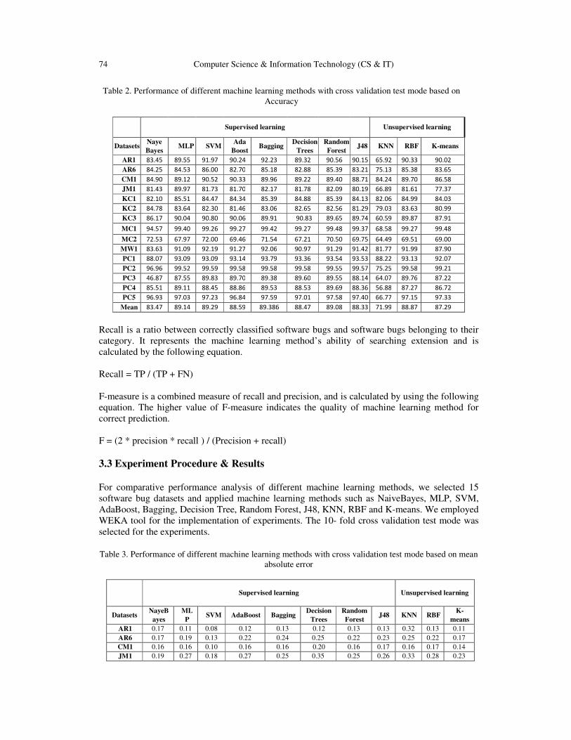
74 Computer Science & Information Technology (CS & IT)
Table 2. Performance of different machine learning methods with cross validation test mode based on
Accuracy
Supervised learning
Unsupervised learning
Datasets Naye
Bayes MLP SVM
Ada
Boost Bagging
Decision
Trees
Random
Forest J48 KNN RBF K-means
AR1 83.45 89.55 91.97 90.24 92.23 89.32 90.56 90.15 65.92 90.33 90.02
AR6 84.25 84.53 86.00 82.70 85.18 82.88 85.39 83.21 75.13 85.38 83.65
CM1 84.90 89.12 90.52 90.33 89.96 89.22 89.40 88.71 84.24 89.70 86.58
JM1 81.43 89.97 81.73 81.70 82.17 81.78 82.09 80.19 66.89 81.61 77.37
KC1 82.10 85.51 84.47 84.34 85.39 84.88 85.39 84.13 82.06 84.99 84.03
KC2 84.78 83.64 82.30 81.46 83.06 82.65 82.56 81.29 79.03 83.63 80.99
KC3 86.17 90.04 90.80 90.06 89.91 90.83 89.65 89.74 60.59 89.87 87.91
MC1 94.57 99.40 99.26 99.27 99.42 99.27 99.48 99.37 68.58 99.27 99.48
MC2 72.53 67.97 72.00 69.46 71.54 67.21 70.50 69.75 64.49 69.51 69.00
MW1 83.63 91.09 92.19 91.27 92.06 90.97 91.29 91.42 81.77 91.99 87.90
PC1 88.07 93.09 93.09 93.14 93.79 93.36 93.54 93.53 88.22 93.13 92.07
PC2 96.96 99.52 99.59 99.58 99.58 99.58 99.55 99.57 75.25 99.58 99.21
PC3 46.87 87.55 89.83 89.70 89.38 89.60 89.55 88.14 64.07 89.76 87.22
PC4 85.51 89.11 88.45 88.86 89.53 88.53 89.69 88.36 56.88 87.27 86.72
PC5 96.93 97.03 97.23 96.84 97.59 97.01 97.58 97.40 66.77 97.15 97.33
Mean 83.47 89.14 89.29 88.59 89.386 88.47 89.08 88.33 71.99 88.87 87.29
Recall is a ratio between correctly classified software bugs and software bugs belonging to their
category. It represents the machine learning method’s ability of searching extension and is
calculated by the following equation.
Recall = TP / (TP + FN)
F-measure is a combined measure of recall and precision, and is calculated by using the following
equation. The higher value of F-measure indicates the quality of machine learning method for
correct prediction.
F = (2 * precision * recall ) / (Precision + recall)
3.3 Experiment Procedure & Results
For comparative performance analysis of different machine learning methods, we selected 15
software bug datasets and applied machine learning methods such as NaiveBayes, MLP, SVM,
AdaBoost, Bagging, Decision Tree, Random Forest, J48, KNN, RBF and K-means. We employed
WEKA tool for the implementation of experiments. The 10- fold cross validation test mode was
selected for the experiments.
Table 3. Performance of different machine learning methods with cross validation test mode based on mean
absolute error
Supervised learning
Unsupervised learning
Datasets NayeB
ayes
ML
P SVM AdaBoost Bagging
Decision
Trees
Random
Forest J48 KNN RBF
K-
means
AR1 0.17 0.11 0.08 0.12 0.13 0.12 0.13 0.13 0.32 0.13 0.11
AR6 0.17 0.19 0.13 0.22 0.24 0.25 0.22 0.23 0.25 0.22 0.17
CM1 0.16 0.16 0.10 0.16 0.16 0.20 0.16 0.17 0.16 0.17 0.14
JM1 0.19 0.27 0.18 0.27 0.25 0.35 0.25 0.26 0.33 0.28 0.23

Computer Science & Information Technology (CS & IT) 75
KC1 0.18 0.21 0.15 0.22 0.20 0.29 0.19 0.20 0.18 0.23 0.17
KC2 0.16 0.22 0.17 0.22 0.22 0.29 0.22 0.23 0.21 0.23 0.21
KC3 0.15 0.12 0.09 0.14 0.14 0.17 0.14 0.13 0.39 0.15 0.12
MC1 0.06 0.01 0.01 0.01 0.01 0.03 0.01 0.01 0.31 0.01 0.01
MC2 0.27 0.32 0.28 0.39 0.37 0.40 0.35 0.32 0.35 0.41 0.31
MW1 0.16 0.11 0.08 0.12 0.12 0.15 0.12 0.12 0.18 0.12 0.13
PC1 0.11 0.11 0.07 0.11 0.10 0.14 0.09 0.10 0.12 0.12 0.08
PC2 0.03 0.01 0.00 0.01 0.01 0.02 0.01 0.01 0.18 0.01 0.01
PC3 0.51 0.14 0.10 0.16 0.15 0.21 0.15 0.15 0.36 0.18 0.13
PC4 0.14 0.12 0.11 0.15 0.14 0.16 0.14 0.12 0.43 0.20 0.13
PC5 0.04 0.03 0.03 0.04 0.03 0.06 0.03 0.03 0.33 0.05 0.03
Mean 0.16 0.14 0.10 0.15 0.15 0.18 0.14 0.14 0.27 0.16 0.13
Table 4. Performance of different machine learning methods with cross validation test mode based
on F-measure
Supervised learning Unsupervised learning
Datas
ets NayeBay
es MLP SVM AdaBoo st Bagging Decision
Trees Random Forest J48 KNN RBF K-
means AR1 0.90 0.94 0.96 0.95 0.96 0.94 0.96 0.95 0.79 0.95 0.94
AR6 0.90 0.91 0.93 0.90 0.92 0.90 0.92 0.90 0.84 0.92 0.90
CM1 0.91 0.94 0.95 0.95 0.95 0.94 0.94 0.94 0.91 0.95 0.93 JM1 0.89 0.90 0.90 0.90 0.90 0.90 0.90 0.88 0.80 0.90 0.86 KC1 0.90 0.92 0.92 0.91 0.92 0.92 0.92 0.91 0.89 0.92 0.91 KC2 0.90 0.90 0.90 0.88 0.90 0.89 0.89 0.88 0.86 0.90 0.88 KC3 0.91 0.94 0.95 0.95 0.95 0.95 0.94 0.94 0.72 0.95 0.93 MC1 0.97 1.00 1.00 1.00 1.00 1.00 1.00 1.00 0.81 1.00 1.00 MC2 0.82 0.78 0.82 0.80 0.81 0.77 0.80 0.78 0.76 0.81 0.77 MW1 0.90 0.95 0.96 0.95 0.96 0.95 0.95 0.95 0.89 0.96 0.93 PC1 0.94 0.97 0.96 0.96 0.97 0.97 0.97 0.97 0.94 0.96 0.96 PC2 0.99 1.00 1.00 1.00 1.00 1.00 1.00 1.00 0.90 1.00 1.00 PC3 0.60 0.94 0.95 0.95 0.94 0.95 0.94 0.94 0.77 0.95 0.93 PC4 0.92 0.94 0.94 0.94 0.94 0.93 0.94 0.93 0.72 0.93 0.92 PC5 0.98 0.99 0.99 0.98 0.99 0.98 0.99 0.99 0.80 0.99 0.99
Mean 0.89 0.93 0.942 0.93 0.94 0.93 0.93 0.93 0.82 0.93 0.92
i) The software bug repository datasets:
D= {AR1, AR6, CM1, JM1, KC1, KC2, KC3, MC1, MC2, MW1, PC1, PC2, PC3, PC4, PC5}
ii) Selected machine learning methods
M = {Nayes Bayes, MLP, SVM, AdaBoost, Bagging, Decision Tree, Random Forest, J48, KNN,
RBF, K-means}
Data pre-process:
a) Apply Replace missing values to D
b) Apply Discretize to D
Test Model - cross validation (10 folds): for each D do for each M do
Perform cross-validation using 10-folds
end for
Select accuracy
Select Mean Absolute Error (MAE) Select F-measure end for
Experiment procedure:
Input:

76 Computer Science & Information Technology (CS & IT)
Output: a) Accuracy
b) Mean Absolute Error
c) F-measure
3.4 Experiment results
Table 2, 3 & 4 show the results of the experiment. Three parameters were selected in order to
compare them such as Accuracy, Mean absolute error and F-measure. In order to compare the
selected algorithms the mean was taken for all datasets and the results are shown in Figure 1, 2 &
3.
Figure 1. Accuracy results for selected machine learning methods
Figure 2. MAE results for selected machine learning methods

Computer Science & Information Technology (CS & IT) 77
Figure 3. F-measure results for selected machine learning methods
4. DISCUSSION & CONCLUSION Accuracy, F-measure and MAE results are gathered on various datasets for different algorithms
as shown in Table 2, 3 & 4. The following observations were drawn from these experiment
results:
NaiveBayes classifier for software bug classification showed a mean accuracy of various datasets
83.47. It performed really well on datasets MC1, PC2 and PC5, where the accuracy results were
above 95%. The worst performance can be seen on dataset PC3, where the accuracy was less than
50%. MLP also performed well on MC1 and PC2 and got overall accuracy on various datasets
89.14 %. SVM and Bagging performed really well as compared to other machine learning
methods, and got overall accuracy of around 89 %. Adaboost got accuracy of 88.59, Bagging got
89.386, Decision trees achieved accuracy around 88.47, Random Forest got 89.08, J48 got 88.33
and in the case of unsupervised learning KNN achieved 71.99, RBF achieved 88.87 and K-means
achieved 87.29. MLP, SVM and Bagging performance on all the selected datasets was good as
compared to other machine learning methods. The lowest accuracy was achieved by KNN
method.
The best MAE achieved by SVM method which is 0.10 on various datasets and got 0.00 MAE for
PC2 dataset. The worst MAE was for KNN method which was 0.27. K-means, MLP, Random
Forest and J48 also got better MAE around 0.14. In the case of F-measure, higher is better.
Higher F-measure was achieved by SVM and Bagging methods which were around 0.94. The
worst F-measure as achieved by KNN method which was 0.82 on various datasets.
Software bugs identification at an earlier stage of software lifecycle helps in directing software
quality assurance measures and also improves the management process of software. Effective
bug’s prediction is totally dependent on a good prediction model. This study covered the different
machine learning methods that can be used for a bug’s prediction. The performance of different
algorithms on various software datasets was analysed. Mostly SVM, MLP and bagging
techniques performed well on bug’s datasets. In order to select the appropriate method for bug’s
prediction domain experts have to consider various factors such as the type of datasets, problem
domain, uncertainty in datasets or the nature of project. Multiple techniques can be combined in
order to get more accurate results.

78 Computer Science & Information Technology (CS & IT)
ACKNOWLEDGEMENT
The authors would like to thank Dr. Jagath Samarabandu for his constructive comments
which contributed to the improvement of this article as his course work.
REFERENCES [1] Kumaresh, Sakhti and Baskaran, R. (2010) “Defect analysis and prevention for software process
quality improvement”, International Journal of Computer Applications, Vol. 8, Issue 7, pp. 42-47.
[2] Ahmad, Khalil and Varshney, Natasha (2012)“On minimizing software defects during new product
development using enhanced preventive approach”, International Journal of Soft Computing and
Engineering, Vol. 2, Issue 5, pp. 9-12.
[3] Andersson, Carina (2007) “A replicated empirical study of a selection method for software reliability
growth models”, Empirical Software Engineering, Vol.12, Issue 2, pp. 161-182.
[4] Fenton, Norman E. & Ohlsson, Nichlas (2000) “Quantitative analysis of faults and failures in a
complex software system”, IEEE Transactions on Software Engineering, Vol. 26, Issue 8, pp. 797-
814.
[5] Khoshgoftaar, Taghi M. & Seliya, Naeem (2004) “Comparative assessment of software quality
classification techniques: An empirical case study”, Empirical Software Engineering, Vol. 9, Issue 3,
pp. 229-257.
[6] Khoshgoftaar, Taghi M., Seliya, Naeem & Sundaresh, Nandani (2006) “An empirical study of
predicting software faults with case-based reasoning”, Software Quality Journal, Vol. 14, Issue 2, pp.
85-111.
[7] Menzies, Tim., Greenwald, Jeremy & Frank, Art (2007) “Data mining static code attributes to learn
defect predictors”, IEEE Transaction Software Engineering., Vol. 33, Issue 1, pp. 2-13.
[8] Spiewak, Rick & McRitchie, Karen (2008) “Using software quality methods to reduce cost and
prevent defects”, Journal of Software Engineering and Technology, pp. 23-27.
[9] Shiwei, Deng (2009) “Defect prevention and detection of DSP-Software”, World Academy of
Science, Engineering and Technology, Vol. 3, Issue 10, pp. 406-409.
[10] Trivedi, Prakriti & Pachori, Som (2010) “Modelling and analyzing of software defect prevention
using ODC”, International Journal of Advanced Computer Science and Applications, Vol. 1, No. 3,
pp. 75- 77.
[11] Nair, T.R. Gopalakrishan & Suma, V. (2010) “The pattern of software defects spanning across size
complexity”, International Journal of Software Engineering, Vol. 3, Issue 2, pp. 53- 70.
[12] Lessmann, Stephen., Baesens, Bart., Mues, Christopher., & Pietsch, Swantje (2008) “Benchmarking
classification models for software defect prediction: A proposed framework and novel finding”, IEEE
Transaction on Software Engineering, Vol. 34, Issue 4, pp. 485-496.
[13] Sharma, Trilok C. & Jain, Manoj (2013) “WEKA approach for comparative study of classification
algorithm”, International Journal of Advanced Research in Computer and Communication
Engineering, Vol. 2, Issue 4, 7 pages.
[14] Kaur, Puneet Jai & Pallavi, (2013) “Data mining techniques for software defect prediction”,
International Journal of Software and Web Sciences (IJSWS), Vol. 3, Issue 1, pp. 54-57.
[15] Wang, Tao., Li, Weihua., Shi, Haobin., & Liu, Zun. (2011) “Software defect prediction based on
classifiers ensemble”, Journal of Information & Computational Science, Vol. 8, Issue 1, pp. 4241–
4254.
[16] Adiu, Surendra & Geethanjali, N. (2013) “Classification of defects in software using decision tree
algorithm”, International Journal of Engineering Science and Technology (IJEST), Vol. 5, Issue 6, pp.
1332-1340.
[17] Dommati, Sunil J., Agrawal, Ruchi., Reddy, Ram M. & Kamath, Sowmya (2012) “Bug classification:
Feature extraction and comparison of event model using Naïve Bayes approach”, International
Conference on Recent Trends in Computer and Information Engineering (ICRTCIE'2012), pp. 8-12.
[18] Xu Jie., Ho Danny. and Capretz Luiz Fernando (2010) "An empirical study on the procedure to derive
software quality estimation models", International Journal of Computer Science & Information
Technology (IJCSIT), AIRCC Digital Library, Vol. 2, Number 4, pp. 1-16.
Computer Science & Information Technology (CS & IT) 79
[19] G. Boetticher, Menzies, Tim & T. Ostrand, (2007) PROMISE Repository of Empirical Software
Engineering Data, http://promisedata.org/, West Virginia University, Department of Computer
Science.
[20] WEKA, http://www.cs.waikato.ac.nz/~ml/weka, accessed on December 13th, 2013.
AUTHORS
Saiqa Aleem received her MS in Computer Science (2004) from University of Central
Punjab, Pakistan and MS in Information Technology (2013) from UAEU, United Arab
Emirates. Currently, she is pursuing her PhD. in software engineering from University
of Western Ontario, Canada. She had many years of academic and industrial
experience holding various technical positions. She is Microsoft, CompTIA, and
CISCO certified professional with MCSE, MCDBA, A+ and CCNA certifications.
Dr. Luiz Fernando Capretz has vast experience in the software engineering field as
practitioner, manager and educator. Before joining the University of Western Ontario
(Canada), he worked at both technical and managerial levels, taught and did research
on the engineering of software in Brazil, Argentina, England, Japan and the United
Arab Emirates since 1981. He is currently a professor of Software Engineering and
Assistant Dean (IT and e-Learning), and former Director of the Software Engineering
Program at Western. He was the Director of Informatics and Coordinator of the
computer science program in two universities in Brazil. He has published over 200
academic papers on software engineering in leading international journals and conference proceedings, and
co-authored two books: Object-Oriented Software: Design an Maintenance published by World Scientific,
and Software Product Lines published by VDM-Verlag. His current research interests are software
engineering, human aspects of software engineering, software analytics, and software engineering
education. Dr. Capretz received his Ph.D. from the University of Newcastle upon Tyne (U.K.), M.Sc. from
the National Institute for Space Research (INPE-Brazil), and B.Sc. from UNICAMP (Brazil). He is a senior
member of IEEE, a distinguished member of the ACM, a MBTI Certified Practitioner, and a Certified
Professional Engineer in Canada (P.Eng.). He can be contacted at [email protected]; further information
can be found at: http://www.eng.uwo.ca/people/lcapretz/
Dr. Faheem Ahmed received his MS (2004) and Ph.D. (2006) in Software
Engineering from the Western University, London, Canada. Currently he is Associate
Professor and Chair at Thompson Rivers University, Canada. Ahmed had many years
of industrial experience holding various technical positions in software development
organizations. During his professional career he has been actively involved in the life
cycle of software development process including requirements management, system
analysis and design, software development, testing, delivery and maintenance. Ahmed
has authored and co-authored many peer-reviewed research articles in leading journals
and conference proceedings in the area of software engineering. He is a senior member of IEEE.

80 Computer Science & Information Technology (CS & IT)
INTENTIONAL BLANK

David C. Wyld et al. (Eds) : ITCS, CST, JSE, SIP, ARIA, DMS - 2015
pp. 81–87, 2015. © CS & IT-CSCP 2015 DOI : 10.5121/csit.2015.50109
ANALYSING ATTRITION IN OUTSOURCED
SOFTWARE PROJECT
Umesh Rao Hodeghatta1 and Ashwathanarayana Shastry
2
1Xavier Institute of Management, Bhubaneswar, India,
[email protected] 2i-Point Consulting Solutions, Bangalore, India
ABSTRACT
Information systems (IS) outsourcing has grown as a major business phenomenon, and widely
accepted as a business tool. Software outsourcing companies provide expertise, knowledge and
capabilities to their clients by taking up the projects both onsite and offsite. These companies
face numerous challenges including attrition of project members. Attrition is a major challenge
experienced by the outsourcing companies as it has severe impact on business, revenues and
profitability. In this paper, attrition data of a major software outsourcing company was
analysed and an attempt to find the reason for attrition is also made. The data analysis was
based on the data collected by an outsourcing company over a period of two years for a major
client. The results show that the client initiated attrition can have an impact on project and the
members quit the outsourcing company due to client initiated ramp down without revealing the
reason.
KEYWORDS
Software engineering, Project Management, Attrition, Software Outsourcing, Software Project.
1. INTRODUCTION
A successful software project can be attributed to rightly managing three critical factors – people,
process and technology [1] While the process and technology used largely influences the
schedule, the quality and the productivity of the project, the people factor directly impacts the
revenue and profitability of the project [2]. People leave the project for various reasons and every
project member leaving the project will result in ‘attrition’. As people develop skills and gain
knowledge when they work through the different life cycle stages of the project, the attrition in
the project will result in loss of skills and knowledge [3]. It takes a great deal of effort and time to
rebuild that skills and knowledge to ensure that the project keeps running smoothly. Hence many
project managers will maintain a small buffer of people who will pitch in whenever there is
attrition in the project so that the project schedule, quality and productivity will not get impacted.
However, the buffer of people will bring down the profitability of the project.
The attrition process in a software project is common and needs to be carefully managed [1]. In
large size projects (both in terms of the number of people and the duration), the attrition manifests
itself in two forms – one is the attrition initiated by the client due to budget constraints or non-
performance of employees, and the other is the attrition initiated by the project members
themselves either because they want to move out of the current project or they want to leave the
company he/she is working for. In either of the cases, it is important to understand the nature of
attrition and its impact on the project [4].

82 Computer Science & Information Technology (CS & IT)
The project schedule and quality of project work largely depends on the stability of the project
team members. If attrition in the project increases, there will be transference of knowledge from
the outgoing project member to the incoming project member. This will introduce a delay in the
project and if the transition is incomplete, the quality of the project work greatly suffers. Hence,
the attrition factor in outsourced software project should be carefully considered while planning
for a project.
The aim of this study is an attempt to understand whether there is any relationship between the
client initiated attrition and the project member initiated attrition. It is also an attempt to
understand whether the HR personnel are correctly capturing the reasons for any employee
quitting the company during the exit interview. A large outsourcing organization of India was
considered for the study from which a sample of 120 records over a period of 14 months was
analysed.
2. LITERATURE REVIEW According to Gopal et al. (2003), attrition largely impacts the profitability of a software project
and hugely depends on the nature of the project contract signed. A project with a fixed price
contract will impact the profitability due to higher attrition than a project with a time and material
contract. The role of a person in the project also impacts profitability. A project manager leaving
in the middle of a project with a fixed price contract will create more damage than a mere
project member leaving the project. In a project with time and material contract, key software
developers/leads can create more damage to the projects than the project manager himself.
According to Reel (1993) any of the key people leaving the project is a loss, as some of the
crucial knowledge that has been gained till then is lost. If the project analysts quit the project,
then the business requirement knowledge is lost. Similarly, if the project managers leave the
project, the project process knowledge is lost. If the programmers quit, the pace of development
will slow down. The best practices and lessons learnt during the project execution are largely held
with the project team members. Unless all the knowledge that is gained during project execution
is documented, this knowledge will be lost along with the people and takes a similar time period
to be re-built [7].
According to Sundararajan et al. (2013) IT skills are very critical to the success of software
projects. Companies spend a lot of money and time to build IT skills among its staff to prepare
them to deliver successful software projects. Investing in FTEs (Full Time Employees) will bring
stability to workforce and hence better quality of delivery. However, Jones (1994) highlights that
the higher rate of attrition higher the risks associated with a project. Some companies choose to
outsource a part of the project work to contractors or vendors. While outsourcing is one of the
strategies for mitigating the risk related to attrition, the outsourced work will not automatically
guarantee good quality of work. Accountability for the work done becomes a bigger issue to
handle in such situations.
Knowledge management (KM) is one of the key aspects of handling the continuity of business, in
wake of growing attrition in the software industry. It is one of the solutions to the problem arising
out of the staff attrition. It also helps in improving re-usability and hence the productivity of the
staff. Companies can also use KM to improve their profitability. But KM calls for huge
investments in infrastructure and a continuous push by the management to ensure that people
contribute to the KM repository [10].
Staffing decisions in software projects is quite complex and needs to go through a structured
process. Software projects will have to be delivered within budget, within schedule and with very
high quality [11]. Sharm et al. (2010) in their paper states that a staffing model should be defined

Computer Science & Information Technology (CS & IT) 83
for each type of software project and ‘what if’ scenarios should be analyzed to cover possible
risks due to staff attritions throughout the life cycle of the project. The most estimation models
consider staff allocation as one of the key ingredients to arrive at the right effort estimation and
hence the total cost of the project. Before the start of any project, the staff profile, their
experience levels, roles and productivity of each staff should be analyzed in detail to cover the
attrition risk in projects.
In their work by Lacity and Hirschheim (1993) have found that factors like cultural differences,
time zone differences, the quality of the staff, their knowledge retention and reuse impacting the
productivity of outsourced work. In fact, many organizations feel that they have not achieved the
real benefits of true outsourcing due to the above factors.
3. RESEACRH QUESTION All the above studies are based on small samples, single cases, specific industries and project
types, generalization might not be possible. In this study, ‘attrition’ is defined as any project
member leaving / quitting the client project. The reasons for leaving the project may be on
account of client initiation or by the project member’s desire to quit. The client can ask the
outsourcing company to reduce the project members in a team due to financial budget constraints
or non-performance of the team members. In such cases, the outsourcing company takes the
members out of the project and deploys the engineers in some other project. From the outsourcing
company perspective, this may not be considered as attrition. However, the company has to make
a decision whether to retain these members in the same project, without billing the client or
deploy them into other projects. This has an impact on the overall profitability of the project. In
other cases, the project members working at the client site quit the company altogether due to
better opportunities or some other reasons. This is considered as a true attrition for the
outsourcing company.
The objective of the research is to analyse the reasons for leaving a project, whether client
initiated or employee initiated, are similar in nature or not. In addition, an analysis is done on the
reasons given by the project members while quitting the company are same or different. Since
attrition in a large project can impact the revenues and profitability of the project, this analysis
helps companies in proper resource planning and retention.
Hypothesis 1 (H10): There is no difference between the sample mean of attrition caused due to
the client initiation and the project member initiation.
The objective was to statistically test the significance of attrition data. T-tests were performed to
confirm that the means of attrition in client initiated data were similar to the means of the attrition
in members initiated data.
Hypothesis 2 (H20): There is no difference between the sample mean of attrition of employees
joining another company and for personal reasons.
The objective was to statistically test the significance of attrition data. T-tests were performed to
confirm that the means of attrition in client initiated data were similar to means of the attrition of
members initiated data.
4. METHODOLOGY In this study, the attrition dataset from a major outsourcing company from India was analyzed.
The company is a global leader in consulting, technology, and outsourcing solutions. It has a

84 Computer Science & Information Technology (CS & IT)
client base with more than 250 clients across 30 countries and with an employee base of more
than 100000. For the study, the attrition data from one client was analysed. The outsourcing
company had deployed more than 300 engineers at the client’s site for a project. Whenever an
employee left the project, the reason for leaving was recorded and collated on a monthly basis. A
total of 120 records were available in the dataset. Out of the 120 records, after some data
cleaning, a total of 106 employee records were analysed. The data was collected over a period of
14 months. The project members who left the project were programmers, programmer analysts,
project managers, translators and UI designers. Every month, the attrition data was captured by
entering the pertinent information regarding the project member, including whether the member
was ramped down by the client, or the member had resigned from the outsourcing company. If
the member had resigned, then further data from the exit interview was also recorded. In this
dataset, only one reason was recorded – whether the exit was for personal reasons or for joining
another company. In this study, as per the outsourcing company norms, any member leaving the
project before 18 month is considered as attrition.
The descriptive data was analyzed using Statistical Package for Social Science (SPSS) Version
17, the statistical software package by IBM. SPSS is commonly used in the Social Science and in
the business world [14]. IBM SPSS allows in-depth data analysis and preparation, analytical
reporting, graphics and modelling (ibm.com). It is a Windows based program that can be used to
perform data analysis, create tables, graphs and statistical data analysis. It is capable of handling
large amounts of data and can perform visualization, ANOVA, t-test, Chi-square tests, F-test, and
other statistical analyses.
Further, in order to analyze the data at a micro level and test the difference between two groups at
a time, t-tests were conducted. The null hypothesis assumes that there is no significant difference
in the means of the two groups, in other words, the sample mean of attrition initiated either by the
client or the project members is the same.
5. RESULTS
The results of descriptive data on the study of attrition are important for the following reasons:
1). It enables a company to determine the compatibility of client initiated attrition and project
member initiated attrition. 2). It enables to determine the reasons for attrition by members are the
same or different.
The first part of the analysis is to identify whether the attrition of client initiation and project
members’ initiation are the same or different. The analysis was performed between two groups of
data – client initiated attrition and project members’ initiated attrition. The following Table 1
presents the descriptive data analysis:
Table 1. Attrition Statistics: Client and Members Initiated
Client Initiated Member Initiated
Mean 3.285714286 2.571428571
Standard Error 0.834875601 0.561730898
Median 2 1.5
Standard Deviation 3.123818458 2.101804562
Sample Variance 9.758241758 4.417582418
Peasron Coefficient 0.63 0.63
From the Table 1, it can be noted that the mean of client initiated is 3.25 persons per month with a
standard deviation of 3.12 whereas the members initiated is 2.57 persons per month with a

Computer Science & Information Technology (CS & IT) 85
standard deviation of 2.10 and both the groups are independent. Further, t-tests were conducted to
compare the behaviour between the two groups, whether they are same or different. Whether the
reasons for client initiated attrition and member initiated attrition are the same or they are
different. Further, correlation coefficient was found to be 0.63.
Table 2. T-test: Client and Members Initiated Attrition
Groups M SD t-value p-value
(two
tailed)
Null Hypothesis
Client
Initiated
3.28 3.12 1.099 0.29* Fail to Reject
Member
Initiated
2.57 2.10
*Significance level = 0.05
A paired-samples t-test was conducted to compare client initiated attrition and members initiated
attrition conditions. As shown in the Table 2, there was no significant difference in the scores for
client initiated (M=3.28, SD=3.12) and members initiated (M=2.57,SD=2.10) conditions with t-
value of 1.099 and p = 0.29. These suggest that there is not enough evidence to show that the
attrition due to client initiated and attrition due to members initiated are different.
The second part of the analysis is to identify the reasons given by the members who resign
(attrition) was to join the other company or some other reasons which is unknown. The analysis
was performed between the two sets of data – reasons joining the other company and reasons that
is unknown. The following Table 3 presents the descriptive data analysis:
Table 3. Attrition reasons: Joining other company and Unknown
Joining Other Company Unknown
Mean 0.92 1.64
Standard Error 0,304 0.487
Median 0.5 1
Standard Deviation 1.141 1.823
Sample Variance 1.302 3.324
From the Table 3, it can be noted that the mean of Joining Other Company is 0.92 persons per
month with a standard deviation of 1.14 whereas the Unknown is 1.64 persons per month with a
standard deviation of 1.82 and both the groups are independent. Further, t-tests, as shown in Table
4, were conducted to compare the behaviour between the two groups are same or different.
Whether reasons for Joining Other Company and Unknown are same or they are different.
Table 4: T-test: Joining Other Company and Unknown
Groups M SD t-value p-value
(two tailed)
Null Hypothesis
Joining
Other
Company
0.92 1.14 1.21 0.24 Fail to Reject
Unknown 1.64 1.82
*Significance level = 0.05

86 Computer Science & Information Technology (CS & IT)
A paired-samples t-test was conducted to compare Joining Other Company and Unknown
conditions. As shown in the Table 4, there was no significant difference in the scores for Joining
Other Company (M=0.92, SD=1.14) and Unknown (M=1.64,SD=1.82) conditions with t-value of
1.21 and p = 0.24. These suggest that there is not enough evidence to show that the reasons for
Joining Other Company and reasons for Unknown attrition by members initiated are different.
6. DISCUSSION The results indicate that there is no significant difference in the sample mean of client initiated
and members initiated attrition. It can be inferred from the results that the client initiated ramp
down can have significant impact on team members working on the project. Client initiated ramp
down can result in demotivating the team as the other team members do not feel secure about
their places in the project and hence not contribute to the best of their ability to the project and on
the personal side, not gain proper experience or skills which would help in their career. From the
results, it can be also inferred that the reasons given by the employees when they quit the
company is not properly captured. T-test shows that there is no significant difference in the
sample means of reasons for leaving the company.
Employees normally tend to quote ‘pursuing higher education’ as one of the main reasons for
members initiated attrition. The companies tend to go soft on this aspect and do not insist on
serving sufficient notice before reliving them from their duty. In other cases, employees quote
‘personal reasons’ which cannot be drilled down further as it would mean intruding in their
privacy. In case of client initiated attrition, some employees will treat it as an opportunity to move
on to new projects. But many employees will feel demotivated as their learning opportunity in
their current project got terminated due to ramp down in the account.
Hypothesis 1 (H10): There is no difference between the sample mean of attrition caused due to
the client initiation and the project member initiation.
Fail to reject as there is not enough evidence to show that the attrition due to client initiated and
attrition due to members initiated are different.
Hypothesis 2 (H20): There is no difference between the sample mean of attrition of employees
joining another company and for personal reasons.
Fail to reject as there is not enough evidence to show that the reasons for Joining Other Company
and reasons for Unknown attrition by members initiated are different.
6.1 Managerial Implications
From project management perspective, the impact of attrition on the project profitability will
remain the same irrespective of whether the attrition was initiated by the client or the project
member. The project manager will have to factor in the risk associated with the attrition on the
project output and accordingly handle his staffing plan to mitigate the risk. In case of client
initiated attrition, the project member has the option to come out of the current project and move
on to another project. Hence this attrition will not impact the attrition of the company. In case of
project member initiated attrition, both the project and the company will suffer and the cost of
mitigating the risk will be very high and hence will impact the profitability both the company and
its client.
Computer Science & Information Technology (CS & IT) 87
7. CONCLUSIONS
The study analyses the attrition in a project from an outsourcing company’s point of view and the
reasons behind the attrition. Further, the study shows that there is no significant difference
between the client initiated and members initiated attrition. Similarly, in the case of the members
initiated attrition, the reasons for leaving the company is not extensively captured by the company
and all these could have an impact on the overall project. The study was limited to only one client
because of data availability. This can be further extended to data from multiple clients and
multiple projects. Also in the next stage of the study, detail analysis of exit interview answers will
be analysed once there is a significant amount of data.
REFERENCES
[1] Ebert, C, (2012) “Global software and IT: a guide to distributed development, projects, and
outsourcing”, Wiley Publication, USA.
[2] Fink, Lior, (2014) “Why project size matters for contract choice in software development
outsourcing”, ACM SIGMIS Database, Vol. 45, No. 3.
[3] Narayanan Sriram, Balasubramanian Sridhar, and Swaminathan M. Jayashankar, (2010) “Managing
outsourced software projects: an analysis of project performance and customer satisfaction”,
Production and Operations Management, Vol. 20, No. 4, pp. 508–521.
[4] Lindnera Frank and Waldb Andreas, (2011) “Success factors of knowledge management in temporary
organizations”, International Journal of Project Management, Vol. 29, No. 7, pp. 877–888
[5] Gopal, A., Sivaramakrishnan, K., Krishnan, M. S., and Mukhopadhyay, T., (2003) “Contracts in
offshore software development: An empirical analysis”, Management Science, Vol. 49, No. 12, pp.
1671-1683.
[6] Reel, J. S., (1999, “Critical success factors in software projects”, Software, IEEE, Vol. 16, No. 3, pp.
18-23.
[7] Bradley S. J, Nguyen, N and Vidale, R.J, (1993) "Death of a software manager: how to avoid career
suicide through dynamic software process modeling", American Programmer, pp. 11-17.
[8] Sundararajan, S., Bhasi, M., and Pramod, K. (2013) “An empirical study of industry practices in
software development risk management”, International Journal of Scientific and Research
Publications, Vol. 3, No. 6.
[9] Jones, C., (1994) “Assessment and control of software risks“, Yourdon Press, Prentice Hall,
Englewood Cliffs, NJ.
[10] Anuradha Mathrani, David Parsons, Sanjay Mathrani, (2012) “Knowledge management initiatives in
offshore software development: vendors’ perspectives” Journal of Universal Computer Science, Vol.
18, No. 19, pp. 2706-2730
[11] Stefanie Betz, Andreas Oberweis and Rolf Stephan., (2014) “Knowledge transfer in offshore
outsourcing software development projects: an analysis of the challenges and solutions from German
clients”, Expert Systems, Vol. 31, No. 3, pp. 282–297
[12] Sharma, A., Sengupta, S., and Gupta, A., (2011) “Exploring risk dimensions in the Indian software
industry”, Project Management Journal, Vol. 42, No. 5, pp. 78-91.
[13] Lacity, M. C. and Hirschheim, R., (1993) “Information systems outsourcing: Myths, Metaphors and
Realities”, Wiley and Sons.
[14] Field, A., (2009) “Discovering statistics using SPSS”, Sage publications.
[15] www.ibm.com, last accessed Sept 2014.

88 Computer Science & Information Technology (CS & IT)
INTENTIONAL BLANK

David C. Wyld et al. (Eds) : ITCS, CST, JSE, SIP, ARIA, DMS - 2015
pp. 89–105, 2015. © CS & IT-CSCP 2015 DOI : 10.5121/csit.2015.50110
LSB STEGANOGRAPHY WITH IMPROVED
EMBEDDING EFFICIENCY AND
UNDETECTABILITY
Omed Khalind and Benjamin Aziz
School of Computing, University of Portsmouth, Portsmouth, United Kingdom
[email protected], [email protected]
ABSTRACT
In this paper, we propose a new method of non-adaptive LSB steganography in still images to
improve the embedding efficiency from 2 to 8/3 random bits per one embedding change even for
the embedding rate of 1 bit per pixel. The method takes 2-bits of the secret message at a time
and compares them to the LSBs of the two chosen pixel values for embedding, it always assumes
a single mismatch between the two and uses the second LSB of the first pixel value to hold the
index of the mismatch. It is shown that the proposed method outperforms the security of LSB
replacement, LSB matching, and LSB matching revisited by reducing the probability of
detection with their current targeted steganalysis methods. Other advantages of the proposed
method are reducing the overall bit-level changes to the cover image for the same amount of
embedded data and avoiding complex calculations. Finally, the new method results in little
additional distortion in the stego image, which could be tolerated.
KEYWORDS
Steganography, Embedding efficiency, Probability of detection, Single Mismatch, LSB
matching, LSB replacement
1. INTRODUCTION
Steganography is the art and the science of keeping the existence of messages secret rather than
only their contents, as it is the case with cryptography. Both steganography and digital
watermarking belong to information hiding, but they differ in their purpose. Digital watermarking
is intended to protect the cover, whereas steganography is used to protect the message. So,
steganography is considered broken when the existence of the secret message is detected. Hence,
the most important property for every steganographic method is undetectability by the existing
steganalysis techniques.
LSB steganography is the most widely used embedding method in pixel domain, since it is easy
to implement, has reasonable capacity, and is visually imperceptible. Unfortunately, both methods
of LSB steganography (LSB replacement and LSB matching) are detectable by the current
steganalysis approaches discussed in later sections.
There are some methods proposed to improve the capacity of LSB replacement like[1,2], or to
avoid changing the histogram of the cover image like [3] which reduce the embedding capacity
by 50%. As mentioned earlier, the undetectability, or the probability of detection is the most
important property for any steganographic method. In this paper a new method of non-adaptive

90 Computer Science & Information Technology (CS & IT)
LSB steganography is proposed to reduce the probability of detection for the same amount of data
embedded with LSB replacement, LSB matching, and LSB matching revisited [4]by the current
detection methods. The proposed method also results in fewer ENMPP (Expected Number of
Modifications Per Pixel) in both pixel and bit-level to the cover image, and changes the histogram
of the cover image in a different way without any complex calculation.
The paper is organized like the following; it starts with clarifying adaptive and non-adaptive
steganography and the related embedding methods in the literature. Then, it starts analysing both
LSB replacement and LSB matching in grey-scale images from different perspectives such as the
embedding efficiency, histogram changes, and bit-level ENMPP. Then, the proposed method is
explained and followed by the same analysis process. After that, the experimental results are
shown for the proposed method against both steganalysis methods; LSB replacement and LSB
matching. Finally, the conclusion and future work are discussed in the last section.
2. ADAPTIVE AND NON-ADAPTIVE LSB STEGANOGRAPHY IN IMAGE
The embedding process of LSB steganography relies on some methods for selecting the location
of the change. In general, there are three selection rules to follow in order to control the location
of change, which are either sequential, random, or adaptive [5].
A sequential selection rule modifies the cover object elements individually by embedding the
secret message bits in a sequential way. For example, it is possible to embed the secret message
by starting from the top-left corner of an image to the bottom-right corner in a row-wise manner.
This selection rule, sequential, is very easy to implement, but has a very low security against
detection methods.
A pseudo-random selection rule modifies the cover object by embedding the secret message bits
into a pseudo randomly chosen subset of the cover object, possibly by using a secret key as a
pseudo-random number generator (PRNG). This type of selection rule gives a higher level of
security than sequential methods.
An adaptive selection rule modifies the cover object by embedding the secret message bits in
selected locations based on the characteristics of the cover object. For example, choosing noisy
and high textured areas of the image, which are less detectable than smooth areas for hiding data.
This selection rule, adaptive, gives a higher security than sequential and pseudo-random selection
rules in terms of detection.
So, the non-adaptive image steganography techniques are modifying the cover image for message
embedding without considering its features (content). For example LSB replacement and LSB
matching with sequential or random selection of pixels are modifying the cover image according
to the secret message and the key of random selection of pixels without taking the cover image
properties into account. Whereas, adaptive image steganography techniques are modify the cover
image in correlation with its features [6]. In other words, the selection of pixel positions for
embedding is adaptive depending on the content of the cover image. The bit-plane complexity
segmentation (BPCS) proposed by Kawguchi[7] is an early typical method of adaptive
steganography.
As adaptive steganographic schemes embed data in specific regions (such as edges), the
steganographic capacity of such method is highly depend on the cover image used for embedding.
Therefore, in general it is expected to have less embedding rate than non-adaptive schemes.
However, steganographers have to pay this price in order to have a better security or less
detectable stego image.

Computer Science & Information Technology (CS & IT) 91
3. RELATED WORKS
The undetectability is the most important requirement of any steganographic scheme, which is
affected by the choice of the cover object, the type of embedding method, the selection rule of
modifying places, and the number of embedding changes which is directly related to the length of
secret message[8].
If two different embedding methods share the same source of cover objects, the same selection
method of embedding place, and the same embedding operation, the one with less number of
embedding changes will be more secure (less detectable). This is because the statistical property
of the cover object is less likely to be disrupted by smaller number of embedding changes[8].
The concept of embedding efficiency is introduced by westfeld[9], and then considered as an
important feature of steganographic schemes[10,11], which is the expected number of embedded
random message bits per single embedding change[12].
Reducing the expected number of modifications per pixel (ENMPP) is well studied in the
literature considering the embedding rate of less than 1 , like westfeld’s F5-algorithm[13], which
could increase the embedding efficiency only for short messages. However, short messages are
already challenging to detect. Also, the source coding-based steganography (matrix embedding)
proposed by Fridrich et al.[8,12], which are extensions of F5-algorithm improved the embedding
efficiency for large payloads but still with embedding rate of less than 1. The stochastic
modulation proposed by Fridrich and Goljan[14], is another method of improving the security for
the embedding rate of up to 0.8 bits/ pixel.
For the embedding rate of 1, there have been some methods for improving the embedding
efficiency of LSB matching like Mielikainen[4], which reduced the ENMPP with the same
message length from 0.5 to 0.375. The choice of whether to add or subtract one to/from a pixel
value of their method relies on both the original pixel values and a pair of two consecutive secret
bits. However, this method of embedding cannot be applied on saturated pixels (i.e. pixels with
values 0 and 255), which is one of the drawbacks of this method. Then, the generalization method
of LSB matching is proposed by Li et al.[15] with the same ENMPP for the same embedding rate
using sum and difference covering set (SDCS). Another method of improving the embedding
efficiency of LSB matching is proposed by Zhang et al.[16], using a combination of binary codes
and wet paper codes, The embedding efficiency of this method can achieve the upper bound of
the generalized ±1 embedding schemes.
However, no method could be found in the literature to improve the embedding efficiency of non-
adaptive LSB replacement, which is 2 bits per embedding change, for the embedding rate of 1.
So, developing such a method could be more useful than other adaptive methods in reusability
perspective. Moreover, the non-adaptive LSB embedding methods with higher embedding
efficiency can be used by existing adapted embedding methods to improve the steganographic
capacity and reduce the probability of detection. A good example is the LSB matching
revisited[4], which has been extended by[17,19].
Also, moving from non-adaptive to adaptive LSB embedding method does not mean that
improving the non-adaptive methods are impossible or useless, as we mentioned earlier, the LSB
matching revisited[4] is a very good example to support this fact.
4. ANALYSIS OF LSB REPLACEMENT
In this section, LSB replacement is analysed in three perspectives; the embedding process itself
(with its embedding efficiency), its effect on the intensity histogram after embedding process, and

92 Computer Science & Information Technology (CS & IT)
the bit-level ENMPP for each bit of the secret message. Also, the main weaknesses of this
embedding method are highlighted with the steganalysis methods that can detect it.
LSB replacement steganography simply replaces the LSB of the cover image pixel value with the
value of a single bit of the secret message. It leaves the pixel values unchanged when their LSB
value matches the bit value of the secret message and changes the mismatched LSB by either
incrementing or decrementing the even or odd pixel values by one respectively[4], as shown in
Figure 1.
Figure1. Possible pixel value transitions with LSB replacement
The embedding algorithm of the LSB replacement can be formally described as follows:
�� = ��� + 1 , � � ≠ ������� ��� �� � ������ − 1 , � � ≠ ������� ��� �� � ����� , � � = ������� �
To analyse the influence of the LSB replacement on the cover image intensity histogram, we
should consider that there is a probability of 50% for the LSB of the cover image pixel value to
already have the desired bit value. Therefore, the probability of modified pixel values will be
(P/2) for an embedding rate of P and the unmodified pixel values will be (1-P/2) after embedding
process, which means that embedding each message bit needs 0.5 pixel values to be changed. In
other words, it has an embedding efficiency of 2 bits of the secret message per one embedding
change. Hence, the intensity histogram of the stego image could be estimated as follows: h��n� = �1 − P2" h#�n� + P2 $h#�n + 1� , n is evenh#�n − 1� , n is odd �
Where n is a greyscale level which ranges from 0 to 255, and h�n� indicates the number of pixels
in the image with greyscale value of n.
This type of embedding, LSB replacement, leads to an imbalance distortion and produces ‘Pairs
of Values’ on the intensity histogram of the stego image. Since LSB replacement is inherently
asymmetric, current steganalysis methods can detect it easily[20], like: RS[21], SP[22], and
WS[23,24].
Another way of analysing LSB embedding is the bit-level ENMPP, which is the expected number
of bit modifications per pixel. This would be important too, as there are some steganalysis
methods that can detect the existence of the secret message based on calculating several binary
similarity measures between the 7th and 8th bit planes like[25]. Hence, an embedding process with
less bit-level ENMPP would be better and less detectable by such detection methods.

Computer Science & Information Technology (CS & IT) 93
The overall bit-level ENMPP for LSB replacement could be estimated by multiplying the
probability of having mismatched LSBs, P+�M�, which is 0.5 by the number of bits that needs to
be changed in each case, as shown below.
bit − level ENMPP = P+2M3 × no. of modi8ied bits bit − level ENMPP = 0.5 × 1 = 0.5 bits per message bits
Hence, the overall bit-level ENMPP for LSB replacement is 0.5 bits for each bit of the secret
message.
5. ANALYSIS OF LSB MATCHING
To analyse LSB matching steganography, we again consider the embedding process (with its
embedding efficiency), its effect on the intensity histogram of the cover image, and bit-level
ENMPP.
LSB matching or ±1 embedding is a modified version of LSB replacement. Instead of simply
replacing the LSB of the cover image, it randomly either adds or subtracts 1 from the cover image
pixel value that has mismatched LSB with the secret message bit[26]. The possible pixel value
transitions of ±1 embedding are shown in Figure 2.
Figure 2. Possible pixel value transitions with LSB matching
The random increment or decrement in pixel values should maintain the boundary limitation and
pixel values should always be between 0 and 255 [27]. In other words, the embedding process
should neither subtract 1 from pixel values of 0 nor add 1 to the pixel values of 255.
This random ±1 change to the mismatched LSB pixel values avoids the asymmetry changes to the
cover image, which is the case with LSB replacement. Hence, LSB matching is considered harder
to detect than LSB replacement[4]. The embedding procedure of LSB matching can be formally
represented as follows[28]:
P� = �P# + 1 , if b ≠ LSB(P#) and (K > 0 �D P# = 0) P# − 1 , if b ≠ LSB(P#) and (K < 0 �D P# = 255)P# , if b = LSB(P#) �
Where K is an independent and identically distributed random variable with uniform distribution
on F−1, +1G.

94 Computer Science & Information Technology (CS & IT)
For the intensity histogram we consider an embedding rate of P. There is a chance of 50% that the
clean image pixel value contains the desired LSB, which means that (P/2) of the cover pixel
values will change after the embedding process. Hence, the estimated unmodified pixel values
will be (1 − P/2) , which means that embedding each message bit needs 0.5 pixel values to be
changed. In other words, its embedding efficiency is 2 bits of the secret message per one
embedding change. The intensity histogram of the stego image could be obtained as follows[28].
h�(n) = �1 − P2" h#(n) + P4 Jh#(n + 1) + h#(n − 1)K
As mentioned earlier, the LSB matching will avoid the asymmetric property in modifying the
cover image. However, as claimed by[29], ±1 embedding is reduced to a low pass filtering of the
intensity histogram. This implies that the cover histogram contains more high-frequency power
than the histogram of the stego image [28], which offers an opportunity to steganalyzers to detect
the existence of the secret message embedded with LSB matching.
Apart from the supervised machine learning detectors of ±1 embedding like[30-33], which
usually have problems in choosing an appropriate feature set and measuring classification error
probabilities[34], the methods of detecting LSB matching steganography could be divided into
two categories; the centre of mass of the histogram characteristic function (HCF) and the
amplitude of local extrema (ALE)[35].
A number of detection methods have been proposed based on the centre of mass of the histogram
characteristic function (HCF-COM) like Harmsen and Pearlman[36], which has better
performance on RGB images than grey-scale. This method is modified and improved by Ker[27],
who applied the HCF in two novel ways: using the down sampled image and computing the
adjacency histogram.
Based on the amplitude of local extrema (ALE), Zhang et al.[29] considered the sum of the
amplitudes of all local extrema in the histogram to distinguish between stego and clean images.
This method is improved by Cancelli et al. [32] after reducing the border effects noise in the
histogram and extending it to the amplitude of local extrema in the 2D adjacency histogram.
The bit-level ENMPP of LSB matching is also important and should be considered for the same
reason, binary similarity measures. Since the probability of having mismatched LSB is also 50%,
the bit-level ENMPP would be as follows:
bit − level ENMPP = P+2M3 × no. of modi8ied bits bit − level ENMPP = 0.5 × (≥ 1) bit − level ENMPP ≥ 0.5 (bits per message bits)
Where P+ is the probability of having mismatched LSBs, which is 0.5. However, the number of
modified bits would be more than 1, because of the random ±1 changes to the pixel values, as
could be noted from the following examples:
127 (0111111)2 + 1 = 128 (10000000)2 , 8-bits changed
192 (11000000)2 - 1 = 191 (10111111)2 , 7-bits changed
7 (00000111)2 + 1 = 8 (00001000)2 , 4-bits changed
240 (11110000)2 - 1 = 239 (11101111)2 , 5-bits changed
Hence, the overall bit-level ENMPP for LSB matching is expected to be more than or equal to 0.5
bits for each bit of the secret message.

Computer Science & Information Technology (CS & IT) 95
6. THE PROPOSED METHOD
Based on highlighting the weakest part of both LSB replacement and ±1 embedding, in this
section we propose a new method of LSB embedding to improve the embedding efficiency and
reduce the probability of detection by current steganalysis methods. Moreover, the new proposed
method should also minimize the bit-level ENMPP to the cover image after embedding.
The new method, single mismatch LSB embedding (SMLSB), takes two bits of the secret
message at a time and embeds them in a pair of selected pixel values of the cover image. The
embedding method always assumes a single mismatch between the 2-bits of the secret message
and the LSBs of the selected pair of pixel values. For each 2-bits of the secret message we
consider two consecutive pixel values for simplicity. However, the selection could be based on
other functions as well.
Since the proposed method embeds 2-bits at a time, there are four cases of having match (M) or
mismatch (M) between the LSBs of the selected two pixel values and the 2-bits of the secret
message, as shown in Figure 3.
Figure 3. The possible cases of Match/ Mismatch
As the embedding method always assumes a single mismatch (MM or MM) between pixel values
and secret message bits, the 2nd
LSB of the first pixel value should always refer to the index of the
mismatch; 1 for MM and 0 for MM. If the case is MM, then it changes one of the LSBs according
to 2nd LSB of the first pixel value. If the 2nd LSB value was 0, then it flips the LSB of the first
pixel value to create MM. Otherwise, if it was 1, it flips the LSB of the second pixel value to
create MM. For the MM case, the embedding will also change one of the LSBs according to 2nd
LSB of the first pixel value. But this time, if the 2nd LSB was 0, then it flips the LSB of the
second pixel value to create MM. Otherwise, if it was 1, it flips the LSB of the first pixel value to
create MM.
For the other two cases, MM and MM, the embedding will be done by changing the 2nd
LSB of the
first pixel value based on the index of the mismatch. If it was MM, then the 2nd LSB of the first
pixel value will be set to 1. Otherwise, if it was MM, then the 2nd LSB value of the first pixel
value will be set to 0. Hence, after each embedding there is only MM or MM with the right index
in the 2nd LSB of the first pixel value. The embedding algorithm is shown in Figure .

96 Computer Science & Information Technology (CS & IT)
Figure 4. The embedding algorithm of SMLSB embedding
Table 1, shows some examples of the embedding process by the proposed method.
Table 1. Examples of SMLSB embedding process.
Clean pair of pixels Two message bits Stego pair of pixels
xxxxxx01
xxxxxxx1 11
xxxxxx00
xxxxxxx1
xxxxxx11
xxxxxxx0 10
xxxxxx11
xxxxxxx1
xxxxxx01
xxxxxxx1 00
xxxxxx01
xxxxxxx0
xxxxxx11
xxxxxxx0 01
xxxxxx10
xxxxxxx0
xxxxxx11
xxxxxxx0 11
xxxxxx11
xxxxxxx0
xxxxxx01
xxxxxxx1 10
xxxxxx11
xxxxxxx1
xxxxxx11
xxxxxxx0 01
xxxxxx01
xxxxxxx0
xxxxxx00
xxxxxxx0 10
xxxxxx00
xxxxxxx0
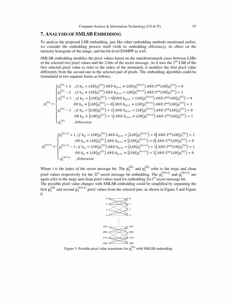
Computer Science & Information Technology (CS & IT) 97
7. ANALYSIS OF SMLSB EMBEDDING
To analyse the proposed LSB embedding, just like other embedding methods mentioned earlier,
we consider the embedding process itself (with its embedding efficiency), its effect on the
intensity histogram of the image, and the bit-level ENMPP as well.
SMLSB embedding modifies the pixel values based on the match/mismatch cases between LSBs
of the selected two pixel values and the 2-bits of the secret message. As it uses the 2nd LSB of the
first selected pixel value to refer to the index of the mismatch, it modifies the first pixel value
differently from the second one in the selected pair of pixels. The embedding algorithm could be
formulated in two separate forms as follows.
M��NO� =
PQQQRQQQSM��NO� + 2 , � �NO = ���2M��NO�3 TUV �NOWX ≠ ���2M��NOWX�3 TUV 2YZ���2M��NO�3 = 0 M��NO� − 2 , � �NO ≠ ���2M��NO�3 TUV �NOWX = ���2M��NOWX�3 TUV 2YZ���2M��NO�3 = 1 M��NO� + 1 , � �NO = [���2M��NO�3 = 0\TUV �NOWX = ���2M��NOWX�3 TUV 2YZ���2M��NO�3 = 0 ]^ �NO ≠ [���2M��NO�3 = 0\ TUV �NOWX ≠ ���2M��NOWX�3 TUV 2YZ���2M��NO�3 = 1M��NO� − 1 , � �NO = [���2M��NO�3 = 1\ TUV �NOWX = ���2M��NOWX�3 TUV 2YZ���2M��NO�3 = 0 ]^ �NO ≠ [���2M��NO�3 = 1\ TUV �NOWX ≠ ���2M��NOWX�3 TUV 2YZ���2M��NO�3 = 1M��NO� , ]_ℎ�Da��
�
M��NOWX� =PQQRQQSM��NOWX� + 1 , � �NO = ���2M��NO�3 TUV �NOWX = [���2M��NOWX�3 = 0\ TUV 2YZ���2M��NO�3 = 1 ]^ �NO ≠ ���2M��NO�3 TUV �NOWX ≠ [���2M��NOWX�3 = 0\ TUV 2YZ���2M��NO�3 = 0M��NOWX� − 1 , � �NO = ���2M��NO�3 TUV �NOWX = [���2M��NOWX�3 = 1\ TUV 2YZ���2M��NO�3 = 1 ]^ �NO ≠ ���2M��NO�3 TUV �NOWX ≠ [���2M��NOWX�3 = 1\ TUV 2YZ���2M��NO�3 = 0M��NOWX� , ]_ℎ�Da��
�
Where i is the index of the secret message bit. The p��Nb� and p#�Nb�
refer to the stego and clean
pixel values respectively for the 2ith secret message bit embedding. The p��NbWX� and p#�NbWX�
are
again refer to the stego and clean pixel values used for embedding 2i+1th secret message bit.
The possible pixel value changes with SMLSB embedding could be simplified by separating the
first p��Nb� and second p��NbWX�
pixel values from the selected pair, as shown in Figure 5 and Figure
6.
Figure 5. Possible pixel value transitions for p��Nb�
with SMLSB embedding

98 Computer Science & Information Technology (CS & IT)
Figure 6. Possible pixel value transitions for p��NbWX�
with SMLSB embedding
As could be noted from Figure and Figure , the pixel value transitions of p��NbWX� are like LSB
replacement. While p��Nb� is more complicated and has more transitions between clean and stego
pixel values.
To analyse the impact of the SMLSB embedding on the intensity histogram, again we consider an
embedding rate of P. Since the secret message is considered as a random sequence of 0 and 1,
based on the fact that it will be close to its encrypted version [37], equal probabilities should be
considered for match/mismatch cases. Hence, for each case of (MM, MM, MM, MM) the
probability of occurrence would be 0.25.
For MM and MM, the embedding process will change one of the two selected pixel values
according to the 2nd
LSB of the p#�Nb� to get either MM or MM. The change will be -1 or +1 for the
odd and the even pixel values respectively. So, (P/4) of the pixel values will be modified by
adding or subtracting 1 according to their values, even or odd values respectively.
However, for MM and MM there is a probability of having 50% of the 2nd
LSB of the p#�Nb� to have
the desired value, which needs no change. The other 50% will be modified by flipping the 2nd
LSB of the p#�Nb� only. In other word (P/8) of the pixel values will either incremented or
decremented by 2 according to their 2nd
LSB value. Hence, the remaining �1 − 3P/8� pixel
values will stay unchanged after embedding the secret message with the embedding rate of P,
which means that embedding each message bit needs 0.375 pixel values to be changed. This
ENMPP, 0.375, is better than LSB replacement and LSB matching, which are 0.5 pixels per
message bit. Hence, it improves the embedding efficiency from 2 to 8/3 bits per embedding
change. The intensity histogram of the stego image could be estimated by the following:
h��n� = �1 − 3P8 " h#�n� + P8 eh#�n + 2� , if 2fg LSB�n� = 0h#�n − 2� , if 2fg LSB�n� = 1� + P4 $h#�n + 1� , n is evenh#�n − 1� , n is odd �
Where, n is again the greys-cale level valued between 0 and 255. Both h��n� and h#�n� refer to
the number of pixels in the stego and clean image respectively with the greyscale value of n.
As only (P/4) of the pixel values are modified like LSB replacement, it is expected to effectively
reduce the probability of detection with LSB replacement steganalysis methods. Also, it is
expected to reduce the probability of detection by LSB matching steganalysis methods as well,
based on the dissimilarity in pixel value transitions and its influence on the intensity histogram
after embedding.

Computer Science & Information Technology (CS & IT) 99
The bit-level ENMPP for the proposed method could be calculated based on the match/mismatch
cases, in which equal probabilities are considered.
bit − level ENMPP = ∑�P+[each case] × no. of modi8ied bits�2
bit − level ENMPP = P+�MM� × 1 + P+2MM3 × 0.5 + P+2MM3 × 0.5 + P+2MM3 × 12
bit − level ENMPP = 0.25 × 1 + 0.25 × 0.5 + 0.25 × 0.5 + 0.25 × 12
bit − level ENMPP = 0.752 = 0.375 bits per message bit
The bit-level ENMPP is divided by two, as it embeds two bits of the secret message at a time. In
this case the overall bit-level ENMPP for the proposed method will be 0.375 bits per message bit.
Hence, the proposed method will result in fewer bit-level changes to the cover image after
embedding the same amount of secret message.
8. EXPERIMENTAL RESULTS
To make the experimental results more reliable, two sets of images are considered. The first set is
3000 images from ASIRRA (Animal Species Image Recognition for Restricting Access) public
corpus pet images from Microsoft research website[38], which are random with different sizes,
compression rates, texture ...etc. The other group is a set of 3000 never compressed images from
Sam Houston state university – Multimedia Forensics Group image database [39]. Both sets are
used after converting them into grey-scale images.
To check the efficiency of the proposed LSB embedding, both detection methods are considered;
the LSB replacement and LSB matching steganalysis methods. In all experiments, streams of
pseudo random bits are considered as a secret message. This is due to the fact that it will have all
statistical properties of encrypted version of the secret message according to[40]. Also, to
eliminate the effect of choosing the embedding place (random or sequential embedding), the
embedding rate of 1 bit per pixel (i.e. the images’ total capacity) is considered. Then it is tested
against both LSB replacement and matching steganalysis methods as shown in the following
sections.
8.1 SMLSB against LSB replacement steganalysis methods
There are many methods for detecting LSB replacement steganography in the literature, this
paper considers two structural steganalysis methods, the Sample Pair (SP) analysis[41] and
Weighted Stego (WS)[24]. As mentioned earlier, for each case, the image is loaded with the
maximum capacity of the random secret message twice; one with LSB replacement and the other
with SMLSB embedding.
The experimental results showed that the proposed method effectively reduce the probability of
detection for both detection methods over both sets of images compared to LSB replacement, as
shown in Table 2.

100 Computer Science & Information Techno
Table 2. The o
Image set
ASIRRA
Uncompressed
ASIRRA
Uncompressed
Also, there is a noticeable reduction in
the LSB replacement by SMLSB embedding as shown in
Figure 7. The probability of detection vs. detection threshold for ASIRRA images with WS.
Figure 8. The probability of detection vs. detection threshold for uncompressed images with WS.
Figure 9. The probability of detection vs. detection threshold for ASIRRA images with SP.
Computer Science & Information Technology (CS & IT)
overall reduction rates in probability of detection.
Detection method The overall reduction in
probability of detection
WS 46.5%
WS 48.4%
SP 30.9%
SP 39.8%
Also, there is a noticeable reduction in probability of detection for the threshold values that suits
the LSB replacement by SMLSB embedding as shown in Figures 7-10.
The probability of detection vs. detection threshold for ASIRRA images with WS.
The probability of detection vs. detection threshold for uncompressed images with WS.
The probability of detection vs. detection threshold for ASIRRA images with SP.
for the threshold values that suits
The probability of detection vs. detection threshold for ASIRRA images with WS.
The probability of detection vs. detection threshold for uncompressed images with WS.
The probability of detection vs. detection threshold for ASIRRA images with SP.

Computer Science & Information Technology (CS & IT)
Figure 10. The probability of detection vs. detection threshold for uncompressed images with SP.
8.2 SMLSB against LSB matching steganalysis m
As mentioned earlier, there are two main categories of LSB matching steganalysis methods. In
this paper we use one detection method in each category. For the centre of mass of the histogram
characteristic function (HCF-COM) we used Ker’s method in
extrema we used the method proposed by Zhang et al.
The proposed method, SMLSB, o
embedding methods in terms of detection. Figures 11
images with two different detection methods.
ALE based steganalysis method is no more than a random classifier for the stego images
embedded with SMLSB. Also, the performance of the HCF
considerably reduced by applying the SMLSB embedding method, as shown in Figures 13 and
14.
Figure 11. ROC graph of ALE steganalysis for LSB matching, LSB matching revisited
Computer Science & Information Technology (CS & IT)
The probability of detection vs. detection threshold for uncompressed images with SP.
matching steganalysis methods
As mentioned earlier, there are two main categories of LSB matching steganalysis methods. In
detection method in each category. For the centre of mass of the histogram
COM) we used Ker’s method in[27], and for the amplitude of local
extrema we used the method proposed by Zhang et al.[29].
The proposed method, SMLSB, outperforms both LSB matching and LSB matching revisited
embedding methods in terms of detection. Figures 11-14, show the ROC graph for each group of
images with two different detection methods. As could be noticed from Figures 11 and 12, the
steganalysis method is no more than a random classifier for the stego images
embedded with SMLSB. Also, the performance of the HCF-COM based steganalysis method is
considerably reduced by applying the SMLSB embedding method, as shown in Figures 13 and
ROC graph of ALE steganalysis for LSB matching, LSB matching revisited, and
ASIRRA images.
101
The probability of detection vs. detection threshold for uncompressed images with SP.
As mentioned earlier, there are two main categories of LSB matching steganalysis methods. In
detection method in each category. For the centre of mass of the histogram
, and for the amplitude of local
utperforms both LSB matching and LSB matching revisited [4]
14, show the ROC graph for each group of
As could be noticed from Figures 11 and 12, the
steganalysis method is no more than a random classifier for the stego images
COM based steganalysis method is
considerably reduced by applying the SMLSB embedding method, as shown in Figures 13 and
, and SMLSB for

102 Computer Science & Information Techno
Figure 12. ROC graph of ALE steganalysis for LSB matching, LSB matching revisited
Figure 13. ROC graph of HCF-COM steganalysis for LSB matching, LSB matching revisited
Figure 14. ROC graph of HCF-COM steganalysis for LSB matching, LSB matching revisited
Like any other steganography methods, the SMLSB cannot avoid all limitations and cannot
totally defeat the detection methods. As could be noticed from
possible to entirely avoid the detection. Also, there is another weak
quality measurement PSNR (Peak Signal to Noise Ratio)
The proposed method results in a slightl
LSB matching and LSB matching revisited
lower limit value of PSNR (38 dB)
Computer Science & Information Technology (CS & IT)
ROC graph of ALE steganalysis for LSB matching, LSB matching revisited, and
Uncompressed images.
COM steganalysis for LSB matching, LSB matching revisited
for ASIRRA images.
COM steganalysis for LSB matching, LSB matching revisited
for Uncompressed images.
Like any other steganography methods, the SMLSB cannot avoid all limitations and cannot
totally defeat the detection methods. As could be noticed from Table 2 and Figures 7
possible to entirely avoid the detection. Also, there is another weakness regarding
quality measurement PSNR (Peak Signal to Noise Ratio) between the cover and a stego image.
The proposed method results in a slightly lower PSNR than other methods; LSB replacement,
and LSB matching revisited, which is imperceptible and still very far from the
dB) according to [42, 43].
, and SMLSB for
COM steganalysis for LSB matching, LSB matching revisited, and SMLSB
COM steganalysis for LSB matching, LSB matching revisited, and SMLSB
Like any other steganography methods, the SMLSB cannot avoid all limitations and cannot
Figures 7-14, it is not
ness regarding the image
between the cover and a stego image.
LSB replacement,
very far from the

Computer Science & Information Technology (CS & IT) 103
Table 3 shows the PSNR values for some standard images after embedding random binary
streams with a maximum capacity using different embedding methods.
Table 13. PSNR values vs. embedding methods.
Images LSB Replacement LSB Matching LSB Matching
Revisited
SMLS
B
Lena 50.88 50.88 52.13 49.12
Pepper 50.17 50.17 51.41 48.42
Baboon 50.28 50.28 51.53 48.52
9. EXTRACTION PROCESS
The extraction process is very simple, let sXsN denote the least significant bits of the first and
second selected pixel values respectively. It looks at the 2nd LSB of the first pixel value in the pair
of pixels. If it is 0, then the LSBs of the pair of pixels would be extracted in the form of sXk sN as
two secret message bits, since, in this case, the mismatched LSB is in the first pixel value. If, on
the other hand, it is 1, then it takes sXsNk as an extracted message bits. Table 4, shows all different
cases of extraction process.
Table 4. The extraction process.
The stego images pixel pair Extracted message bits llllll0�X lllllll�N �Xk �N llllll1�X lllllll�N �X�Nk
Table 5, shows some examples of message bits extracted from stego pixel values.
Table 5. Examples of SMLSB extraction process.
The stego images pixel pair Extracted message bits
xxxxxx01
xxxxxxx1 01
xxxxxx00
xxxxxxx1 11
xxxxxx11
xxxxxxx1 10
xxxxxx10
xxxxxxx1 00
10. CONCLUSION
In this study, we have shown that the proposed SMLSB method can improve the embedding
efficiency in compare to LSB replacement and LSB matching from 2 to 8/3 and reduce the
probability of detection by the two LSB steganalysis methods; LSB replacement and LSB
matching. It also leaves a higher rate of pixel values unchanged for embedding the same amount
of secret messages compared with other two LSB steganography methods. Moreover, the
proposed method outperforms the LSB matching revisited, which has the same embedding
efficiency, in terms of detection. Also, it can be applied to any pixel without restricting the
saturated values (0 and 255). All embedding methods are analysed in detail including SMLSB
and highlighted the cause of reducing the probability of detection. As could be noticed, the

104 Computer Science & Information Technology (CS & IT)
proposed method is very simple to implement with no complex calculation, less bit-level ENMPP
on the cover image, and no reduction in the embedding capacity compared to other two LSB
steganography methods, LSB replacement and LSB matching.
Finally, reducing the probability of detection by LSB replacement steganalysis methods is limited
and the new method cannot totally avoid it. Also, it results in slightly more distortion in
comparison to LSB replacement and LSB matching methods. As future work, it might be possible
to modify the proposed method to give lower probability of detection and lower ENMPP for the
same message length.
REFERENCES [1] D.-C. Wu and W.-H. Tsai, "A steganographic method for images by pixel-value differencing," Pattern
Recognition Letters, vol. 24, pp. 1613-1626, 2003.
[2] H.-C. Wu, N.-I. Wu, C.-S. Tsai, and M.-S. Hwang, "Image steganographic scheme based on pixel-
value differencing and LSB replacement methods," IEE Proceedings-Vision, Image and Signal
Processing, vol. 152, pp. 611-615, 2005.
[3] H.-M. Sun, Y.-H. Chen, and K.-H. Wang, "An image data hiding scheme being perfectly
imperceptible to histogram attacks," Image and Vision Computing New Zealand IVCNZ, vol. 16, pp.
27-29, 2006.
[4] J. Mielikainen, "LSB matching revisited," Signal Processing Letters, IEEE, vol. 13, pp. 285-287,
2006.
[5] I. Cox, M. Miller, J. Bloom, J. Fridrich, and T. Kalker, Digital Watermarking and Steganography:
Morgan Kaufmann Publishers Inc., 2008.
[6] J. Fridrich and R. Du, "Secure Steganographic Methods for Palette Images," in Information Hiding.
vol. 1768, A. Pfitzmann, Ed., ed: Springer Berlin Heidelberg, 2000, pp. 47-60.
[7] E. Kawaguchi and R. O. Eason, "Principles and applications of BPCS steganography," 1999, pp. 464-
473.
[8] J. Fridrich and D. Soukal, "Matrix embedding for large payloads," 2006, pp. 60721W-60721W-12.
[9] A. Westfeld and A. Pfitzmann, "High capacity despite better steganalysis (F5–a steganographic
algorithm)," in Information Hiding, 4th International Workshop, 2001, pp. 289-302.
[10] P. SALLEE, "MODEL-BASED METHODS FOR STEGANOGRAPHY AND STEGANALYSIS,"
International Journal of Image and Graphics, vol. 05, pp. 167-189, 2005.
[11] J. Fridrich, M. Goljan, and D. Soukal, "Steganography via codes for memory with defective cells," in
43rd Conference on Coding, Communication, and Control, 2005.
[12] J. Fridrich, P. Lisoněk, and D. Soukal, "On Steganographic Embedding Efficiency," in Information
Hiding. vol. 4437, J. Camenisch, C. Collberg, N. Johnson, and P. Sallee, Eds., ed: Springer Berlin
Heidelberg, 2007, pp. 282-296.
[13] A. Westfeld, "F5—A Steganographic Algorithm," in Information Hiding. vol. 2137, I. Moskowitz,
Ed., ed: Springer Berlin Heidelberg, 2001, pp. 289-302.
[14] J. Fridrich and M. Goljan, "Digital image steganography using stochastic modulation," 2003, pp. 191-
202.
[15] X. Li, B. Yang, D. Cheng, and T. Zeng, "A generalization of LSB matching," Signal Processing
Letters, IEEE, vol. 16, pp. 69-72, 2009.
[16] Z. Weiming, Z. Xinpeng, and W. Shuozhong, "A Double Layered “Plus-Minus
One” Data Embedding Scheme," Signal Processing Letters, IEEE, vol. 14, pp. 848-851,
2007.
[17] L. Weiqi, H. Fangjun, and H. Jiwu, "Edge Adaptive Image Steganography Based on LSB Matching
Revisited," Information Forensics and Security, IEEE Transactions on, vol. 5, pp. 201-214, 2010.
[18] W. Huang, Y. Zhao, and R.-R. Ni, "Block Based Adaptive Image Steganography Using LSB
Matching Revisited," Journal of Electronic Science and Technology, vol. 9, pp. 291-296, 2011.
[19] P. M. Kumar and K. L. Shunmuganathan, "Developing a Secure Image Steganographic System Using
TPVD Adaptive LSB Matching Revisited Algorithm for Maximizing the Embedding Rate,"
Information Security Journal: A Global Perspective, vol. 21, pp. 65-70, 2012/01/01 2012.
[20] A. D. Ker, "A fusion of maximum likelihood and structural steganalysis," in Information Hiding,
2007, pp. 204-219.
Computer Science & Information Technology (CS & IT) 105
[21] J. Fridrich, M. Goljan, and R. Du, "Detecting LSB steganography in color, and gray-scale images,"
Multimedia, IEEE, vol. 8, pp. 22-28, 2001.
[22] S. Dumitrescu, X. Wu, and Z. Wang, "Detection of LSB steganography via sample pair analysis,"
Signal Processing, IEEE Transactions on, vol. 51, pp. 1995-2007, 2003.
[23] J. Fridrich and M. Goljan, "On estimation of secret message length in LSB steganography in spatial
domain," in Electronic Imaging 2004, 2004, pp. 23-34.
[24] A. D. Ker and R. Böhme, "Revisiting weighted stego-image steganalysis," in Electronic Imaging
2008, 2008, pp. 0501-0517.
[25] I. Avcibas, N. Memon, and B. Sankur, "Steganalysis using image quality metrics," Image Processing,
IEEE Transactions on, vol. 12, pp. 221-229, 2003.
[26] T. Sharp, "An implementation of key-based digital signal steganography," in Information Hiding,
2001, pp. 13-26.
[27] A. D. Ker, "Steganalysis of LSB matching in grayscale images," Signal Processing Letters, IEEE, vol.
12, pp. 441-444, 2005.
[28] L. Xi, X. Ping, and T. Zhang, "Improved LSB matching steganography resisting histogram attacks,"
in Computer Science and Information Technology (ICCSIT), 2010 3rd IEEE International Conference
on, 2010, pp. 203-206.
[29] J. Zhang, I. J. Cox, and G. Doërr, "Steganalysis for LSB matching in images with high-frequency
noise," in Multimedia Signal Processing, 2007. MMSP 2007. IEEE 9th Workshop on, 2007, pp. 385-
388.
[30] J. Fridrich, D. Soukal, and M. Goljan, "Maximum likelihood estimation of length of secret message
embedded using±k steganography in spatial domain," in Electronic Imaging 2005, 2005, pp. 595-606.
[31] M. Goljan, J. Fridrich, and T. Holotyak, "New blind steganalysis and its implications," in Electronic
Imaging 2006, 2006, pp. 607201-607201-13.
[32] G. Cancelli, G. Doërr, I. J. Cox, and M. Barni, "Detection of±1 LSB steganography based on the
amplitude of histogram local extrema," in Image Processing, 2008. ICIP 2008. 15th IEEE
International Conference on, 2008, pp. 1288-1291.
[33] K. Sullivan, U. Madhow, S. Chandrasekaran, and B. Manjunath, "Steganalysis for Markov cover data
with applications to images," Information Forensics and Security, IEEE Transactions on, vol. 1, pp.
275-287, 2006.
[34] R. Cogranne and F. Retraint, "An asymptotically uniformly most powerful test for LSB matching
detection," 2013.
[35] G. Cancelli, G. Doerr, M. Barni, and I. J. Cox, "A comparative study of ±1 steganalyzers," in
Multimedia Signal Processing, 2008 IEEE 10th Workshop on, 2008, pp. 791-796.
[36] J. J. Harmsen and W. A. Pearlman, "Steganalysis of additive-noise modelable information hiding,"
2003, pp. 131-142.
[37] R. Chandramouli and N. Memon, "Analysis of LSB based image steganography techniques," in
Image Processing, 2001. Proceedings. 2001 International Conference on, 2001, pp. 1019-1022.
[38] J. Douceur, J. Elson, and J. Howell. ASIRRA -- Public Corpus. Available:
http://research.microsoft.com/en-us/projects/asirra/corpus.aspx
[39] Never-compressed image database. Available:
http://www.shsu.edu/~qxl005/New/Downloads/index.html
[40] A. Westfeld and A. Pfitzmann, "Attacks on Steganographic Systems," in Information Hiding. vol.
1768, A. Pfitzmann, Ed., ed: Springer Berlin Heidelberg, 2000, pp. 61-76.
[41] S. Dumitrescu, X. Wu, and N. Memon, "On steganalysis of random LSB embedding in continuous-
tone images," in Image Processing. 2002. Proceedings. 2002 International Conference on, 2002, pp.
641-644.
[42] K. Zhang, H.-Y. Gao, and W.-s. Bao, "Stegananlysis Method of Two Least-Significant Bits
Steganography," in International Conference on Information Technology and Computer Science,
2009. ITCS 2009., 2009, pp. 350-353.
[43] F. A. P. Petitcolas and R. J. Anderson, "Evaluation of copyright marking systems," in Multimedia
Computing and Systems, 1999. IEEE International Conference on, 1999, pp. 574-579 vol.1.

106 Computer Science & Information Technology (CS & IT)
INTENTIONAL BLANK

David C. Wyld et al. (Eds) : ITCS, CST, JSE, SIP, ARIA, DMS - 2015
pp. 107–116, 2015. © CS & IT-CSCP 2015 DOI : 10.5121/csit.2015.50111
ROBUST AND REAL TIME DETECTION OF
CURVY LANES (CURVES) HAVING DESIRED SLOPES FOR DRIVING
ASSISTANCE AND AUTONOMOUS VEHICLES
Amartansh Dubey and K. M. Bhurchandi
Department of Electronics and Communication Engineering,
Visvesvaraya Natioanal Institute of Technology, Nagpur, India [email protected]
ABSTRACT
One of the biggest reasons for road accidents is curvy lanes and blind turns. Even one of the
biggest hurdles for new autonomous vehicles is to detect curvy lanes, multiple lanes and lanes
with a lot of discontinuity and noise. This paper presents very efficient and advanced algorithm
for detecting curves having desired slopes (especially for detecting curvy lanes in real time)
and detection of curves (lanes) with a lot of noise, discontinuity and disturbances. Overall aim
is to develop robust method for this task which is applicable even in adverse conditions. Even in
some of most famous and useful libraries like OpenCV and Matlab, there is no function
available for detecting curves having desired slopes, shapes, discontinuities. Only few
predefined shapes like circle, ellipse, etc, can be detected using presently available functions.
Proposed algorithm can not only detect curves with discontinuity, noise, desired slope but also
it can perform shadow and illumination correction and detect/ differentiate between different
curves.
KEYWORDS
Hough Probabilistic Transform, Bird eye view, weighted centroids, mean value theorem on
Hough lines on curve, clustering of lines, Gaussian filter, shadow and illumination correction
1. INTRODUCTION
Nowadays, one of the biggest topics under research is self-driving vehicles or smart vehicles
which generally based on GPS synchronization, Image processing and stereo vision. But these
projects are only successful on well-defined roads and areas and it is very hard to localize
vehicles in real time when lanes or boundaries of roads are not well defined or have sharply
varying slopes, discontinuities and noise. Even in some of most famous and useful libraries like
OpenCV and Matlab, there is no function available for detecting curves of desired slopes, shapes,
discontinuities. Only few predefined shapes like circle, ellipse, etc, can be detected using
presently available functions. Using color thresholding techniques for detecting lanes and
boundaries is very bad idea because it is not a robust method and will fails in case of
discontinuity of lanes, shadow/illumination disturbances and noise present on roads.
For proper localization of a vehicle in between the desired region of interest (like between lanes
or boundaries), it is very important to detect lanes and boundaries efficiently and it is also

108 Computer Science & Information Technology (CS & IT)
important to develop feedback algorithm for auto correction of vehicle motion in synchro with
varying slopes of lanes or boundaries. It is also very important to avoid confusion due to multiple
lanes or shadow/illumination disturbances and noises which have similar features as lanes or
boundaries.
For solving all the above mentioned problems, we developed algorithm which is combination of
four important algorithms, out of which two algorithms are new and unique and very efficient.
Four algorithms are:
1) Dissection of curves into large number of Hough lines (called Curve stitching) and then
implementing Mean value theorem using weighted centroids to keep track of curves
which works well in adverse conditions like discontinuous curves (lanes).
2) Differentiating various curves (lanes) based on slope of curves. This helps in developing
algorithm for tracking varying slopes of lane and develops efficient feedback system for
proper localization in between roads.
3) Clustering of Hough lines to avoid confusion due to other lane type noises present on
road.
4) Shadow, illumination correction and noise filters implemented on HSV color frame.
5) Feedback algorithm to continuously compare parameters (road texture) of current image
frame with previous frame of image to decide boundaries in case of missing lanes or well
defined boundaries.
All the above algorithms are described below one by one.
2. DISSECTION OF CURVE INTO INFINITE HOUGH LINES (CURVE STITCHING)
TO IMPLEMENTING MEAN VALUE THEOREM USING WEIGHTED CENTROIDS.
Curve stitching is process of making curves and circles using straight lines. This means that a
curve can be made using large number of tangent straight lines as shown in the figure 1.
So taking advantage of this feature, curve detection can be done. Even it can also detect curves
having particular range of slopes of tangents lines. I have used Hough lines transform to detect
lines which are involved in making the curve. This is done by setting parameters of Hough
transform to appropriate values. There are two types of Hough transform:

Computer Scienc
1) The Standard Hough Transform and
2) The Probabilistic Hough Line Transform.
The Standard Hough Transform
which is in a vector of couples
The Probabilistic Hough Line Transform
Transform. It gives as output the extremes of the detected
detect straight lines which are part of a
lines it is important to properly set all the parameters of Hough transform. Two of most important
parameter are: Hough votes and minimum distance between points which are to be joined to
make a line. Both of the parameter are set at very
tangents to the given curve are detected and stored in a vector variable, next step is to find slopes
of all these lines by solving equation (1) and (2).
But when this algorithm was tested, it was found that curves are not detected
of deviation was present. So for solving this problem, one more algorithm is applied to above
algorithm.
This algorithm is based on MEAN VALUE THEOREM.
Statement of MEAN VALUE THEOREM: For f: [a, b]
closed interval [a, b], and differentiable on the open interval (a, b), where a < b. Then there exists
some c in (a, b) such that
In this algorithm, two very small
then weighted centroids of these Hough lines are calculated. These centroids are input to the
formula of Mean Value Theorem
Computer Science & Information Technology (CS & IT)
1) The Standard Hough Transform and
Probabilistic Hough Line Transform.
The Standard Hough Transform returns parameters of detected lines in Polar coordinate
.
The Probabilistic Hough Line Transform more efficient implementation of the Hough Line
Transform. It gives as output the extremes of the detected lines . It is difficult to
which are part of a curve because they are very very small. For detecting such
lines it is important to properly set all the parameters of Hough transform. Two of most important
parameter are: Hough votes and minimum distance between points which are to be joined to
make a line. Both of the parameter are set at very less values. Once all the lines which are
tangents to the given curve are detected and stored in a vector variable, next step is to find slopes
of all these lines by solving equation (1) and (2).
But when this algorithm was tested, it was found that curves are not detected smoothly and a lot
of deviation was present. So for solving this problem, one more algorithm is applied to above
This algorithm is based on MEAN VALUE THEOREM.
Statement of MEAN VALUE THEOREM: For f: [a, b] → R be a continuous function on th
closed interval [a, b], and differentiable on the open interval (a, b), where a < b. Then there exists
In this algorithm, two very small Hough lines are taken on the curve as shown in the figure 3,
then weighted centroids of these Hough lines are calculated. These centroids are input to the
Value Theorem which returns the slope of tangent at point ‘c’. In this way,
109
of detected lines in Polar coordinate a system,
more efficient implementation of the Hough Line
. It is difficult to
or detecting such
lines it is important to properly set all the parameters of Hough transform. Two of most important
parameter are: Hough votes and minimum distance between points which are to be joined to
Once all the lines which are
tangents to the given curve are detected and stored in a vector variable, next step is to find slopes
(1)
(2)
smoothly and a lot
of deviation was present. So for solving this problem, one more algorithm is applied to above
R be a continuous function on the
closed interval [a, b], and differentiable on the open interval (a, b), where a < b. Then there exists
(3)
(4)
ines are taken on the curve as shown in the figure 3,
then weighted centroids of these Hough lines are calculated. These centroids are input to the
which returns the slope of tangent at point ‘c’. In this way,

110 Computer Science & Information Technology (CS & IT)
iterative implementation of above mentioned steps will give many tangents of the curve which
provides very efficient tracking of curve in real time as shown in the figure 4
biggest advantage of this algorithm is that it is not dependent on color thr
because applying color thresholding methods are not robust and may fail in adverse conditions.
Even in the case where there are many curves of similar slope characteristics in the same frame,
this algorithm can be used to filter out
section 3, implementation of the above algorithm is shown and explained.
3. DIFFERENTIATING V
LINES
For detecting curves of desired slopes, the slopes of the tangents (randomly selected Hough lines
on desired curve) of the desired curve are stored in a vector ‘A’. During run time detection, the
vectors of slopes of tangents of all the curves present in t
saved vector ‘A’ (containing slopes of tangents of desired curve)
successful then desired curve is recognized. The storing and matching of vector takes place in one
particular direction (left to right) which means that vector will store slopes of the tangents staring
from leftmost point of the curve and similarly matching process starts from the leftmost point of
the other curves. So for detecting multiple curves in one frame, more than one
initialized for matching process and more than one curves can be detected in one frame.
Figures 5(a) given below shows how one particular curve is extracted out from many
present in single frame by using above method.
Computer Science & Information Technology (CS & IT)
implementation of above mentioned steps will give many tangents of the curve which
tracking of curve in real time as shown in the figure 4(a) and 4(b)
biggest advantage of this algorithm is that it is not dependent on color thresholding techniques
because applying color thresholding methods are not robust and may fail in adverse conditions.
Even in the case where there are many curves of similar slope characteristics in the same frame,
this algorithm can be used to filter out the single desired curve (discussed in the section4). In the
section 3, implementation of the above algorithm is shown and explained.
VARIOUS CURVES USING SLOPES OF
For detecting curves of desired slopes, the slopes of the tangents (randomly selected Hough lines
on desired curve) of the desired curve are stored in a vector ‘A’. During run time detection, the
vectors of slopes of tangents of all the curves present in the view are compared with the initially
(containing slopes of tangents of desired curve). If matching process is 90%
successful then desired curve is recognized. The storing and matching of vector takes place in one
eft to right) which means that vector will store slopes of the tangents staring
from leftmost point of the curve and similarly matching process starts from the leftmost point of
the other curves. So for detecting multiple curves in one frame, more than one vectors can be
initialized for matching process and more than one curves can be detected in one frame.
given below shows how one particular curve is extracted out from many
present in single frame by using above method. The slopes of the tangents of the first curve are
implementation of above mentioned steps will give many tangents of the curve which
(a) and 4(b). The
esholding techniques
because applying color thresholding methods are not robust and may fail in adverse conditions.
Even in the case where there are many curves of similar slope characteristics in the same frame,
the single desired curve (discussed in the section4). In the
OF HOUGH
For detecting curves of desired slopes, the slopes of the tangents (randomly selected Hough lines
on desired curve) of the desired curve are stored in a vector ‘A’. During run time detection, the
he view are compared with the initially
. If matching process is 90%
successful then desired curve is recognized. The storing and matching of vector takes place in one
eft to right) which means that vector will store slopes of the tangents staring
from leftmost point of the curve and similarly matching process starts from the leftmost point of
vectors can be
initialized for matching process and more than one curves can be detected in one frame.
given below shows how one particular curve is extracted out from many curves
The slopes of the tangents of the first curve are

Computer Scienc
stored in the vector which is then compared one by one from all the curves and resultant output
window will only contain the curve whose slope vector matches with the original vector.
Figure 5(b) shows how some standard curves like parabola, ellipse, circle and hyperbola can be
separately detected by implementing above algorithm.
So by implementing this algorithm, any type of curve can be detected by storing its slopes
(tangents angle) in a vector and then matching it with the subjected curves.
Above given algorithm may also face some problems which may result in incorrect results.
and other similar smaller curves are the main reason for wrong results.
curve to be detected is ellipse, and there are many ellipse present in one frame. In such situation,
when algorithm for extracting is applied then
get successfully matched with many
the output window. But we want
important to remove these problems to get accurate results. For solving these problems, we used
important concepts called clustering of Hough lines, weighted centroid and slope
concepts and their implementation is described below in section 4.
concept of CLUSTERING OF HOUGH LINES USING WEIGHTED CENTROIDS AND
ANGLE FILTERING TECHNIQUE.
4. CLUSTERING OF HOUGH
AND ANGLE FILTERING
Apart from desired curves, there may be some other curves
noise present in the region of interest. These small curves and noise may cause serious problem in
curve detection and may result in wrong r
clustering of Hough lines. Clustering of Hough lines means gr
together to get more accurate results.
angle filtering.
Computer Science & Information Technology (CS & IT)
stored in the vector which is then compared one by one from all the curves and resultant output
window will only contain the curve whose slope vector matches with the original vector.
how some standard curves like parabola, ellipse, circle and hyperbola can be
separately detected by implementing above algorithm.
So by implementing this algorithm, any type of curve can be detected by storing its slopes
nd then matching it with the subjected curves.
may also face some problems which may result in incorrect results.
and other similar smaller curves are the main reason for wrong results. For example if desired
curve to be detected is ellipse, and there are many ellipse present in one frame. In such situation,
when algorithm for extracting is applied then the original slope vector of the desired curve may
many ellipse and therefore many such ellipses may be
want only one ellipse out of so many ellipses. Therefore i
important to remove these problems to get accurate results. For solving these problems, we used
called clustering of Hough lines, weighted centroid and slope filtering.
concepts and their implementation is described below in section 4. The next section explains the
CLUSTERING OF HOUGH LINES USING WEIGHTED CENTROIDS AND
GLE FILTERING TECHNIQUE.
OUGH LINES USING WEIGHTED CENTROIDS
ILTERING TECHNIQUE
Apart from desired curves, there may be some other curves with insignificant dimensions
noise present in the region of interest. These small curves and noise may cause serious problem in
curve detection and may result in wrong results. To avoid this problem, we used concept of
clustering of Hough lines. Clustering of Hough lines means grouping the significant Hough lines
together to get more accurate results. This is done by using concept of weighted centroid and
111
stored in the vector which is then compared one by one from all the curves and resultant output
window will only contain the curve whose slope vector matches with the original vector.
how some standard curves like parabola, ellipse, circle and hyperbola can be
So by implementing this algorithm, any type of curve can be detected by storing its slopes
may also face some problems which may result in incorrect results. Noise
For example if desired
curve to be detected is ellipse, and there are many ellipse present in one frame. In such situation,
the original slope vector of the desired curve may
may be present in
Therefore it is very
important to remove these problems to get accurate results. For solving these problems, we used
filtering. These
The next section explains the
CLUSTERING OF HOUGH LINES USING WEIGHTED CENTROIDS AND
ENTROIDS
with insignificant dimensions and
noise present in the region of interest. These small curves and noise may cause serious problem in
used concept of
ouping the significant Hough lines
This is done by using concept of weighted centroid and
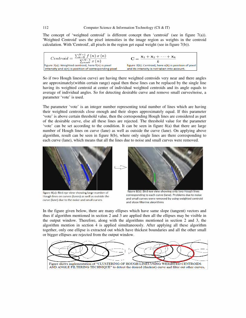
112 Computer Science & Information Technology (CS & IT)
The concept of ‘weighted centroid’
'Weighted Centroid' uses the pixel intensities in the image region as weights in the centroid
calculation. With 'Centroid', all pixels in the region get equal
So if two Hough lines(on curve) are having there weighted centroids very
are approximately(within certain range) equal then these lines can be replaced by the single line
having its weighted centroid at center of individual weighted centroids and its angle equals to
average of individual angles. So for
parameter ‘vote’ is used.
The parameter ‘vote’ is an integer number representing total number of lines which are having
their weighted centroids close enough and their slopes approximately equal. If this parameter
‘vote’ is above certain threshold value
of the desirable curve, else all these lines are rejected. The threshold value for the parameter
‘vote’ can be set according to the condition.
number of Hough lines on curve (lane) as well as outside
algorithm, result can be seen in figure 8(b), where only single lines are there corresponding to
each curve (lane), which means that all the lines d
In the figure given below, there are many ellipses which have same slope (tangent) vectors and
thus if algorithm mentioned in section 2 and 3 are applied then all the ellipses may be visible in
the output window. Therefore, along with the algorithms mentioned in section 2 and 3, the
algorithm mention in section 4 is applied simultaneously. After applying all these algorithm
together, only one ellipse is extracted out which have thickest boundaries and all the other small
or bigger ellipses are rejected from the output window.
Computer Science & Information Technology (CS & IT)
‘weighted centroid’ is different concept then ‘centroid’ (see in figure 7
Centroid' uses the pixel intensities in the image region as weights in the centroid
calculation. With 'Centroid', all pixels in the region get equal weight (see in figure 7(b)).
So if two Hough lines(on curve) are having there weighted centroids very near and there angles
are approximately(within certain range) equal then these lines can be replaced by the single line
having its weighted centroid at center of individual weighted centroids and its angle equals to
So for detecting desirable curve and remove small curves/noise, a
integer number representing total number of lines which are having
their weighted centroids close enough and their slopes approximately equal. If this parameter
‘vote’ is above certain threshold value, then the corresponding Hough lines are considered as
of the desirable curve, else all these lines are rejected. The threshold value for the parameter
‘vote’ can be set according to the condition. It can be seen in figure 8(a) that there are large
number of Hough lines on curve (lane) as well as outside the curve (lane). On applying above
algorithm, result can be seen in figure 8(b), where only single lines are there corresponding to
each curve (lane), which means that all the lines due to noise and small curves were removed.
there are many ellipses which have same slope (tangent) vectors and
thus if algorithm mentioned in section 2 and 3 are applied then all the ellipses may be visible in
the output window. Therefore, along with the algorithms mentioned in section 2 and 3, the
algorithm mention in section 4 is applied simultaneously. After applying all these algorithm
together, only one ellipse is extracted out which have thickest boundaries and all the other small
or bigger ellipses are rejected from the output window.
(see in figure 7(a)).
Centroid' uses the pixel intensities in the image region as weights in the centroid
see in figure 7(b)).
near and there angles
are approximately(within certain range) equal then these lines can be replaced by the single line
having its weighted centroid at center of individual weighted centroids and its angle equals to
detecting desirable curve and remove small curves/noise, a
integer number representing total number of lines which are having
their weighted centroids close enough and their slopes approximately equal. If this parameter
, then the corresponding Hough lines are considered as part
of the desirable curve, else all these lines are rejected. The threshold value for the parameter
It can be seen in figure 8(a) that there are large
the curve (lane). On applying above
algorithm, result can be seen in figure 8(b), where only single lines are there corresponding to
removed.
there are many ellipses which have same slope (tangent) vectors and
thus if algorithm mentioned in section 2 and 3 are applied then all the ellipses may be visible in
the output window. Therefore, along with the algorithms mentioned in section 2 and 3, the
algorithm mention in section 4 is applied simultaneously. After applying all these algorithm
together, only one ellipse is extracted out which have thickest boundaries and all the other small
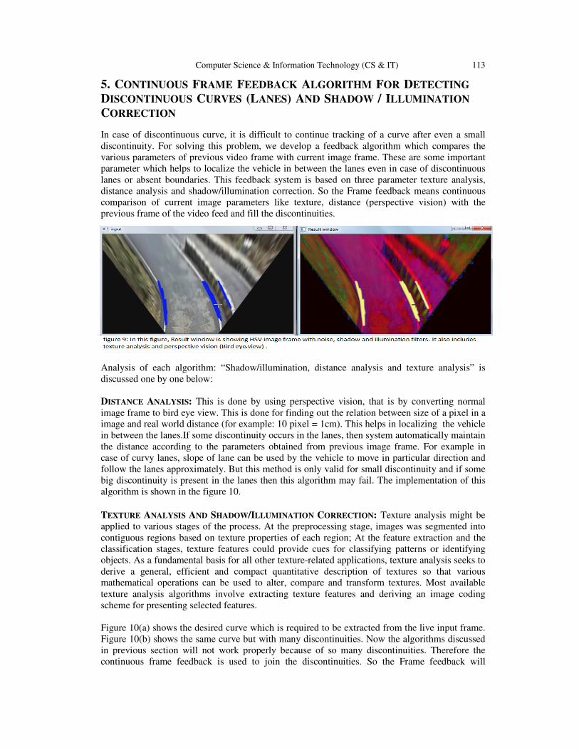
Computer Scienc
5. CONTINUOUS FRAME
DISCONTINUOUS CURVES
CORRECTION
In case of discontinuous curve, it is difficult to continue tracking of a curve after even a small
discontinuity. For solving this problem, we develop a feedback algorithm which compares the
various parameters of previous video frame with current image fra
parameter which helps to localize the vehicle in between the lanes even in case of discontinuous
lanes or absent boundaries. This
distance analysis and shadow/illumination correction.
comparison of current image parameters like
previous frame of the video feed and fill the discontinuities.
Analysis of each algorithm: “Shadow/illumination, distance analysis and texture analysis” is
discussed one by one below:
DISTANCE ANALYSIS: This is done by using perspective vision, that is by converting normal
image frame to bird eye view. This is done for finding out
image and real world distance (for example: 10 pixel = 1cm). This helps in localizing th
in between the lanes.If some discontinuity occurs in the lanes, then system automatically maintain
the distance according to the parameters obtained from previous image frame. For example in
case of curvy lanes, slope of lane can be used by the vehicle to move in particular direction and
follow the lanes approximately. But this method is only valid for small discontinu
big discontinuity is present in the lanes then this algorithm may fail. The implementation of this
algorithm is shown in the figure 10.
TEXTURE ANALYSIS AND SHADOW
applied to various stages of the process. At the preprocessing stage, images was segmented into
contiguous regions based on texture properties of each region; At the feature extraction and the
classification stages, texture featu
objects. As a fundamental basis for all other texture
derive a general, efficient and compact quantitative description of textures so that variou
mathematical operations can be used to alter, compare and transform textures. Most available
texture analysis algorithms involve extracting texture features and deriving an image coding
scheme for presenting selected features.
Figure 10(a) shows the desired curve which is required to be extracted from the live input frame.
Figure 10(b) shows the same curve but with many discontinuities. Now the algorithms discussed
in previous section will not work properly because of so many discontinuities. Therefo
continuous frame feedback is used to join the discontinuities.
Computer Science & Information Technology (CS & IT)
RAME FEEDBACK ALGORITHM FOR DETECTING
URVES (LANES) AND SHADOW / ILLUMINATION
In case of discontinuous curve, it is difficult to continue tracking of a curve after even a small
discontinuity. For solving this problem, we develop a feedback algorithm which compares the
various parameters of previous video frame with current image frame. These are some important
to localize the vehicle in between the lanes even in case of discontinuous
boundaries. This feedback system is based on three parameter texture
analysis and shadow/illumination correction. So the Frame feedback means continuous
comparison of current image parameters like texture, distance (perspective vision)
previous frame of the video feed and fill the discontinuities.
: “Shadow/illumination, distance analysis and texture analysis” is
This is done by using perspective vision, that is by converting normal
image frame to bird eye view. This is done for finding out the relation between size of a pixel in a
image and real world distance (for example: 10 pixel = 1cm). This helps in localizing th
If some discontinuity occurs in the lanes, then system automatically maintain
ording to the parameters obtained from previous image frame. For example in
case of curvy lanes, slope of lane can be used by the vehicle to move in particular direction and
follow the lanes approximately. But this method is only valid for small discontinuity and if some
big discontinuity is present in the lanes then this algorithm may fail. The implementation of this
algorithm is shown in the figure 10.
HADOW/ILLUMINATION CORRECTION: Texture analysis might be
applied to various stages of the process. At the preprocessing stage, images was segmented into
contiguous regions based on texture properties of each region; At the feature extraction and the
classification stages, texture features could provide cues for classifying patterns or identifying
objects. As a fundamental basis for all other texture-related applications, texture analysis seeks to
derive a general, efficient and compact quantitative description of textures so that variou
mathematical operations can be used to alter, compare and transform textures. Most available
texture analysis algorithms involve extracting texture features and deriving an image coding
scheme for presenting selected features.
desired curve which is required to be extracted from the live input frame.
Figure 10(b) shows the same curve but with many discontinuities. Now the algorithms discussed
in previous section will not work properly because of so many discontinuities. Therefo
continuous frame feedback is used to join the discontinuities. So the Frame feedback will
113
ETECTING
LLUMINATION
In case of discontinuous curve, it is difficult to continue tracking of a curve after even a small
discontinuity. For solving this problem, we develop a feedback algorithm which compares the
me. These are some important
to localize the vehicle in between the lanes even in case of discontinuous
texture analysis,
So the Frame feedback means continuous
texture, distance (perspective vision) with the
: “Shadow/illumination, distance analysis and texture analysis” is
This is done by using perspective vision, that is by converting normal
the relation between size of a pixel in a
image and real world distance (for example: 10 pixel = 1cm). This helps in localizing the vehicle
If some discontinuity occurs in the lanes, then system automatically maintain
ording to the parameters obtained from previous image frame. For example in
case of curvy lanes, slope of lane can be used by the vehicle to move in particular direction and
ity and if some
big discontinuity is present in the lanes then this algorithm may fail. The implementation of this
Texture analysis might be
applied to various stages of the process. At the preprocessing stage, images was segmented into
contiguous regions based on texture properties of each region; At the feature extraction and the
res could provide cues for classifying patterns or identifying
related applications, texture analysis seeks to
derive a general, efficient and compact quantitative description of textures so that various
mathematical operations can be used to alter, compare and transform textures. Most available
texture analysis algorithms involve extracting texture features and deriving an image coding
desired curve which is required to be extracted from the live input frame.
Figure 10(b) shows the same curve but with many discontinuities. Now the algorithms discussed
in previous section will not work properly because of so many discontinuities. Therefore the
So the Frame feedback will

114 Computer Science & Information Technology (CS & IT)
continuous compare current image parameters with the previous frame of the video feed and fill
the discontinuities.
6. FLOWCHART
Flowchart showing combinations of the entire algorithms explained above.

Computer Science & Information Technology (CS & IT) 115
7. CONCLUSION
In this paper we have presented new, unique and robust algorithm for detecting any type of curve
(curvy lanes) with the help of tangents of the curve. This algorithm is applicable even in adverse
conditions. This algorithm provides a general method to detect any curve with desired slopes.
First we dissect the curves into infinite Hough lines (called Curve stitching) and then by applying
various algorithm on these Hough lines , we developed a robust algorithm to detect any curvy
lanes (or in general: any curves). The implementation of concepts like mean value theorem,
clustering of Hough lines, weighted centroids, bird eye view (perspective vision), slope filtering,
shadow and illumination correction provides very accurate and efficient algorithm for curvy lane
detection or curve detection with desired slopes. I again like to mention that famous libraries like
OpenCV, Matlab are only providing functions which are able to detect some standard curves, but
this algorithm provides unique feature of detecting any curve having desired range of slopes.
Also, this algorithm reduces effect of noise, other small curves, shadow/illumination to great
extent. These algorithms can be implemented on autonomous vehicle for robust lane detection
and it can also be used in normal vehicle for speed control feedback system to avoid fatal curves
on roads. This algorithm can also be used for general purpose curve detection in various image
processing applications.’
REFERENCES
[1] Learning OpenCV, by Gary Bradski and Adrian Kaehler, Published by O’Reilly Media, Inc., 1005
Gravenstein Highway North, Sebastopol, CA 95472.
[2] On the Hough technique for curve detection; J Sklansky - IEEE Transactions on computers, 1978
[3] Probabilistic and non-probabilistic Hough transforms: overview and comparisons, by Heikki
Kälviäinen∗, Petri Hirvonen∗, Lei Xu†, Erkki Oja‡
[4] OpenCV 2.4.9.0 documentation » OpenCV Tutorials » imgproc module. Image Processing.
[5] Lane detection and tracking using B-Snake; Y Wang, EK Teoh, D Shen - Image and Vision
computing, 2004 – Elsevier
[6] Hough transform - Wikipedia, the free encyclopedia
[7] OpenCV 2 Computer Vision Application Programming Cookbook Paperback – 13 Mar, 2012, by
Robert Laganiere (Author)
[8] Lane detection by orientation and length discrimination; AHS Lai, NHC Yung - Systems, Man, and
Cybernetics, Part B: …, 2000 - ieeexplore.ieee.org.
[9] Lane detection and tracking by video sensors
[10] J Goldbeck, B Huertgen - Intelligent Transportation Systems, …, 1999 - ieeexplore.ieee.org.
[11] Lane detection using color-based segmentation, KY Chiu, SF Lin - Intelligent Vehicles Symposium,
2005. …, 2005 - ieeexplore.ieee.org.
AUTHOR
Amartansh Dubey
It is evident form past that most of the innovations due to electronics and computer
science were never dreamt by common men. I mean no one ever imagine that
mobiles, TV, 3G, nanomites, sixth sense technology, brain to brain communication,
VLSI (few vaccum tubes to millions of transistors on single chip ) could ever come
to reality and such innovations inspire and motivate me alot, as a result when most
of my friends are dreaming about good jobs and salary, i dream about publishing
great research papers, becoming part of TED, MS from places like USA, EUROPE,
etc. When i developed autonomous turret ( autonomous weapon on wheels), smart wheelchair for paralyzed
people, smart sevo motor, FM signal field strength detector, Image processing algorithms for autonomous
vehicles, i realised that i with electronics could contribute to my society and may be one day i will become
part of some great innovation. Visit my blog for more details : htttp://electronportal.blogspot.in/

116 Computer Science & Information Technology (CS & IT)
I want to be part of some great research and innovation. Sadly, here in indian society education is primarily
job and salary driven, research always comes second which leaves india far behind in electronics. For
motivating my juniors in research, i have started making some very useful tutorials which can be seen on
my blog http://electronportal.blogspot.in/. Apart from all these reasons, most important reason for my
interest in electronics is level of satisfaction i get in this field. I simply just love electronics and very much
passionate about it. Ultimate aim of my life is to become part of some great innovations and research

David C. Wyld et al. (Eds) : ITCS, CST, JSE, SIP, ARIA, DMS - 2015
pp. 117–126, 2015. © CS & IT-CSCP 2015 DOI : 10.5121/csit.2015.50112
MEDICAL IMAGE SEGMENTATION BY
TRANSFERRING GROUND TRUTH
SEGMENTATION BASED UPON TOP DOWN
AND BOTTOM UP APPROACH
Aseem Vyas and Won-Sook Lee
Department of Electrical and Computer Engineering,
University of Ottawa, Ottawa, Canada
ABSTRACT
In this paper, we present a novel method for image segmentation of the hip joint structure. The
key idea is to transfer the ground truth segmentation from the database to the test image. The
ground truth segmentation of MR images is done by medical experts. The process includes the
top down approach which register the shape of the test image globally and locally with the
database of train images. The goal of top down approach is to find the best train image for each
of the local test image parts. The bottom up approach replaces the local test parts by best train
image parts, and inverse transform the best train image parts to represent a test image by the
mosaic of best train image parts. The ground truth segmentation is transferred from best train
image parts to their corresponding location in the test image.
KEYWORDS
Shape matching, Hausdorff distance, affine transformation, Medical image segmentation,
simulated annealing optimization
1. INTRODUCTION
Image segmentation is an essential topic in the field of the image processing. The segmentation is
to highlight the object of interest in the image. The image segmentation provides the meaningful
information about an object in an image which can be further used in the different application like
face recognition, motion tracking and many more. As in the medical field, image segmentation
plays an important role. The medical image segmentation is still a difficult problem due to poor
contrast, noise and imaging artifacts. In the medical images, sometimes the boundaries of
anatomical parts are not clearly visible. To obtain good segmentation of anatomical parts, various
properties of images should be considered like intensity distribution, prior knowledge of shape.
In this paper, we solve the problem of segmentation of the hip joint structure in the MR images of
the pelvic region of human. The abnormality of shape in the hip joint structure is called
fermoacetublar impingement (FAI). The hip joint structure is the ball and socket joint. The ball is
femur and socket is acetabulum. The abnormal shape of femur and acetabulum causes the lot of
friction. Thus, the result is the damage of cartilage of femur or acetabulum in the hip joint [1] [2].
The FAI can be cured by medical surgery. For the treatment of FAI, medical practitioner
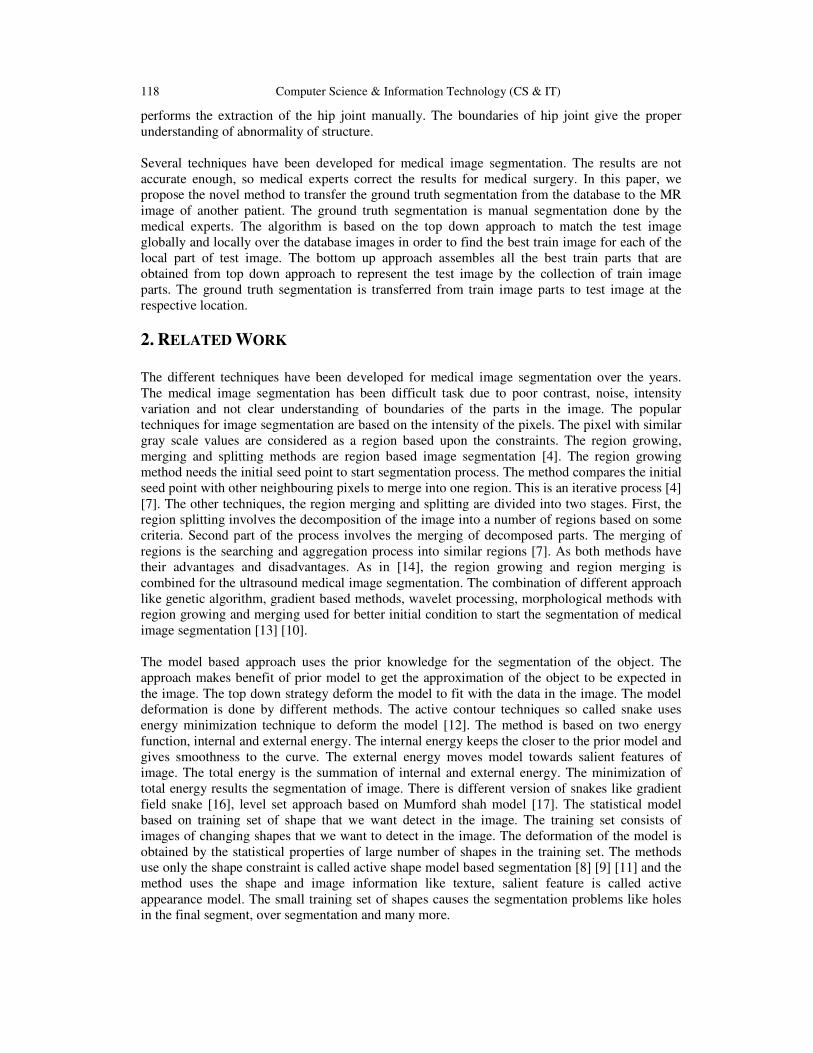
118 Computer Science & Information Technology (CS & IT)
performs the extraction of the hip joint manually. The boundaries of hip joint give the proper
understanding of abnormality of structure.
Several techniques have been developed for medical image segmentation. The results are not
accurate enough, so medical experts correct the results for medical surgery. In this paper, we
propose the novel method to transfer the ground truth segmentation from the database to the MR
image of another patient. The ground truth segmentation is manual segmentation done by the
medical experts. The algorithm is based on the top down approach to match the test image
globally and locally over the database images in order to find the best train image for each of the
local part of test image. The bottom up approach assembles all the best train parts that are
obtained from top down approach to represent the test image by the collection of train image
parts. The ground truth segmentation is transferred from train image parts to test image at the
respective location.
2. RELATED WORK
The different techniques have been developed for medical image segmentation over the years.
The medical image segmentation has been difficult task due to poor contrast, noise, intensity
variation and not clear understanding of boundaries of the parts in the image. The popular
techniques for image segmentation are based on the intensity of the pixels. The pixel with similar
gray scale values are considered as a region based upon the constraints. The region growing,
merging and splitting methods are region based image segmentation [4]. The region growing
method needs the initial seed point to start segmentation process. The method compares the initial
seed point with other neighbouring pixels to merge into one region. This is an iterative process [4]
[7]. The other techniques, the region merging and splitting are divided into two stages. First, the
region splitting involves the decomposition of the image into a number of regions based on some
criteria. Second part of the process involves the merging of decomposed parts. The merging of
regions is the searching and aggregation process into similar regions [7]. As both methods have
their advantages and disadvantages. As in [14], the region growing and region merging is
combined for the ultrasound medical image segmentation. The combination of different approach
like genetic algorithm, gradient based methods, wavelet processing, morphological methods with
region growing and merging used for better initial condition to start the segmentation of medical
image segmentation [13] [10].
The model based approach uses the prior knowledge for the segmentation of the object. The
approach makes benefit of prior model to get the approximation of the object to be expected in
the image. The top down strategy deform the model to fit with the data in the image. The model
deformation is done by different methods. The active contour techniques so called snake uses
energy minimization technique to deform the model [12]. The method is based on two energy
function, internal and external energy. The internal energy keeps the closer to the prior model and
gives smoothness to the curve. The external energy moves model towards salient features of
image. The total energy is the summation of internal and external energy. The minimization of
total energy results the segmentation of image. There is different version of snakes like gradient
field snake [16], level set approach based on Mumford shah model [17]. The statistical model
based on training set of shape that we want detect in the image. The training set consists of
images of changing shapes that we want to detect in the image. The deformation of the model is
obtained by the statistical properties of large number of shapes in the training set. The methods
use only the shape constraint is called active shape model based segmentation [8] [9] [11] and the
method uses the shape and image information like texture, salient feature is called active
appearance model. The small training set of shapes causes the segmentation problems like holes
in the final segment, over segmentation and many more.

Computer Science & Information Technology (CS & IT) 119
In the field of medical image analysis, the object recognition and boundary detection of the organ
in a medical image is very important to delineate their shape. For a proper segmentation, it is
important to segment the local and global parts of the object. The top down approach gives a
global detection and bottom up approach start from a low level and the results the object shape.
Both the approach has their own importance, without the global detection, it is difficult to get
proper local structural information. The prior model is used for searching the object in the image.
The model is transformed to find similarity with objects in the image [3] [15]. After the global
detection, the local structure matching is important to get acceptable segmentation. As in [6], the
local part based template matching is used for human detection and segmentation.
The medical image segmentation is obtained from existing algorithms still corrected by the expert
people. We develop the novel method to transfer the expert people segmentation by the shape
matching algorithm based on the hausdorff distance to extract the boundaries of hip joint structure
in the MR image of the pelvic region.
3. METHODOLOGY
Figure 1: Workflow of the system
The method is the top down approach for shape matching based on the hausdorff distance of test
image with train images and bottom up strategy to represent the test image from the collection of
best train image parts. So, the ground truth segmentation can be transferred to test image.
3.1. Hausdorff distance
The hausdorff distance is the metric to measure the degree of mismatch between two shapes of
images. The hausdorff distance is max-min distance between the two sets of points. To calculate
the distance between two images, the boundaries are extracted from both test and train image. The
edge image represents the set of points for test and train image. Given a test image A and train
image B, the hausdorff distance is defined as
Where
The h (A,B) is the directed Hausdorff distance. It is defined as by considering every point of A,
calculating the distance from that point to the closest point of B and evaluate the maximum

120 Computer Science & Information Technology (CS & IT)
among them [3]. The hausdorff distance is sensitive to the noise and outliers. The hausdorff
distance is modified to fix this problem. The parts of shapes are compared. The directed partial
hausdorff distance is defined as
,
Where denotes the Kth ranked value among the measured distances. The every point of A,
calculate the distance from that point to the closest point of B and then points of B are sorted
according to their distances and the Kth value will indicate the K of the model point of A is within
the distance of d with some points of A.
The partial hausdorff distance gives bad results with corrupted data; we need more a robust
measure to solve the problem with corrupted data. The least trimmed square (LTS-HD) hausdorff
distance is robust measure. It is defined by the linear combination of order statistics. LTS
hausdorff distance is defined as
Where k is K=f.N, the N is the number of points in the chunk of A. We used LTS-HD as a
similarity metric to detect test image model in the database of train images [5].
3.2. Simulated annealing optimization
The simulated annealing is the search algorithm which finds the optimal solution in the search
space. It is based on the probabilistic method to find the global optimum solution of the function
in the given search space. The algorithm is influenced by the annealing process of the metal in the
thermodynamics. The annealing process heats up the metal at high temperature to excite the
molecules of the metal. At high temperature, it is possible to change the structure of the metal.
The metal undergoes through the cooling process to obtain new physical structure. The
temperature is reduced gradually to obtain the desired structure of the metal. The temperature is
kept as a variable to simulate the heating and cooling process. The initial temperature and random
solution are important parameters to start the algorithm [3]. When the algorithm is at high
temperature, it will accept the more solution. This step will avoid the local optimum solution as it
comes along the path of finding a global optimum solution. The temperature of the system is
reduced gradually to work on the limited solution. The system can accept a worse solution, so
algorithm concentrate on the search area where we can find the global optimum solution. The
major advantage of the simulated annealing is not stuck in the local optima but search for the
global optimum solution.
In our system, we have used the simulated annealing optimization to minimize the LTS hausdorff
distance to detect the test image model in the train image dataset. The initial and final temperature
is very important parameter to obtain desired solution.
3.3. Database of MR images
The segmentation of MR images is divided into three categories.1) Automatic 2) semi automatic
3) manual segmentation. The automatic segmentation is based on the intensity of the pixels in the
image. The semi automatic segmentation needs human intervention to select the region of interest
for segmentation. The human can recognize the boundaries and shape of the object of interest

Computer Science & Information Technology (CS & IT) 121
more accurately than the computer algorithm [1]. The manual segmentation is most accurate
segmentation among all of them. We created a knowledge base of ground truth segmentation of
MR images of hip joint structure. The MR images are segmented manually by the medical
experts. The MR images are collected with their ground truth segmentation and then stored in the
database. We used the database images knowledge to segment the MR image of other patients.
The database images are named as train images. The knowledge 1base consists of 20 images.
4. TOP DOWN AND BOTTOM UP APPROACH
4.1. Global detection of test image
The main objective of top down approach is to detect global and local structure of the test image
in the train images. In the hausdorff distance based shape matching is used for detection of the
test image in a train image. The canny edge detection algorithm is used for the extraction of
boundaries of both test and train images. Given a test image M and train image I1 , I2 .....In, the
objective of shape matching is to obtain a transformation T to find similarity by the minimization
of hausdorff distance as the similarity metric. The affine transformation maps the point in one
plane to the other. The affine transformation parameter is scaling, rotation and translation. Let p=
(x, y) represents the point of test image, then the transformation is defined as
Where Sx and Sy are the scaling parameters in x and y direction. The translation parameters are tx
and ty in x and y direction and the rotation parameter either in a clockwise or anticlockwise
direction. The transformed point (x2, y2) is close to the train image points. The simulated annealing
search for best possible transformation in the given search space to minimize hausdorff distance
to make test image more similar to the train image. The test image is registered with all the train
images in the database. Then each of the registration gives the hausdorff distance and affine
transformation parameters. The train images are sorted in the ascending order according to the
hausdorff distance, half of the train images are selected from database for further processing. So,
out of the 20 images only 10 images are selected.
4.2. Hierarchical tree based local part registration
As in the previous section, the train images are selected with their respective transformation
parameters. The scaling and rotation is used for the transformation of the test image. Thus, the
total number of transformed images is ten. Each of the transformed test images is decomposed
into four parts as shown in figure 2. The hierarchical tree is constructed by placing decomposed
parts into tree as shown in figure 2. The tree has three levels denoted by Li, i= 0, 1, 2. Each level
has transformed test image and decomposed for the next level like level 0 (L0) which has only
transformed test image. At each level, the local parts are registered with the selected train images.
The train image is again sorted in ascending order according to the hausdorff distance obtain in
registration process of local parts. The transformed test parts at the level 1 (L1) are denoted as
Part 1, Part 2, Part 3, Part 4. Each of the tree nodes consists of 10 local parts. For example, Part_1
has 10 images and each of the Part_1 is registered with selected train image. The train images are
sorted according to the hausdorff distance and first half of the train images are selected for their
respective test image parts. For Part_1, the I10, I13, I14, I15, I16 is selected for next level registration.
The transformation obtained in L1 is used for next level registration.

122 Computer Science & Information Technology (CS & IT)
The level 2 has 80 local parts. Each of the parts of level 1 is transformed and decomposed into
four parts for the next level. The level 2 parts are represented as Part j_k. The j represents parts of
level 1 and k represent the decomposition of level 1 part into level 2.So, Part 1_2 means Part1 of
level1 is decomposed into four parts and it is the second decomposition of Part 1 of level 1.At
level 2 (L2) , the decomposed parts are registered with selected train images. For L2, rotation and
translation is used as transformation parameter for local part registration based on hausdorff
distance. The train images for L2 are sorted in ascending order according their respective
hausdorff distance. The train image with lowest hausdorff distance is selected with their
transformation as a best train image for its corresponding test image local part at level 2. Finally,
each of the local part of level 2 are transformed and matched with their best train image. So, there
are 16 local parts with their 16 best train images. We stop the decomposition of test image parts at
level 2.
Figure 2: Top down approach of shape matching
4.3. Bottom up approach
The bottom up approach aggregates all best train image parts, and represent the test image from
the collection of best train image parts. As in the previous section, each of the local part has their
corresponding best train image. For each of the local part of test images, train image part is
cropped to the same size of test image local parts at L2. The local test image parts of L2 are
replaced by the corresponding train image part. The transformation obtained after the level 2 local
part registrations is inversed and applied to the best train image part. The level 2 consists of best
train image parts which are transformed inversely. The inverse scaling parameters are 1/Sx and
1/Sy in x and y direction. The inverse rotation is negative of angle of rotation; if the top down
parameter is clock wise then inverse rotation is anti-clockwise. The –tx and ty is the inverse
translation in x and y direction. As we climb up the tree, at every level, we merge the best train
parts into one region and as we can see in the figure 3, the final image is the mosaic of best train
image parts.
The test image is symbolized by the collection of best train image parts. The database consists of
ground truth of these train images. The ground truth segmentation from the train image parts of
the test image to their corresponding location. Finally, the segmentation of test image is the
collection of the ground truth segmentation of train images.

Computer Science & Information Technology (CS & IT) 123
Figure 3: Bottom a test image to represent test image by the train image parts
5. EXPERIMENTAL RESULTS The database consists of 20 MR images of size 256 x 256 of hip joint structure with their ground
truth segmentation. The size of test image is 155 x 123. The canny edge detector is used for
extraction of boundaries of test and train images. The threshold and sigma are 0.545 and 4 for the
canny edge detector. The simulated annealing initial temperature parameter is 100. The affine
transformation parameter for global detection is 0.863≤Sx≤0.982 and 0.79≤Sy≤0.97 as a scaling
parameter in x and y direction. The rotation parameter is from -10 to 10 and translation parameter
is 0≤tx≤400 and 0≤ty≤400 in x and y direction.
(a) (b) (c)
Figure 4: (a) Test image (b) MR image database and (c) Transformed test image.

124 Computer Science & Information Technology (CS & IT)
Figure 5: The global registration of test image over train image.
(a) (b)
Figure 6: (a) Decomposed test parts at level one and (b) Local part registration.
(a) (b)
Figure 7: (a) shows local parts at level two and (b) shows its registration with train images.
Computer Science & Information Technology (CS & IT) 125
Figure 8: The segmentation of test image from ground truth data
6. CONCLUSIONS We have proposed the novel method of image segmentation of hip joint structure in MR image.
The method is to transfer ground truth segmentation from the train image database to the test
image. The train image database consists of MR images of hip joint structure with their ground
truth segmentation. The ground truth segmentation is done by medical experts. The method based
on the top down approach to register test image globally and locally with the train images. The
top down approach uses the hausdorff distance based shape registration algorithm. The objective
of the top down approach is to find the best train image for each of the local test image parts. The
bottom up approach uses the inverse transformation to match best train image parts with the
original test image and the test image is represented by the mosaic of best train image parts. The
ground truth segmentation from train image parts to their respective location of test image.
REFERENCES
[1] Chavez-Aragon A., Won-sook Lee & Vyas A., (2013) “A crowdsourcing web platform-hip joint
segmentation by non-expert contributor”, IEEE International symposium on medical measurement
and application proceedings, pp 30-354.
[2] S. Wisniewski, G.B., (2006) “Femoroacetabular impingement: An overlooked cause of hip joint”,
American Journal of Physical Medicine and Rehabilitation, No.85, pp 546-549.
[3] Rucklidge W.J., (1997) “Efficiently locating objects using hausdoff distance”, International journal of
computer vision, Vol.24, pp 251-270.
[4] Priyadarshi, S.Selvathi, D., (2007) “Survey on segmentation of liver from CT images”, IEEE
conference on advanced communication control and computing technologies, pp 1408-1421
[5] Jian-xin Knag, Nai-ming Qi, Jian-Hou, (2010) “A hybrid method combining hausdorff distance,
genetic algorithm and simulated annealing algorithm for image matching”, IEEE conference on
computer modelling and simulation, pp 435-439.
[6] Zhe Lin, Davis L.S., (2010) “Shape-based human detection and segmentation via hierarchical part-
template matching”, IEEE transaction on pattern analysis and machine intelligence, Vol.32, pp 604-
618
[7] Ansari M.A., Anand R.S., (2007) “Region based segmentation and image analysis with application to
medical imaging”, International conference on Information and communication technology in
Electrical Sciences, pp 724-729.
[8] Inamdar R.S., Ramdasi D.S., (2013) “Active appreance model for segmentation of cardiac MRI data”,
International conference on Communication and Signal Processing, pp 96-100.
[9] Kainmueller D, Lamecker H., Zachow S., Hege HC,(2009) “ An articulated statistical shape model for
hip joint segmentation”, International conference of the IEEE EMBS.
[10] Angelina S., Suresh L.P.,Veni S.H.K., (2012) “Image segmentation based on genetic algorithm for
region growth and region merging”, International conference on computing, electronics and electrical
technologies, pp 970-974.

126 Computer Science & Information Technology (CS & IT)
[11] Ying Xia, Chandra S., Salvado O., Fripp J.,(2011) “Automated MR hip bone segmentation”,
International conference on digital image computing techniques and applications, pp 25-30.
[12] J.M. Pardo, D Cabello, J Heras, (1997) “A snake for model based segmentation of biomedical
images”, Elsevier Pattern Recognition Letters, Vol. 18, pp 1529-1538.
[13] Vasilache S., van Najarian K., (2009) “A unified method based on wavelet filtering and active
contour models for segmentation of pelvic CT images”, International conference on complex medical
engineering, pp 1-5.
[14] Hui Guan, De-yu Li, Jiang-li Lin, Tian-Fu Wang, (2007) “Segmentation of ultrasound medical image
using a hybrid method”, IEEE international conference on complex medical engineering, pp 644-647.
[15] Jian-Wei Zhang, Guo-Qiang Han, Yan Wo, (2005) “ Image registration based on generalized and
mean hausdorff distance”, International conference on machine learning and cybernetics, Vol. 8, pp
5117-5121.
[16] Kazerooni A.F., Ahmadian A., Serej N.D., Rad H.S.,Saberi H., Yousefi H., Farnia P.,(2011)
“Segmentation of brain tumors in MRI images using multi-scale gradient vector flow”, IEEE
International conference of engineering in medicine and biology society, pp 7973-7976.
[17] Li-jun Zhang, Xaio-juan Wu, Zan Sheng, (2006) “A fast image segmentation approach based on level
set method”, International conference on signal processing, Vol. 2.

David C. Wyld et al. (Eds) : ITCS, CST, JSE, SIP, ARIA, DMS - 2015
pp. 127–137, 2015. © CS & IT-CSCP 2015 DOI : 10.5121/csit.2015.50113
FEATURE SELECTION: A NOVEL
APPROACH FOR THE PREDICTION OF
LEARNING DISABILITIES IN SCHOOL-
AGED CHILDREN
Sabu M.K
Department of Computer Applications,
M.E.S College, Marampally, Aluva, Kerala, India [email protected]
ABSTRACT
Feature selection is a problem closely related to dimensionality reduction. A commonly used
approach in feature selection is ranking the individual features according to some criteria and
then search for an optimal feature subset based on an evaluation criterion to test the optimality.
The objective of this work is to predict more accurately the presence of Learning Disability
(LD) in school-aged children with reduced number of symptoms. For this purpose, a novel
hybrid feature selection approach is proposed by integrating a popular Rough Set based feature
ranking process with a modified backward feature elimination algorithm. The approach follows
a ranking of the symptoms of LD according to their importance in the data domain. Each
symptoms significance or priority values reflect its relative importance to predict LD among the
various cases. Then by eliminating least significant features one by one and evaluating the
feature subset at each stage of the process, an optimal feature subset is generated. The
experimental results shows the success of the proposed method in removing redundant
attributes efficiently from the LD dataset without sacrificing the classification performance.
KEYWORDS
Rough Set Theory, Data Mining, Feature Selection, Learning Disability, Reduct.
1. INTRODUCTION
Learning Disability (LD) is a neurological disorder that affects a child’s brain. It causes trouble
in learning and using certain skills such as reading, writing, listening and speaking. A possible
approach to build computer assisted systems to handle LD is: collect a large repository of data
consisting of the signs and symptoms of LD, design data mining algorithms to identify the
significant symptoms of LD and build classification models based on the collected data to classify
new unseen cases. Feature selection is an important data mining task which can be effectively
utilized to develop knowledge based tools in LD prediction. Feature selection process not only
reduces the dimensionality of the dataset by preserving the significant features but also improves
the generalization ability of the learning algorithms.
Data mining, especially feature selection is an exemplary field of application where Rough Set
Theory (RST) has demonstrated its usefulness. RST can be utilized in this area as a tool to
discover data dependencies and reduce the number of attributes of a dataset without considering

128 Computer Science & Information Technology (CS & IT)
any prior knowledge and using only the information contained within the dataset alone [2]. In
this work, RST is employed as a feature selection tool to select most significant features which
will improve the diagnostic accuracy by SVM. For this purpose, a popular Rough Set based
feature ranking algorithm called PRS relevance approach is implemented to rank various
symptoms of the LD dataset. Then by integrating this feature ranking technique with backward
feature elimination [15], a new hybrid feature selection technique is proposed. A combination of
four relevant symptoms is identified from the LD dataset through this approach which gives the
same classification accuracy compared to the whole sixteen features. It implies that these four
features were worthwhile to be taken close attention by the physicians or teachers handling LD
when they conduct the diagnosis.
The rest of the paper is organized as follows. A review of Rough Set based feature ranking
process is given in section 2. In section 3, conventional feature selection procedures are
described. A brief description on Learning Disability dataset is presented in Section 4. Section
5 presents the proposed approach of feature selection process. Experimental results are reported
in Section 6. A discussion of the experimental results is given in Section 7. The last section
concludes this research work.
2. ROUGH SET BASED ATTRIBUTE RANKING
Rough Set Theory (RST) proposed by Z. Pawlak is a mathematical approach to intelligent data
analysis and data mining. RST is concerned with the classificatory analysis of imprecise,
uncertain or incomplete information expressed in terms of data acquired from experience. In
RST all computations are done directly on collected data and performed by making use of the
granularity structure of the data. The set of all indiscernible (similar) objects is called an
elementary set or a category and forms a basic granule (atom) of the knowledge about the data
contained in the dataset. The indiscernibility relation generated in this way is the mathematical
basis of RST [18].
The entire knowledge available in a high dimensional dataset is not always necessary to define
various categories represented in the dataset. Though the machine learning and data mining
techniques are suitable for handling data mining problems, they may not be effective for handling
high dimensional data. This motivates the need for efficient automated feature selection
processes in the area of data mining. In RST, a dataset is always termed as a decision table. A
decision table presents some basic facts about the Universe along with the decisions (actions)
taken by the experts based on the given facts. An important issue in data analysis is whether the
complete set of attributes given in the decision table are necessary to define the knowledge
involved in the equivalence class structure induced by the set of all attributes. This problem
arises in many practical applications and will be referred to as knowledge reduction. With the
help of RST, we can eliminate all superfluous attributes from the dataset preserving only the
indispensable attributes [18]. In reduction of knowledge, the basic roles played by two
fundamental concepts in RST are reduct and core. A reduct is a subset of the set of attributes
which by itself can fully characterize the knowledge in the given decision table. A reduct keeps
essential information of the original decision table. In a decision table there may exist more than
one reduct. The set of attributes which is common to all reducts is called the core [18]. The core
may be thought of as the set of indispensable attributes which cannot be eliminated while
reducing the knowledge involved in the information system. Elimination of a core attribute from
the dataset causes collapse of the category structure given by the original decision table. To
determine the core attributes, we take the intersection of all the reducts of the information system.
In the following section, a popular and more effective reduct based feature ranking approach
known as PRS relevance method [19] is presented. In this method, the ranking is done with the

Computer Science & Information Technology (CS & IT) 129
help of relevance of each attribute/feature calculated by considering its frequency of occurrence
in various reducts generated from the dataset.
2.1. Proportional Rough Set (PRS) Relevance Method
This is an effective Rough Set based method for attribute ranking proposed by Maria Salamó and
López-Sánchez [19]. The concept of reducts is used as the basic idea for the implementation of this
approach. The same idea is also used by Li and Cercone to rank the decision rules generated from
a rule mining algorithm [20, 21, 22, 23]. There exist multiple reduct for a dataset. Each reduct is a
representative of the original data. Most data mining operations require only a single reduct for
decision making purposes. But selecting any one reduct leads to the elimination of representative
information contained in all other reducts. The main idea behind this reduct based feature ranking
approach is the following: the more frequent a conditional attribute appears in the reducts and the
more relevant will be the attribute. Hence the number of times an attribute appears in all reducts
and the total number of reducts determines the significance (priority) of each attribute in
representing the knowledge contained in the dataset. This idea is used for measuring the
significance of various features in PRS relevance feature ranking approach [19]. With the help of
these priority values the features available in the dataset can be arranged in the decreasing order
of their priority.
3. FEATURE SELECTION
The Feature selection is a search process that selects a subset of significant features from a data
domain for building efficient learning models. Feature selection is closely related to
dimensionality reduction. Most of the dataset contain relevant as well as irrelevant and redundant
features. Irrelevant and redundant features do not contribute anything to determine the target
class and at the same time deteriorates the quality of the results of the intended data mining task.
The process of eliminating these types of features from a dataset is referred to as feature
selection. In a decision table, if a particular feature is highly correlated with decision feature, then
it is relevant and if it is highly correlated with others, it is redundant. Hence the search for a good
feature subset involves finding those features that are highly correlated with the decision feature
but uncorrelated with each other [1]. Feature selection process reduces the dimensionality of the
dataset and the goal of dimensionality reduction is to map a set of observations from a high
dimensional space M into a low dimensional space m (m<<M) by preserving the semantics of the
original high dimensional dataset. Let I = (U, A) be an information system (dataset), where U =
{x1, x2, …, xn} be the set of objects and A = {a1, a2, …, aM} be the set of attributes used to
characterize each object in I. Hence each object xi in the information system can be represented
as an M dimension vector [a1(xi), a2(xi), …, aM(xi)], where aj(xi) yields the jth (j = 1, 2, 3, …, M)
attribute value of the ith (i = 1, 2, 3, …., n) data object. Dimensionality reduction techniques
transform the given dataset I of size n × M into a new low dimensional dataset Y of size n × m.
While constructing a feature selection method, two different factors namely search strategies and
evaluating measures [2] are to be considered. Commonly used search strategies are complete or
exhaustive [3], heuristic [4] and random [5][6]. In general feature selection methods are based on
some exhaustive approaches which are quite impractical in many cases, especially for high
dimensional datasets, due to the high computational cost involved in the searching process [25].
To reduce this complexity, as an alternate solution strategy, heuristic or random search methods
are employed in modern feature selection algorithms.
Based on the procedures used for evaluating the scalability of the generated subset, heuristic or
random search methods are further classified into three – classifier specific or wrapper methods
[7][8][9][10][11], classifier independent or filter methods [12][13][14] and hybrid models [15]

130 Computer Science & Information Technology (CS & IT)
which combines both filter and wrapper approach to achieve better classification performance. In
a classifier specific feature selection method, the quality of the selected features is evaluated with
the help of a learning algorithm and the corresponding classification accuracy is determined. If it
satisfies the desired accuracy, the selected feature subset is considered as optimal; otherwise it is
modified and the process is repeated for a better one. The process of feature selection using
wrapper (classifier specific) approach is depicted in Figure 1. Even though the wrapper method
may produce better results, it is computationally expensive and can encounter problems while
dealing with huge dataset.
Figure 1: Wrapper approach to feature selection
In the case of classifier independent method, to evaluate the significance of selected features one
or more of classifier independent measures such as inter class distance [12], mutual information
[16][17] and dependence measure [13][18] are employed. In this approach, the process of feature
selection is treated as a completely independent pre-processing operation. As an outcome of this
pre-processing, irrelevant/noisy attributes are filtered. All filter based methods use heuristics
based on general characteristics of the data rather than a learning algorithm to evaluate the
optimality of feature subsets. As a result, filter methods are generally much faster than wrapper
methods. Since this method does not depend on any particular learning algorithm, it is more
suitable in managing high dimensionality of the data.
In the case of hybrid model, as a first step, features are ranked using some distance criterion or
similarity measure and then with the help of a wrapper model an optimal feature subset is
generated. The method usually starts with an initial subset of features heuristically selected
beforehand. Then features are added (forward selection) or removed (backward elimination)
iteratively until an optimal feature subset is obtained.
4. LEARNING DISABILITY DATASET
Learning disability (LD) is a neurological condition that affects the child’s brain resulting in
difficulty in learning and using certain skills such as reading, writing, listening, speaking and
reasoning. Learning disabilities affect children both academically and socially and about 10% of
children enrolled in schools are affected with this problem. With the right help at the right time,
children with learning disabilities can learn successfully. Identifying students with LD and
assessing the nature and depth of LD is essential for helping them to get around LD. As nature
and symptoms of LD may vary from child to child, it is difficult to access LD. A variety of tests
are available for evaluating LD. Also there are many approaches for managing LD by teachers as
well as parents.
To apply the proposed methodology on a real world dataset, a dataset consisting of the signs and
symptoms of the learning disabilities in school age children is selected. It is collected from
various sources which include a child care clinic providing assistance for handling learning
disability in children and three different schools conducting such LD assessment studies. This
dataset is helpful to determine the existence of LD in a suspected child. It is selected with a view
to provide tools for researchers and physicians handling learning disabilities to analyze the data
and to facilitate the decision making process.

Computer Science & Information Technology (CS & IT) 131
The dataset contains 500 student records with 16 conditional attributes as signs and symptoms of
LD and the existence of LD in a child as decision attribute. Various signs and symptoms
collected includes the information regarding whether the child has any difficulty in reading (DR),
any difficulty with spelling (DS), any difficulty with handwriting (DH) and so on. There are no
missing values or inconsistency exists in the dataset. Table 1 gives a portion of the dataset used
for the experiment. In this table t represents the attribute value true and f represents the attribute
value false. Table 2 gives key used for representing the symptoms and its abbreviations.
Table 1: Learning Disability (LD) dataset
Table 2: Key used for representing the symptoms of LD
Key/ Abbreviations Symptoms Key/
Abbreviations Symptoms
DR Difficulty with Reading LM Lack of Motivation
DS Difficulty with Spelling DSS Difficulty with Study
Skills
DH Difficulty with Handwriting DNS Does Not like School
DWE Difficulty with Written
Expression DLL
Difficulty in Learning a
Language
DBA Difficulty with Basic
Arithmetic
DLS Difficulty in Learning a
Subject
DHA Difficulty with Higher
Arithmetic skills STL Is Slow To Learn
DA Difficulty with Attention RG Repeated a Grade
ED Easily Distracted LD Learning Disability
DM Difficulty with Memory

132 Computer Science & Information Technology (CS & IT)
5. PROPOSED APPROACH The proposed method of feature selection follows a hybrid approach which utilizes the
complementary strength of wrapper and filter approaches. Before feature selection begins, each
feature is evaluated independently with respect to the class to identify its significance in the data
domain. Features are then ranked in the decreasing order of their significance[26]. To calculate
the significance and to rank various features of the LD dataset, in this work, PRS relevance
approach is used. To explain the feature ranking process, consider a decision table T = {U, A, d},
where U is the non-empty finite set of objects called the Universe, A = {a1, a2, …, an} be the non-
empty finite set of conditional attributes/features and d is the decision attribute. Let {r1, r2,…, rp} be
the set of reducts generated from T. Then, for each conditional attribute ai ∈ A, reduct based
attribute priority/significance ( )iaβ is defined as [19, 20, 21]:
{ }ni
p
pjrara
jij
i ,...,3,2,1,,...,3,2,1,
)( ==∈
=β
1
where the numerator of the Eq. 1 gives the occurrence frequency of the attribute ai in various
reducts.
From Eq. 1 it is clear that an attribute a not appearing in any of the reducts has priority value β(a)
= 0. For an attribute a, which is a member of core of the decision table has a priority value β(a) =
1. For the remaining attributes the priority values are proportional to the number of reducts in
which the attribute appear as a member. These reduct based priority values will provide a
ranking for the considered features.
After ranking the features, search process start with all available features and successfully remove
least significant features one by one (backward elimination) after evaluating the influence of this
feature in the classification accuracy until the selected feature subset gives a better classification
performance. When a certain feature is eliminated, if there is no change in the current best
classification accuracy the considered feature is redundant. If the classification accuracy is
increased as a result of elimination, the removed feature is considered as a feature with negative
influence on the classification accuracy. In these two cases, the selected feature is permanently
removed from the feature subset; otherwise it is retained. Feature evaluation starts by considering
the classification accuracy obtained from all available features as the current best accuracy. The
search terminates when no single attribute deletion contributes any improvement in the current
best classification accuracy. At this stage, the remaining feature subset is considered as optimal.
For classification, Sequential Minimal Optimization (SMO) algorithm using the polynomial
kernel is used in this work. It is implemented through Weka data mining tool kit [24]. This
algorithm is used for the prediction of LD because it is simple, easy to implement and generally
faster. The proposed feature selection algorithm FeaSel is presented below. The algorithm
accepts the ranked set of features obtained from the PRS relevance approach as input and
generates an optimal feature subset consisting of the significant features as output. The overall
feature selection process is represented in figure 2.
Algorithm FeaSel(Fn, Y, n, Xn)
//Fn ={f1, f2,...,fn}– Set of features obtained from PRS relevance approach ranked in
descending order of their significance.
//Y – class; n – total number of features.
// Xn – The optimal feature subset.
{

Computer Science & Information Technology (CS & IT) 133
Xn=Fn;
max_acc=acc(Fn,Y); //acc() returns the classification accuracy given by the classifier
for (i=n to 1 step -1) do
{
Fn=Fn-{fi};
curr_acc=acc(Fn, Y);
if (curr_acc==max_acc)
Xn=Fn;
else if (curr_acc>max_acc)
{
Xn=Fn;
max_acc=curr_acc;
}
else
Xn=Fn∪{fi};
Fn=Xn;
}
return(Xn, max_acc);
}
Figure 2: Block diagram of the feature selection process

134 Computer Science & Information Technology (CS & IT)
6. EXPERIMENTAL ANALYSIS AND RESULTS In order to implement the PRS relevance approach to rank the features, as a first step of the
process, various reducts are generated from the LD dataset. For this purpose, the discernibility
matrix approach of Rough Sets Data Explorer software package ROSE2 is used which generates
63 reducts from the original LD dataset. Then frequencies of various features occurring in these
reducts are computed. These frequencies are given in Table 3. Based on these frequencies and by
applying Eq. 1, the priority/significance values of various features are calculated. Ranked features
as per their significance are shown in Table 4.
Table 3: Frequencies of various attributes in reducts
Feature Frequency Feature Frequency
DR 63 DSS 18
DS 34 DNS 23
DWE 32 DHA 21
DBA 41 DH 16
DA 44 DLL 50
ED 63 DLS 27
DM 63 RG 36
LM 41 STL 27
Table 4: Attributes with priority values
Rank Feature Significance Rank Feature Significance
1 DR 1 9 DS 0.5397
2 ED 1 10 DWE 0.5079
3 DM 1 11 DLS 0.4286
4 DLL 0.7937 12 STL 0.4286
5 DA 0.6984 13 DNS 0.3651
6 LM 0.6508 14 DHA 0.3333
7 DBA 0.6508 15 DSS 0.2857
8 RG 0.5714 16 DH 0.2540
For feature selection using the proposed algorithm, the classification accuracy of the whole LD
dataset with all available features is determined first. In the feature selection algorithm the
construction of the best feature subset is mainly based on this value. Then, the set of features
ranked using PRS relevance approach is given to the proposed feature selection algorithm FeaSel.
Since the features are ranked in decreasing order of significance, features with lower ranks gets
eliminated during initial stages. The algorithm starts with all features of LD and in the first
iteration the algorithm selects lowest ranked feature DH as a test feature. Since there is no
change occurs in the original classification accuracy while eliminating this feature, it is

Computer Science & Information Technology (CS & IT) 135
designated as redundant and hence it is permanently removed from the feature set. The same
situation continues for the features DSS, DHA, DNS, STL, and DLS selected in order from right
to left from the ranked feature set and hence all these features are removed from the feature set.
But when selecting the next feature DWE, there is a reduction in the classification accuracy
which signifies the influence of this feature in determining the classification accuracy and hence
this feature is retained in the feature set. The process is continued until all features are evaluated.
The performance of various symptoms of LD during the feature selection process is depicted in
figure 3.
Figure 3. Influence of various symptoms in classification
After evaluating all features of the LD dataset, the algorithm retains the set of features {DWE,
DS, DLL, DM}. These four features are significant because all other features can be removed
from the LD dataset without affecting the classification performance. Table 5 shows the results
obtained from the classifier before and after the feature selection process. To determine the
accuracy 10 fold cross validation is used.
Table 5: Classification results given by SMO
Various cases Dataset prior to perform
feature selection
Dataset reduced using the
proposed approach
No. of features 16 4
Classification accuracy (%) 98.6 98.6
Time taken to build the model (Sec.) 0.11 0.01
7. DISCUSSION
From the experimental results presented in Table 5 it is clear that, in the case of the proposed
approach a 75% reduction in the dataset does not affect the classification accuracy. It follows
that the original dataset contains about 75% redundant attributes and the feature selection
approach presented is efficient in removing these redundant attributes without affecting the
98.6 98.6 98.6 98.6 98.6 98.6
97.4
98
98.6 98.6 98.6 98.6
96.6
98.498.6 98.6
DH DSS DHA DNS STL DLS DWE DS RG DBA DM DA DLL DM ED DR
Classification Accuracy (%)

136 Computer Science & Information Technology (CS & IT)
classification accuracy. From the comparison of results, it can be seen that when using the
selected significant features for classification, the time taken to build the learning model is also
greatly improved. This shows that in an information system there are some non-relevant features
and identifying and removing these features will enable learning algorithms to operate faster. In
other words, increasing the number of features in a dataset may not be always helpful to increase
the classification performance of the data. Increasing the number of features progressively may
result in reduction of classification rate after a peak. This is known as peaking phenomenon.
8. CONCLUSION
In this paper, a novel hybrid feature selection approach is proposed to predict the Learning
Disability in a cost effective way. The approach follows a method of assigning priorities to
various symptoms of the LD dataset based on the general characteristics of the data alone. Each
symptoms priority values reflect its relative importance to predict LD among the various cases.
By ranking these symptoms in the decreasing order of their significance, least significant features
are eliminated one by one by considering its involvement in predicting the learning disability.
The experimental result reveals the need of feature selection in classification to improve the
performance such as speed of learning and predictive accuracy. With the help of the proposed
method, redundant attributes can be removed efficiently from the LD dataset without sacrificing
the classification performance.
REFERENCES
[1] Richard Jensen (2005) Combining rough and fuzzy sets for feature selection, Ph.D thesis from
Internet.
[2] Yumin Chen, Duoqian Miao & Ruizhi Wang, (2010) “A Rough Set approach to feature selection
based on ant colony optimization”, Pattern Recognition Letters, Vol. 31, pp. 226-233.
[3] Petr Somol, Pavel Pudil & Josef Kittler, (2004) “Fast Branch & Bound Algorithms for Optimal
Feature Selection”, IEEE Transactions on Pattern Analysis and Machine Intelligence, Vol. 26, No. 7,
pp. 900-912.
[4] Ning Zhong, Juzhen Dong & Setsuo Ohsuga, (2001) “Using Rough Sets with heuristics for feature
selection”, Journal of Intelligence Information systems, Vol. 16, pp.199-214.
[5] Raymer M L,Punch W F, Goodman E D,Kuhn L A & Jain A K, (2000) “Dimensionality Reduction
Using Genetic Algorithms”, IEEE Trans. Evolutionary Computation, Vol.4, No.2, pp. 164-171.
[6] Carmen Lai, Marcel J.T. Reinders & Lodewyk Wessels, (2006) "Random subspace method for
multivariate feature selection”, Pattern Recognition letters, Vol. 27, pp. 1067-1076.
[7] Ron Kohavi & Dan Sommerfield, (1995) ”Feature subset selection using the wrapper method: Over
fitting and dynamic search space topology”, Proceedings of the First International Conference on
Knowledge Discovery and Data Mining, pp. 192-197.
[8] Isabelle Guyon, Jason Weston, Stephen Barnhill & Vladimir Vapnik, (2002) “Gene selection for
cancer classification using support vector machines”, Machine Learning, Kluwer Academic
Publishers, Vol. 46, pp. 389-422.
[9] Neumann J, Schnörr C & Steidl G, (2005) “Combined SVM based feature selection and
classification”, Machine Learning, Vol.61, pp.129-150.
[10] Gasca E,Sanchez J S & Alonso R, (2006) “Eliminating redundancy and irrelevance using a new
MLP based feature selection method”, Pattern Recognition, Vol. 39, pp. 313-315.
[11] Zong-Xia Xie, Qing-Hua Hu & Da-Ren Yu, (2006) “Improved feature selection algorithm base on
SVM and Correlation”, LNCS, Vol. 3971, pp. 1373-1380.
[12] Kira K & Rendell L A, (1992) “The feature selection problem: Traditional methods and a new
algorithm”, Proceedings of the International conference AAAI-92, San Jose, CA, pp. 129-134.
[13] Mondrzejewski M, (1993) “ Feature selection using Rough Set theory” , Proceedings of the European
conference on Machine learning ECML’93, Springer-Verlag, pp. 213-226.
[14] Manoranjan Dash & Huan Liu, (2003) “Consistency based search in feature selection”, Artificial
Intelligence, Vpl.151, pp. 155-176.
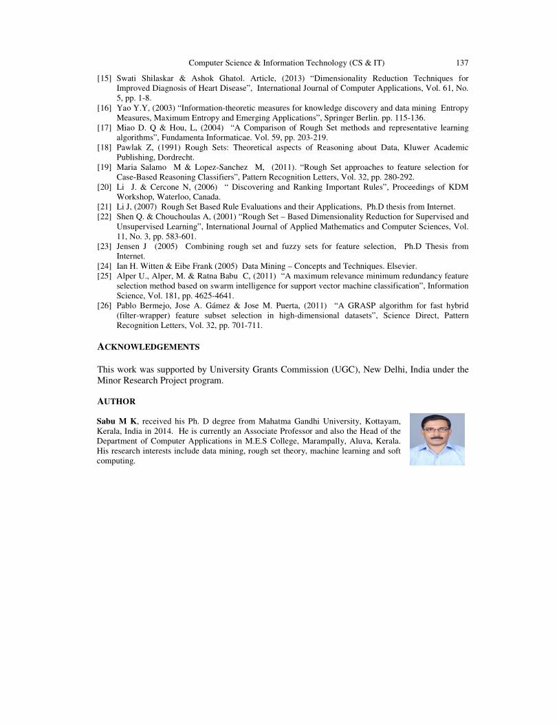
Computer Science & Information Technology (CS & IT) 137
[15] Swati Shilaskar & Ashok Ghatol. Article, (2013) “Dimensionality Reduction Techniques for
Improved Diagnosis of Heart Disease”, International Journal of Computer Applications, Vol. 61, No.
5, pp. 1-8.
[16] Yao Y.Y, (2003) “Information-theoretic measures for knowledge discovery and data mining Entropy
Measures, Maximum Entropy and Emerging Applications”, Springer Berlin. pp. 115-136.
[17] Miao D. Q & Hou, L, (2004) “A Comparison of Rough Set methods and representative learning
algorithms”, Fundamenta Informaticae. Vol. 59, pp. 203-219.
[18] Pawlak Z, (1991) Rough Sets: Theoretical aspects of Reasoning about Data, Kluwer Academic
Publishing, Dordrecht.
[19] Maria Salamo M & Lopez-Sanchez M, (2011). “Rough Set approaches to feature selection for
Case-Based Reasoning Classifiers”, Pattern Recognition Letters, Vol. 32, pp. 280-292.
[20] Li J. & Cercone N, (2006) “ Discovering and Ranking Important Rules”, Proceedings of KDM
Workshop, Waterloo, Canada.
[21] Li J, (2007) Rough Set Based Rule Evaluations and their Applications, Ph.D thesis from Internet.
[22] Shen Q. & Chouchoulas A, (2001) “Rough Set – Based Dimensionality Reduction for Supervised and
Unsupervised Learning”, International Journal of Applied Mathematics and Computer Sciences, Vol.
11, No. 3, pp. 583-601.
[23] Jensen J (2005) Combining rough set and fuzzy sets for feature selection, Ph.D Thesis from
Internet.
[24] Ian H. Witten & Eibe Frank (2005) Data Mining – Concepts and Techniques. Elsevier.
[25] Alper U., Alper, M. & Ratna Babu C, (2011) “A maximum relevance minimum redundancy feature
selection method based on swarm intelligence for support vector machine classification”, Information
Science, Vol. 181, pp. 4625-4641.
[26] Pablo Bermejo, Jose A. Gámez & Jose M. Puerta, (2011) “A GRASP algorithm for fast hybrid
(filter-wrapper) feature subset selection in high-dimensional datasets”, Science Direct, Pattern
Recognition Letters, Vol. 32, pp. 701-711.
ACKNOWLEDGEMENTS
This work was supported by University Grants Commission (UGC), New Delhi, India under the
Minor Research Project program.
AUTHOR
Sabu M K, received his Ph. D degree from Mahatma Gandhi University, Kottayam,
Kerala, India in 2014. He is currently an Associate Professor and also the Head of the
Department of Computer Applications in M.E.S College, Marampally, Aluva, Kerala.
His research interests include data mining, rough set theory, machine learning and soft
computing.

138 Computer Science & Information Technology (CS & IT)
INTENTIONAL BLANK

David C. Wyld et al. (Eds) : ITCS, CST, JSE, SIP, ARIA, DMS - 2015
pp. 139–145, 2015. © CS & IT-CSCP 2015 DOI : 10.5121/csit.2015.50114
MULTICLASS RECOGNITION WITH
MULTIPLE FEATURE TREES
Guan-Lin Li, Jia-Shu Wang, Chen-Ru Liao, Chun-Yi Tsai, and
Horng-Chang Yang
Department of Computer Science and Information Engineering,
National Taitung University, Taiwan, R.O.C. {u10011135,u10011147,u10011121}@ms100.nttu.edu.tw;
{cytsai, hcyang}@nttu.edu.tw
ABSTRACT
This paper proposes a multiclass recognition scheme which uses multiple feature trees with an
extended scoring method evolved from TF-IDF. Feature trees consisting of different feature
descriptors such as SIFT and SURF are built by the hierarchical k-means algorithm. The
experimental results show that the proposed scoring method combing with the proposed
multiple feature trees yields high accuracy for multiclass recognition and achieves significant
improvement compared to methods using a single feature tree with original TF-IDF.
KEYWORDS
SIFT, SURF, K-means, TF-IDF
1. INTRODUCTION
For machine intelligent applications, one of the critical issues is to achieve high accuracy in
multi-object recognition. This paper, motivated by Nister’s previous work[3], proposes an
algorithm comprising multiple hierarchical k-means feature trees with an improved TF-IDF[4]
scheme. The TF-IDF scheme takes account of not only the occurrence frequency of an item /
feature but also the inverse of the frequency of documents containing the item/features to the total
document. Such an item/feature is apparently good for distinguishing objects from multiple
classes. In our study, the proposed method with improved TF-IDF scheme and multiple feature
trees significantly improves the accuracy of recognizing multiple objects.
2. RELATED RESEARCH
For decades, feature descriptors are widely used in image matching and object recognition
applications. One of the classical descriptors is the state-of-the-art SIFT[2] scheme. In the SIFT
scheme, local features are detected and extracted by looking for optima in the pyramid of scale
spaces generated by the difference of Gaussian (DoG) method. Each SIFT feature consists of
orientations computed based on the local image gradient directions around a detected optimum.
As the SIFT descriptor is proved efficient and effective for image matching, object recognition,
motion tracking, and related fields in machine intelligence, various adaptations are proposed
Similar to SIFT, the SURF scheme proposed by Bay[5] generates the pyramid of scale spaces by
discrete wavelet transform and approximates the determinant of Hessian blob detector by an
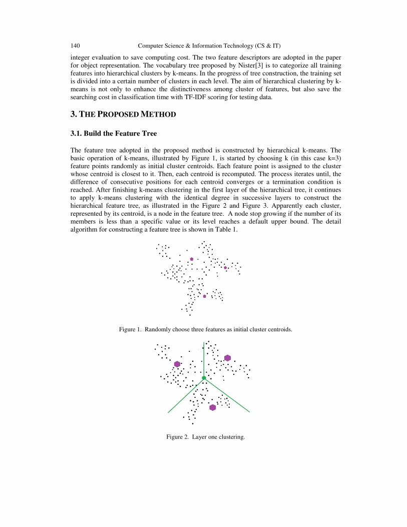
140 Computer Science & Information Technology (CS & IT)
integer evaluation to save computing cost. The two feature descriptors are adopted in the paper
for object representation. The vocabulary tree proposed by Nister[3] is to categorize all training
features into hierarchical clusters by k-means. In the progress of tree construction, the training set
is divided into a certain number of clusters in each level. The aim of hierarchical clustering by k-
means is not only to enhance the distinctiveness among cluster of features, but also save the
searching cost in classification time with TF-IDF scoring for testing data.
3. THE PROPOSED METHOD
3.1. Build the Feature Tree
The feature tree adopted in the proposed method is constructed by hierarchical k-means. The
basic operation of k-means, illustrated by Figure 1, is started by choosing k (in this case k=3)
feature points randomly as initial cluster centroids. Each feature point is assigned to the cluster
whose centroid is closest to it. Then, each centroid is recomputed. The process iterates until, the
difference of consecutive positions for each centroid converges or a termination condition is
reached. After finishing k-means clustering in the first layer of the hierarchical tree, it continues
to apply k-means clustering with the identical degree in successive layers to construct the
hierarchical feature tree, as illustrated in the Figure 2 and Figure 3. Apparently each cluster,
represented by its centroid, is a node in the feature tree. A node stop growing if the number of its
members is less than a specific value or its level reaches a default upper bound. The detail
algorithm for constructing a feature tree is shown in Table 1.
Figure 1. Randomly choose three features as initial cluster centroids.
Figure 2. Layer one clustering.

Computer Science & Information Technology (CS & IT) 141
Figure 3. Layer two clustering.
Table 1. Build the Feature Tree
Input :
1. P: input feature data
2. H: number of tree layer
3. T: initial feature tree
Output : 1. hktree: the output feature tree
Temporal:
1. Hktree : type definition of the feature tree, owning clustering function to save
center or leaf node data
2. C : the set of cluster centers
3. Kmeans(P) : k-means processing for input data and returning centers
4. A(C,P) : assigning data to the center closest to it, and returning data clusters
Hktree HKTree(P,H,T){
Hktree hktree
C = Kmeans(P)
hktree.group = A(C,P)
IF P.size > limit or T.layer < limit {
T→next = hktree
HKTree(hktree.group,H+1,T→next)
}
Else
Return hktree
}
3.2. Searching
To search an image in an image base, the image is represented by a features vector which is
compared with the features of the feature tree built in the last section as the inverted-index file of
the image base. Each feature is categorized to a cluster by following the path from the root to the
leaf node, of which each node has the closest distance to the input feature.

142 Computer Science & Information Technology (CS & IT)
3.3. Scoring
3.3.1. Weighted TF-IDF
The first attempt that we adopt for scoring is the weighted TF-IDF approach based on the original
TF-IDF scheme. The scoring policy is defined as follows. Let �� denote the total number of
features that reaches the leaf node � from an input image. Let � denote the total number of image
classes, ��� denote the number of all features of a specific image class � clustered in the leaf node
�, �� denote the number of all features clustered in the leaf node �, denote the total number of
leaf nodes, and � denote the total number of leaf nodes containing the specific image class �.
Then ���/�� is the weighting value, and the natural log of /� is the IDF value. Let � ������ denote the score of the image class �. The searching algorithm along with the scoring policy
defined in eq. (1) is shown in Table 2. After each feature extracted from an input image reaches
the leaf node that it belongs to, the total score for each candidate image class can be evaluated
respectively.
Table 2 : Algorithm for searching and scoring
FeatureTree Tree
Queue Layer=Tree.root
Queue Feature = TheSetofTotalPoints
DO{
Node node = Layer.dequeue()
Point points = Feature.dequeue()
IF node != leaf_node {
Assign points to k childs of node
FOR i=1 to k{
Layer.enqueue(childs[i])
Feature.enqueue(points[i])
}
}
ELSE{
FOR i=1 to N
FOR j=1 to M
��������+= �� × �����
× ! " #!�
$ (')
}
}WHILE node is not null
3.3.2. VT(vocabulary tree)
The vocabulary tree(VT)[3] uses the total number of features that reaches the leaf node � from an
input image as the TF value, denoted by ��. Let ) denote the total number of all features in the
dataset. Then, the second scoring policy adopted for experiment is defined as in eq. (2).
��������+= �� × ��� × ! * +��
, (-)

Computer Science & Information Technology (CS & IT) 143
3.3.3. Proposed Scoring Method
The proposed method for scoring adopts identical TF definition in method (a), but improves the
IDF. Let )� denote the total number of features of a specific image class �. Then the improved
IDF is defined as the natural log of )/)� to imply that classes with rare features are important.
That is, the scoring policy is defined as in eq. (3). The design concern for the proposed scoring
method is to generally consider the impact of rare features from the aspect of the whole dataset.
��������+= �� × �����
× ! " ++�
$ (.)
3.4. Proposed Multiple Tree Searching
With the three scoring policies, we design two additional multiple-feature-trees schemes, SIFT⊕SURF and SIFT→SURF, to improve the image retrieval accuracy. The scheme denoted by SIFT⊕SURF, is to do score normalization for the SIFT and SURF trees, respectively, and sum up the
normalized scores as the final score. The scheme denoted by SIFT→SURF, is designed for
cascade searching. It represents that the search process on SURF tree activates only if the search
result on SIFT tree is unmatched. The reason behinds this scheme is to improve the resistance to
distortion of feature representation; i.e., the complementary of distinct types of feature facilitates
the enhancement of distinctiveness among different classes and promotes similarity among
identical ones.
4. EXPERIMENTS AND RESULTS
In this paper, the INRIA Holiday dataset[1] is used for experiment. We pick 612 images from 119
image classes. Each class contains at least 4 images. One image in each class is used as test data,
and the other 493 images are used for training data. Two well-known feature extraction schemes,
SIFT and SURF, are applied to the training data to build a SIFT feature tree and a SURF feature
tree by hierarchical k-means, respectively. For each input image, the six highest scores images are
outputted. If the test image indeed belongs to any one of the six image classes, we call it
“matched”. Otherwise, it is unmatched. The accuracy for this experiment is defined as the mean
matching rate for all the test data. The experiment shows, as in Table 3, the performance of SIFT⊕SURF using the proposed scoring method yields higher accuracy compared to the other two
scoring methods. Although it is slightly lower than those of applying the first two scoring
methods using a single SIFT feature tree, it is resulted from averaging with the low scores from
SURF. This issue might be alleviated by adjust the dimension of SURF features. The
performance of SIFT→SURF as shown in Table 3, Figure. 4, and Figure. 5 is superior to all other
combings of feature trees and scoring methods.
Table 3. Mean accuracy of different weighted scoring method and feature trees schemes
Weighted TF-IDF VT Proposed Scoring Method
SIFT 0.605042 0.613445 0.739496
SURF 0.336134 0.327731 0.436975
Proposed SIFT⊕⊕⊕⊕SURF 0.588235 0.563025 0.739496
Proposed SIFT→→→→SURF 0.638655 0.672269 0.781513
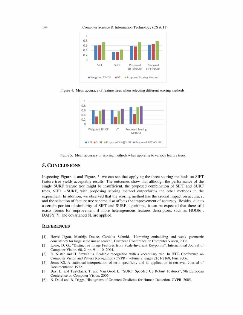
144 Computer Science & Information Technology (CS & IT)
Figure 4. Mean accuracy of feature trees when selecting different scoring methods.
Figure 5. Mean accuracy of scoring methods when applying to various feature trees.
5. CONCLUSIONS
Inspecting Figure. 4 and Figure. 5, we can see that applying the three scoring methods on SIFT
feature tree yields acceptable results. The outcomes show that although the performance of the
single SURF feature tree might be insufficient, the proposed combination of SIFT and SURF
trees, SIFT→SURF, with proposing scoring method outperforms the other methods in the
experiment. In addition, we observed that the scoring method has the crucial impact on accuracy,
and the selection of feature tree scheme also affects the improvement of accuracy. Besides, due to
a certain portion of similarity of SIFT and SURF algorithms, it can be expected that there still
exists rooms for improvement if more heterogeneous features descriptors, such as HOG[6],
DAISY[7], and covariance[8], are applied.
REFERENCES
[1] Hervé Jégou, Matthijs Douze, Cordelia Schmid. “Hamming embedding and weak geometric
consistency for large scale image search”, European Conference on Computer Vision, 2008.
[2] Lowe, D. G., “Distinctive Image Features from Scale-Invariant Keypoints”, International Journal of
Computer Vision, 60, 2, pp. 91-110, 2004.
[3] D. Nistér and H. Stewénius. Scalable recognition with a vocabulary tree. In IEEE Conference on
Computer Vision and Pattern Recognition (CVPR), volume 2, pages 2161-2168, June 2006.
[4] Jones KS, A statistical interpretation of term specificity and its application in retrieval. Journal of
Documentation,1972.
[5] Bay, H. and Tuytelaars, T. and Van Gool, L. “SURF: Speeded Up Robust Features”, 9th European
Conference on Computer Vision, 2006
[6] N. Dalal and B. Triggs. Histograms of Oriented Gradients for Human Detection. CVPR, 2005.
0
0.2
0.4
0.6
0.8
1
SIFT SURF Proposed
SIFT⊕SURF
Proposed
SIFT→SURF
Weighted TF-IDF VT Proposed Scoring Method
0
0.2
0.4
0.6
0.8
1
Weighted TF-IDF VT Proposed Scoring
Method
SIFT SURF Proposed Sift⊕SURF Proposed SIFT→SURF

Computer Science & Information Technology (CS & IT) 145
[7] Engin Tola, Vincent Lepetit, Pascal Fua. IEEE Transactions on Pattern Analysis and Machine
Intelligence. Vol. 32, Nr. 5, pp. 815 - 830, May 2010.
[8] Oncel Tuzel, Fatih Porikli, and Peter Meer, Pedestrian Detection via Classification on Riemannian
Manifolds, IEEE Transactions on Pattern Analysis and Machine Intelligence, Oct. 2008.

146 Computer Science & Information Technology (CS & IT)
INTENTIONAL BLANK

David C. Wyld et al. (Eds) : ITCS, CST, JSE, SIP, ARIA, DMS - 2015
pp. 147–155, 2015. © CS & IT-CSCP 2015 DOI : 10.5121/csit.2015.50115
THE CHAOTIC STRUCTURE OF
BACTERIAL VIRULENCE PROTEIN
SEQUENCES
Sevdanur Genc1, Murat Gok
2, Osman Hilmi Kocal
3
1Institute of Science, Yalova University, Yalova, Turkey
Department of Computer Engineering, Yalova University, Yalova, Turkey [email protected], [email protected]
ABSTRACT
Bacterial virulence proteins, which have been classified on structure of virulence, causes
several diseases. For instance, Adhesins play an important role in the host cells. They are
inserted DNA sequences for a variety of virulence properties. Several important methods
conducted for the prediction of bacterial virulence proteins for finding new drugs or vaccines.
In this study, we propose a method for feature selection about classification of bacterial
virulence protein. The features are constituted directly from the amino acid sequence of a given
protein. Amino acids form proteins, which are critical to life, and have many important
functions in living cells. They occurring with different physicochemical properties by a vector of
20 numerical values, and collected in AAIndex databases of known 544 indices.
For all that, this approach have two steps. Firstly, the amino acid sequence of a given protein
analysed with Lyapunov Exponents that they have a chaotic structure in accordance with the
chaos theory. After that, if the results show characterization over the complete distribution in
the phase space from the point of deterministic system, it means related protein will show a
chaotic structure.
Empirical results revealed that generated feature vectors give the best performance with chaotic
structure of physicochemical features of amino acids with Adhesins and non-Adhesins data sets.
KEYWORDS
Bioinformatics, Virulence Protein Sequences, Attribute Encoding, Chaotic Structure,
Classification.
1. INTRODUCTION
Proteins, which have vital importance for organisms, reacts in all biochemical reactions.
Physicochemical properties of amino acids are the most important determinant to formation for
three-dimensional structure of proteins and binding orders of amino acids. In addition,
physicochemical properties determine functions of proteins and life cycles.

148 Computer Science & Information Technology (CS & IT)
Physicochemical properties have different 544 input data. We think that these properties shows a
chaotic structure because they create a certain system and this certain system also affect
themselves.
According to chaos, a deterministic system can behave in irregular. In other words a deterministic
system can behave in an unexpected way. Chaos that depends on certain parameters usually
appear in undetermined, complicated and nonlinear systems.
544 physicochemical properties should be analyzed in a scalar form of data in the phase space by
regenerating. Equality of movements in phase space will show the results of the model to
quantiles such as positioning attractor dimensions and Lyapunox exponents of system.
Bacterial virulence protein sequences have similar patterns. On these similarities are pretty
difficult estimation for classification. In studies conducted to date, based on different strategies
about various methods have been proposed to estimation of virulence proteins. To illustrate, the
first studies and developed methods were based to search similarity such as BLAST [1] ve PSI-
BLAST [2]. In more recent times, machine learning algorithm used for estimation. In the recent
times, studied for estimation of bacterial virulence proteins about physicochemical properties.
Our aim in this study is that proving a chaotic structure of physicochemical properties of amino
acids that constitute bacterial virulence proteins.
2. MATERIALS AND METHODS
2.1 Dataset
In this study, Adhesins dataset has been used on SPAAN. Dataset have 469 Adhesins and 703
non-Adhesins proteins. Adhesins protein sequences were downloaded from http://www.ncbi.
nlm.nih.gov using the keyword 'Adhesin'. Non-adhesins, The rationale we used here was to
collect sequences of enzymes and other proteins that function within the cell. They probably have
remote possibility of functioning as adhesins and would differ in compositional characteristics
(Nakashima and Nishikawa, 1994) [3].
Also, current version of AAIndex included in the dataset. The AAIndex contains 544 amino acid
indices. For each the properties of 20 amino acids, input consists of reference information, a short
description of the index, an accession number and the numerical values.
In additional to this study, algorithm of this application developed on MatLab. For all Lyapunov
Exponents were calculated by Tisean Software.
2.2. Physicochemical Properties Of Amino Acids
Amino acids which, determine the functions of proteins have different physicochemical
properties such as hydrophobicity, polarity and molecular weight. These properties, termed the
amino acid indices, can be represented with 20 numeric values of vectors.
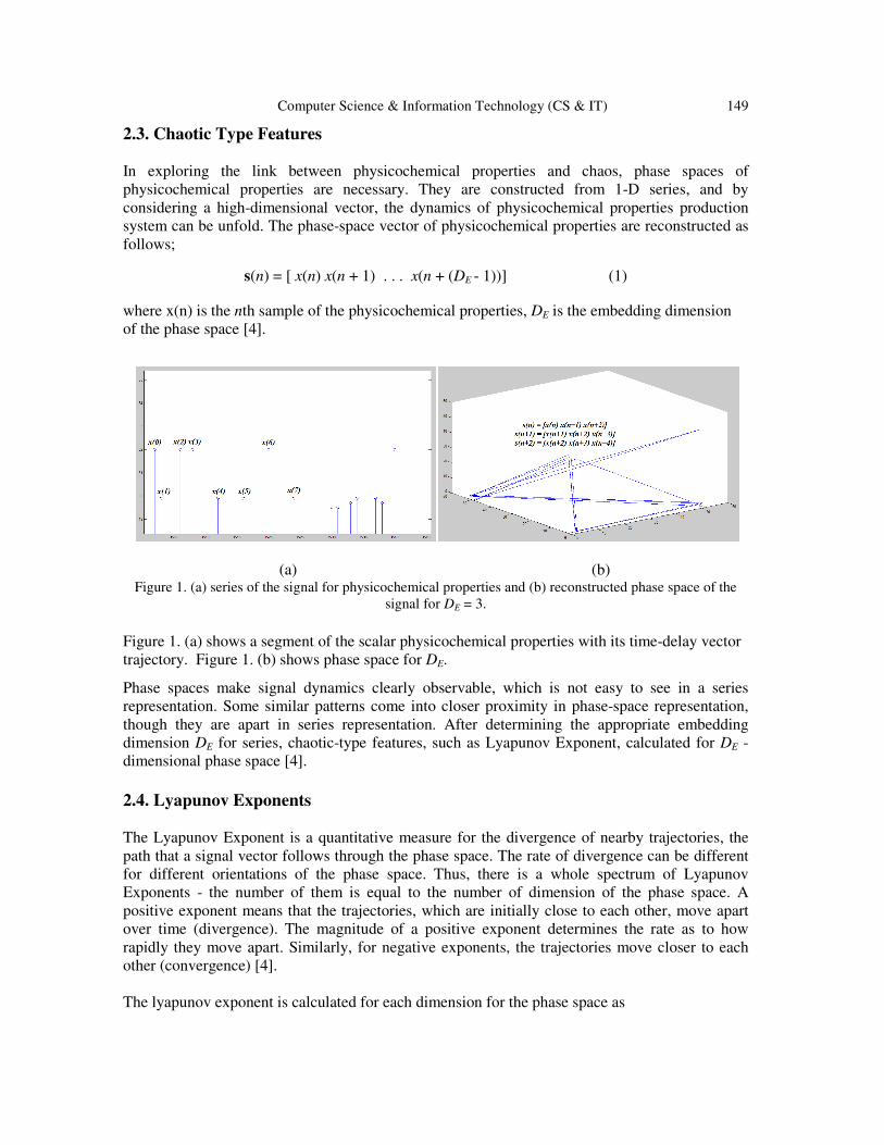
Computer Science & Information Technology (CS & IT) 149
2.3. Chaotic Type Features
In exploring the link between physicochemical properties and chaos, phase spaces of
physicochemical properties are necessary. They are constructed from 1-D series, and by
considering a high-dimensional vector, the dynamics of physicochemical properties production
system can be unfold. The phase-space vector of physicochemical properties are reconstructed as
follows;
s(n) = [ x(n) x(n + 1) . . . x(n + (DE - 1))] (1)
where x(n) is the nth sample of the physicochemical properties, DE is the embedding dimension
of the phase space [4].
(a) (b) Figure 1. (a) series of the signal for physicochemical properties and (b) reconstructed phase space of the
signal for DE = 3.
Figure 1. (a) shows a segment of the scalar physicochemical properties with its time-delay vector
trajectory. Figure 1. (b) shows phase space for DE.
Phase spaces make signal dynamics clearly observable, which is not easy to see in a series
representation. Some similar patterns come into closer proximity in phase-space representation,
though they are apart in series representation. After determining the appropriate embedding
dimension DE for series, chaotic-type features, such as Lyapunov Exponent, calculated for DE -
dimensional phase space [4].
2.4. Lyapunov Exponents
The Lyapunov Exponent is a quantitative measure for the divergence of nearby trajectories, the
path that a signal vector follows through the phase space. The rate of divergence can be different
for different orientations of the phase space. Thus, there is a whole spectrum of Lyapunov
Exponents - the number of them is equal to the number of dimension of the phase space. A
positive exponent means that the trajectories, which are initially close to each other, move apart
over time (divergence). The magnitude of a positive exponent determines the rate as to how
rapidly they move apart. Similarly, for negative exponents, the trajectories move closer to each
other (convergence) [4].
The lyapunov exponent is calculated for each dimension for the phase space as

150 Computer Science & Information Technology (CS & IT)
(2)
Here, s(n) is the reference point and s(m) is the nearest neighbor of s(n) on a nearby trajectory.
d(s(n),s(m)) is the initial distance between the nearest neighbors. d(s(n + 1),s(m + 1)) is the
distance between s(n + 1) and s(m + 1) which are the next pair of neighbors on their trajectories.
It must be considered that the LE calculation algorithm finds a new nearest neighbor s(m) for
each s(n), (n = 1,2,...,N). There are DE Lyapunov exponents (i.e., {λ1, λ2,..., λDE }) in descending
order. λ1 is known as the largest LE and a positive largest LE is the indicator of chaos [4].
After calculating lyapunov exponents for all of the nearest neighbor pairs on different trajectories,
the lyapunov exponent for the whole signal is calculated as the average of these lyapunov
exponents, as the magnitude on d(s(n),s(m)) depends on the whole phase space only, and
distortion does not change the global form of the phase space [4].
2.5. Tisean Software Project
In this study, developed of this project by Tisean. It is a software project for the analysis of time
series with methods based on the chaos theory. Tisean Package is analysis of time series with
methods based on the theory of nonlinear deterministic dynamical systems. Tisean software can
be downloaded from http://www.mpipks-dresden.mpg.de/~tisean/. Also, we studied with Cygwin
for Tisean software. Cygwin can be downloaded from https://www.cygwin.com/. In this problem,
using Tisean Package with MATLAB by Cygwin on Windows 7 operation system.
3. EXPERIMENTAL SETUP In this study, we advanced an algorithm that using Lyapunov exponents for the purpose of
classification using physicochemical properties of residues. Through this algorithm, we will
demonstrate chaotic structure of bacterial virulence protein sequences. We think that protein
sequences show chaotic structure with the physicochemical properties of amino acids. Our
hypothesis prove that, we developed an application which using Tisean Software Project with
MatLab. Figure 3. shows a work flow diagram forming of physicochemical properties.
According to Figure 2, first step, we used the AAIndex for values of 20 amino acids. AAIndex has
544 physicochemical properties to each amino acids. Thus, we have created a matrix with size of
[ 20 X 544 ]. Thereby, getting the length of each protein have created a matrix with size of [ 1 X
Protein Length ]. For example, show regard to protein that is hemolysin / hemagglutinin - like
protein HecA (Erwinia chrysanthemi). It consists by 3848 amino acid. So, This sequence should
be in size of 3848, and also should be create a matrix with size of [ 1 X 3848].
According to that matrix with size of [1 X 3848 ], can create a matrix with 544 physicochemical
properties for each amino acids about that proteins. So, length of the just created a matrix should
be in size of [ 544 X Protein Length ]. Also respectively created 544 files within terms of protein
length, line by line. And then, they saved and moved in one directory, called AA2File.

Computer Science & Information Technology (CS & IT) 151
Figure 2. Work Flow Diagram forming of physicochemical properties
The AA2File folder includes each files of 544 properties, in addition to that will be calculated all
of them with using Tisean Software Project by Matlab. And then, receive results of 544 properties
from Tisean. The file extensions named as .LYAP. Also, they saved and moved in one directory,
named as File2Lyap.
Whole of result are received by Tisean, because of that analyzed to convert at lyapunov exponent.
Lyapunov Exponents have observable results at LYAP file; such as protein length, signals belong
to each amino acids of a protein, average relative forecast erros, average absolute forecast errors,
average neighborhood size, average number of neighbors and estimated KY-Dimension. Last of
all, according to the signs of lyapunov exponents is given to the decision by Tisean.
Tabel 1. shows a lyapunov exponent results of the protein with 3848 length, as follows;
Table 1. The LEs results of the protein with 3848 length
The Lyapunov Exponents Results
Length of Protein (Amino Acid) : 3848
Signals belong to each amino acids of a protein :
9.044008e-001 4.018379e-001 2.226827e-001 1.310360e-001
4.904960e-002 -1.972889e-002 -1.013593e-001 -1.959663e-001
-3.338790e-001 -7.586726e-001
Average relative forecast errors : 1.157800e+000
Average absolute forecast errors : 2.145047e+001
Average Neighborhood Size : 2.398085e+001
Average num. of neighbors : 3.000000e+001
Estimated KY-Dimension : 10.000000

152 Computer Science & Information Technology (CS & IT)
Finally, LEs results show evidence of the better distribution by LYAP file, because of that the
chaos theory analyzed on 2-D or 3-D in phase space. Our results demonstrate that negative
lyapunov exponents and positive lyapunov exponents can be determined as quickly and easily,
simply by analyzing data in Tisean as Table 1. In such a case that, the first few positive and
negative exponents are enough to characterize the complete distribution. So, need to know for
sure that the chaotic system should to have at least one positive lyapunov exponents. According
to that this protein has five positive and five negative lyapunov exponents as Table1 shown. So,
there are more protein like this sample on Adhesins and non-Adhesins Datasets.
4. EXPERIMENTAL RESULTS
In this hypothesis, will explain with an experiment that fit for purpose with our algorithm. First of
all, shows physicochemical properties on phase space, after then calculate results of lyapunov
exponents. At the beginning that create a x vector by matrix size of [ 1 X 3848 ]. Figure 3. (a)
shows a line plot of the data values in x.
(a) (b)
Figure 3. (a) Creates a line plot of the data values in x and (b) shows a 2-D line plot of data.
nth sample of the physicochemical properties are calculated on 2-D phase space by MATLAB.
Thus, Figure 3. (b) shows a 2-D line plot of data, Y axis values and X axis values. And finally, nth
sample of the physicochemical properties are calculated on 3-D phase space by MATLAB. Thus,
Figure 4. shows X, Y and Z are vectors, plots one or more lines in three-dimensional space
through the points which coordinates are the elements of X, Y and Z.
Figure 4. Creates a 3-D line plot of the data values in X,Y and Z.

Computer Science & Information Technology (CS & IT) 153
In examined to Lyapunov Exponents signs, according to chaos has been shown an alteration on
the phase space, it may be appear or not. So, Lyapunov Exponent signs were vary chaotic
structure at phase space. Also, according to length of phase space that LEs show reconciliation
and rapprochement at all dimensions of LEs signs as Figure 4. shown. It has a real distribution on
phase space.
For this study, used Adhesins Dataset. Thus, give an example of the results, consider a protein
that is hemolysin / hemagglutinin - like protein HecA. Top of distributions' values have results
between greater or equal to 4. For instance, these values generally have four positive and six
negative signs, five positive and five negative signs, six positive and four negative signs etc.
If analyze the Table 2., show the best results from 544 properties on AAIndex Table via Tisean -
Lyapunov Exponent Calculator.
Table 2. Gives the best results for protein HecA
Featues of AAIndex Positive Negative
14 4 6
96 4 6
114 4 6
173 4 6
185 4 6
247 4 6
252 4 6
400 5 5
488 4 6
496 4 6
537 4 6
538 4 6
539 4 6
543 4 6
If analyze the Table 3., shown Lyapunov Exponents, that include to five postive and five negative
on phase space, according to chaos theory has distribution as chaotic structure.
Table 3. Lyapunov Exponents belong to each aminoacids for protein HecA
LEs belong to each aminoacids of protein HecA
Positive Negative
9.044008e-001 -1.972889e-002
4.018379e-001 -1.013593e-001
2.226827e-001 -1.959663e-001
1.310360e-001 -3.338790e-001
4.904960e-002 -7.586726e-001
Consequently, we have proved this hypothesis that physicochemical properties have distribution
on phase space as chaotic structure. So, there are positive and negative signs from lyapunov

154 Computer Science & Information Technology (CS & IT)
exponents of phase space at this distribution, and in addition that belong to each amino acids of
proteins on Adhesins dataset.
5. RESULTS In this paper, we analyzed to Adhesins and non-Adhesins datasets at chaotic structure at phase
space. Shortly after, we determined the best physicochemical features on these dataset by result of
Lyapunov Exponents. Therefore, if analyzed to other datasets on phase space, in our opinion that
dataset will obtain different results about physico chemical features. In the future works, we will
be using our developed method, also will be improving this algorithm for classification to
unfolded protein regions.
Unfolded protein regions plays an important role in determining transcriptional and translational
regulation of the protein, protein-protein, protein-DNA interactions and tertiary structure. To date,
studies have been shown that unfolded regions associated with cancer, cardiovascular, diabetes,
autoimmune diseases and neurodegenerative disorders.
As a result, will be explained to generate feature vectors that using with chaotic structure for
prediction of unfolded protein regions and also we will be making comparison with similar
studies in the literature about classification and recognition.
ACKNOWLEDGEMENTS This work was performed with aim of master thesis under the auspices of the Department of
Computer Engineering under The University of Yalova.
REFERENCES
[1] S.F. Altschul, W. Gish, W. Miller, E.W. Myers, and D.J. Lipman, “Basic Local Alignment Search
Tool”, J. Molecular Biology, vol. 215, pp. 403-410, 1990
[2] S.F. Altschul, T.L. Madden, A.A. Schaffer, J. Zhang, Z. Zhang, W. Miller, and D.J. Lipman, “Gapped
BLAST and PSI-BLAST: A New Generation of Protein Database Search Programs”, Nucleic Acids
Research, vol. 25, pp. 3389-3402, 1997.
[3] Sachdeva, G., Kumar, K., Jain, P., and Ramachandran, S. "SPAAN: a software program for prediction
of adhesins and adhesin-like proteins using neural networks", Bioinformatics, vol. 21, pp. 483-491,
2005.
[4] Kocal, O.H., Yuruklu, E., Avcibas, I. "Chaotic-Type Features for speech steganalysis", IEEE
Transactions on Information Forensics and Security, vol. 3, pp. 651-661, 2008a
Computer Science & Information Technology (CS & IT) 155
AUTHORS
Osman Hilmi Kocal was born in Istanbul, Turkey, in 1967. He received the B.Sc., M.Sc.,
and Ph.D. degrees in electronics and telecommunication engineering from the Technical
University of Istanbul, Istanbul, in 1989, 1992, and 1998, respectively. He was a Research
Assistant with the Technical University of Istanbul and Turkish Air Force Academy,
Istanbul, respectively. Currently, he is an Assistant Professor with the Department of
Computer Engineering, Yalova University, Yalova, Turkey. His research interests include
chaotic signals and adaptive signal processing.
Murat Gok was born in Kirsehir, Turkey in 1976. He received the B.Sc. degree in
electrical and computer education from the Marmara University, Istanbul, in 2000. The
M.Sc. degree in electrical and computer education from the Mugla University, Mugla, in
2006. And the Ph.D. degree in electrical and computer education from the Sakarya
University, Sakarya, in 2011. Currently, he is an Assistant Professor with the Department
of Computer Engineering, Yalova University, Yalova, Turkey. His research interests
include pattern recognition, machine learning algorithms, feature extraction and selection, bioinformatics,
protein classification and decision support systems.
Sevdanur Genc was born in Istanbul, Turkey in 1983. She received the B.Sc. degree in
computer engineering from the Suleyman Demirel University, Isparta, 2010. Also, She is
currently pursuing the M.Sc. degree in computer engineering from the Yalova University,
Yalova. Her research interests include cloud computing, parallel programming,
bioinformatics, remote sensing, machine learning algorithms, computer vision and pattern
recognition.

156 Computer Science & Information Technology (CS & IT)
INTENTIONAL BLANK

David C. Wyld et al. (Eds) : ITCS, CST, JSE, SIP, ARIA, DMS - 2015
pp. 157–164, 2015. © CS & IT-CSCP 2015 DOI : 10.5121/csit.2015.50116
ANT COLONY OPTIMIZATION FOR
CAPACITY PROBLEMS
Tad Gonsalves and TakafumiShiozaki
Department of Information and Communication Sciences,
Faculty of Science & Technology, Sophia University, Tokyo, Japan [email protected], [email protected]
ABSTRACT
This paper deals with the optimization of the capacity of a terminal railway station using the
Ant Colony Optimization algorithm. The capacity of the terminal station is defined as the
number of trains that depart from the station in unit interval of time. The railway capacity
optimization problem is framed as a typical symmetrical Travelling Salesman Problem (TSP),
with the TSP nodes representing the train arrival /departure events and the TSP total cost
representing the total time-interval of the schedule. The application problem is then optimized
using the ACO algorithm. The simulation experiments validate the formulation of the railway
capacity problem as a TSP and the ACO algorithm produces optimal solutions superior to those
produced by the domain experts.
KEYWORDS
Travelling Salesman Problem, Ant Colony Optimization, Capacity Problems, Meta-heuristic
Optimization, Soft Computing.
1. INTRODUCTION
This study focuses on the simulation optimization of rail capacity, a prominent application
problem in the transportation domain. Zhu [1] defines the railway capacity as the maximum
number or pair of trains with standard load passing by a fixed equipment in unit time (usually one
day) on the basis of the given type of locomotives and vehicles. It usually depends on the
condition of the fixed equipment as well as the organization of the train operation. According to
the European Community directives [2], the provision, maintenance and marketing of the railway
track capacities should be separated from the operation of trains. This would imply a separation
of the management of the railway infrastructure from the management of the railway operation.
With this in mind, we frame the aim of this study as: the optimization of rail capacity by
managing the train operation, given a fixed railway network and equipment infrastructure. In
particular, we focus on the capacity of a terminal station, i.e., the number of trains departing from
the terminal station in unit time. The problem basically boils down to constructing an optimal
schedule of the passenger trains so as to maximize the terminal station capacity. However, owing
to the multiple decision variables, the problem becomes a typical combinatorial optimization
problem which cannot be solved using the conventional optimization algorithms.

158 Computer Science & Information Technology (CS & IT)
In order to solve the combinatorial optimization problem, we first cast it in the form of a
Travelling Salesman Problem and use some of the soft–computing techniques to find the optimal
solution. Although the TSP has applications in practical problems like Vehicle Routing, Job
Sequencing, Computer Wiring, etc. [3], it is known to be NP hard. Since brute force approach is
an infeasible option, heuristics approach can be fairly relied upon to solve thesetypes of problems
since heuristics approach utilizes much less computing power. Some of the conventional heuristic
techniques designed to solve the TSP include branch and cut [4], dynamic programming [5],
regression analysis [6], exact methods [7], etc. Recently many meta-heuristic algorithms (i.e.
heuristics that do not depend on the domain knowledge of the problem) are successfully
employed to search for the optimal TSP solution. The Genetic Algorithm (GA) based on the
Darwinian theory of natural selection and its variants are reported to be successful in finding the
optimal solutions to the benchmark TSP problems in a reasonable amount of computing time [8-
11]. In some studies, the Genetic Algorithm is combined with other meta-heuristic optimization
algorithms to improve the optimization results [12].
However, the most successful soft computing algorithm to obtain the optimal solution of the TSP
is the Ant Colony Optimization (ACO) algorithm. The development of the ACO algorithm has
been inspired by the foraging behaviour of some ant species. These ants deposit pheromone on
the ground in order to mark some favourable path that should be followed by other members of
the colony. The ACO algorithm exploits a similar mechanism for solving optimization problems
[13-19]. From the early nineties, when the first ACO algorithm was proposed, it has attracted the
attention of an increasing numbers of researchers and it has been extended to many successful
applications.
In this study, the railway capacity optimization problem is cast in the form of a TSP. The
arrival/departure events in the schedule are treated as nodes which need to be ordered under the
given scheduling constraints so as to minimize the entire schedule time. Some of the other
constraints are imposed by the track-changing hardware equipment. The time between two events
is considered to be the distance between two TSP edges and the train operation schedule is
considered to be the tour length of the TSP. The standard ACO application to this problem yields
an optimal schedule, under the given infrastructure and operational constraints.
This paper is organized as follows: Section 2 describes the TSP and ACO. Section 3 describes the
formulation of the railway capacity optimization problem (RCP) as the TSP and its solution using
the standard ACO algorithm. Section 4 presents the simulation optimization results and section 5
concludes the paper.
2. TSP AND ACO
In this section, we introduce the Travelling Salesman Problem and the Ant Colony Optimization
algorithm. We show how the Ant Colony Optimization algorithm is designed to solve the
Travelling Salesman Problem.
2.1. Travelling Salesman Problem (TSP)
The Travelling Salesman Problem (TSP) is a classic problem in computer science which may be
stated as follows: Given a list of cities and their pairwise distances, the task is to find the
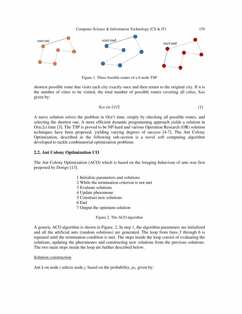
Computer Science & Information Technology (CS & IT) 159
Figure 1. Three feasible routes of a 6-node TSP
shortest possible route that visits each city exactly once and then return to the original city. If n is
the number of cities to be visited, the total number of possible routes covering all cities, Snis
given by:
Sn= (n-1)!/2 (1)
A naive solution solves the problem in O(n!) time, simply by checking all possible routes, and
selecting the shortest one. A more efficient dynamic programming approach yields a solution in
O(n22n) time [3]. The TSP is proved to be NP-hard and various Operation Research (OR) solution
techniques have been proposed, yielding varying degrees of success [4-7]. The Ant Colony
Optimization, described in the following sub-section is a novel soft computing algorithm
developed to tackle combinatorial optimization problems.
2.2. Ant Colony Optimization CO
The Ant Colony Optimization (ACO) which is based on the foraging behaviour of ants was first
proposed by Dorigo [13].
1 Initialize parameters and solutions
2 While the termination criterion is not met
3 Evaluate solutions
4 Update pheromone
5 Construct new solutions
6 End
7 Output the optimum solution
Figure 2. The ACO algorithm
A generic ACO algorithm is shown in Figure. 2. In step 1, the algorithm parameters are initialized
and all the artificial ants (random solutions) are generated. The loop from lines 2 through 6 is
repeated until the termination condition is met. The steps inside the loop consist of evaluating the
solutions, updating the pheromones and constructing new solutions from the previous solutions.
The two main steps inside the loop are further described below.
Solution construction
Ant k on node i selects node j, based on the probability, pij, given by:

160 Computer Science & Information Technology (CS & IT)
where denotes the set of candidate sub-solutions; τij and ηij denote, respectively, the pheromone
value and the heuristic value associated with eij.
Updating the pheromone
The pheromone update operator employed for updating the pheromone value of each edge eijis
defined as
Where Lkdenotes the quality of the solution created by ant k; denotes the evaporation
rate.
3. CAPACITY PROBLEM AS TSP
This section describes in detail the railway capacity problem to be optimized. It explains the
optimization constraints, the framing of the railway capacity problem as a typical TSP and finally
the solution process by using the standard ACO algorithm.
3.1. Capacity Problem
When dealing with the railway capacity problem, the railway management has to consider the
different types of capacities in the railway domain. Some of the relevant capacities, for instance,
are: (1) the capacity of the platform to hold passengers, (2) the capacity of the carriages to hold
passengers, (3) the rail network capacity to hold the number of trains at a given time, and (4) the
capacity of the railway station structure to schedule the maximum number of trains per unit time.
Dealing with all these types of capacities simultaneously is a complex problem. This study is
dedicated to the maximization of only the type 4 railway capacity, i.e., maximization of the
number of trains that can be scheduled at a railway station per unit time. The type 4 rail capacity
optimization in turn leads to optimization of the royalties and alleviation of the congestion
problem during rush hours.
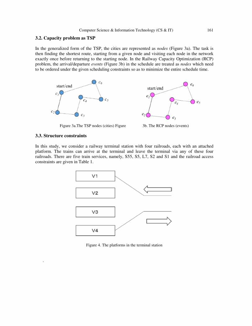
Computer Science & Information Technology (CS & IT) 161
3.2. Capacity problem as TSP
In the generalized form of the TSP, the cities are represented as nodes (Figure 3a). The task is
then finding the shortest route, starting from a given node and visiting each node in the network
exactly once before returning to the starting node. In the Railway Capacity Optimization (RCP)
problem, the arrival/departure events (Figure 3b) in the schedule are treated as nodes which need
to be ordered under the given scheduling constraints so as to minimize the entire schedule time.
Figure 3a.The TSP nodes (cities) Figure 3b. The RCP nodes (events)
3.3. Structure constraints
In this study, we consider a railway terminal station with four railroads, each with an attached
platform. The trains can arrive at the terminal and leave the terminal via any of these four
railroads. There are five train services, namely, S55, S5, L7, S2 and S1 and the railroad access
constraints are given in Table 1.
Figure 4. The platforms in the terminal station
.

162 Computer Science & Information Technology (CS & IT)
Table 1. Given parameters of the train capacity problem
4. OPTIMIZATION RESULTS
The aim of the simulation experiments using the ACO algorithm is to maximize the number of
trains leaving the terminal station in an hour. However, to reduce the calculation load, we divide
the hourly interval into 5 equal intervals, each being of 720 seconds (12 minutes) duration. The
assumption here is that the train schedule is periodic. The same period can then be stretched over
an hour. In Table 3, the final capacity of the terminal station is calculated by using the following
formula:
where, T is the total time for the entire schedule covering a period of 720 seconds.
The minimum time for the entire schedule over a period of 720 seconds is found to be 555
seconds and correspondingly the maximum capacity is 38.9 trains/hour
We conducted several experiments by varying the and parameters of the ACO algorithm.
Some of the optimal results obtained by these tuned parameters are shown in Table 4. Another
important parameter that needs an empirical tuning is the population size of the agents, N. Table 5
shows the results obtained by varying this number. As expected, the larger the population size,
the better the results are, although this increases the computational overhead.
Table 2. Varying the population size of the ACO agents
Computer Science & Information Technology (CS & IT) 163
5. CONCLUSIONS
The Ant Colony Optimization soft computing algorithm is apt for solving combinatorial
optimization problems like the classical NP-hard Travelling Salesman Problem. Basing the search
on the stigmery of the food foraging real-life ant colony, the algorithm explores the huge search
space of the NP-hard problems to find the optimal solution. In this study, the authors have applied
the ACO algorithm to optimize the capacity of a terminal railway station. The capacity
optimization problem is cast into the form of a TSP-like problem, where the arrival and departure
events of the trains are considered to be the nodes and the schedule length as the TSP total route.
The standard ACO optimizes the schedule length subject to the infrastructure and operational
constraints. The simulation experiments validate the formulation of the railway capacity problem
as a TSP. The optimal solutions obtained by the soft-computing technique is superior to those
produced by the domain experts.
REFERENCES
[1] Xiaoning Zhu, “Computer-based simulation analysis of railway carrying capacity utilization”,
Proceedings of the International Conferences on Info-tech and Info-net, ICII2001, Beijing, 2001,
vol.4, pp.107-112.
[2] Kuckelberg, A., “Component based system architecture for railway capacity management systems”,
Proceedings of the Fourth International Conference on Quality Software, QSIC 2004., pp.189-196.
[3] Rajesh Matai, Surya Singh and Murari Lai Mittal (2010). Traveling Salesman Problem: an Overview
of Applications, Formulations, and Solution Approaches, Traveling Salesman Problem, Theory and
Applications, Donald Davendra (Ed.), pp. 1-24.
[4] Sarubbi, J.; Miranda, G.; Luna, H.P.; Mateus, G., “A Cut-and-Branch algorithm for the
Multicommodity Traveling Salesman Problem,” IEEE International Conference on ,Service
Operations and Logistics, and Informatics, IEEE/SOLI 2008, vol.2, pp.1806-1811.
[5] Jellouli, O., “Intelligent dynamic programming for the generalised travelling salesman problem,”
2001, IEEE International Conference on Systems, Man, and Cybernetics, 2001, vol.4, pp.2765-2768.
[6] Shut, V., Prozherin, I., “A solution of travelling salesman problem by a method of correlative-
regression analysis,” Intelligent Data Acquisition and Advanced Computing Systems: Technology
and Applications, International Workshop on, 2001, pp.267-269.
[7] Woeginger, G.J. (2003), “Exact Algorithms for NP-Hard Problems: A Survey”, Combinatorial
Optimization – Eureka, You Shrink! Lecture notes in computer science, vol. 2570, Springer, pp. 185–
207.
[8] Pullan, W., “Adapting the genetic algorithm to the travelling salesman problem,” The 2003 Congress
on Evolutionary Computation, CEC '03, 2003, vol.2, pp.1029-1035.
[9] FatihTasgetiren, M.; Suganthan, P.N.; Quan-ke Pan; Yun-Chia Liang, “A genetic algorithm for the
generalized traveling salesman problem,” IEEE Congress on Evolutionary Computation, CEC 2007,
2007, pp.2382-2389.
[10] Geetha, R.R., Bouvanasilan, N., Seenuvasan, V., “A perspective view on Travelling Salesman
Problem using genetic algorithm,” World Congress on Nature & Biologically Inspired Computing,
NaBIC 2009, 2009, pp.356-361.
[11] Mudaliar, D.N., Modi, N.K., “Unraveling Travelling Salesman Problem by genetic algorithm using
m-crossover operator,” International Conference on Signal Processing Image Processing & Pattern
Recognition (ICSIPR), 2013, pp.127-130.
[12] Chen, S.M., &Chien, C.Y. (2011). Solving the traveling salesman problem based on the genetic
simulated annealing ant colony system with particle swarm optimization techniques. Expert Systems
with Applications, vol. 38, pp. 14439-14450.
[13] Dorigo, M. (1992). Optimization, learning and natural algorithms.Politecnico di Milano, Italy: Ph.D.
Thesis.

164 Computer Science & Information Technology (CS & IT)
[14] Dorigo, M., & Caro, D. G. (1999). Ant colony optimization: a new meta-heuristic (vol. 2). Proceeding
of the 1999 Congress on Evolutionary Computation.
[15] Dorigo, M., Maniezzo, V., &Colorni, A. (1996). Any System: Optimization by a colony of
cooperating agents. IEEE Trans Syst Man Cybernet Part B.
[16] Doringo, M., & Gambardella, L. M. (1997). A cooperative learninig approach to the traveling
salesman problem.IEEE Transactions on Evolutionary Computation.
[17] Bullnheimer, B., Hartl, R., & Strauss, C. (1999). A new rank-based version of the Ant System: A
computational study. Central European J Operations Res Econom.
[18] Blum, C., &Dorigo, M. (2004). The hyper-cube framework for ant colony optimization. IEEE Trans
Syst Man Cybernet Part B, 34(2), 1161-1172.
[19] M. Dorigo and T. Stützle.Ant Colony Optimization.MIT Press, Cambridge, MA, 2004.
AUTHORS
Dr. Tad Gonsalvesobtained the BS degree in theoretical Physics and the MS degree in Astrophysics from
the Pune University. He obtained the PhD in Systems Engineering from Sophia University, Tokyo, Japan.
Currently he is an Assistant Professor in the Department of Information and Communication Sciences,
Faculty of Science & Technology in the same university. His research interests include design of Expert
Systems, Evolutionary Algorithms, Machine Learning and Parallel Programming.
TakafumiShiozakiis an under-graduate student is the Department of Information and Communication
Sciences, Faculty of Science & Technology, Sophia University, Tokyo, Japan. His research is on the
application of the Evolutionary Algorithms to diverse real-world problems.
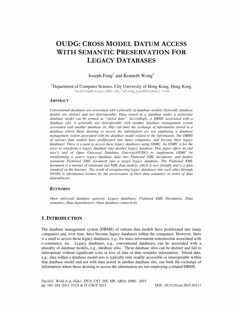
David C. Wyld et al. (Eds) : ITCS, CST, JSE, SIP, ARIA, DMS - 2015
pp. 165–184, 2015. © CS & IT-CSCP 2015 DOI : 10.5121/csit.2015.50117
OUDG: CROSS MODEL DATUM ACCESS
WITH SEMANTIC PRESERVATION FOR
LEGACY DATABASES
Joseph Fong
1 and Kenneth Wong
2
1Department of Computer Science, City University of Hong Kong, Hong Kong
[email protected],[email protected]
ABSTRACT Conventional databases are associated with a plurality of database models. Generally database
models are distinct and not interoperable. Data stored in a database under a particular
database model can be termed as “siloed data”. Accordingly, a DBMS associated with a
database silo, is generally not interoperable with another database management system
associated with another database sil. This can limit the exchange of information stored in a
database where those desiring to access the information are not employing a database
management system associated with the database model related to the information. The DBMS
of various data models have proliferated into many companies, and become their legacy
databases. There is a need to access these legacy databases using ODBC. An ODBC is for the
users to transform a legacy database into another legacy database. This paper offers an end
user’s tool of Open Universal Database Gateway(OUDG) to supplement ODBC by
transforming a source legacy database data into Flattened XML documents, and further
transform Flattened XML document into a target legacy database. The Flattened XML
document is a mixture of relational and XML data models, which is user friendly and is a data
standard on the Internet. The result of reengineering legacy databases into each other through
OUDG is information lossless by the preservation of their data semantics in terms of data
dependencies.
KEYWORDS
Open universal database gateway, Legacy databases, Flattened XML Documents, Data
semantics, Data dependencies, Open database connectivity
1. INTRODUCTION
The database management system (DBMS) of various data models have proliferated into many
companies and, over time, have become legacy databases within the companies. However, there
is a need to access these legacy databases, e.g., for mass information transmission associated with
e-commerce, etc. Legacy databases, e.g., conventional databases, can be associated with a
plurality of database models, e.g., database silos. These database silos can be distinct and fail to
interoperate without significant costs or loss of data or data semantic information. Siloed data,
e.g., data within a database model acts is typically only readily accessible or interoperable within
that database model and not with data stored in another database silo, can limit the exchange of
information where those desiring to access the information are not employing a related DBMS.

166 Computer Science & Information Technology (CS & IT)
Additionally, even where a database environment is relatively modern, it can be incompatible
with other relatively modern database silos. The plurality of database silos in itself can be an
impediment to sharing data among them. As an example, where a first company employs a first
database associated with a first database model, a second company employs a second data model
for their data, and a third company employs a third data model for their data, sharing of data
across the three data silos can be impractical or impossible. Where the first company purchase
the second company, incorporating the second company’s data can be problematic, e.g., it can
require rewriting the data into the first data model at the risk of losing data or semantics.
Alternatively, the first company can operate the two databases separately but are then internally
faced with the incongruences of the two databases, bear the costs associated with operating or
maintaining two separate databases, etc. Further, the first company, even with access to the first
and second databases, still can face serious challenges with sharing data with the third company.
The evolution of database technologies intend to meet different users requirements. For example,
the Hierarchical and Network (Codasyl) databases(NDB) are good for business computing on the
large mainframe computers. The user friendly relational databases(RDB) are good for end user
computing on personal computers. The object‐oriented databases(OODB) are good for
multi‐media computing on mini computers. The XML databases(XML DB) are good for Internet
computing on the mobile devices. These are first generation Hierarchical and Network databases,
second generation relational databases, and third generation Object-Oriented and XML databases.
Flattened XML documents
Flattened XML documents are generic representation of any legacy database instance in any
legacy database data model. Flattened XML document is a valid XML document which contains
a collection of elements of various types and each element defines its own set of properties. The
structure of the flattened XML document data file is a relational table structured XML document.
It has XML document syntax with relational table structure. It replaces primary key with ID, and
foreign key with IDREF as follows:
<?xml version="1.0">
<root>
<table1 ID="…" IDREF1="…" IDREF2="…" … IDREFN="…">
<attribute1>…</attribute1>
…
<attributeN>…</attributeN>
</table1>
…
<tableN ID="…" IDREF1="…" IDREF2="…" … IDREFN="…">
<attribute1>…</attribute1>
…
<attributeN>…</attributeN>
</tableN>
</root>
For each table, the name of the table (tableN) determines its type name and the name of property
(attributeN) determines its property name. Each table defines an ID type attribute that can
uniquely identify itself and there are optional multiple IDREF type attributes that can refer to the
ID in other tables in the same flattened XML document instance. Each property XML element
encloses a property value in a proper textual representation format. In order to ensure a flattened
XML document instance to be valid, there must be either an internal or an external DTD
document that defines the XML structures and attribute types, in particular for those ID and
IDREF type attributes.

Computer Science & Information Technology (CS & IT) 167
Open Universal Database Gateway
An open universal database gateway(OUDG) is a database middleware which provides more
flexibility for the users to access legacy databases in their own chosen data model. Users can
apply OUDG to transform legacy databases into flattened XML documents, and then further
transform them into user’s own familiar legacy database for access. Since XML is the data
standard on the Internet, it becomes information highway for user to access data.
The reason we choose flattened XML document is due to its openness for DBMS independence.
All other data models are DBMS dependent. For example, an Oracle database can only be
accessed by Oracle DBMS, and a MS SQL Server database can only be accessed by MS SQL
Server DBMS. Nevertheless, users can access flattened XML documents on the Internet by
Internet Explorer without programming. Therefore, an Oracle user can access an MS SQL Server
database by using OUDG transforming the MS SQL Server database into flattened XML
document, and then further transform flattened XML document to Oracle database.
Similarly, the reason we choose relational table structure for the flattened XML document is that
relational table structure has a strong mathematical foundation of relational algebra to implement
the constraints of major data semantics such as cardinality, isa and generalization to meet users’
data requirements by replacing primary keys and foreign keys into ID(s) and IDREF(s) in XML
schema.
The OUDG can transform legacy databases into flattened XML document, and then further
transform the flattened XML document into one of four target legacy databases: relational,
object-oriented, XML and network. The result is that OUDG allows users reengineer a source
legacy database into an equivalent target legacy database of user’s choice with data semantics
preservation.
This paper offers flattened XML documents as universal database medium for the interoperability
of all legacy databases that can be accessed by the users using their own familiar legacy database
language via OUDG. We consider hierarchical data model same as XML data model in this paper
because they are all in tree structure. All proprietary legacy data models can be united into
flattened XML document as universal database as shown in Figure 1.
Figure 1. Legacy Databases Interoperability via Flattened XML documents
The major difference between regular tree-based XML document and flattened XML document is
that the latter is more user friendly and efficient in database update since its database navigation
access path is much shorter than the former. The flattened XML document database navigation
access path is limited to 2 levels from root element to sibling elements while the regular XML
document database access path is in several levels and much longer in general.

168 Computer Science & Information Technology (CS & IT)
Problems:
(1) Most legacy database systems are proprietary. Database vendors do not facilitate tools to
export their databases to other legacy databases. Thus, companies need to use ODBC to access
heterogeneous databases, which requires programming and much time effort.
(2) Most users cannot access all legacy databases because they do not know all legacy database
languages. They rely on ODBC, which is not easy to learn.
(3) It is difficult to convert legacy databases in different data models because the data conversion
of legacy database involves data models transformation.
Solution:
Through OUDG, users can use one database language access another legacy databases of
relational, object-oriented, network and XML. The operation is more reliable and speedy because
same data can be concurrently processed by legacy database and their equivalent flattened XML
document.
Academic merit:
The novelty is that it is feasible to replace ODBC by OUDG transforming legacy database into
flattened XML document for access. ODBC needs programming, but OUDG is an end user
software utility.
Industrial merit:
The application of flattened XML document is for information highway on the Internet for data
warehouse, decision support systems (Fong, Li & Huang, 2003). The benefits are information
sharing among users for database interoperability.
OUDG as supplement for ODBC
OUDG can supplement ODBC to access any legacy database by transforming(reengineering)
them into a flattened XML document for access as universal database which is defined as a
database interchangeable to all legacy databases.
At present, most database systems are proprietary. Each DBMS vendor has software tools which
convert other legacy databases into databases using their own DBMS(s), but not vice versa for
converting their own databases into a target legacy database. The result makes legacy databases
not open to each other. However, using OUDG, any legacy database can be transformed into any
other legacy database via flattened XML documents. The benefit is that data sharing and data
conversion among legacy databases becomes possible. The openness of legacy database is
necessary for such application such as data warehousing, data mining and big data.
Figure 2 shows the architecture of an open universal database gateway which transforms legacy
databases into each other with different data models via flattened XML document as a
replacement for open database connectivity.
Data Semantics preservation in legacy databases
Data semantics describe data definitions and data application for users’ data requirements, which
can be captured in the database conceptual schemas. The following are the data semantics which
can be preserved among the legacy conceptual schemas and their equivalent flattened XML
schema:
(a) Cardinality: 1:1, 1:n and m:n relationships set between two classes
A one-to-one relationship between set A and set B is defined as: For all a in A, there exists at
most one b in B such that a and b are related, and vice versa. The implementation of one-to-one
relationship is similar to one-to-many relationship.
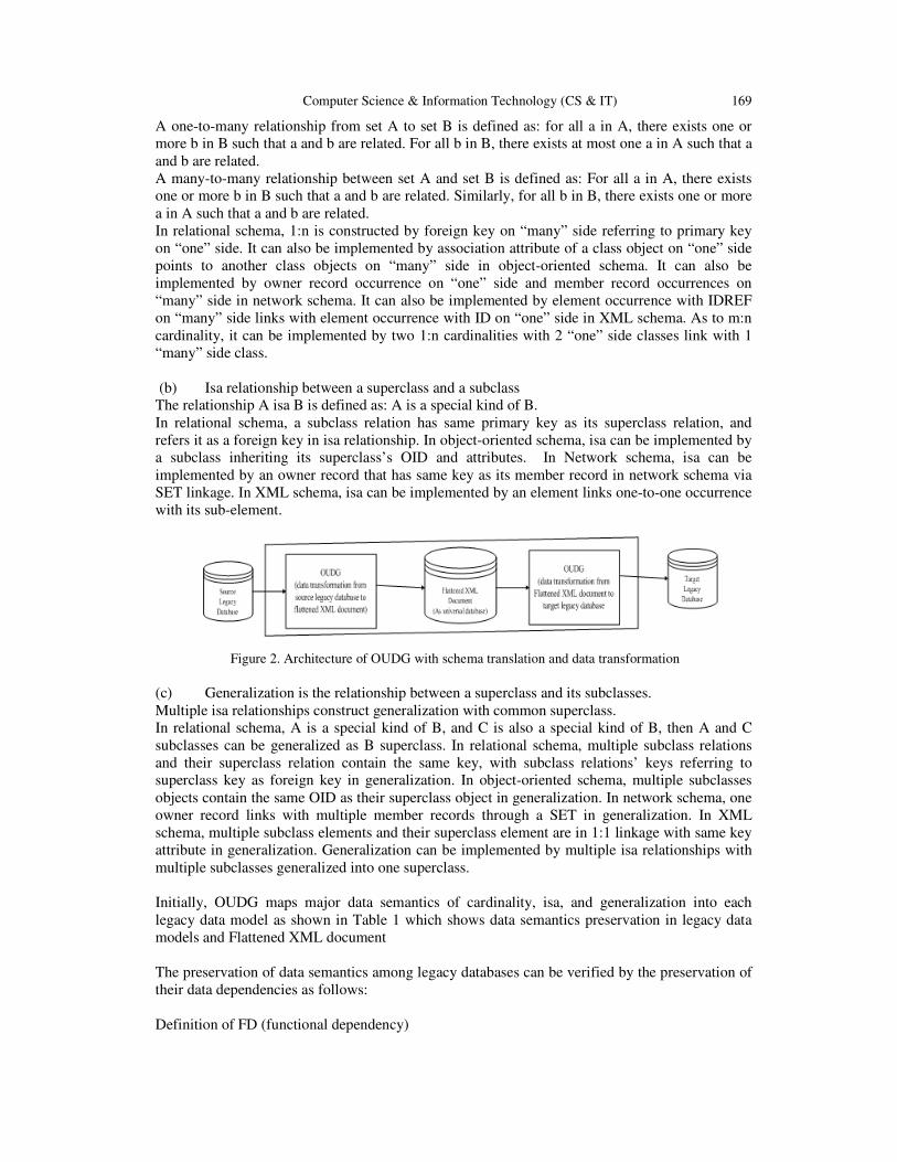
Computer Science & Information Technology (CS & IT) 169
A one-to-many relationship from set A to set B is defined as: for all a in A, there exists one or
more b in B such that a and b are related. For all b in B, there exists at most one a in A such that a
and b are related.
A many-to-many relationship between set A and set B is defined as: For all a in A, there exists
one or more b in B such that a and b are related. Similarly, for all b in B, there exists one or more
a in A such that a and b are related.
In relational schema, 1:n is constructed by foreign key on “many” side referring to primary key
on “one” side. It can also be implemented by association attribute of a class object on “one” side
points to another class objects on “many” side in object-oriented schema. It can also be
implemented by owner record occurrence on “one” side and member record occurrences on
“many” side in network schema. It can also be implemented by element occurrence with IDREF
on “many” side links with element occurrence with ID on “one” side in XML schema. As to m:n
cardinality, it can be implemented by two 1:n cardinalities with 2 “one” side classes link with 1
“many” side class.
(b) Isa relationship between a superclass and a subclass
The relationship A isa B is defined as: A is a special kind of B.
In relational schema, a subclass relation has same primary key as its superclass relation, and
refers it as a foreign key in isa relationship. In object-oriented schema, isa can be implemented by
a subclass inheriting its superclass’s OID and attributes. In Network schema, isa can be
implemented by an owner record that has same key as its member record in network schema via
SET linkage. In XML schema, isa can be implemented by an element links one-to-one occurrence
with its sub-element.
Figure 2. Architecture of OUDG with schema translation and data transformation
(c) Generalization is the relationship between a superclass and its subclasses.
Multiple isa relationships construct generalization with common superclass.
In relational schema, A is a special kind of B, and C is also a special kind of B, then A and C
subclasses can be generalized as B superclass. In relational schema, multiple subclass relations
and their superclass relation contain the same key, with subclass relations’ keys referring to
superclass key as foreign key in generalization. In object-oriented schema, multiple subclasses
objects contain the same OID as their superclass object in generalization. In network schema, one
owner record links with multiple member records through a SET in generalization. In XML
schema, multiple subclass elements and their superclass element are in 1:1 linkage with same key
attribute in generalization. Generalization can be implemented by multiple isa relationships with
multiple subclasses generalized into one superclass.
Initially, OUDG maps major data semantics of cardinality, isa, and generalization into each
legacy data model as shown in Table 1 which shows data semantics preservation in legacy data
models and Flattened XML document
The preservation of data semantics among legacy databases can be verified by the preservation of
their data dependencies as follows:
Definition of FD (functional dependency)

170 Computer Science & Information Technology (CS & IT)
Given a relation R, attribute Y of R is functionally dependent on attribute X of R, i.e., FD: R.X �
R.Y, iff each X-value in R has associated with it precisely one Y value in R. Attribute X and Y
may be composite.
Definition of ID (inclusion dependency)
ID: Y Z states that the set of values appearing in attribute Y must be a subset of the set of
values appearing in attribute Z.
Definition of MVD (multi-valued dependency)
Let R be a relation variable, and let A, B and C be the attributes of R. Then B is multi-dependent
on A if and only if in every legal value of R, the set of B values matching a given AC pair value
depends on the A value, and is independent of the C value.
In general, the mapping and the preservation of the data semantics of cardinality, isa, and
generalization among legacy databases schemas can be shown in Figure 3 as follows:
In one-to-many cardinality, for example, each child relation B tuple determines its parent relation
A tuple in relational schema; each member record B determines its owner record A in network
schema; each “many” side object B determines its associated “one” side object A in object-
oriented schema, and each sub-element B occurrence determines its element A occurrence in
XML schema.
In many-to-many cardinality, two one-to-many cardinality MVD(s) can construct a many-to-
many cardinality. For example, many tuples in relation B determine many tuples in relation A
and vice versa (many relation A tuples determine many relation B tuples); many records B
determine many records A. Therefore many elements B occurrence determine many elements A
occurrences, and vice versa.
Table 1 showing information related to data semantic preservation.
Data model\
Data Semantic
Relational Object-
Oriented
Network XML Flattened
XML
1:n cardinality Many child
relations’
foreign keys
referring to
same parent
relation’s
primary key.
A class’s
association
attribute
refers to
another
class’s many
objects’
OID(s) as a
Stored OID.
An owner
record data
points to
many
member
records data
via SET
linkage.
An element
has many
sub-elements.
The IDREF(s)
of a “many”
side sibling
element’s data
refer to an ID
of “one” side
sibling
element data
under root
element.

Computer Science & Information Technology (CS & IT) 171
m:n
cardinality
A
relationship
relation’s
composite
key are
foreign keys
referring to 2
other
relations’
primary keys.
A class’s
association
attribute
refers to
another
class’s many
objects’
OID(s) as an
Stored OID,
and vice
versa.
Two owner
records data
point to the
same
member
record data
via 2 SETs
linkages .
A sub-
element of an
element links
another
element
IDREF
referring to
the latter’s
ID. The 2
elements are
in m:n
cardinality.
An sibling
element data
has 2
IDREF(s)
referring to 2
other sibling
elements ID(s)
under root
element.
Is-a Subclass
relation’s
primary key is
a foreign key
referring to its
superclass
relation’s
primary key.
A subclass
inherit
OID(s),
attributes and
methods of its
superclass as
its OID plus
its own
attributes and
methods.
An owner
record data
links to a
member
record data in
1:1 with same
key.
An element
occurrence
links with a
sub-element
occurrence in
1:1 linkage.
The IDREF of
a subclass
sibling
element data
refers to the
ID of a
superclass
sibling
element. Both
elements has
same key
value under
root element.
Generalization 2 subclass
relations’
primary keys
are foreign
keys referring
to same
superclass
relation’s
primary keys.
Two
subclasses
inherit OID
and attributes
of their
identical
superclass as
their OID plus
their own
attributes.
An owner
record data
occurrence
points to two
member
records data
occurrence
with same
key.
An element
data
occurrence
links with two
sub-elements
data
occurrence in
1:1 linkages.
The IDREF(s)
of 2 subclass
sibling
elements data
occurrence
refer to an ID
of a superclass
sibling
element data
occurrence
with same key
value under
root element.
In isa relationship, for example, each B tuple is a subset of A tuple; each record B is a subset of A
record; each object B is a subset of object A; and each sub-lement B occurrences is a subset of
element A occurrence. In generalization, the data dependencies are similar to isa relationship,
except the pair of subclass B and C is a subset of superclass A.
The above data semantics can be preserved in flattened XML documents with sibling elements
only, linking with each other via IDREF and ID as shown in Figure 4.

172 Computer Science & Information Technology (CS & IT)
Relational Schema
Relation A (A1, A2)Relation B (B1, B2, *A1)
AA1
A2
BB1
B2
Relational conceptual
schema in EER model
R
1
m
FD: B � A
B2b21
*A1a11
B1b11
Relations
R1
R2
A1a11
A2a21
a12 a22
b22 a12b21
AA1
A2
Set AB
BB1
B2
Network conceptual
schema in Network Graph
FD: B � A
Network Schema
Record Name is A
A1 Character
A2 CharacterRecord Name is B
B1 CharacterB2 Character
Set AB
Owner is AMember is B
B2
b21
B1
b11
Records
A
B
A1
a11
A2
a21
a12 a22
b22b12
(a) one-to-many cardinality(a) one-to-many cardinality
Object-Oriented
Conceptual schema in UML
A
A1, A2
B
B1, B2
1
m
FD: B � A
Object-Oriented Schema
Class A
Attribute A1 Char Attribute A2 Char Attribute A_B set (B)EndClass BAttribute B1 Char
Attribute B2 CharAttribute B_A (A)End
A2A1OIDA
a21#1
#2 a22a12
a11
Classes
B2B1OIDB
b21#3
#4 b22b12
b11
Stotred OID
#1
#2
Stored_OID
#3, #4
#3, #4
AA1
A2
BB1
B2
XML conceptual schema in
DTD Graph
*
XML schema in DTD
<!ELEMENT A(B*)>
<!ATTLIST A1 CDATA #REQUIRED>
<!ATTLIST A2 CDATA #REQUIRED>
<!ELEMENT B EMPTY>
<!ATTLIST B1 CDATA #REQUIRED>
<!ATTLIST B2 CDATA #REQUIRED>
FD: B � A
<A A1=”a11" A2=”a12">
<B B1="b11"></B>
<B B1="b12" ></B>
</A>
<A A2=”a21" A2=”a22">
<B B1="b21"></B>
<B B1="b22" ></B>
</A>
XML Docment
Figure 3a Data semantics preservation in legacy databases (1:n Cardinality)

Computer Science & Information Technology (CS & IT) 173
(b) many-to-many cardinality(b) many-to-many cardinality
Network Schema
Record Name is AA1 Character
A2 CharacterRecord Name is BB1 Character
B2 CharacterRecord Name is ABSet AAB
Owner is AMember is ABSet BAB
Owner is BMember is AB
A
Set AAB
AB
BB1
B2
Set BAB
Network conceptual
schema in Network Graph
AB
MVD: A �� BMVD: B �� A
B2
b21
B1
b11
Records
A
B
A1
a11
A2
a21
a12 a22
b22b12
A1
A2
Relational Schema
Relation A (A1, A2)
Relation B (B1, B2)Relation AB (*A1, *B1)
AA1
A2
BB1
B2
AB
n
m
Relational conceptual
schema in EER model
MVD: A �� B
MVD: B �� A
*B1b11
B1b11
*A1a11
Relations
A
AB
A1a11
A2a21
a12 a22
b21
b21
a12
B1
b11
A1
a11b21a12
B2b21b22
XML schema in DTD
<!ELEMENT A(AB*)>
<!ATTLIST A1 CDATA #REQUIRED>
<!ATTLIST A2 CDATA #REQUIRED>
<!ELEMENT AB EMPTY>
<!ATTLIST AB_iderf IDREF #REQUIRED>
<!ELEMENT B EMPTY>
<!ATTLIST B id ID CDATA #REQUIRED>
<!ATTLIST B1 CDATA #REQUIRED>
<!ATTLIST B2 CDATA #REQUIRED>
Object-Oriented Schema
Class A
Attribute A1 Char Attribute A2 Char
Attribute A_B set (B)
EndClass B
Attribute B1 CharAttribute B2 Char
Attribute B_A set (A)
Member is B
A
A1, A2
B
B1, B2
n
m
Object-Oriented
Conceptual schema in UML
MVD: A �� B
MVD: B �� A
Classes
A2A1OIDA
a21#1
#2 a22a12
a11
B2B1OIDB
b21#3
#4 b22b12
b11
Stotred OID
#1, #2
#1, #2
Stored_OID
#3, #4
#3, #4
AA1
A2B
B1
B2
AB idref
id*
XML conceptual schema in
DTD Graph
MVD: A �� BMVD: B �� A
XML Docment
<A A1=”a11", A2=”a21">
<AB idref=”1"></AB>
</A>
<A A1=”a12", A2=”a22">
<AB idref=”1"></AB>
</A>
<B B1="b11" B2=”b12" id=1"></B>
Figure 3b Data semantics preservation in legacy databases (m:n Cardinality)
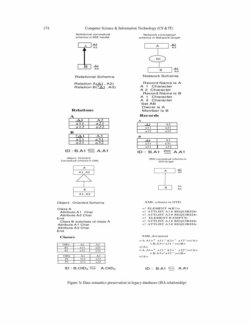
174 Computer Science & Information Technology (CS & IT)
A
B A1
A3
A1
A2
Relational conceptual
schema in EER model
Relational Schema
Relation A (A1 , A2)
Relation B (*A1 , A3)
ID : B.A1 A.A1
A3a31
*A1a11
Relations
A
B
A1a11
A2a21
a12 a22
a32a21
B
Set
AA1
A2
A1
A3
Network conceptual
schema in Network Graph
Network Schema
Record Name is A
A 1 Character
A 2 Character
Record Name is B
A 1 Character
A 3 Character
Set AB
Owner is A
Member is B
ID : B.A1 A.A1
A1
a11
Records
A
B
A1
a11
A2
a21
a12 a22
a21
A3
a31
a32
A
A1 , A2
B
A1 , A3
Object- Oriented
Conceptual schema in UML
Object- Oriented Schema
Class A
Attribute A1 Char
Attribute A2 Char
End
Class B subclass of class A
Attribute A1 Char
Attribute A3 Char
End
ID : B.OIDA A.OIDA
A2A1OIDA
a21#1
#2 a22a12
a11
Classes
A1OIDB
#1
#2 a12
a11
A3
a31
a32
B
AA1
A2
A1
A3
XML conceptual schema in
DTD Graph
XML schema in DTD
<! ELEMENT A(B?)>
<! ATTLIST A1 # REQUIRED>
<! ATTLIST A2 # REQUIRED>
<! ELEMENT B EMPTY>
<! ATTLIST A1 # REQUIRED>
<! ATTLIST A3 # REQUIRED>
ID : B.A1 A.A1
<A A1=”a11 " A2=”a12"></A>
< B A3="a31 " ></B>
</A>
<A A1=”a11 " A2=”a22"></A>
< B A3="a32 " ></B>
</A>
XML document
Figure 3c Data semantics preservation in legacy databases (ISA relationship)

Computer Science & Information Technology (CS & IT) 175
A
B
o
CA1
A4
A1
A3
A1
A2
Relational conceptual
schema in EER model
Relational Schema
Relation A (A1 , A2)
Relation B (*A1 , A3)
Relation C (*A1 , A4)
A3a31
*A1a11
Relations
A
B
A1a11
A2a21
a12 a22
a32a21
C
*A1 A4a11 a41a21 a42
B
Set AB
C
AA1
A2
A1
A3
Network conceptual
schema in Network Graph
Network Schema
Record Name is A
A 1 Character
A 2 Character
Record Name is B
A 1 Character
A 3 Character
Record Name is C
A 1 Character
A 4 Character
Set AB
Owner is A
Member is B
Set AC
Owner is A
Member is C
Set AC
RecordsA
B
A1
a11
A2
a21
a12 a22
C
A4
a41
a42
A1
a11
a12
*A1 A3a11 a31a21 a32
ID : B.A1 A.A1
ID : C.A1 A.A1
ID : B.A1 A.A1
ID : C.A1 A.A1
B1B A A1
idrefid
Flattened XML conceptual
schema in DTD Graph
ABC
idrefid
Flattened XML Document schema in DTD
<! ELEMENT ROOT (A , AB , B)>
<! ELEMENT A EMPTY >
<! ATTLIST A id ID # REQUIRED >
<! ATTLIST A A 1 CDATA # REQUIRED >
<! ELEMENT B EMPTY >
<! ATTLIST B id ID # REQUIRED >
<! ATTLIST B B 1 CDATA # REQUIRED >
<! ELEMENT AB EMPTY >
<! ATTLIST AB idref 1 IDREF # REQUIRED >
<! ATTLIST AB idref 2 IDREF # REQUIRED >
<! ATTLIST AB C CDATA # REQUIRED >
(b ) many-to- many cardinality
MVD : A.id �� B.id
MVD : B.id �� A.id
Flattened XML Document Data
< ROOT >
< A A1="a11 " id ="1"></A>
<B B1="b11 " id ="2"></B>
<A B C="c11 " idref1="1" idref2="2”></AB>
<A B C="c12 " idref1="2" idref2="1”></AB>
</ ROOT >
B A A1
idref id
Flattened XML conceptual
schema in DTD Graph
Flattened XML Document schema in DTD
<! ELEMENT ROOT (A , B)>
<! ELEMENT A EMPTY >
<! ATTLIST A id ID # REQUIRED >
<! ATTLIST A A 1 CDATA # REQUIRED >
<! ELEMENT B EMPTY >
<! ATTLIST B idref IDREF # REQUIRED >
<! ATTLIST B B 1 CDATA # REQUIRED >
FD : B.iderf � A.id
(a ) one-to- many cardinality
Flattened XML Document Data
B1
< ROOT >
< A A1="a11 " id ="1"></A>
< B B1="b11 " idref =1"></B>
< B B1="b12 " idref=1"></B>
</ ROOT >
Figure 4a Data semantics preservation in flattened XML documents (1:n & m:n cardinalities)

176 Computer Science & Information Technology (CS & IT)
< ROOT >
< A A1="a11 " id ="A1.1"></A>
< B A1="a11 " idref=A1.1"></B>
</ ROOT >
B A
idref id
Flattened XML conceptual
schema in DTD Graph
(c ) isa relationship
A1A1
Flattened XML Document schema in DTD
<! ELEMENT ROOT (A , B)>
<! ELEMENT A EMPTY >
<! ATTLIST A id ID # REQUIRED >
<! ATTLIST A A 1 CDATA # REQUIRED >
<! ELEMENT B EMPTY >
<! ATTLIST B idref IDREF # REQUIRED >
<! ATTLIST B A 1 CDATA # REQUIRED >
ID : B.idref � A.id
A1A C A1
idref
Flattened XML conceptual
schema in DTD Graph
B
idrefid
(d ) generalization
A1
Flattened XML Document Data
< ROOT >
< A A1="a11 " id ="1"></A>
< A A1="a12 " id ="2"></A>
<B A1="a 11 " idref=1"></B>
<C A1="a11 " idref =2"></C>
</ ROOT >
Flattened XML Document schema in DTD
<! ELEMENT ROOT (A,B,C)>
<! ELEMENT A EMPTY >
<! ATTLIST A id ID # REQUIRED >
<! ATTLIST A A1 CDATA # REQUIRED >
<! ELEMENT B EMPTY >
<! ATTLIST B idref IDREF # REQUIRED >
<! ATTLIST B A1 CDATA # REQUIRED >
<! ELEMENT C EMPTY >
<! ATTLIST C idref IDREF # REQUIRED >
<! ATTLIST C A1 CDATA # REQUIRED >
ID : B.idref � A.id
ID : C.idref � A.id
Figure 4b Data semantics preservation in flattened XML documents
(ISA, generalization)
2. RELATED WORK
On data transformation
Shoshani, A.[1] defined logical level approach data conversion by using source and target
schemas to perform data type conversion instead of physical data type conversion. He provided a
general methodology of using logical level approach of downloading source legacy database into
sequential file and uploading them into target legacy database for data transformation.
Lum et al [2] showed how to construct data conversion languages SDDL and TDL to extract and
restrict data from source legacy database into target legacy database.
The above two paper differ from this paper such that they apply sequential file as medium for
legacy databases exchange, but this paper applies flattened XML document as medium for legacy
databases exchange.
Fong and Bloor [3] described mapping navigational semantics of the network schema into a
relational schema before converting data from network database to relational database.

Computer Science & Information Technology (CS & IT) 177
Fong [4] presented a methodology of transforming object-oriented database objects into
Relational database by using SQL Insert statements.
Fong and Shiu [5] designed a Semantic Export Markup Language as a data conversion language
to export component of relational database into XML database.
Fong et al.[6] applied logical level approach for data materialization between relational database
and object-oriented database using sequential file as medium.
On Heterogeneous database
Given huge investment for a company put into heterogeneous databases, it is difficult for
company convert them into homogeneous databases for new applications. Therefore, researchers
have come up with a solution of universal databases that can be accessed as homogeneous
databases by the user [7] . For instance, we can provide an relational interface to non‐relational
database such as Hierarchical, Network, Object‐Oriented and XML [8] .
Hsiao & Kamel [9] offered a solution of multiple-models-and-languages-to-multiple-models-and–
languages mapping to access heterogeneous databases.
Their papers propose a universal database for Hierarchical, Network and Relational databases
while this paper proposes a universal database for Network, Relational, Object-Oriented and
XML databases.
On Universal database
Fong et al. [10] applied universal database system to access universal data warehousing for the
integration of both relational databases and object-oriented databases with star schema and OLAP
functions.
Silverston & Graziano [11] used a universal data model in a diagram to design the conceptual
schema of different legacy data models of any legacy database.
The above papers differ from this paper such that the above paper proposes a universal data
model diagram for universal database conceptual schema while this paper proposes using DTD
Graph in Figure 3 and 4 as conceptual schema for universal database.
On Homogeneous database
Sellis, Lin & Raschid [12] presented a solution to decompose and store the condition elements in
the antecedents of rules such as those used in production rule-based systems in homogeneous
databases environment using relational data model.
This paper differs from the above paper such that it uses flattened XML document environment
for universal database.
On schema translation
Funderburk et al. [13] proposed DTD Graph as XML conceptual schema which is identical to
DTD, but in a graph format.
On Cloud Database
Derrick Harris [14] defines cloud database as databases in virtual machines.
This paper plans to include cloud computing for further research in future.
On Flattened XML document
Fong et al. [15] converted an XML document into Relational database by transforming XML
document into flattened XML document with relational table structure by Extensible Stylesheet
Language Transformation.
Compared with the above references, this paper has 3 uniqueness:
(1) Cover more data model
All other database research paper only involve 2 or 3 data models in the universal database. This
paper involves 4 data models such as Network, relational, object-oriented and XML.
(2) Use cloud platform

178 Computer Science & Information Technology (CS & IT)
The reference papers do not use cloud platform to implement universal database. This paper
performs prototype in cloud platform.
(3) Flattened XML document as middleware
This paper applies flattened XML document as medium to transform legacy databases among
each other which is not done by other research papers.
Above all, this paper extends the work of universal database into an “open” universal database
gateway such that the universal database is not limited to a particular DBMS, but can be any
legacy database of user’s choice. Similarly, OUDG is more user friendly than ODBC because it
requires less programming effort.
3. METHODOLOGY OF OUDG AS ODBC SUPPLEMENT
This paper proposes OUDG as a database middleware to access legacy databases via flattened
XML documents as an universal database as follows:
First Legacy databases � Phase 1: Second Flattened XML documents (universal database)
� Phase 2:Third Legacy databases
The major functions of OUDG are:
Phase I: Transform first legacy databases into flattened XML documents
Any one of the four first legacy database can be transformed into the flattened XML document as
follows:
Case 1: Transform first legacy relational databases into second flattened XML documents
Firstly, we perform the preprocess of mapping relational schema into flattened XML schema.
Secondly, we perform their correspondent data conversion. The input is a relational database and
the output is an flattened XML document. The system will read relational table according to the
legacy relational schema. In one-to-many data semantic, it will post parent and child relations into
2 table structured sibling XML elements linked with id and idref. In many-to-many data semantic,
it will post 2 relations and their relationship relation into 3 table structured XML sibling elements
linked with idref(s) and id(s). In isa data semantic, it will post superclass and subclass relations
into 2 table structured XML sibling elements linked with id and idref with the same key as shown
in Figure 3 and Figure 4.
Case 2: Transform first XML databases into second flattened XML documents
Firstly, we perform the preprocess of mapping XML schema into flattened XML schema.
Secondly, we perform their correspondent data conversion. The input is an XML database and the
output is a flattened XML document with relational table structure. The system will read XML
document according to the XML schema. In one-to-many data semantic, it will post element and
sub-element into 2 XML sibling elements linked with id and idref. In many-to-many data
semantic, it will post 3 elements linked with id(s) and idref(s) into 3 XML sibling elements linked
with id(s) and idref(s). In isa data semantic, it will post superclass and subclass elements into 2
XML sibling elements linked with id and idref with the same key as shown in Figure 3 and Figure
4.
Case 3: Transform first legacy Object Oriented database into second flattened XML document
Firstly, we perform the preprocess of mapping object-oriented schema into flattened XML
schema. Secondly, we perform their correspondent data conversion. The input is an OODB and
the output is a flattened XML document. The system will read OODB according to OODB
schema. In one-to-many data semantic, it will post object and set of associated objects into 2
XML sibling elements linked with id and idref. In man-to-many data semantic, it will post 2 sets
of associated objects with a common object into 3 XML sibling elements such that a sibling

Computer Science & Information Technology (CS & IT) 179
element with 2 IDREF(s) referring 2 sibling elements with 2 ID(s)). In isa data semantic, it will
post superclass and subclass objects with same OID into 2 XML sibling elements linked with id
and idref with the same key as shown in Figure 3 and Figure 4.
Case 4: Transform first legacy Network databases into second flattened XML documents
Firstly, we perform the preprocess of mapping network schema into flattened XML schema.
Secondly, we perform their correspondent data conversion. The input is a Network
database(NDB) and the output is a table structured flattened XML document. The system will
read NDB according to NDB schema. In one-to-many data semantic, it will post owner and
member records into 2 XML sibling elements linked with id and idref. In many-to-many data
semantic, it will post 2 owners and 1 common member records into 3 XML sibling elements
linked with id(s) and idref(s). In isa data semantic, it will post an owner and a member records
into 2 XML sibling elements linked with id and idref with the same key as shown in Figure 3 and
Figure 4.
Phase II: Transform second flattened XML documents into third legacy databases
In step 2, we map the flattened XML schema into another legacy database schema, followed by
the data transformation of the flattened XML documents into a legacy database according to the
mapped legacy database schema. In this way, each source database data type can be read by the
legacy database schema. Therefore, there is no need for physical data type conversion in this
approach. Therefore, we can post the flattened XML document into a legacy database of
relational, object-oriented, network or XML.
Case 5: Transform second flattened XML documents into third relational databases
Firstly, we perform the preprocess of mapping flattened XML schema into relational schema.
Secondly, we perform their correspondent data conversion. The input is a flattened XML
document and the output is a relational database. The system will read flattened XML document
according to flattened XML document schema. In one-to-many data semantic, it will post 2 XML
sibling elements into parent and child relations. In many-to-many data semantic, it will post 3
XML sibling elements linked with id(s) and idref(s) into 2 parents and 1 child relations. In isa
data semantic, it will post 2 XML sibling elements into superclass relation and sub-class relation
as shown in Figure 3 and Figure 4.
Case 6: Transform second flattened XML documents into third object-oriented databases
Firstly, we perform the preprocess of mapping flattened XML schema into object-oriented
schema. Secondly, we perform their correspondent data conversion. The input is a flattened XML
document and the output is an object-oriented database. The system will read flattened XML
document according to flattened XML document schema. In one-to-many data semantic, it will
post 2 XML sibling elements into 2 associated objects with OID and Stored OID. In many-to-
many data semantic, it will post 3 XML sibling elements linked with id(s) and idref(s) into 3
associated objects. In isa data semantic, it will post 2 XML sibling elements into 2 superclass and
sub-class objects as shown in Figure 3 and Figure 4.
Case 7 Transform second flattened XML documents into third network databases:
Firstly, we perform the preprocess of mapping flattened XML schema into network schema.
Secondly, we perform their correspondent data conversion.
The input is a flattened XML document and the output is a network database. The system will
read flattened XML document according to flattened XML document schema. In one-to-many
data semantic, it will post 2 XML sibling elements into 2 owner and member records. In many-to-
many data semantic, it will post 3 XML sibling elements linked with id(s) and idref(s) into 2
owners linked with 1 member record with the same key. In isa data semantic, it will post 2 XML

180 Computer Science & Information Technology (CS & IT)
sibling elements into 2 owner and member record with the same key as shown in Figure 3 and
Figure 4.
Case 8: Transform second flattened XML documents into third legacy XML databases
Firstly, we perform the preprocess of mapping flattened XML schema into XML schema.
Secondly, we perform their correspondent data conversion.
The input is a flattened XML document and the output is an XML document. The system will
read flattened XML documents according to flattened XML documents schema. In one-to-many
data semantic, it will post 2 XML sibling elements into 2 XML element and sub-elements. In
many-to-many data semantic, it will post 3 XML sibling elements linked with id(s) and idref(s)
into 2 pairs of XML elements linked with same sub-element. In isa data semantic, it will post 2
XML sibling elements with the same key into XML element and sub-elements with the same key
as shown in Figure 3 and Figure 4.
4. CASE STUDY
A logistic system records the customer shipment information including which orders are being
packed and what the packing information is. Based on the XML schema below, there are three
intermediate independent entities: PL_INFORMAION recording the general information of the
shipment, PL_LINE_INFORMATION storing the packing information ― particularly
information about the BOXES ― and ORDER_INFORMATION storing the information of
orders such as the product information. A many-to-many relationship between
ORDER_INFORMATION and PL_LINE_DETAIL must be resolved early in the modeling
process to eliminate repeating information when representing PL_INFORMATION or
ORDER_INFORMATION (MySQL 2013). The strategy for resolving many-to-many
relationship[s] is to replace the relationship with two one-to-many cardinality with an association
entity and then relate the two original entities to the association entity. As a result, these two one-
to-many relationships are between PL_LINE_INFORMATION and PL_LINE_DETAIL, and
between ORDER_INFORMATION and PL_LINE_DETAIL. Similarly, the ORDER_INFOR
MATION can be divided into BulkOrder and CustomerOrder in generalization as shown in
Figure 6.
In Figure 6, there are six relations in relational database. Each table has its primary key and
foreign key. Their data dependencies are such that each foreign key determines its referred
primary key in functional dependency (FD) in one-to-many cardinality with foreign key on the
“many” side, and subclass foreign key is a subset of its referred primary key in inclusion
dependency (ID). For relations in many-to-many cardinality, their primary keys are in multi-
valued dependencies(MVD) to each other as follows:
FD: PL_Line_Information.PL_Information_Seqno � PL_Information.PL_Information_Seqno
ID: Bulk_Order.BulkOrder.Order_Number Order_Information.Order_Number
ID: TailorMadeOrder.Order_Number Order_Information.Order_Number
MVD: PL_Line_Information.PL_Information_Seqno �� Order_Information.Order_Number
MVD: Order_Information.Order_Number �� PL_Line_Information.PL_Information_Seqno
In Figure 7, the relations are transformed into flattened XML document. The input relational
conceptual schema is Extended Entity Relationship model(Chen, 1976). We map input relational
schema into an flattened XML OUDG schema with relational structure in two levels tree. Notice
that the second level elements (under root elements) are linked together using idref referring to id,
which is similar to foreign key referring to primary key. There are seven elements. The second
level elements has id(s) and/or idref(s). Their data dependencies are such that each idref

Computer Science & Information Technology (CS & IT) 181
determines its referred id in FD for one-to-many cardinality, and each subclass idref is a subset of
its superclass id in ID. For elements in many-to-many cardinality, their id(s) are in MVD as
follows:
FD: idref1 � id1
ID: idref3 id3
MVD: id2 �� id3
MVD: id3 �� id2
In Figure 8, the flattened XML document is transformed into XML document. Elements
Pl_information and Pl_line_information are in element and sub-element 1:n association. Elements
Pl_line_information and Order_information are in m:n association through element
Pl_line_detail linked by pairs of idref referring to id. Elements Order_information and
Bulk_Order are in isa association. Elements Order_information and TailorMadeOrder are also in
isa association. Their data dependencies are such that each sub-element can determine its element
in FD. Each sub-class key is a subset of its superclass key in ID. Two one-to-many cardinality
with the same element on the “many” side is equivalent to a many-to-many cardinality of the two
“one” side elements in MVD as follows:
FD: PL_Line_Information.PL_Information_Seqno � PL_Information.PL_Information_Seqno
ID: BulkOrder.TechnicalOrderNo Order_Information.Order_Seqno
ID: TailorMadeOrder.CustomerOrderNo Order_Information.Order_Seqno
MVD: PL_Line_Information.PL_Information_Seqno �� Order_Information.Order_Seqno
MVD: Order_Information.Order_Seqno �� PL_Line_Information.PL_Information_Seqno
In Figure 9, the flattened XML document is transformed into Object-Oriented database. It shows
the mapping of flattened XML schema into UML as object-oriented conceptual schema. There
are six classes. Each class has its OID (object identity), which is similar to primary key in
relational schema, and Stored OID, which is similar to foreign key in relational schema. Their
data dependencies are such that each Stored OID key determines its referred OID in FD, and each
subclass OID is a subset of its superclass OID in ID. The class PL_Informationa nd class
PL_Line_Information are in 1:n association in FD. Classes PL_line_Informaton and class
Order_Information are in m:n association through class PL_Line_Detail. Subclass BulkOrder and
subclass TailorMadeOrder are in generalization under same superclass Order_Information in ID
as follows:
FD: PL_Line_Information.Stored_OID � PL_Information.OID
ID: Bulk_Order.OID Order_Information.OID
ID: TailorMadeOrder.OID Order_Information.OID
MVD: PL_Line_Information.OID �� Order_Information.OID
MVD: Order_Information.OID �� PL_Line_Information.OID
In Figure 10, flattened XML document is transformed into Network database. Record
Pl_informations and record Order_information are under network DBMS as first records for
database navigation access path. The path can go from record Pl_information to
Pl_line_information in owner and member record in 1:n relationship in FD. Records
Pl_line_information (owner), Order_information(owner) and Pl_line_detail (member) are in flex
structure such that records Pl_line_information and Order_information they are in m:n
relationship in MVD. Records Order_information and BulkOrder are in isa relationship since they
have same key value in ID. Similarly, records Order_information and TailorMadeOrder are in isa
relationship due to same key value in ID. The set records are pointers only. Their data
dependencies are as follows:
FD: PL_Line_Information.PL_Information_Seqno � PL_Information.PL_Information_Seqno
ID: Bulk_Order.TechnicalOrderNo Order_Information.OrderSeqno
ID: TailorMadeOrder.CustomerOrderNo Order_Information.OrderSeqno
MVD: PL_Line_Information.PL_Information_Seqno �� Order_Information.OrderSeqno

182 Computer Science & Information Technology (CS & IT)
MVD: Order_Information.OrderSeqno �� PL_Line_Information.PL_Information_Seqno
Papers in this format must not exceed twenty (20) pages in length. Papers should be submitted to
the secretary AIRCC. Papers for initial consideration may be submitted in either .doc or .pdf
format. Final, camera-ready versions should take into account referees’ suggested amendments.
PL_INFORMATION
PL_LINE_INFORMATION
PL_LINE_DETAIL
ORDER_INFORMATION
BulkOrder TailorMadeOrder
Pl_information_seqno
Pl_line_information_seqno
Order_number
1..1
1:m1:m 1:m
Order_number Order_number
Mapped Object-Oriented conceptual schema

Computer Science & Information Technology (CS & IT) 183
5. CONCLUSION
Since relational database is the most user friendly legacy database, and XML database is the most
portable database for information highway on the Internet. In this project, we propose a Flattened
XML database as universal database such that it is most user friendly and portable as a database
middleware for all legacy databases.
The uniqueness of this paper are:
(1) Openness of an universal database: The reason we choose flattened XML document is due to
its openness, and DBMS independence. All other data models are DBMS dependent.
Nevertheless, users can use OUDG to access any legacy database via flattened XML documents
on the Internet by Internet Explorer without programming.
(2) Recovery of legacy database: Since flattened XML document is a replicate legacy database, it
can be used to recover any legacy database whenever the production legacy database is down. As
a result, replicate XML document can be parallel processing with legacy database in non-stop
computing.
(3) Heterogeneous database integration for data warehousing: By transforming all in-house legacy
databases into one legacy database as the data cube, companies can use OUDG to integrated their
legacy databases into a data warehousing for decision support system.
(4) Portability of Flattened XML document as Universal database: The OUDG solution is not
limited to using a particular DBMS, but allows users of any legacy database access other legacy
database.
In summary, the proposed OUDG unites all legacy databases data models into flattened XML
schema. The portability of the proposed flattened XML document can be transferred into any
open platform. The data conversion methodology of this OUDG is to download the raw data of
source database into flattened XML document using source database schema, and upload the
flattened XML document into target database using translated target database schema, which is a
logical level approach, and which can avoid physical data type conversion. Therefore, the
methodology can transform any legacy database into any other legacy database. The reason of
using flattened XML document as medium is to reduce the number of programs for the data
conversion; otherwise, we need 4 * 4 = 16 programs, instead of the current 4 + 4 = 8 programs to
do the data conversion for the four legacy database models: relational, network, object-oriented
and XML. Above all, all legacy databases can be transformed into each other via flattened XML
documents for data access in the same way as computers connect to each other via computer
network for information retrieval.
REFERENCES
[1] Shoshani, A., (1975) “A Logical-Level Approach to Data Base Conversion”, ACM SGMOD
International Conference on Management of Data, pp.112-122.
[2] Lum, V.Y., Shu N.C. & Housel B.C. (1976) “A General Methodology for Data Conversion and
Restructuring”, IBM Journal of research and development, Volume 20, Issue 5, pp.483-497.
[3] Fong, J.& Bloor C. (1994) “Data Conversion Rules from Network to Relational Databases”,
Information and Software Technology, Volume. 36 No. 3, pp. 141-154.
[4] Fong, J. (1997) “Converting Relational to Object-Oriented Databases”, SIGMOD RECORD, Volume
26, Number 1, pp53-58.
[5] Fong, J. & Shiu, H. (2012) “An interpreter approach for exporting relational data into XML
documents with Structured Export Markup Language”, Journal of Database Management, volume 23,
issue 1.
[6] Fong, J., Pang, R., Fong, A., Pang, F. & Poon, K. (2003) “Concurrent data materialization for object-
relational database with semantic metadata”, International Journal of Software Engineering and
Knowledge Engineering, Volume 13, Number 3, pp.257-291.
[7] Fong, J. & Huang, S. (1999) “Architecture of a Universal Database: A Frame Model Approach”,
International Journal of Cooperative Information Systems, Volume 8, Number. 1, pp. 47-82.
[8] Fong, J. (1996) “Adding Relational Interface to Non-relational Database",IEEE Software, pp. 89-97.
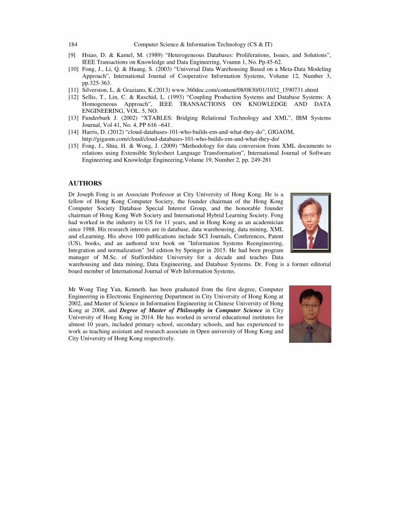
184 Computer Science & Information Technology (CS & IT)
[9] Hsiao, D. & Kamel, M. (1989) “Heterogeneous Databases: Proliferations, Issues, and Solutions”,
IEEE Transactions on Knowledge and Data Engineering, Voumn 1, No. Pp.45-62.
[10] Fong, J., Li, Q. & Huang, S. (2003) “Universal Data Warehousing Based on a Meta-Data Modeling
Approach”, International Journal of Cooperative Information Systems, Volume 12, Number 3,
pp.325-363.
[11] Silverston, L. & Graziano, K.(2013) www.360doc.com/content/08/0830/01/1032_1590731.shtml
[12] Sellis, T., Lin, C. & Raschid, L. (1993) “Coupling Production Systems and Database Systems: A
Homogeneous Approach”, IEEE TRANSACTIONS ON KNOWLEDGE AND DATA
ENGINEERING, VOL. 5, NO.
[13] Funderburk J. (2002) “XTABLES: Bridging Relational Technology and XML”, IBM Systems
Journal, Vol 41, No. 4, PP 616 –641.
[14] Harris, D. (2012) “cloud-databases-101-who-builds-em-and-what-they-do”, GIGAOM,
http://gigaom.com/cloud/cloud-databases-101-who-builds-em-and-what-they-do/
[15] Fong, J., Shiu, H. & Wong, J. (2009) “Methodology for data conversion from XML documents to
relations using Extensible Stylesheet Language Transformation”, International Journal of Software
Engineering and Knowledge Engineering,Volume 19, Number 2, pp. 249-281
AUTHORS
Dr Joseph Fong is an Associate Professor at City University of Hong Kong. He is a
fellow of Hong Kong Computer Society, the founder chairman of the Hong Kong
Computer Society Database Special Interest Group, and the honorable founder
chairman of Hong Kong Web Society and International Hybrid Learning Society. Fong
had worked in the industry in US for 11 years, and in Hong Kong as an academician
since 1988. His research interests are in database, data warehousing, data mining, XML
and eLearning. His above 100 publications include SCI Journals, Conferences, Patent
(US), books, and an authored text book on "Information Systems Reengineering,
Integration and normalization" 3rd edition by Springer in 2015. He had been program
manager of M.Sc. of Staffordshire University for a decade and teaches Data
warehousing and data mining, Data Engineering, and Database Systems. Dr. Fong is a former editorial
board member of International Journal of Web Information Systems.
Mr Wong Ting Yan, Kenneth. has been graduated from the first degree, Computer
Engineering in Electronic Engineering Department in City University of Hong Kong at
2002, and Master of Science in Information Engineering in Chinese University of Hong
Kong at 2008, and Degree of Master of Philosophy in Computer Science in City
University of Hong Kong in 2014. He has worked in several educational institutes for
almost 10 years, included primary school, secondary schools, and has experienced to
work as teaching assistant and research associate in Open university of Hong Kong and
City University of Hong Kong respectively.

David C. Wyld et al. (Eds) : ITCS, CST, JSE, SIP, ARIA, DMS - 2015
pp. 185–197, 2015. © CS & IT-CSCP 2015 DOI : 10.5121/csit.2015.50118
CLUSTERED COMPRESSIVE SENSING-
BASED IMAGE DENOISING USING
BAYESIAN FRAMEWORK
Solomon A. Tesfamicael * †
Faraz Barzideh ‡
*
Sør-Trondlag University College (HiST), Trondheim, Norway †Norwegian University of Science and Technology (NTNU),
Trondheim, Norway [email protected]/[email protected]
‡ Department of Electrical Engineering and Computer Science,
University of Stavanger (UiS), Stavanger, Norway [email protected]
ABSTRACT
This paper provides a compressive sensing (CS) method of denoising images using Bayesian
framework. Some images, for example like magnetic resonance images (MRI) are usually very
weak due to the presence of noise and due to the weak nature of the signal itself. So denoising
boosts the true signal strength. Under Bayesian framework, we have used two different priors:
sparsity and clusterdness in an image data as prior information to remove noise. Therefore, it is
named as clustered compressive sensing based denoising (CCSD). After developing the
Bayesian framework, we applied our method on synthetic data, Shepp-logan phantom and
sequences of fMRI images. The results show that applying the CCSD give better results than
using only the conventional compressive sensing (CS) methods in terms of Peak Signal to Noise
Ratio (PSNR) and Mean Square Error (MSE). In addition, we showed that this algorithm could
have some advantages over the state-of-the-art methods like Block-Matching and 3D
Filtering (BM3D).
KEYWORDS
Denoising, Bayesian framework, Sparse prior, Clustered prior, posterior, Compressive sensing,
LASSO, Clustered Compressive Sensing
1. INTRODUCTION
Image denoising is an integral part of image processing. There are different sources of noise for
images and different noise models are assumed to remove or reduce noise (to denoise),
accordingly. Mostly image noises are modelled by additive white Gaussian distribution while
others like ultrasound and MRI images can be modelled by speckle and Rican distribution
respectively [1]. In the past decades, removing the noises has been given ample attention and
there are several ways to de-noise an image. A good image denoising technique removes the
noise to a desirable level while keeping the edges. Traditionally, this has been done using spatial
filtering and transform domain filtering. The former uses median filter, Weiner filter and so on
while the later uses Fast Fourier Transform (FFT) and Wavelet Transform (WT) to transform the

186 Computer Science & Information Technology (CS & IT)
image data to frequency or time-frequency domain, respectively. The later transform method have
been used intensively due to the fact that the Wavelet transform based methods surpasses the
others in the sense of mean square error (MSE) or pick signal to noise ratio (PSNR) and other
performance metrics [1], [2], [3].
Recently, another way of image denoising has been used after a new way of signal processing
method called compressive sensing (CS) was revived by authors like Donoho, Candés, Romberg
and Tao [4]- [7]. CS is a method to capture information at lower rate than the Nyquist- Shannon
sampling rate when signals are sparse or sparse in some domain. It has already been applied in
medical imaging. In [8] the authors have used the sparsity of magnetic resonance imaging (MRI)
signals and showed that this can be exploited to significantly reduce scan time, or alternatively,
improve the resolution of MR imagery and in [9] it is applied for Biological Microscopy image
denoising to reduce exposure time along with photo- toxicity and photo-bleaching. Since CS-
based denoising is done using reduced amount of data or measurement. Actually, it can remove
noise better than the state-of the art methods while using few measurements and preserving the
perceptual quality [10]. This paper builds up on the CS based denoising and incorporates it with
the clustredness of some image data. This is done using a statistical method called Bayesian
framework.
There are two schools of thoughts called the classical (also called the frequentist) and the
Bayesian in the statistical world. Their basic difference arises from the basic definition of
probability. Frequentists define P(x) as a long-run relative frequency with which x occurs in
identical repeats of an experiment. Where as Bayesian defines P(x|y) as a real number measure of
the probability of a proposition x, given the truth of the information represented by proposition y.
So under Bayesian theory, probability is considered as an extension of logic. Probabilities
represent the investigators degree of belief- hence it is subjective. That belief or prior information
is an integral part of the inference done by the Bayesian [11] - [20]. For its flexibility and
robustness this paper focuses on Bayesian approach. Specifically the prior information’s like
sparsity and clusterdness (or structures on the patterns of sparsity) of an image as two different
priors are used and the noise is removed by using reconstructing algorithms.
Our contribution in this work is to use the Bayesian framework and incorporate two different
priors in order to remove the noise in an image data and in addition we compare different
algorithms. Therefore, this paper is organized as follows. In section II we discuss the problem of
denosing using the CS theory under the Bayesian framework, that is using two priors on the data,
the sparse and clustered priors, and define the denosing problem in this context. In section III we
provide how we implemented the analysis. Section IV shows our results using synthetic and MRI
data, and section V presents conclusion and future work.
2. COMPRESSED SENSING BASED DENOISING
In Wavelet based transform denosing the image data is transformed to time-frequency domain
using Wavelet. Only the largest coefficients are kept and the rest are thrown away using
thresholding. Then by applying the inverse Wavelet transform the image is denoised [21],
however, in this paper we used CS recovery as denosing.
Considering an image which is sparse or sparse in some domain, which has sparse representation
in some domain or most of the energy of the image is compressed in few coefficients, say � ϵ ℝ�
with non zero elements k, corrupted by noise n ϵ ℝ�. It is possible to use different models of
noise distribution. By using a measurement matrix A ϵ ℝ�×�, we get a noisy and under sampled
measurements ϵ ℝ�. Further we assume that w = An ϵ ℝ� is i.i.d. Gaussian random variables
with zero mean and covariance matrix σ�I, due to the central limit theorem. This assumption can
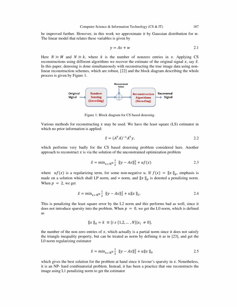
Computer Science & Information Technology (CS & IT) 187
be improved further. However, in this work we approximate it by Gaussian distribution for �.
The linear model that relates these variables is given by
= �� � � 2.1
Here � ≫ � and � ≫ �, where � is the number of nonzero entries in �. Applying CS
reconstructions using different algorithms we recover the estimate of the original signal �, say ��.
In this paper, denosing is done simultaneously with reconstructing the true image data using non-
linear reconstruction schemes, which are robust, [22] and the block diagram describing the whole
process is given by Figure 1.
Figure 1: Block diagram for CS based denosing.
Various methods for reconstructing � may be used. We have the least square (LS) estimator in
which no prior information is applied:
�� = ���������, 2.2
which performs very badly for the CS based denoising problem considered here. Another
approach to reconstruct � is via the solution of the unconstrained optimization problem
�� = min� ℝ!��
‖ # ��‖�� � $%��� 2.3
where $%��� is a regularizing term, for some non-negative $. If %��� = ‖� ‖&, emphasis is
made on a solution which shall LP norm, and = norm, and ‖� ‖& is denoted a penalizing norm.
When ' = 2, we get
�� = min� ℝ!��
‖ # ��‖�� � $‖� ‖�. 2.4
This is penalizing the least square error by the L2 norm and this performs bad as well, since it
does not introduce sparsity into the problem. When ' = 0, we get the L0 norm, which is defined
as
‖� ‖+ = � ≡ -. / -1,2, … , �3|�5 6 03,
the number of the non zero entries of �, which actually is a partial norm since it does not satisfy
the triangle inequality property, but can be treated as norm by defining it as in [23], and get the
L0 norm regularizing estimator
�� = min� ℝ!��
‖ # ��‖�� � $‖� ‖+ 2.5
which gives the best solution for the problem at hand since it favour’s sparsity in �. Nonetheless,
it is an NP- hard combinatorial problem. Instead, it has been a practice that one reconstructs the
image using L1 penalizing norm to get the estimator

188 Computer Science & Information Technology (CS & IT)
�� = min� ℝ!��
‖ # ��‖�� � $‖� ‖� 2.6
which is a convex approximation to the L0 penalizing solution II.5. These estimators, 2.4 - 2.6,
can equivalently be presented as solutions to constrained optimization problem [4] - [7], and in
the CS literature there are many different types of algorithms to implement them. A very popular
one is the L1 penalized L2 minimization called LASSO (Least Absolute Shrinkage and Selection
Operator), which we later will present it in Bayesian framework. So first we present what a
Bayesian approach is and come back to the problem at hand.
2.1. Bayesian framework
Under Bayesian inference consider two random variables � and with probability density
function (pdf) '��� and '��, respectively. Using Bayes’ theorem it is possible to show that the
posterior distribution, '��|�, is proportional to the product of the likelihood function, '�|��, and the prior distribution, '���,
'��|� ∝ '�|��'��� 2.7
Equation (2.7) is called Updating Rule in which the data allows us to update our prior views
about �. And as a result we get the posterior which combines both the data and non-data
information of � [11], [12], [20].
Further, the Maximum a posterior (MAP), ��89, is given by
��89 = arg max> '�|��'���
To proceed further, we assume two prior distributions on �.
2.2. Sparse Prior
The reconstruction of � resulting from the estimator (2.3) for the sparse problem we consider in
this paper given by, (2.4) - (2.5), can be presented as a maximum a posteriori (MAP) estimator
under the Bayesian framework as in [23]. We show this by defining a prior probability
distribution for � on the form
'��� = ?@AB�C�
D ?@AB�C�E>C F ℝG 2.8
where the regulirizing function % ∶ I → K is some scalarvalued, non negative function with
I ⊆ ℝ which can be expanded to a vector argument by
%��� = ∑ %��5�N5O� 2.9
such that for sufficiently large $, D P�QR�>�S�> T ℝG is finite. Further, let the assumed variance of
the noise be given by
U� = V$
where V is system parameter which can be taken as V = U�$. Note that the prior, (2.8), is
defined in such a way that it can incorporate the different estimators considered above by

Computer Science & Information Technology (CS & IT) 189
assuming different penalizing terms via %��� [23]. Further, the liklihood function, '�|��, can be
shown to be
pX|��y|x� = ���Z[�!/] e� _
]`]‖X�a�‖]] 2.10
the posterior, p�x|y�,
p�|X�x|y; A� =e� �
�[]‖X�a�‖]]
�2πσ��/� D d@e� _]f‖g@hi‖]
]jfk�i��l�i m ℝ!
and the MAP estimator becomes
x��n = arg min� ℝ!��
‖y # Ax‖�� � λf�x� 2.11
as shown in [20]. Note that (2.11) which is equivalent to (2.3). Now, as we choose different
regularizing function, which enforces sparsity into the vector x, we get different estimators listed
below [23]:
1) Linear Estimators: when f�x� = ‖x‖�� (2.11) reduces to
x�qrsdtu = AvwAAv � λIx��
y, 2.12
which is the LMMSE estimator. But we ignore this estimator in our analysis since the
following two estimators are more interesting for CS problems.
2) LASSO Estimator: when f�x� = ‖x‖� we get the LASSO estimator and (II.11) becomes,
x�qayyz = arg min� ℝ!��
‖y # Ax‖�� � λ‖x‖�, 2.13
which is the same as (2.6).
3) Zero-Norm regularization estimator: when %�x� = ‖x‖+, we get the Zero-Norm
regularization estimator (2.5) to reconstruct the image from the noisy data and (2.11)
becomes
x�{du|��|u} = arg min� ℝ!��
‖y # Ax‖�� � λ‖x‖+, 2.14
which is identical to 2.5. As mentioned earlier, this is the best solution for reconstruction of the
sparse vector �, but is NP-complete. The worst reconstruction for the sparse problem considered
is the L2- regularization solution given by (2.12). However, the best one is given by the equation
(2.13) and its equivalent forms such as L1-norm regularized least-squares (L1-LS) and others [5]-
[7].
2.3. Clustering Prior
Building on the Bayesian philosophy, we can further assume another prior distributions for
clustering. The entries of the sparse vector � may have some structure that can be represented
using distributions. In [18] a hierarchical Bayesian generative model for sparse signals is found in

190 Computer Science & Information Technology (CS & IT)
which they have applied full Bayesian analysis by assuming prior distributions to each parameter
appearing in the analysis. We follow a different approach. Instead we use another penalizing
parameter to represent clusterdness in the data. For that we define the clustering using the
distance between the entries of the sparse vector � by
~��� ≡ ∑ |�5 # �5��|N5O� ,
and we use a regularizing parameter . Hence, we define the clustering prior to be
���� = ?@���C�
D ?@���C�E>i m ℝ! 2.15
The new posterior involving this prior under the Bayesian framework is proportional to the
product of the three pdf’s:
p�x|y) ∝ p(y|x)p(x)q(x). 2.16
By similar arguments as used in 2.2 we arrive at the Clustered LASSO estimator
x�����qayyz = arg min� ℝ!�
�‖y − Ax‖�
� + λ‖x‖� + � ∑ |�5 − �5��|N5O� , 2.17
where λ, γ are our tuning parameters for the sparsity in � and the way the entries are clustered,
respectively.
3. IMPLEMENTATION OF THE ANALYSIS
The main focus of this paper is to give a practical application of compressed sensing, namely
denoising. That is we interpret the reconstruction of images by CS algorithms, given relatively
few measurements y and measurement matrix A, as denosing. That means the CS based denosing
happens when we apply the reconstructing schemes. Actually, we have used both CS based
(LMMSE, LASSO and Clustered LASSO given by equations (2.12), (2.13), (2.17) respectively)
and non-CS based denoising procedures (LS (2.2); BM3D). So that we compare the merits and
draw backs of CS based denoising techniques.
In the equations (2.12) , (2.13), and (2.17) we have parameters like λ and γ. As we have based our
analysis in Bayesian framework we could have assumed some prior distributions on each of them,
and build a hierarchical Bayesian compressive sensing. Instead we have used them as a tuning
parameter for the constraint and we have tried to use them in the optimal way. Still it needs more
work! However, we have found an optimal λ value for the LMMSE in (2.12), that is λ = 1e−07. In
implementing (2.13), that is least square optimization with L1 regularization, we have used the
Quadratic programming with constraints similar to Tibshirani [24], [25]. That is solving
x� = arg min� ‖y − Ax‖�� 3.1
�$��P�� �� ‖x‖� ≤ t,
instead of (2.13). We see that � and λ are related.
In addition, equation (II.17) is implemented similar to LASSO with additional term on the
constraint. That is we bounded ~(�) ≤ S. This S is some how related to γ, i.e., we put constrain
on the neighboring elements. Since we have vectorized the image for the sake of efficiency of the
algorithm, the penalizing terms are applied column wise. Other ways of implementing

Computer Science & Information Technology (CS & IT) 191
(constraining) are also possible. But we differ it for future work. In our simulations we have used
optimal values of these constraints. Figure 2 and 3 show the respective optimal values for one of
the simulations in the next section.
Figure 1: This figure shows the MSE of LASSO and clustered LASSO for different values of � for figure
4. It can be seen that there is only one optimal value.
Figure 2: This figure shows the MSE of LASSO and clustered LASSO for different values of � for figure
4. It can be seen that there is only one optimal value d and by loosening the constraint clustered LASSO
will converge to LASSO.
4. RESULTS
4.1 First set of Synthetic Data
In order to demonstrate the performance of reconstruction of the sparse signal (denosing)
presented in the paper we have used synthetic data. The first set of data is the image with several
English letters, where the image itself is sparse and clustered in the spatial domain. We have
applied Gaussian noise with mean zero and variance σ2 = 0.2 and random matrix � with Gaussian
entries with variance σ2 = 1. For LMMSE we used λ = 1e − 07 in our simulations. However, we
have used equivalent constraints for λ and γ for the LASSO and clustered LASSO.
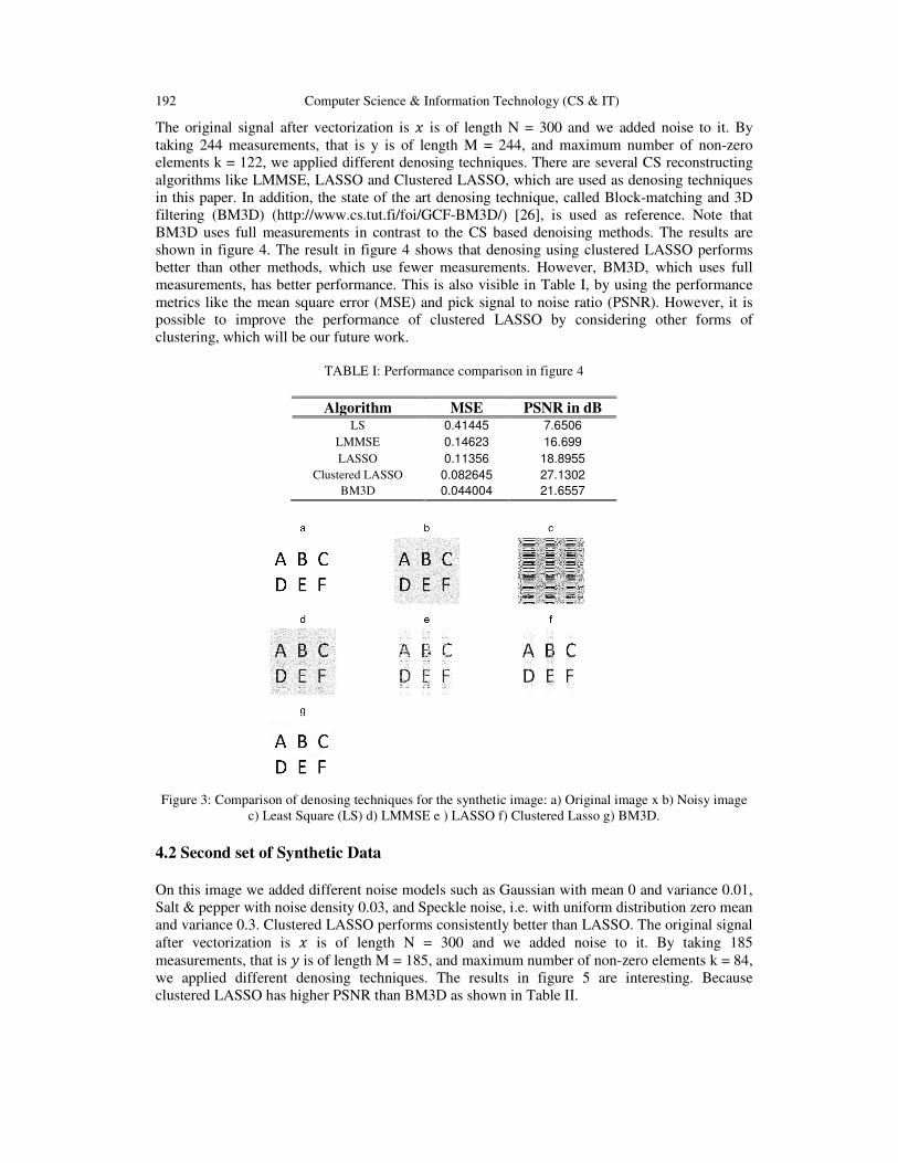
192 Computer Science & Information Technology (CS & IT)
The original signal after vectorization is � is of length N = 300 and we added noise to it. By
taking 244 measurements, that is y is of length M = 244, and maximum number of non-zero
elements k = 122, we applied different denosing techniques. There are several CS reconstructing
algorithms like LMMSE, LASSO and Clustered LASSO, which are used as denosing techniques
in this paper. In addition, the state of the art denosing technique, called Block-matching and 3D
filtering (BM3D) (http://www.cs.tut.fi/foi/GCF-BM3D/) [26], is used as reference. Note that
BM3D uses full measurements in contrast to the CS based denoising methods. The results are
shown in figure 4. The result in figure 4 shows that denosing using clustered LASSO performs
better than other methods, which use fewer measurements. However, BM3D, which uses full
measurements, has better performance. This is also visible in Table I, by using the performance
metrics like the mean square error (MSE) and pick signal to noise ratio (PSNR). However, it is
possible to improve the performance of clustered LASSO by considering other forms of
clustering, which will be our future work.
TABLE I: Performance comparison in figure 4
Algorithm MSE PSNR in dB LS 0.41445 7.6506
LMMSE 0.14623 16.699
LASSO 0.11356 18.8955
Clustered LASSO 0.082645 27.1302
BM3D 0.044004 21.6557
Figure 3: Comparison of denosing techniques for the synthetic image: a) Original image x b) Noisy image
c) Least Square (LS) d) LMMSE e ) LASSO f) Clustered Lasso g) BM3D.
4.2 Second set of Synthetic Data
On this image we added different noise models such as Gaussian with mean 0 and variance 0.01,
Salt & pepper with noise density 0.03, and Speckle noise, i.e. with uniform distribution zero mean
and variance 0.3. Clustered LASSO performs consistently better than LASSO. The original signal
after vectorization is � is of length N = 300 and we added noise to it. By taking 185
measurements, that is is of length M = 185, and maximum number of non-zero elements k = 84,
we applied different denosing techniques. The results in figure 5 are interesting. Because
clustered LASSO has higher PSNR than BM3D as shown in Table II.

Computer Science & Information Technology (CS & IT) 193
TABLE II: Performance comparison in figure 5
Algorithm Gaussian (0, 0.01) Salt & pepper Speckle
LS 2.3902 4.3149 8.9765
LMMSE 26.4611 24.6371 24.8943
LASSO 17.9837 22.6761 30.8123
Clustered LASSO 32.1578 40.6193 37.3392
BM3D 41.6925 32.1578 32.7813
Figure 4: Application of different denosing techniques discussed in the paper (in their vertical order: LS,
LMMSE, LASSO, Clustered LASSO, BM3D) on different types of noises (in the vertical order: Gaussian
with mean 0 & variance 0.01, Slat & Pepper with 0.03 and Speckle 0.3) .
4.3 Phantom image
The third image is a known medical related image, Shepp-Logan phantom, which is not sparse in
spatial domain but in K-space. We add noise to it, and we took the noisy image to K-space. After
that we zero out small coefficients and apply the CS denoising methods and then converted it
back to spatial domain. But for BM3D we used only the noisy image in the spatial domain. The
original signal after vectorization is � is of length N = 200. By taking 138 measurements, that is y
is of length M = 138, and maximum number of non-zero elements k = 69, we applied different
denosing techniques. The result shows clustered LASSO does well compared to the others CS
algorithms and LS. But it is inferior to BM3D, which uses full measurement. This can be seen in
figure 6 and Table III.
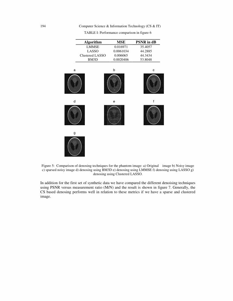
194 Computer Science & Information Technology (CS & IT)
TABLE I: Performance comparison in figure 6
Algorithm MSE PSNR in dB
LMMSE 0.016971 35.4057
LASSO 0.0061034 44.2885
Clustered LASSO 0.006065 44.3434
BM3D 0.0020406 53.8048
Figure 5: Comparison of denosing techniques for the phantom image: a) Original image b) Noisy image
c) sparsed noisy image d) denosing using BM3D e) denosing using LMMSE f) denosing using LASSO g)
denosing using Clustered LASSO.
In addition for the first set of synthetic data we have compared the different denoising techniques
using PSNR versus measurement ratio (M/N) and the result is shown in figure 7. Generally, the
CS based denosing performs well in relation to these metrics if we have a sparse and clustered
image.
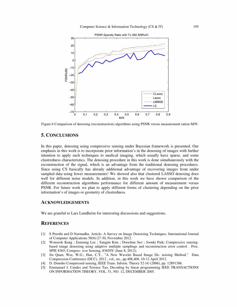
Computer Science & Information Technology (CS & IT) 195
Figure 6 Comparison of denosing (reconstruction) algorithms using PSNR versus measurement ration M/N.
5. CONCLUSIONS
In this paper, denosing using compressive sensing under Bayesian framework is presented. Our
emphasis in this work is to incorporate prior information’s in the denosing of images with further
intention to apply such techniques to medical imaging, which usually have sparse, and some
clustredness characteristics. The denosing procedure in this work is done simultaneously with the
reconstruction of the signal, which is an advantage from the traditional denosing procedures.
Since using CS basically has already additional advantage of recovering images from under
sampled data using fewer measurements! We showed also that clustered LASSO denosing does
well for different noise models. In addition, in this work we have shown comparison of the
different reconstruction algorithms performance for different amount of measurement versus
PSNR. For future work we plan to apply different forms of clustering depending on the prior
information’s of images or geometry of clustredness.
ACKNOWLEDGEMENTS
We are grateful to Lars Lundheim for interesting discussions and suggestions.
REFERENCES
[1] S Preethi and D Narmadha. Article: A Survey on Image Denoising Techniques. International Journal
of Computer Applications 58(6):27-30, November 2012.
[2] Wonseok Kang ; Eunsung Lee ; Sangjin Kim ; Doochun Seo ; Joonki Paik; Compressive sensing-
based image denoising using adaptive multiple samplings and reconstruction error control . Proc.
SPIE 8365, Compres- sive Sensing, 83650Y (June 8, 2012);
[3] Jin Quan; Wee, W.G.; Han, C.Y., ”A New Wavelet Based Image De- noising Method,” Data
Compression Conference (DCC), 2012 , vol., no., pp.408,408, 10-12 April 2012.
[4] D. Donoho Compressed sensing, IEEE Trans. Inform. Theory 52 (4) (2006), pp. 12891306.
[5] Emmanuel J. Candes and Terence Tao, Decoding by linear programming IEEE TRANSACTIONS
ON INFORMATION THEORY, VOL. 51, NO. 12, DECEMBER 2005.
196 Computer Science & Information Technology (CS & IT)
[6] E. Cand‘es, J. Romberg, and T. Tao, Robust uncertainty principles: Ex- act signal reconstruction from
highly incomplete frequency information, IEEE Trans. Inform. Theory, vol. 52, no. 2, pp. 489509,
Feb. 2006.
[7] E. J. Cande‘s and T. Tao, Near-optimal signal recovery from random projections: Universal encoding
strategies?, IEEE Trans. Inf. Theory, vol. 52, pp. 54065425, Dec. 2006.
[8] Michael Lustig and David Donoho and John M. Pauly, Sparse MRI: The Application of Compressed
Sensing for Rapid MR Imaging SPARS’09 Signal Processing with Adaptive Sparse Structured
Representations inria- 00369642, version 1 (2009).
[9] Marcio M. Marim, Elsa D. Angelini, Jean-Christophe Olivo-Marin, A Compressed Sensing Approach
for Biological Microscopy Image Denoising IEEE Transactions 2007.
[10] Wonseok Kang; Eunsung Lee;Eunjung Chea; Katsaggelos, A.K.; Joonki Paik, Compressive sensing-
based image denoising using adaptive multiple sampling and optimal error tolerance Acoustics,
Speech and Signal Processing (ICASSP), 2013 IEEE International Conference on , vol., no.,
pp.2503,2507, 26-31 May 2013.
[11] E.T. Jaynes, Probability Theory, The Logic of Science, Cambridge University Press., ISBN:. 2003.
[12] David J.C. Mackay Information Theory, Inference, and Learning Algorithms, Cambridge University
Press., ISBN: 978-0-521-64298-9, 2003.
[13] Anthony O’Hagen and Jonathan Forster, Kendall’s Advanced Theory of statistics, volume 2B,,
Bayesian Inference, Arnold, a member of the Hodder Headline Group ,ISBN: 0 340 807520, 2004.
[14] James O. Berger Bayesian and Conditional Frequentist Hypothesis Testing and Model Selection, VIII
C:L:A:P:E:M: La Havana, Cuba, November 2001.
[15] Bradley Efron, Modern Science and the Bayesian-Frequentist Controversy; 2005-19B/233, January,
2005.
[16] Michiel Botje R.A.Fisher on Bayes and Bayes’ Theorem ,Bayesian Analysis ,2008.
[17] Elias Moreno and F. Javier Giron, On the Frequentist and Bayesian approaches to hypothesis testing .
January-June 2006,3-28.
[18] Lei Yu, Hong Sun, Jean Pierre Barbot, Gang Zheng, Bayesian Compressive Sensing for clustered
sparse signals IEEE International Conference on Acoustics, Speech and Signal Processing (ICASSP),
2011.
[19] K.J. Friston, W. Penny, C. Phillips, S. Kiebel, G. Hinton, J. Ashburner, Classical and Bayesian
Inference in Neuroimaging: Theory Neuro Image, Volume 16, Issue 2, Pages 465 483 June 2002.
[20] Solomon A. Tesfamicael and Faraz Barzideh, Clustered Compressed Sensing in fMRI Data Analysis
Using a Bayesian Framework, International Journal of Information and Electronics Engineering vol.
4, no. 2, pp. 74-80, 2014.
[21] Dharmpal D. Doye and Sachin D Ruikarh, Wavelet Based Image Denoising Technique, International
Journal of Advanced Computer Science and Applications IJACSA (2011).
[22] Amin Tavakoli and Ali Pourmohammad, Image Denoising Based on Compressed Sensing,
International Journal of Computer Theory and Engineering vol. 4, no. 2, pp. 266-269, 2012.
[23] S. Rangan, A. K. Fletcher, and V. K. Goyal, Asymptotic analysis of MAP estimation via the replica
method and applications to compressed sensing, arXiv:0906.3234v1, 2009.
[24] Mark Schmidt, Least Squares Optimization with L1-Norm Regularization 2005.
[25] Robert Tibshirani, Regression shrinkage and selection via the lasso, In Journal of the Royal Statistical
Society, Series B, volume 58, pages 267288, 1994.
[26] Dabov, K.; Foi, A.; Katkovnik, V.; Egiazarian, K., Image Denoising by Sparse 3-D Transform
Domain Collaborative Filtering Image Processing, IEEE Transactions on , vol.16, no.8, pp.2080,2095,
Aug. 2007.

Computer Science & Information Technology (CS & IT) 197
AUTHORS
Solomon A. Tesfamicael was born in Gonder, Ethiopia in 1973. He received his
Bachelor degree in Mathematics from Bahirdar university, Bahirdar, Ethiopia in 2000
and Master degree in Coding theory from the Norwegian University of Science and
Technology (NTNU) in Trondheim, Norway in 2004. He began his PhD studies in
signal processing sept, 2009 at the department of Electronics and Telecomunications at
NTNU. He is currently working as LECTURER at the Sør-Trondlag university collge
(HiST), in Trondheim, Norway. He has worked as mathematics teacher for secondary schools and as
assistant LECTURER at the Engineering faculity in Bahirdar university in Ethiopia. In addition, he has a
pedagogical studies both in Ethiopia and in Norway. He has authored and co-authtored papers related to
compressed sensing (CS) and multiple input and multiple out put (MIMO) systems. His research interest
are signal processing, Compresses sensing, multiuser communication (MIMO, CDMA), statistical
mechanical methods like replica method, functional magnetic resonance imaging (fMRI) and
mathematical education.
Faraz Barzideh was born in Tehran, Iran in 1987. He received his bachelor degree from
Zanjan University, Zanjan, Iran, in the field of Electronic Engineering in 2011 and
finished his master degree in the field of Medical Signal Processing and Imaging from
Norwegian University of Science and Technology (NTNU) in 2013 and started his PhD
study in University of Stavanger (UiS) in 2014. His research interests are medical signal
and image processing especially in MRI and also compressive sensing and dictionary
learning.

AUTHOR INDEX
Ali M Alshahrani 41
Amartansh Dubey 107
Ana Fernández Vilas 01
Aseem Vyas 117
Ashwathanarayana Shastry 81
Benjamin Aziz 89
Bhurchandi K. M 107
Cédric Sanza 49
Celia Gónzalez Nespereira 01
Chen-Ru Liao 139
Chun-Yi Tsai 25, 139
Dongwei Guo 33
Faheem Ahmed 71
Faraz Barzideh 185
Foudil Cherif 49
Guan-Lin Li 139
Horng-Chang Yang 139
Jia-Shu Wang 139
Jing-Yi Tsai 25
Joseph Fong 165
Kais Dai 01
Kenneth Wong 165
Luiz Fernando Capretz 71
Magdalena Lachor 63
Marcin Michalak 63
Mezati Messaoud 49
Murat Gok 147
Omed Khalind 89
Osman Hilmi Kocal 147
Pin-Syuan Huang 25
Rebeca P. Díaz Redondo 01
Sabu M.K 127
Saiqa Aleem 71
Sevdanur Genc 147
Shasha Wang 33
Siwen Wang 33
Solomon A. Tesfamicae 185
Stuart Walker 41
Tad Gonsalves 157
TakafumiShiozaki 157
Tatiana Ermakova 17
Umesh Rao Hodeghatta 81
Véronique Gaildrat 49
Won-Sook Lee 117
Yan Hong 33
Yu-Fang Wang 25
Zhibo Wei 33