Computer FacilitatedGeneralized CoordinateTransformations of PartialDifferential Equations WithEngineering ApplicationsA. ELKAMEL,1 F.H. BELLAMINE,1,2 V.R. SUBRAMANIAN3

1Department of Chemical Engineering, University of Waterloo, 200 University Avenue West, Waterloo, Ontario,

Canada N2L 3G1

2National Institute of Applied Science and Technology in Tunis, Centre Urbain Nord, B.P. No. 676, 1080 Tunis Cedex,

Tunisia

3Department of Chemical Engineering, Tennessee Technological University, Cookeville, Tennessee 38505

Received 16 February 2008; accepted 2 December 2008

ABSTRACT: Partial differential equations (PDEs) play an important role in describing many physical,

industrial, and biological processes. Their solutions could be considerably facilitated by using appropriate

coordinate transformations. There are many coordinate systems besides the well-known Cartesian, polar, and

spherical coordinates. In this article, we illustrate how to make such transformations using Maple. Such a use has

the advantage of easing the manipulation and derivation of analytical expressions. We illustrate this by

considering a number of engineering problems governed by PDEs in different coordinate systems such as

the bipolar, elliptic cylindrical, and prolate spheroidal. In our opinion, the use of Maple or similar computer

algebraic systems (e.g. Mathematica, Reduce, etc.) will help researchers and students use uncommon

transformations more frequently at the very least for situations where the transformations provide smarter and

easier solutions. �2009 Wiley Periodicals, Inc. Comput Appl Eng Educ 19: 365�376, 2011; View this article online at

wileyonlinelibrary.com; DOI 10.1002/cae.20318

Keywords: partial differential equations; symbolic computation; Maple; coordinate transformations

INTRODUCTION

Partial differential equations (PDEs) are mathematical models

describing physical laws such as chemical processes, electrostatic

distributions, heat flow, and fluid motion. The solution to a number

of PDEs is shaped by the boundaries of the geometry, and thus the

coordinate system selected is influenced by these boundaries. By

choosing a curvilinear coordinate system (�1, �2, �3) such that the

boundary surface is one of the coordinate surfaces, it is possible to

express the solution of the PDE in terms of these new coordinates,

that is, �1, �2, �3. There are many coordinate systems besides the

usual Cartesian, polar, and spherical coordinates. For example,

Figure 1 shows two identical pipes imbedded in a concrete slab. To

find the steady-state temperature, the most suitable coordinate

system is the bipolar coordinate system as will be demonstrated in

more details in Application of the Bipolar Coordinate System

Section. In addition, the separation of variables is a common method

for solving linear PDEs. The separation is different for different

coordinate systems. In other words, we find out in what coordinate

system an equation will be amenable to a separation of variables

solution. The properties of the solution can be related to the

characteristics of the equations and the geometry of the selected

coordinate system. It is possible to prove using the theory of analytic

functions of the complex variable that there are a number of two-

and three-dimensional separable coordinate systems. The coordinate

system is defined by relationships between the rectangular

Correspondence to A. Elkamel (aelkamel@cape.uwaterloo.ca).

� 2009 Wiley Periodicals Inc.

365

coordinates (x, y, z) and the coordinates (�1, �2, �3). The new

coordinate axes are given by the equations �1(x, y, z)¼ constant,

�2(x, y, z)¼ constant, and �3(x, y, z)¼ constant.

For example, polar coordinates are useful for circular

boundaries or ones consisting of two lines meeting at an angle

(see Fig. 2). The families r¼ constant and ’¼ constant are,

respectively, the concentric circles and the radial lines as

illustrated in Figure 2. Coordinate systems more general than

the polar are the elliptic coordinates consisting of ellipses and

hyperbolas. These coordinates are suitable for elliptic boundaries

or ones consisting of hyperbolas as illustrated in Figure 3.

Parabolic cylindrical coordinates, shown in Figure 4, are two

orthogonal families of parabolas, with axes along the x-axis.

These coordinates are suitable, for example, for a boundary

consisting of the negative half of the x-axis. Generally speaking,

the separable coordinate systems for two dimensions consisted of

conic sections; that is, ellipses and hyperbolas or their degenerate

forms (lines, parabolas, circles).

For three dimensions, the separable coordinate systems are

quadratic surfaces or their degenerate forms. A common

coordinate system is the spherical coordinates. The coordinate

surfaces are spheres having centers at the origin, cones having

vertices at the origin, and planes through the z-axis. Robertson’s

condition, which relates scale factors and the properties of

Stackel determinant, places a limit on the number of possible

coordinate systems. Table 1 lists a number of common coordinate

systems. These coordinate systems are: rectangular coordinates,

circular cylindrical coordinates, elliptic cylinder coordinates,

parabolic cylinder coordinates, spherical coordinates, bipolar

coordinates, conical coordinates, parabolic coordinates, prolate

spheroidal coordinates, oblate spheroidal coordinates, ellipsoidal

coordinates, bi-spherical coordinates, and toroidal coordinates.

The names are generally descriptive of the coordinate systems.

For example, the circular cylinder coordinates involve coordinate

surfaces, which are cylinder coaxial. Maple implements,

respectively, about 15 coordinate systems in two dimensions

and 31 in three dimensions.

Let us illustrate one useful application of using these

coordinate systems. For example, if the boundary conditions

require the use of polar coordinates (shown in Fig. 1), the

equation D2’þ k2’¼ 0 (k is a constant), for example, can be split

(making use of Tables 1�3) into two ordinary differential

equations, each for a single independent variable

d2f

dr2þ 1

r

df

drþ 1

r2ðr2k2 � �2Þf ¼ 0;

d2g

d�2þ �2g ¼ 0 ð1Þ

where ’(r, �)¼ f(r)g(�) and � is the separation constant (which

must be integer in the case of polar coordinates since ’ is a

periodic coordinate). We will apply the method of separation of

variables to the PDEs in the examples.

Figure 1 Two identical pipes imbedded in an infinite concrete slab.

Figure 2 Circular cylindrical coordinates. [Color figure can be viewed

in the online issue, which is available at wileyonlinelibrary.com.]

Figure 3 Elliptic cylindrical coordinates. [Color figure can be viewed in

the online issue, which is available at wileyonlinelibrary.com.]

Figure 4 Parabolic coordinates. [Color figure can be viewed in the

online issue, which is available at wileyonlinelibrary.com.]

366 ELKAMEL, BELLAMINE, AND SUBRAMANIAN

So, the basic technique is to transform a given boundary

value problem in the xy plane (or x, y, z space) into a simpler one

in the plane �1�2 (or �1�2�3 space) and then write the solution of

the original problem in terms of the solution obtained for the

simpler equation. This is explained in the next three sections. The

transformations will make the solution more tractable and

convenient to find.

Nowadays, high-performance computers coupled with

highly efficient user-friendly symbolic computation software

tools such as Maple, Mathematica, Matlab, Reduce [htt

p:www.maplesoft.com, http://www. wolfram.com, http://www.

mathworks.com, http://www. reduce-algebra.com] are very useful

in teaching mathematical methods involving tedious algebra and

manipulations. In this paper, the powerful software tool Maple

is used. Maple facilitates the manipulation and derivation of

analytical expressions, and can be used to perform tedious

algebra, complicated integrals, and differential equations [1�3].

A secondary objective of this paper is to expose the student

to different skills in using Maple to perform the algebra and work

with differential equations calculations and solutions in different

coordinate systems.

For the sake of readers not familiar with Maple, a brief

introduction will follow. Maple is a powerful symbolic computa-

tional tool used to perform analytical derivations and numerical

calculations. It is easy to use, and its commands are often

straightforward to know even for a first-time user. In this paper,

the student version of Maple is used. We recommend that the

student uses ‘‘;’’ and not ‘‘:’’ at the end of a command statement

so that Maple prints the results. This helps in fixing mistakes in

the program since the results are printed after every command

statement. In addition, the user might have to manipulate the

resulting expressions from a Maple command to obtain the

equation in the simplest or desired form. All the mathematical

manipulations involved can be performed in the same program,

and Maple can be used to perform all the required steps from

setting up the equations to interpreting plots in the same sheet.

Please note that equations containing ‘‘:¼’’ are results printed by

Maple.

APPLICATION OF THE BIPOLARCOORDINATE SYSTEM

There are a number of real applications for bipolar coordinates

such as pairs of ducts, pipes, transmission lines, and bubbles

[4�9]. We will illustrate the use of the bipolar orthogonal

coordinate system in this section by the following example. Two

identical circular pipes of identical radius R are imbedded in

an infinite concrete slab as shown in Figure 1. The uniform

temperature of both pipes is T0. We want to solve the temperature

distribution in the concrete slab by solving the following

differential Laplace equation:

Table 1 Definition of Common Coordinate Systems

Circular cylindrical (polar)

coordinates (�, �, z)

x¼ � cos�, y¼ � sin�, z

Elliptic cylindrical

coordinates (u, �, z)

x¼ d cosh u cos�, y¼ d sinh u sin�, z

Parabolic cylindrical

coordinates (u, v, z)

x¼ (1/2)(u2�v2), y¼ uv, z

Bipolar coordinates (u, v, z) x ¼ asinh v

cosh v� cos u; y ¼ a

sin u

cosh v� cos u; z

Spherical coordinates (r, �, y) x ¼ r cos� sin �; y ¼ r sin� sin �; z ¼ r cos �

Conical coordinates (�, �, �) x ¼ ���

ab; y ¼ �

a

ffiffiffiffiffiffiffiffiffiffiffiffiffiffiffiffiffiffiffiffiffiffiffiffiffiffiffiffiffiffiffiffiffiffiffiffiffiffið�2 � a2Þð�2 � a2Þ

a2 � b2

r; z ¼ �

b

ffiffiffiffiffiffiffiffiffiffiffiffiffiffiffiffiffiffiffiffiffiffiffiffiffiffiffiffiffiffiffiffiffiffiffiffiffiffið�2 � b2Þð�2 � b2Þ

b2 � a2

r

Parabolic coordinates (u, v, �) x ¼ uvcos�; y ¼ uvsin�; z ¼ 1

2ðu2 � v2Þ

Prolate spheroidal

coordinates (u, v, �)

x ¼ d sinh u sin � cos�; y ¼ d sinh u sin � sin�; z ¼ d cosh u cos �

Oblate spheroidal

coordinates (u, v, �)

x ¼ d cosh u sin � cos�; y ¼ d cosh u sin � sin�; z ¼ d sinh u cos �

Ellipsoidal coordinates

(�1, �2, �3)

x ¼ffiffiffiffiffiffiffiffiffiffiffiffiffiffiffiffiffiffiffiffiffiffiffiffiffiffiffiffiffiffiffiffiffiffiffiffiffiffiffiffiffiffiffiffiffiffiffiffiffiffiffiffiffiffiffið�21 � a2Þð�22 � a2Þð�23 � a2Þ

ða2 � c2Þða2 � b2Þ

s; y ¼

ffiffiffiffiffiffiffiffiffiffiffiffiffiffiffiffiffiffiffiffiffiffiffiffiffiffiffiffiffiffiffiffiffiffiffiffiffiffiffiffiffiffiffiffiffiffiffiffiffiffiffiffiffiffiffið�21 � b2Þð�22 � b2Þð�23 � b2Þ

ðb2 � c2Þðb2 � a2Þ

s;

z ¼ffiffiffiffiffiffiffiffiffiffiffiffiffiffiffiffiffiffiffiffiffiffiffiffiffiffiffiffiffiffiffiffiffiffiffiffiffiffiffiffiffiffiffiffiffiffiffiffiffiffiffiffiffiffið�21 � c2Þð�22 � c2Þð�23 � c2Þ

ðc2 � a2Þðc2 � b2Þ

s

Paraboloidal coordinates

(�1, �2, �3)

x ¼ffiffiffiffiffiffiffiffiffiffiffiffiffiffiffiffiffiffiffiffiffiffiffiffiffiffiffiffiffiffiffiffiffiffiffiffiffiffiffiffiffiffiffiffiffiffiffiffiffiffiffiffiffiffiffið�21 � a2Þð�22 � a2Þð�23 � a2Þ

ða2 � b2Þ

s; y ¼

ffiffiffiffiffiffiffiffiffiffiffiffiffiffiffiffiffiffiffiffiffiffiffiffiffiffiffiffiffiffiffiffiffiffiffiffiffiffiffiffiffiffiffiffiffiffiffiffiffiffiffiffiffiffiffið�21 � b2Þð�22 � b2Þð�23 � b2Þ

ðb2 � a2Þ

s;

z ¼ 1

2ð�21 þ �22 þ �23 � a2 � b2Þ

Bispherical coordinates

(, �, �)

x ¼ a cos�sin

cosh�� cos ; y ¼ a sin�

sin

cosh�� cos ; z ¼ a

sinh�

cosh�� cos

Toroidal coordinates

(, �, �)

x ¼ a cos�sinh�

cosh�� cos ; y ¼ a sin�

sinh�

cosh�� cos ; z ¼ a

sin

cosh�� cos

TRANSFORMATIONS OF PDES 367

> restart: with(student):> eq:¼diff(T(x,y),x$2)þdiff(T(x,y),y$2)¼0;

eq :¼ @2

@x2Tðx; yÞ

� �þ @2

@y2Tðx; yÞ

� �¼ 0

The boundary conditions of this problem dictate the use of

bipolar coordinates (see Fig. 5). According to Table 1, the

following equations define bipolar coordinates:

x ¼ c sinh v

cosh v� cos u; y ¼ c sin u

cosh v� cos uð2Þ

> eq1:¼x�c*sinh(v(x,y))/(cosh(v(x,y))�cos(u(x,y)));

eq1 :¼ x� c sinhðvðx; yÞÞcoshðvðx; yÞÞ � cosðuðx; yÞÞ

> eq2:¼y¼c*sin(u(x,y))/(cosh(v(x,y))�cos(u(x,y)));

eq2 :¼ y ¼ c sinðuðx; yÞÞcoshðvðx; yÞÞ � cosðuðx; yÞÞ

We will show how tractable and convenient it is to solve the

Laplace equation in the bipolar coordinates, whereas in terms of

x, y, and z the temperature field expression is complex. So, the

bipolar coordinates are the ‘‘natural’’ coordinates for this type of

problem.

First of all, we show that the bipolar coordinate system is an

orthogonal coordinate system. This means that the two families

of the coordinate surfaces u(x, y) and v(x, y) are mutually

orthogonal. The lines of intersection of these surfaces constitute

two families of lines. At the point (u, v), we have unit vectors~e1

and ~e2 each, respectively, tangent to the coordinate line of the

bipolar coordinate system which goes through the point. Since the

coordinate system is orthogonal, ~e1 and ~e2 are mutually

perpendicular everywhere

~e1 �~e2 ¼ 0 or1

h1@~r

@u

1

h2@~r

@v¼ 0 ð3Þ

where~r is a position vector and is given by

~r ¼ x~e1 þ y~e2 ð4Þ

Table 2 Scale Factors for Common Coordinate Systems

Circular cylindrical

coordinates (�, �, z)

h1¼ 1, h2¼ �, h3¼ 1

Elliptic cylindrical

coordinates (u, �, z)

h1 ¼ d

ffiffiffiffiffiffiffiffiffiffiffiffiffiffiffiffiffiffiffiffiffiffiffiffiffiffiffiffiffiffiffisinh2 uþ sin2 �

q; h2 ¼ h1; h3 ¼ 1

Parabolic cylindrical

coordinates (u, v, z)

h1 ¼ dffiffiffiffiffiffiffiffiffiffiffiffiffiffiffiu2 þ v2

p; h2 ¼ h1; h3 ¼ 1

Bipolar coordinates (, �, z) h1 ¼ �

cosh�� cos ; h2 ¼ h1; h3 ¼ 1

Spherical coordinate (r, y, �) h1¼1, h2¼ r sin y, h3¼ r

Conical coordinates (�, �, �) h1 ¼ 1; h2 ¼ �

ffiffiffiffiffiffiffiffiffiffiffiffiffiffiffiffiffiffiffiffiffiffiffiffiffiffiffiffiffiffiffiffiffiffiffiffiffiffið�2 � �2Þ

ð�2 � a2Þðb2 � �2Þ

s; h3 ¼ �

ffiffiffiffiffiffiffiffiffiffiffiffiffiffiffiffiffiffiffiffiffiffiffiffiffiffiffiffiffiffiffiffiffiffiffiffiffið�2 � �2Þ

ð�2 � a2Þð�2 � b2Þ

s

Parabolic coordinate (u, v, �) h1 ¼ffiffiffiffiffiffiffiffiffiffiffiffiffiffiffiffi�2 þ �2

p; h2 ¼ h1; h3 ¼ ��

Prolate spheroidal

coordinates (u, v, �)

h1 ¼ dffiffiffiffiffiffiffiffiffiffiffiffiffiffiffiffiffiffiffiffiffiffiffiffiffiffiffiffiffiffisinh2 uþ sin2 �

p; h2 ¼ h1; h3 ¼ d sinh u sin �

Oblate spheroidal

coordinates (u, v, �)

h1 ¼ dffiffiffiffiffiffiffiffiffiffiffiffiffiffiffiffiffiffiffiffiffiffiffiffiffiffiffiffiffiffisinh2 uþ sin2 �

p; h2 ¼ h1; h3 ¼ d cosh u sin �

Ellipsoidal coordinates

(�1, �2, �3)h1 ¼

ffiffiffiffiffiffiffiffiffiffiffiffiffiffiffiffiffiffiffiffiffiffiffiffiffiffiffiffiffiffiffiffiffiffiffiffiffiffiffiffiffiffiffiffiffiffiffiffiffiffiffiffiffiffið�21 � �22Þð�21 � �23Þ

ð�21 � a2Þð�21 � b2Þð�21 � c2Þ

s; h2 ¼

ffiffiffiffiffiffiffiffiffiffiffiffiffiffiffiffiffiffiffiffiffiffiffiffiffiffiffiffiffiffiffiffiffiffiffiffiffiffiffiffiffiffiffiffiffiffiffiffiffiffiffiffiffiffið�22 � �21Þð�22 � �23Þ

ð�22 � a2Þð�22 � b2Þð�22 � c2Þ

s;

h3 ¼ffiffiffiffiffiffiffiffiffiffiffiffiffiffiffiffiffiffiffiffiffiffiffiffiffiffiffiffiffiffiffiffiffiffiffiffiffiffiffiffiffiffiffiffiffiffiffiffiffiffiffiffiffiffi

ð�23 � �21Þð�23 � �22Þð�23 � a2Þð�23 � b2Þð�23 � c2Þ

s

Paraboloidal coordinates

(�1, �2, �3)h1 ¼

ffiffiffiffiffiffiffiffiffiffiffiffiffiffiffiffiffiffiffiffiffiffiffiffiffiffiffiffiffiffiffiffiffiffiffiffiffið�21 � �22Þð�21 � �23Þð�21 � a2Þð�21 � b2Þ

s; h2 ¼

ffiffiffiffiffiffiffiffiffiffiffiffiffiffiffiffiffiffiffiffiffiffiffiffiffiffiffiffiffiffiffiffiffiffiffiffiffið�22 � �21Þð�22 � �23Þð�22 � a2Þð�22 � b2Þ

s;

h3 ¼ffiffiffiffiffiffiffiffiffiffiffiffiffiffiffiffiffiffiffiffiffiffiffiffiffiffiffiffiffiffiffiffiffiffiffiffiffið�23 � �21Þð�23 � �22Þð�23 � a2Þð�23 � b2Þ

s

Bispherical coordinates

(, �, �)h1 ¼ a

ðcosh�� cos Þ sinh� ; h2 ¼ a

ðcosh�� cos Þ sin ;

h3 ¼ a sin

ðcosh�� cos Þ sin�

Toroidal coordinates

(, �, �)

h1 ¼ a

cosh�� cos ; h2 ¼ h1; h3 ¼ a sinh�

cosh�� cos

368 ELKAMEL, BELLAMINE, AND SUBRAMANIAN

h1 and h2 are scale factors for the bipolar coordinates u and v. We

will write about them later on Equation (2) becomes

1

h1h2@x

@u

� �@x

@v

� �þ @y

@u

� �@y

@v

� �� �¼ 0 ð5Þ

Equation (1) is a conformal transformation to x, y from u, v

coordinates. u, uy, vx, and vy are computed using Maple as

follows:

> eq3:¼diff(eq1,x):eq4:¼diff(eq2,x):

vx:¼solve(eq4,diff(v(x,y),x)):eq31:¼simplify(subs(diff(v(x,y),x)¼vx,eq3)): ux:¼solve(eq31,diff(u(x,y),x));

ux :¼ � sinðuðx; yÞÞ sinhðvðx; yÞÞc

> vx:¼simplify(subs(diff(u(x,y),x)¼ux,vx));

� cosðuðx; yÞÞ coshðvðx; yÞÞ � 1

c

> eq5:¼diff(eq1,y):eq6:¼diff(eq2,y):uy:¼solve(eq5,diff(u(x,y),y)):eq61:¼simplify(subs(diff(u(x,y),y)¼uy,eq6)):vy:¼solve(eq61,diff(v(x,y),y));

vy :¼ � sinðuðx; yÞÞ sinhðvðx; yÞÞc

uy:¼simplify(subs(diff(v(x,y),y)¼vy,uy));

uy :¼ cosðuðx; yÞÞ coshðvðx; yÞÞ � 1

c

The Cauchy�Riemann conditions are satisfied since:

simplify(ux�vy);simplify(uyþvx);

0

0

and thus we conclude that the bipolar coordinate system is

orthogonal.

Next, we obtain the scale factors hi (I¼ 1, 2) given by

hi ¼ @~r

@�i

��������; �1 ¼ u and �2 ¼ v ð6Þ

The scale factor hi can be interpreted as follows: a change du

in the bipolar coordinate system produces a displacement h1 du

along the coordinate line. Now, we notice that the rate of

displacement along u due to a displacement along the x-axis is

h1(@u/@x) which is the same as the rate of change of x due to a

displacement h1 du. The same argument goes for the scale factor

h2. The scales of the new coordinates and the change of scale

from point to point determine the important properties of the

coordinate system. The scale factors play a role in expressing the

Table 3 Line and Volume Elements Along With Differential Operators in Curvilinear Orthogonal Coordinate System

Scale factors, hn hn ¼ffiffiffiffiffiffiffiffiffiffiffiffiffiffiffiffiffiffiffiffiffiffiffiffiffiffiffiffiffiffiffiffiffiffiffiffiffiffiffiffiffiffiffiffiffiffiffiffiffiffiffiffiffiffiffi@x

@�n

� �2

þ @y

@�n

� �2

þ @z

@�n

� �2s

¼ffiffiffiffiffiffiffiffiffiffiffiffiffiffiffiffiffiffiffiffiffiffiffiffiffiffiffiffiffiffiffiffiffiffiffiffiffiffiffiffiffiffiffiffiffiffiffiffiffiffiffiffiffiffiffi@�n@x

� �2

þ @�n@y

� �2

þ @�n@z

� �2s24

35�1

Line element, ds ds ¼ffiffiffiffiffiffiffiffiffiffiffiffiffiffiffiffiffih2nðd�nÞ2

q

Volume element, dV dV ¼ h1h2h3d�1d�2d�3

Gradient, r r ¼ 1

h1

@

@�1~e1 þ 1

h2

@

@�2~e2 þ 1

h3

@

@�3~e3

Divergence, r �~A r �~A ¼ 1

h1h2h3

X3n¼1

@

@�1h1h2h3

An

hn

� �

Curl, r�~A r�~A ¼ 1

h1h2h3

Xm;n;p

hm~em@

@�nðhpApÞ � @

@�pðhnAnÞ

� �; m; n; p ¼ 1; 2; 3; or 2; 3; 1 or 3; 1; 2

Laplacian, r2 r2 ¼ 1

h1h2h3

X3n¼1

@

@�n

h1h2h3

h2n

@

@�n

� �

Figure 5 Bipolar coordinates. [Color figure can be viewed in the online

issue, which is available at wileyonlinelibrary.com.]

TRANSFORMATIONS OF PDES 369

differential/integral operators, line, surface, and volume ele-

ments, and for the sake of completeness, they are shown in

Table 2 for common coordinate systems. After some algebraic

manipulations, we find that

> h1square:¼factor(simplify(1/(ux^(2)þuy^(2)))):h[1]:¼simplify(sqrt(h1square),sqrt,symbolic);

h1 :¼ � c

cosðuðx; yÞÞ � coshðvðx; yÞÞSo,

h1 ¼ffiffiffiffiffiffiffiffiffiffiffiffiffiffiffiffiffiffiffiffiffiffiffiffiffiffiffiffiffiffiffiffi@x

@u

� �2

þ @y

@u

� �2s

¼ c

cosh v� cos uð7Þ

> h2square:¼factor(simplify(1/(vx^(2)þvy^(2)))):h[2]:¼simplify(sqrt(h2square),sqrt,symbolic);

h2 :¼ � c

�coshðvðx; yÞÞ þ cosðuðx; yÞÞand so,

h2 ¼ffiffiffiffiffiffiffiffiffiffiffiffiffiffiffiffiffiffiffiffiffiffiffiffiffiffiffiffiffiffiffiffi@x

@v

� �2

þ @y

@v

� �2s

¼ c

cosh v� cos uð8Þ

Next, we need to obtain expressions for the parameter c in

terms of R and L. The y-axis lies in the middle between the two

cylinders, while the x-axis crosses the centers of the cylinders.

After algebraic manipulations, the relationship between the

Cartesian and bipolar coordinates can be expressed as follows:

x2 þ ðy� c cot uÞ2 ¼ c2 csc2 u ð9Þ

ðx� c coth vÞ2 þ y2 ¼ c2 csc h2v ð10ÞThis form of writing the relationship between the ‘‘old’’ set

of coordinates, that is, x, y and the ‘‘new’’ set of coordinates u, v

provides us a further insight since we can notice that Equations

(9) and (10) are circles. For an arbitrary v¼ 0, from Equation

(10) we have a circle of radius c csc hh0 and center (c coth 0, 0).Also, when v¼�0, we have a circle of radius c csc hh0 and

center (�c coth 0, 0). Now, when

c csc h0 ¼ R ð11Þand,

c coth 0 ¼L

2þ R ð12Þ

Then

c ¼ R sinh cosh�1 1þ L

2R

� �� �ð13Þ

The obvious next step is to transform the differential

equation from x, y to u, v coordinates. Using Maple, we can

simply use the Laplacian command. However, Laplace form does

not govern many differential equations, and so we will follow the

approach needed to map a differential equation from a set of

coordinates to another. So, first, we need to get the second

derivatives of u, v with respect to x, y

> uxx:¼diff(ux,x):uxx:¼simplify(subs(diff(u(x,y),x)¼ux,diff(v(x,y),x)¼vx,uxx)):> vxx:¼diff(vx,x):vxx:¼simplify(subs(diff(u(x,y),x)¼ux,diff(v(x,y),x)¼vx,vxx)):> uyy:¼diff(uy,y):uyy:¼simplify(subs(diff(u(x,y),y)¼uy,diff(v(x,y),y)¼vy,uyy)):> vyy:¼diff(vy,y):vyy:¼simplify(subs(diff(u(x,y),y)¼uy,diff(v(x,y),y)¼vy,vyy)):

Then, we map the differential equation into the bipolar

coordinates:

> eq1:¼eval(subs(T(x,y)¼TT(u(x,y),v(x,y)),eq)):eq2:¼subs(diff(v(x,y),y$2)¼�diff(v(x,y),x$2),diff(u(x,y),y$2)¼�diff(u(x,y),x$2),diff(v(x,y),y)¼diff (u(x,y),x),diff(v(x,y),x)¼-diff(u(x,y),y),eq1):eq3:¼factor(expand(eq2)):eq4:¼D[2,2](TT)(u(x,y),v(x,y))þD[1,1](TT)(u(x,y),v(x,y)):eq5:¼subs(u(x,y)¼u,v(x,y)¼v,eq4):Eq:¼convert(eq5,diff);

Eq :¼ @2

@u2TTðu; vÞ

� �þ @2

@v2TTðu; vÞ

� �

which can be rewritten as

@2T

@u2þ @2T

@v2¼ 0 ð14Þ

which shows that Laplace’s equation is invariant under a mapping

to bipolar coordinates. Now, if T changes with respect to z as well,

then the transformed PDE can be shown to be

1

h1h2

@2T

@u2þ @2T

@v2

� �þ @2T

@z2¼ 0 ð15Þ

but since the temperature does not change with respect to z,

that is, @T/@z¼ 0, then Equation (14) is reduced to (13). The

transformed boundary conditions in the u, v coordinates are

T ¼ T1 at v ¼ 0; T ¼ T2 at v ¼ �0 ð16ÞAt this point, we can use the method of separation of

variables covered in many undergraduate and graduate textbooks

[10,11] (so T(u, v)¼X(u)Y(v)). The separation of variables splits

the PDE into two ODEs. We assume that the temperature T(u, v)

is only dependent on v. So, in our particular case, the separation

constant is ln¼ 0. So, we end up solving the following

differential equation with its Dirichlet boundary conditions:

> Eq:¼diff(Y(v),v$2);d2

dv2YðvÞ ¼ 0

> bc1:¼subs(v¼eta[0],Y(v))¼T[1];

bc1 :¼ Yðh0Þ ¼ T1

370 ELKAMEL, BELLAMINE, AND SUBRAMANIAN

> bc2:¼subs(v¼�eta[0], Y(v))¼T[2];

bc2 :¼ Yð�h0Þ ¼ T2

> sol:¼dsolve(Eq,Y(v)):eq1:¼subs(v¼eta[0],Y(eta[0])¼T[1],sol):eq2:¼subs(v¼�eta[0],

Y(�eta[0])¼T[2],sol):eq3:¼solve({eq1,eq2},{_C1,_C2});

and thus:

YðvÞ ¼ ðT1 � T2Þv2h0

þ 1

2T2 þ 1

2T1

which is equal to T(u, v).

Generally, when we conduct the separation of variables, one

gets

> eqs:¼subs(TT(u,v)¼X(u)*Y(v),Eq):eqs:¼expand(eqs):eqs:¼eqs/(X(u)*Y (v)):eqs:¼expand(eqs);

eqs :¼d2

du2XðuÞ

XðuÞ þd2

dv2YðvÞ

YðvÞwe obtain two ODEs in X(u) and Y(v) and the first one is

> eqs1:¼diff(X(u),u$2)þlambda^2*X(u): bc1:¼subs(u¼0,D(X)(u))¼0:bc2:¼subs(u¼Pi,D(X)(u))¼0;

eqs1 :¼ d2

du2� ðuÞ

� �þ �2 � ðuÞ

bc1 :¼ DðXÞð0Þ ¼ 0

bc2 :¼ DðXÞðpÞ ¼ 0

The ODE in X(u) is a regular Sturm�Liouville boundary

value problem [10], with separation constant ln¼ n (where n¼ 1,

2, . . .) with corresponding eigenfunctions Xn(u)¼ sin(nu). The

ODE in Y(v) is

> eqs2:¼diff(Y(v),v$2)�n^2*Y(v);

eqs2 :¼ d2

dv2YðvÞ

� �� n2YðvÞ

> dsolve(eqs2);

YðvÞ ¼ C1 eð�nvÞ þ C2 eðn;vÞ

In order to satisfy the boundary conditions (Eq. 16), we

consider the following solution which is a linear combination of

products, and for which the separation constant is not zero:

Tðu; vÞ ¼ T1 � T2

20vþ T1 þ T2

2

þX1n¼1

ðcnenv þ dne�nvÞ sinðnuÞ

where cn and dn are computed by Maple as follows:

> an:¼(2/Pi)*int(T[1]*sin(n*u),u¼0. . .Pi):bn:¼(2/Pi)*int(T[2]*sin(n*u),u¼0. . .Pi) : assume(n::integer) : assume(n,odd):eval(an):eval(bn): eqc1:¼cn*exp(n*eta[0])þdn*exp(�n*eta[0])¼an:eqc2:¼ cn*exp(�n*eta[0])þdn*exp(n*eta [0])¼bn:solc:¼solve({eqc1,eqc2},{cn,dn});

solc : ¼(cn ¼ 4ð�eð�nþ

0ÞT2 � T1e

ðnþ0Þ

n � eð�nþ0Þ� �2þ eðn�0 Þ

2 ;

dn ¼ 4ð�T1eð�nþ

0Þ � T2e

ðnþ0Þ

n � eð�nþ0Þ� �2þ eðn�0 Þ

� �2 )

where n denotes an odd number (i.e. n¼ 2m�1, m¼ 1, 2. . .).

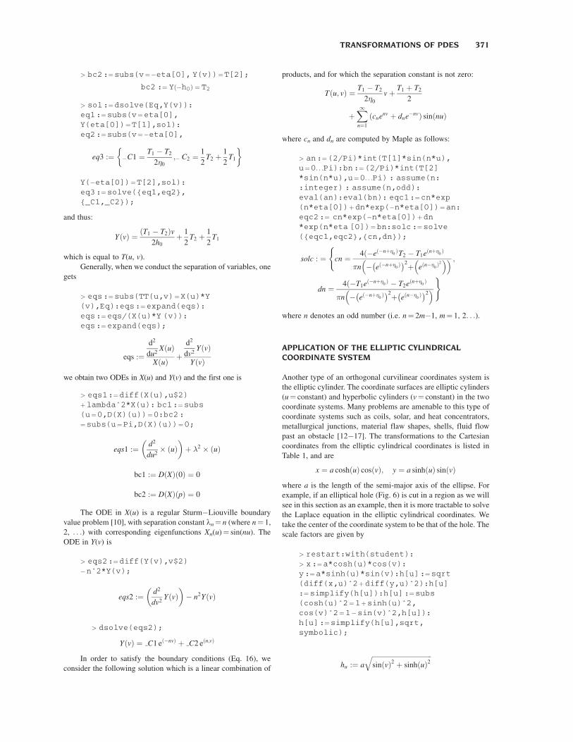
APPLICATION OF THE ELLIPTIC CYLINDRICALCOORDINATE SYSTEM

Another type of an orthogonal curvilinear coordinates system is

the elliptic cylinder. The coordinate surfaces are elliptic cylinders

(u¼ constant) and hyperbolic cylinders (v¼ constant) in the two

coordinate systems. Many problems are amenable to this type of

coordinate systems such as coils, solar, and heat concentrators,

metallurgical junctions, material flaw shapes, shells, fluid flow

past an obstacle [12�17]. The transformations to the Cartesian

coordinates from the elliptic cylindrical coordinates is listed in

Table 1, and are

x ¼ a coshðuÞ cosðvÞ; y ¼ a sinhðuÞ sinðvÞwhere a is the length of the semi-major axis of the ellipse. For

example, if an elliptical hole (Fig. 6) is cut in a region as we will

see in this section as an example, then it is more tractable to solve

the Laplace equation in the elliptic cylindrical coordinates. We

take the center of the coordinate system to be that of the hole. The

scale factors are given by

> restart:with(student):> x:¼a*cosh(u)*cos(v):y:¼a*sinh(u)*sin(v):h[u]:¼sqrt(diff(x,u)^2þdiff(y,u)^2):h[u]:¼simplify(h[u]):h[u]:¼subs(cosh(u)^2¼1þsinh(u)^2,cos(v)^2¼1�sin(v)^2,h[u]):h[u]:¼simplify(h[u],sqrt,symbolic);

hu :¼ a

ffiffiffiffiffiffiffiffiffiffiffiffiffiffiffiffiffiffiffiffiffiffiffiffiffiffiffiffiffiffiffiffiffiffiffiffisinðvÞ2 þ sinhðuÞ2

q

eq3 :¼ �C1 ¼ T1 � T2

20;� C2 ¼ 1

2T2 þ 1

2T1

� �

TRANSFORMATIONS OF PDES 371

Likewise, we obtain hv

hv :¼ a

ffiffiffiffiffiffiffiffiffiffiffiffiffiffiffiffiffiffiffiffiffiffiffiffiffiffiffiffiffiffiffiffiffiffiffiffisinðvÞ2 þ sinhðuÞ2

qThe Laplace equation in elliptic cylindrical coordinates,

assuming a¼ 1, is

> with(linalg):> eq1:¼laplacian(phi(u,v),[u,v],coords¼elliptic):eq1:¼numer(eq1);

eq1 :¼ @2

@u2�ðu; vÞ

� �þ @2

@v2�ðu; vÞ

� �

Using separation of variables, we have �(u, v)¼ �1(u,v)�2(u, v):

> eq2:¼subs(phi(u,v)¼phi[1](u)*phi[2](v),eq1) : eq3:¼expand(eq2):eq4:¼eq3*(1/(phi[1](u)*phi[2](v))):eq4:¼expand(eq4);

eq4 :¼@2

@u2�1ðuÞ

�1ðuÞþ@2

@v2�2ðvÞ

�2ðvÞWe end up with two differential equations for �1(u, v) and

�2(u, v).

eq41:¼diff(phi[1](u),u$2)�p^2*phi[1](u);

eq41 :¼ @2

@u2�1ðuÞ

� �� p2�1ðuÞ

eq42:¼diff(phi[2](v),v$2)þp^2*phi[2](v);

eq42 :¼ @2

@v2�2ðvÞ

� �� p2�2ðvÞ

The two boundary conditions labeled bc1 and bc2 are such

that:

bc1:¼subs(u¼infinity,phi(u,v))¼phi[0]þE[0]*sinh(u)*sin(v);

bc1 :¼ �ð1; vÞ ¼ �0 þ E0 sinhðuÞ sinðvÞbc2:¼subs(u¼u[0],D[ 1](phi)(u,v))¼0;

bc2 :¼ D1ð�Þðu0; vÞ ¼ 0

Assuming that �(u, v)¼A0þA1 sinh u sinvþ A1 cosh sinv,

then enforcing the first boundary condition and since sin-

h u¼ cosh u for large u, we have

eq5:¼phi(u,v)¼_A0þ_A1*sinh(u)*sin(v)þ_A2*cosh(u)*sin(v) : eq6:¼subs(u¼infinity,_A0¼phi[0],eq5):eq7:¼phi[0]þE[0]*sinh(u)*sin(v)¼phi[0]þ(_A1þ_A2)*sinh(u)*sin(v);

eq7 : ¼ �0 þ E0 sinhðuÞ sinðvÞ ¼ �0

þ ð A1þ A2Þ sinhðuÞ sinðvÞWe assume that A0¼E0 which is equal to the potential at

y¼ 0 as shown in Figure 3. The second boundary condition gives

phi(u,v):¼_A0þ_A1*sinh(u)*sin(v)þ_A2*cosh(u)*sin(v):eq8:¼diff(phi(u,v),u):eq8:¼subs(u¼u[0],eq8)¼0;

eq8 : ¼ A1 coshðu0Þ sinðvÞþ A2 sinhðu0Þ sinðvÞ ¼ 0

So, now we can solve for the constants A1 and A2:

eq9:¼solve({eq7, eq8},{_A1,_A2});

eq9 : ¼ A1 ¼ � E0 sinhðu0Þcoshðu0Þ � sinhðu0Þ

�

A2 ¼ coshðu0ÞE0

coshðu0Þ � sinhðu0Þ�

Substituting A1 and A2 in the potential �(u, v), one obtains

eq10:¼subs(_A0¼phi[0],eq5):eq11:¼subs(eq9,eq10);

eq11 : ¼ �0 �E0 sinhðu0Þ sinhðuÞ sinðvÞ

coshðu0Þ � sinhðu0Þþ coshðu0ÞE0 coshðuÞ sinðvÞ

coshðu0Þ � sinhðu0Þ

The electrostatic field E is the gradient of the potential, and

thus is given by

E(u,v):¼�grad(rhs(eq11),[u,v],coords¼elliptic);

Figure 6 The shape of the elliptic hole which is illuminated with the

field E0.

372 ELKAMEL, BELLAMINE, AND SUBRAMANIAN

A field plot is shown Figure 7 reflecting the elliptic

cylindrical coordinate system.

APPLICATION OF THE PROLATESPHEROIDAL COORDINATES

In three dimensions, as shown in Table 1, there are a number of

three-dimensional coordinates. In here, we will give as an

example the case of the prolate spheroidal coordinates system

illustrated in Figure 8. This type of coordinates system has been

used extensively in many fields. For example, raindrops, dust

grains in plasma, molten regions in laser welding, ground rod

connection, conducting electrodes, ventricle, diatomic molecules,

hydrogen molecular ions, and biological cells [11,18�24]

are modeled as prolate spheroidal objects. As an example, the

shape of a football ball is a prolate spheroid. The transformation

to the Cartesian coordinates from the prolate spheroidal

coordinates is listed in Table 1. We will repeat here for the sake

of clarity:

x ¼ d sinhðuÞ sinðvÞ cosð�Þ;y ¼ d sinhðuÞ sinðvÞ sinð�Þ; z ¼ d coshðuÞ cosðwÞ

where d is the focal length for the prolate spheroidal system.

However, we need to be aware that there are other equivalent

transformations. When �¼ cosh(u), ¼ cos v, then one gets

x ¼ d

ffiffiffiffiffiffiffiffiffiffiffiffiffiffiffiffiffiffiffiffiffiffiffiffiffiffiffiffiffiffiffiffiffið�2 � 1Þð1� 2Þ

qcosð�Þ;

y ¼ d

ffiffiffiffiffiffiffiffiffiffiffiffiffiffiffiffiffiffiffiffiffiffiffiffiffiffiffiffiffiffiffiffiffið�2 � 1Þð1� 2Þ

qsinð�Þ; z ¼ d�

where 1� ��1, �1� � 1, 0��� 2p.To compute the volume and surface area in the prolate

spheroidal coordinate system, the Jacobian matrix associated

with the coordinate transformation must be calculated. The

Jacobian matrix elements are the partial derivatives of the

transformation from prolate spherical to Cartesian coordinates.

So, the infinitesimal change in volume is the determinant of the

Jacobian matrix:

restart:with(student):with(linalg):with (PDEtools):T:¼[d*sinh(u)*sin(v)*cos(phi),d*sinh(u)*sin(v)*sin(phi),d*cosh(u)*cos(v)]:J:¼jacobian(T,[u,v,phi]):dV:¼simplify(det(J))*d(u)*d(v)*d(phi);

dV : ¼ d3 sinðvÞ sinhðuÞðcoshðuÞ2

� cosðvÞ2Þ dðuÞ dðvÞ dð�ÞSimilarly, for the computation of surfaces, we need to

compute the two-dimensional Jacobian matrix in the desired

direction.

Eðu; vÞ : ¼ ��E0 sinhðu0Þ coshðuÞ sinðvÞ

coshðu0Þ � sinhðu0Þ þ coshðu0ÞE0 sinhðuÞ sinðvÞcoshðu0Þ � sinhðu0Þffiffiffiffiffiffiffiffiffiffiffiffiffiffiffiffiffiffiffiffiffiffiffiffiffiffiffiffiffiffiffiffiffiffiffiffi

sinhðuÞ2 þ sinðvÞ2q ;

264

�E0 sinhðu0Þ sinhðuÞ cosðvÞcoshðu0Þ � sinhðu0Þ þ coshðu0ÞE0 coshðuÞ cosðvÞ

coshðu0Þ � sinhðu0ÞffiffiffiffiffiffiffiffiffiffiffiffiffiffiffiffiffiffiffiffiffiffiffiffiffiffiffiffiffiffiffiffiffiffiffiffisinhðuÞ2 þ sinðvÞ2

q �

Figure 7 Field plot of E(u, v/E0) which reflects the elliptic coordinate

system.

Figure 8 Prolate spherical coordinates. [Color figure can be viewed in

the online issue, which is available at wileyonlinelibrary.com.]

TRANSFORMATIONS OF PDES 373

In this section, we want to obtain an expression for the

equilibrium temperature distribution of a metal spheroid. Let us

suppose that because of an internal heating system within the

spheroid (�¼ �i), its surface temperature is

� ¼ 10þ 30 cos2

The prolate spheroid made of metal is immersed in a large

container filled with insulating powder. The ambient temperature

is 208C. So, basically, we need to solve for the Laplace equation

in prolate spheroidal coordinates:

eq1:¼laplacian(psi(xi,eta,phi),[xi,eta,phi],coords¼prolatespheroidal(a)):eq2:¼expand(eq1):

eq2 :¼cothð�Þ @

@�cð�; ; �Þ

a2ðsinhð�Þ2 þ sinðÞ2Þ

þ@2

@�2cð�; ; �Þ

a2ðsinhð�Þ2 þ sinðÞ2Þ

þcotðÞ @

@cð�; ; �Þ

a2ðsinhð�Þ2 þ sinðÞ2Þ þ@2

@2cð�; ; �Þ

a2ðsinhð�Þ2 þ sinðÞ2Þ

þ@2

@�2cð�; ; �Þ

a2ðsinhð�Þ2 þ sinðÞ2Þ sinðÞ2 sinhð�Þ2

The system of prolate spheroidal coordinate is separable. So

writing the dependent variable C(�, , �) as the product of threefunctions X(�)H()F(�) will split the Laplacian equation in three

ordinary differential equations:

eq3:¼subs(psi(xi,eta,phi)¼Xi(xi)*Eta(eta)*Phi(phi),eq2):eq4:¼eq3*(1/(Xi(xi)*Eta(eta)*Phi(phi))):eq4:¼expand(eq4):eq4:¼expand(a^2*eq4);

The three differential equations are:

ode1 :¼ @2

@�2Fð�Þ

� �þ q2Fð�Þ ¼ 0

eq42 :¼ @2

@2HðÞ

� �þ cotðÞ @

@HðÞ

� �

þ pðpþ 1Þ þ q2

sinðÞ2 !

HðÞ ¼ 0

eq43 :¼ @2

@�2Xð�Þ

� �þ cothð�Þ @

@�Xð�Þ

� �

� pðpþ 1Þ þ q2

sinhð�Þ2 !

Xð�Þ ¼ 0

q and p are the introduced separation variables. The differential

equations in H() and X(�) are transformed using the following

change of variables:

lð�Þ :¼ coshð�Þ

mðÞ :¼ cosðÞThen, we will get the following differential equations:

eq430:¼changevar(Xi(xi)¼f(lambda(xi)),eq43):eq431:¼numer(simplify(subs(lambda(xi)¼cosh(xi),eq430))):eq432:¼subs(cosh(xi)¼lambda,eq431):eq432:¼convert(eq432,diff):eq432a:¼collect(eq432,diff(f(lambda),lambda$2)):eq432b:¼collect(eq432,diff(f(lambda),lambda)):eq432c:¼collect(eq432,f(lambda)):a:¼factor(1þlambda^4�2*lambda^2):b:¼factor(2*lambda^3�2*lambda):fac:¼1�lambda^2:a1:¼simplify(a/fac):b1:¼simplify(b/fac):c:¼simplify((p^2*lambda^2�p^2þp*lambda^2�p�q^2)/fac):c1:¼collect(c,p^2):ode3:¼a1*diff(f(lambda),lambda$2)þb1*diff(f(lambda),lambda)þc1*f(lambda);

ode3 :¼ ð1� l2Þ @2

@l2f ðlÞ

� �

�2l@

@lf ðlÞ

� �þ pðpþ 1Þ þ q2

l2 � 1

� �f ðlÞ

and the same Maple technique is used for the equation in H(),

ode2 :¼ ð1� m2Þ @2

@m2gðmÞ

� �� 2m

@

@mgðmÞ

� �

þ pðpþ 1Þ þ q2

m2 � 1

� �gðmÞ

So, we need to solve the differential equations labeled above

by ode1, ode2, and ode3. We rename, respectively, f and g to X(�)and H().

Phi:¼rhs(dsolve(ode1,Phi(phi)));alias(P¼LegendreP,Q¼LegendreQ):f:¼rhs(dsolve(ode3,f(lambda)));g:¼rhs(dsolve(ode2,g(mu))):Xi:¼subs(lambda¼cosh(xi),f):Eta:¼subs(mu¼cos(eta),g);

F :¼ C1 sinðq�Þ þ C2 cosðq�ÞX :¼ C1Qðp; q; coshð�ÞÞ þ C2 Pðp; q; coshð�ÞÞH :¼ C1 Pðp; q; cosðÞÞ þ C2Qðp; q; cosðÞÞ

where _C1 and _C2 are constants. We notice that both X(�) andH() solutions are functions of associated Legendre functions of

the first and second kind.

The solution C(�, , �) has axial symmetry about the z-axis

and so it is independent of � and is given by C(�, ,

�)¼X(�)H(). Let the boundary conditions be C(�, �0,)¼M()¼ 10þ 30 cos2 , and hence m¼ cos ranges only

374 ELKAMEL, BELLAMINE, AND SUBRAMANIAN

between �1 and 1. The associated Legendre functions of

the second kind Qn(cos ) are unbounded for m¼ 1, and so the

solution C(�, ) depends only on the associated Legendre

functions of the first kind illustrated in Figure 9 and has the form

Pn(cos )Pn(cosh �), in other words:

N:¼infinity;Psi(xi):¼sum(’A[i]*P(i,mu)*(P(i,cosh(mu))/P(i,cosh(xi0)))’,’i’¼0. . .N);

Cð�Þ :¼X1i¼0

Ai Pði;mÞPði; coshð�ÞÞPði; coshð�0ÞÞ

Enforcing the boundary condition that C(�, �0, )¼M(),one obtains

Psi(xi):¼sum(’A[i]*P(i,mu)*(P(i,cosh(xi))/P(i,cosh(xi0)))’,’i’¼0. . .N):M(mu):¼subs(xi¼xi0,Psi(xi));

MðmÞ :¼X1i¼0

AiPði;mÞ

But, when we truncate N to 5,

MðmÞ : ¼ A0 þ A1mþ A2Pð2;mÞ þ A3Pð3;mÞþ A4Pð4;mÞ þ A5Pð5;mÞ

and so to compute An, we will have to perform the following

computation:

An ¼ nþ 1

2

� �Z 1

�1

MðmÞPnðmÞ dm

> for i from 0 to 10 do A[i]¼evalf((iþ0.5)*int((10þ30*mu^2)*P(i,mu),mu¼-1. . .1)); od;

A0 ¼ 20:0;A1 ¼ 0;A2 ¼ 20:00000000

þ0:1;A3 ¼ 0þ 0:1; A4 ¼ �0:450� 10�11

þ0:1;A5 ¼ 0þ 0:1

Then, substituting the coefficients An into the solution C(�,), one gets

sol1:¼subs(A[0]¼20,A[2]¼20,A[1]¼0,A[3]¼0,A[5]¼0,A[4]¼0,mu¼cos(eta),Psi(xi));

sol1 :¼ 20þ 20Pð2; cosðÞÞPð2; coshð�ÞÞPð2; coshð�0ÞÞ

whose solution C(�, ) is illustrated in Figure 10 for �¼ 2.

CONCLUSION

In this paper, examples of solving problems in coordinate systems

other than the most famous Cartesian, polar, and spherical

coordinates are given. In this article, we gave examples in the

two-dimensional bipolar and elliptic cylindrical coordinates, and

the three-dimensional prolate spheroidal coordinates. Maple

proved to be very useful tool to perform the required trans-

formations from one coordinate system to another, to simplify

expressions, to manipulate the mathematical expressions, and to

plot the solutions. The techniques used in this paper apply to other

coordinate systems such as the parabolic cylindrical coordinates,

conical coordinates, parabolic coordinates, oblate spheroidal

coordinates, ellipsoidal coordinates, bispherical coordinates, and

toroidal coordinates. The boundaries involved in solving the PDE

provide us with the clue of the coordinate system to be used.

Transforming the PDE to one of these coordinates makes the

solution more tractable. For example, we saw that for the case of

boundaries consisting of two circles, the most appropriate

coordinate system to use is the bipolar coordinates. The

aforementioned coordinates are the most commonly used because

they are separable coordinates. In other words, the method of

separation of variables can be used to solve the PDE. However,

Figure 9 Legendre polynomials of the first kind P0(x) . . . P4(x).

[Color figure can be viewed in the online issue, which is available at

wileyonlinelibrary.com.]

Figure 10 Temperature �ðÞ for � ¼ 2.

TRANSFORMATIONS OF PDES 375

one needs to be aware that there are other coordinate systems such

as the hyperbolodoidal, the exponential, and the three-dimen-

sional bipolar coordinates, which are not considered as separable

coordinates, and they are currently the focus of our endeavors.

REFERENCES

[1] V. R. Subramanian, Computer facilitated mathematical methods

in chemical engineering-similarity solution, Chem Eng Educ 40

(2006), 307�312.

[2] D. Richards, Advanced mathematical methods with Maple, Cam-

bridge University Press, Cambridge, 2002.

[3] F. H. Bellame and F. Fgaier, Computer facilitated mathematical

techniques of differential equations governing engineering

processes, World Rev Sci Technol Sust Dev, 5 (2008), 234�252.

[4] J. T. Chen, M. H. Tsai, and C. S. Liu, Conformal mapping and

bipolar coordinate for eccentric Laplace problems, Comput Appl

Eng Educ (accepted).

[5] H. H. Wei, H. Fujioka, and R. B. Hirschl. A model of flow and

surfactant transport in an oscillatory alveolus partially filled with

liquid, Phys Fluids 17 (2005), 1�16.

[6] R. Scharstein and A. M. Davis, Matched asymptotic expansion for

the low-frequency scattering by a semi-circular trough in a ground

plane, IEEE Trans APS 48 (2000), 801�811.

[7] D. W. Pepper and R. E. Cooper, Numerical solution of natural

convection in eccentric annuli, AIAA J 21 (1983), 1331�1337.

[8] M. S. Mokheimer and M. A. El-Shaarawi, Critical values of Gr/Re

for mixed convection in vertical eccentric annuli wit isothermal/

adiabatic walls, J Heat Transf 126 (2004), 479�482.

[9] S. C. Hill and J. M. Jarem, Scattering of multilayer concentric

elliptical cylinders excited by single mode source, PIERS 55 (2005),

209�226.

[10] E. Kreyszig, Advanced engineering mathematics, John Wiley &

Science, New Jersey, 2006.

[11] H. Zahed, J. Mahmoudi, and S. Sobhanian, Analytical study of

spheroidal dusty grains in plasma, Phys Plasmas 13 (2006),

053505�053505�6.

[12] R. H. Jackson, Off-axis expansion solution of Laplace’s equation:

Application to accurate and rapid calculation of coil magnetic

fields, IEEE Trans Electron Dev 46 (1999), 1050�1062.

[13] L. A. Feldman, et al. Initiation of mode I degradation in sodium-beta

alumina electrolytes, J Mater Sci 17 (1982), 517�524.

[14] K. Modenesi, et al. A CFD model for pollutant dispersion in rivers,

Braz J Chem Eng 21 (2004), 557�568.

[15] S. H. Lee and L. G. Leal, Low-Reynolds-number flow past

cylindrical bodies of arbitrary cross-sectional shape, J Fluid Mech

164(1986), 401�427.

[16] B. Podobedov and S. Krinsky, Transverse impedance of elliptical

cross-section tapers, Proceedings of EPACS, 2006, pp 2973�2975.

[17] A. Varma and M. Morbidelli, Mathematical methods in chemical

engineering, Oxford University Press, New York, 1997.

[18] K. Aydin and Y. M. Lure, Millimeter wave scattering and

propagation in rain: A computational study at 94 GHz and 140

GHz for oblate spheroidal and spherical raindrops, IEEE Trans

Geosci Remote Sensing 29 (1991), 593�601.

[19] B. Feng, A. Sitek, and G. T. Gullberg, The prolate spheroidal trans-

form for gated SPECT, IEEE Trans Nucl Sci 43(2001), 872�875.

[20] H. F. Bauer, Steady conduction of heat in prolate spheroidal

systems, J Therm Anal 35(1989), 1571�1602.

[21] T. Kotnik and D. Miklavcic, Analytical description of trans-

membrane voltage induced by electric fields on spheroidal cells,

Biophys J 79 (2000), 670�679.

[22] N. Postacioglu, P. Kapadia, and J. Dowden, A mathematical model

of heat conduction in a prolate spheroidal coordinate system with

applications to the theory of welding, J Phys DAppl Phys 26 (1993),

563�573.

[23] A. de Lima and S. A. Nebram, Theoretical study of intermittent

drying (tempering) in prolate spheroidal bodies, Drying Technol 19

(2001), 1569�1589.

[24] S. McDowell. Using Maple to obtain analytic expressions in

physical chemistry, J Chem Educ 74(1997), 1491� 1493.

BIOGRAPHIES

Ali Elkamel is a professor of Chemical

Engineering at the University of Waterloo.

He holds a BS in Chemical Engineering and a

BS in Mathematics from Colorado School of

Mines, an MS in Chemical Engineering from

the University of Colorado-Boulder, and a PhD

in Chemical Engineering from Purdue Uni-

versity. The goal of his research program is to

develop theory and applications for PSE. The

applications focus on energy production planning, pollution preven-

tion, and product and process design. He is also interested in

integrating computing and process systems engineering in chemical

engineering education. Prior to joining the University of Waterloo, he

served at Purdue University (Indiana), P&G (Italy), Kuwait

University, and the University of Wisconsin-Madison. He has

contributed more than 200 publications in refereed journals and

international conference proceedings.

Fethi Bellamine is a professor at University

November 7, Institute of Applied Science and

Technologies, Tunis, Tunisia. He holds BS,

MS, and PhD degrees in Electrical Engineering

from Colorado State and University of Colo-

rado at Boulder, respectively. From 1995 to

2002, he served as a senior development

engineer for Lucent Technologies, Alcatel

Networks, and NESA. His research interests

are in the areas of modeling and simulation, numerical methods, and

soft computing.

Dr. Venkat Subramanian is an associate

professor in the Department of Chemical

Engineering at the Tennessee Technological

University. He received a BS degree in

chemical and electrochemical engineering

from the Central Electrochemical Research

Institute in India and he received his PhD

degree in Chemical Engineering from the

University of South Carolina. His research

interests include energy systems engineering, multiscale simulation

and design of energetic materials, nonlinear model predictive control,

batteries and fuel cells. He is the principal investigator of the

Modeling, Analysis and Process-Control Laboratory for Electro-

chemical Systems (MAPLE Lab, http://iweb.tntech.edu/

vsubramanian).

376 ELKAMEL, BELLAMINE, AND SUBRAMANIAN