computational photography: image registration jinxiang chai
Post on 22-Dec-2015
225 views
TRANSCRIPT

Computational Photography: Image Registration
Jinxiang Chai
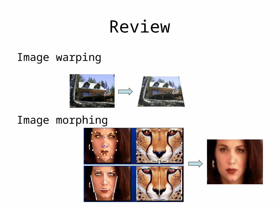
Review
Image warping
Image morphing
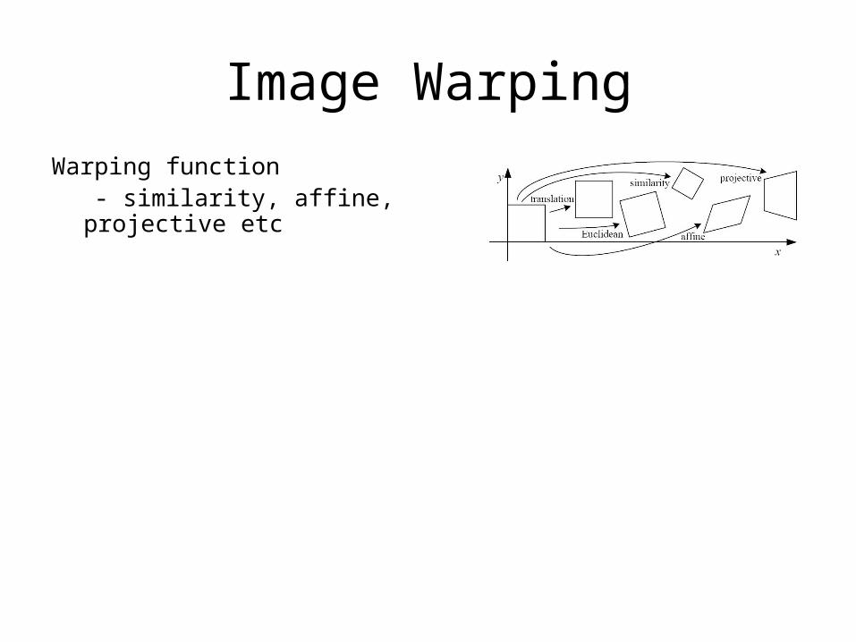
Image Warping
Warping function - similarity, affine, projective etc

Image Warping
Warping function - similarity, affine, projective etc
Image warping - forward warping and two-pass 1D
warping - backward warping
xy
uv
S(x,y) T(u,v)forward
Inverse

Image Warping
Warping function - similarity, affine, projective etc
Image warping - forward warping and two-pass 1D
warping - backward warping
Resampling filter - point sampling - bilinear filter
xy
uv
S(x,y) T(u,v)forward
Inverse
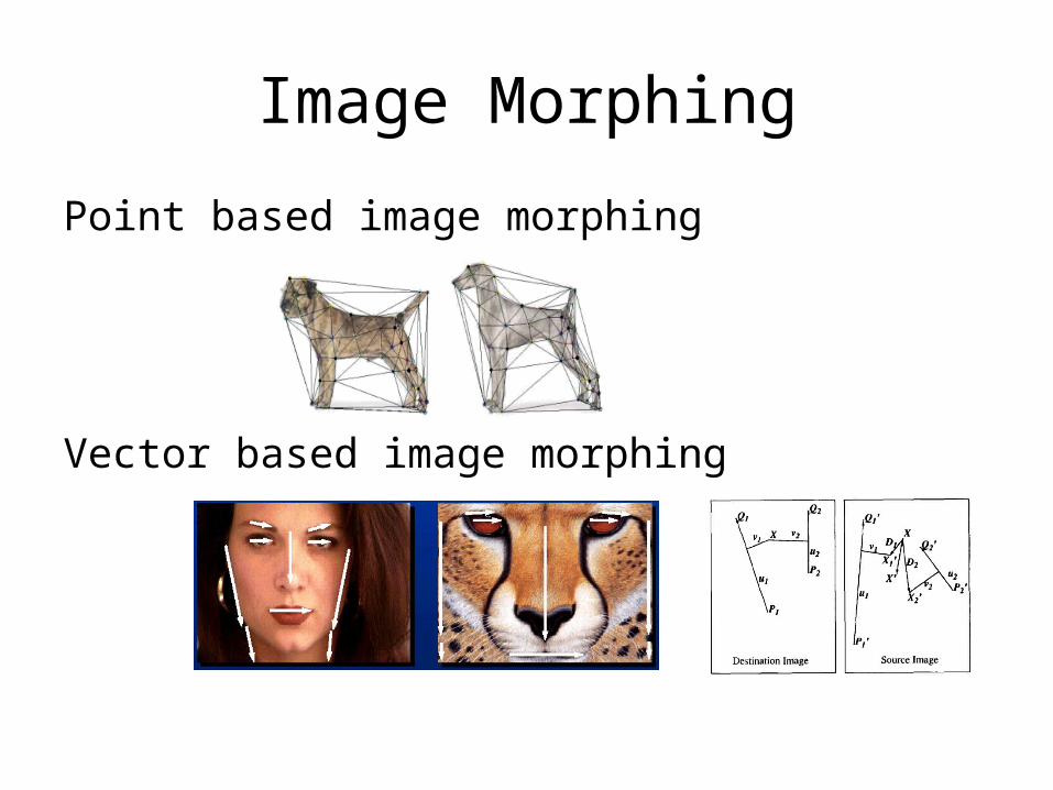
Image Morphing
Point based image morphing
Vector based image morphing
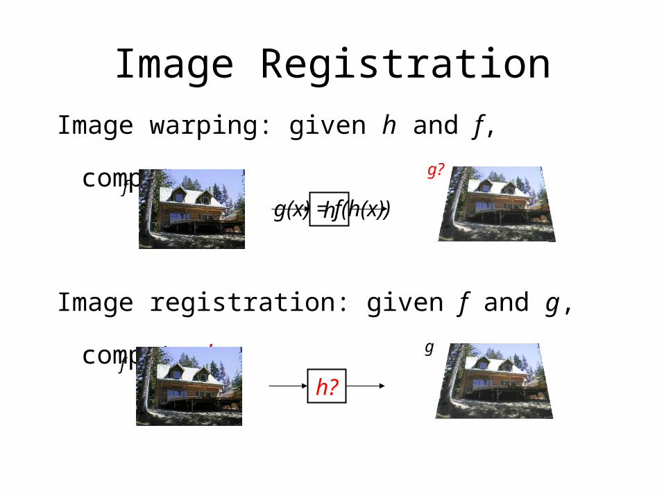
Image RegistrationImage warping: given h and f, compute g
g(x) = f(h(x))
hf
g?
Image registration: given f and g, compute h
h?f
g
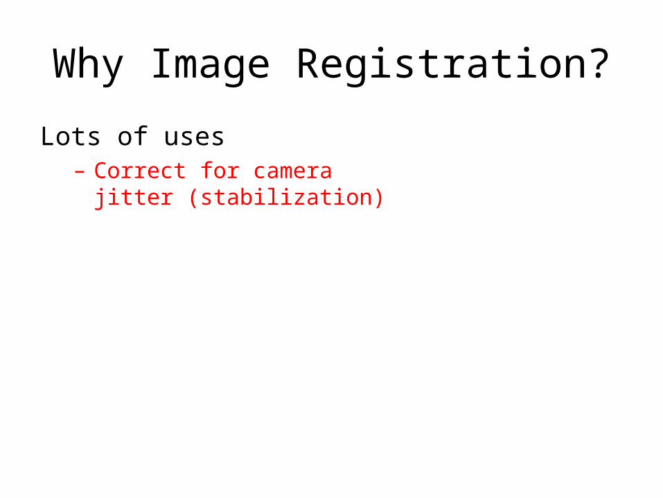
Why Image Registration?
Lots of uses– Correct for camera jitter
(stabilization)
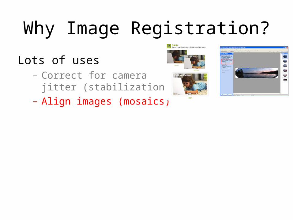
Why Image Registration?
Lots of uses– Correct for camera jitter
(stabilization)– Align images (mosaics)
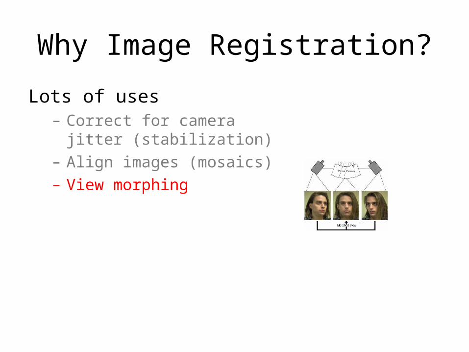
Why Image Registration?
Lots of uses– Correct for camera jitter
(stabilization)– Align images (mosaics)– View morphing
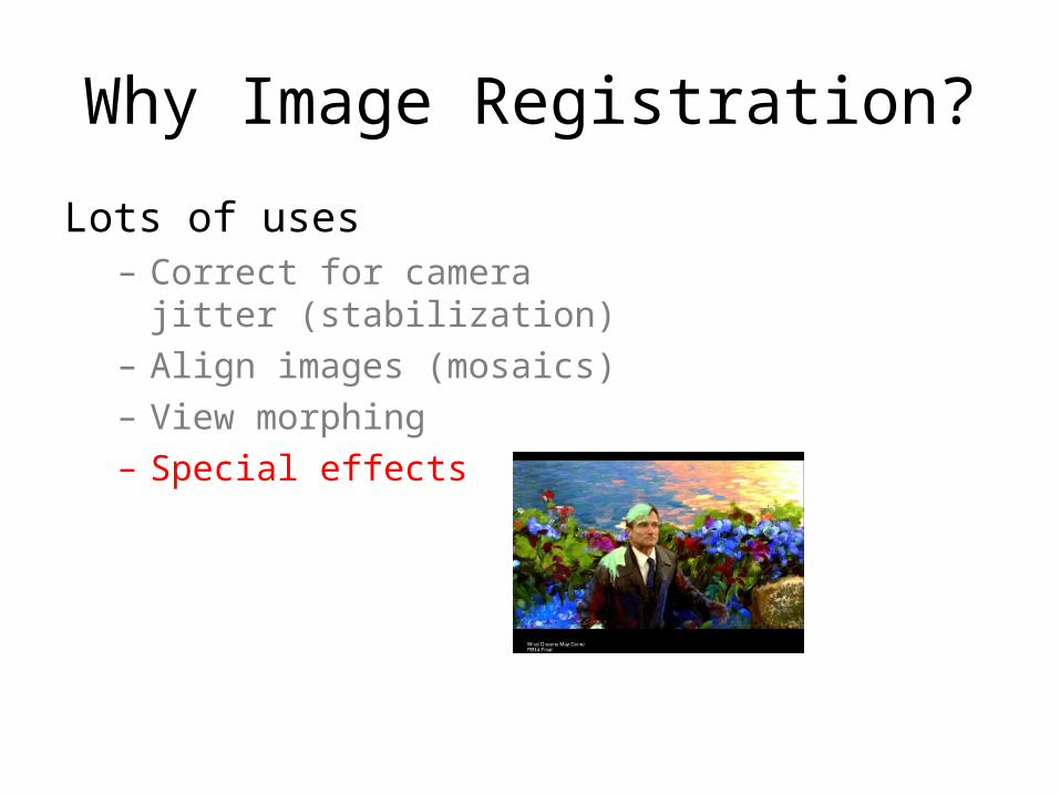
Why Image Registration?
Lots of uses– Correct for camera jitter
(stabilization)– Align images (mosaics)– View morphing– Special effects
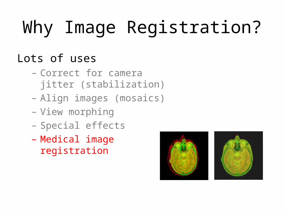
Why Image Registration?
Lots of uses– Correct for camera jitter
(stabilization)– Align images (mosaics)– View morphing– Special effects– Medical image registration
Why Image Registration?
Lots of uses– Correct for camera jitter
(stabilization)– Align images (mosaics)– View morphing– Special effects– Medical image registration– Image based modeling/rendering– Etc.
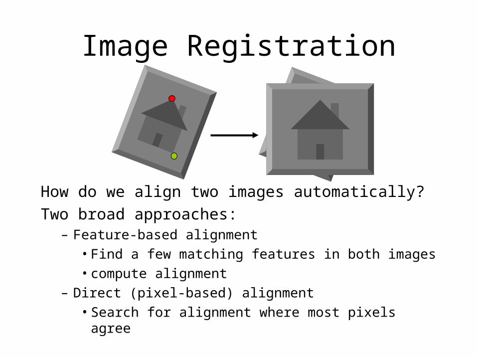
Image Registration
How do we align two images automatically?
Two broad approaches:– Feature-based alignment
• Find a few matching features in both images• compute alignment
– Direct (pixel-based) alignment• Search for alignment where most pixels agree
Outline
Image registration
- feature-based approach
- pixel-based approach
Required Readings
• Section 6.1 (Szeliski book)
• Section 8.1.3 (Szeliski book)
• Section 8.2 (Szeliski book)
• Section 8.4 (Szeliski book)
Outline
Image registration
- feature-based approach
- pixel-based approach
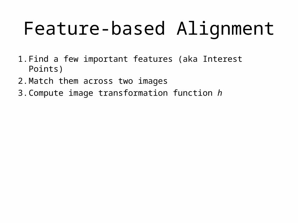
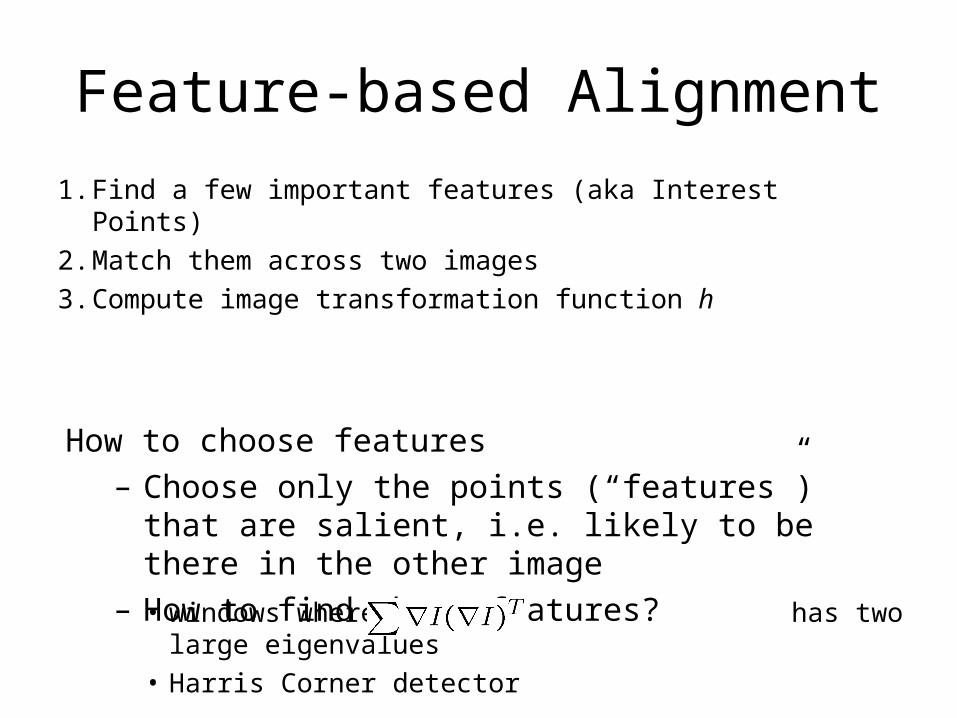
Feature-based Alignment
1. Find a few important features (aka Interest Points)
2. Match them across two images
3. Compute image transformation function h
Feature-based Alignment
1. Find a few important features (aka Interest Points)
2. Match them across two images
3. Compute image transformation function h
How to choose features – Choose only the points (“features”) that are
salient, i.e. likely to be there in the other image– How to find these features?
Feature-based Alignment
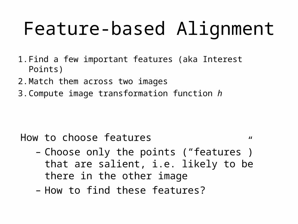
1. Find a few important features (aka Interest Points)
2. Match them across two images
3. Compute image transformation function h
How to choose features – Choose only the points (“features”) that are
salient, i.e. likely to be there in the other image– How to find these features?
• windows where has two large eigenvalues• Harris Corner detector
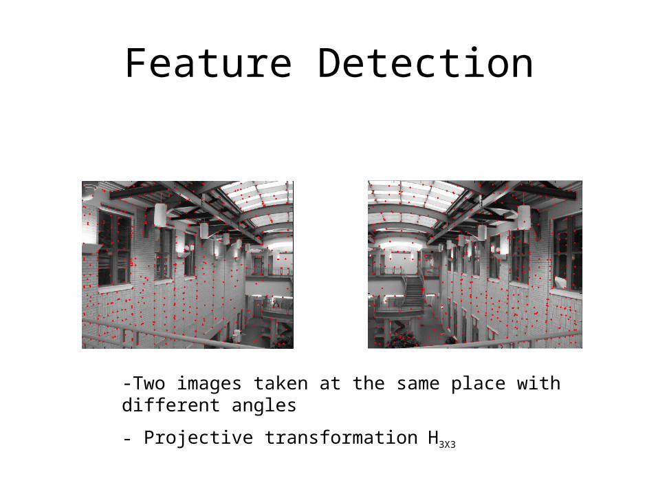
Feature Detection
-Two images taken at the same place with different angles
- Projective transformation H3X3

Feature Matching
?
-Two images taken at the same place with different angles
- Projective transformation H3X3
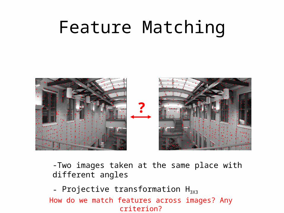
Feature Matching
?
-Two images taken at the same place with different angles
- Projective transformation H3X3
How do we match features across images? Any criterion?

Feature Matching
?
-Two images taken at the same place with different angles
- Projective transformation H3X3
How do we match features across images? Any criterion?
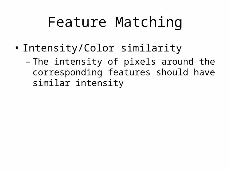
Feature Matching
• Intensity/Color similarity– The intensity of pixels around the
corresponding features should have similar intensity
Feature Matching
• Intensity/Color similarity– The intensity of pixels around the
corresponding features should have similar intensity
– Cross-correlation, SSD
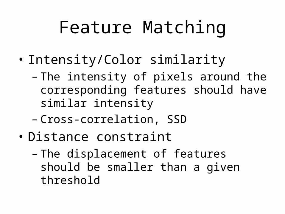
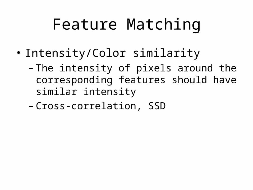
Feature Matching
• Intensity/Color similarity– The intensity of pixels around the
corresponding features should have similar intensity
– Cross-correlation, SSD
• Distance constraint– The displacement of features should be
smaller than a given threshold

Feature-space Outlier Rejection
bad
Good
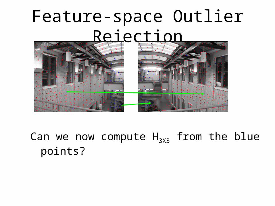
Feature-space Outlier Rejection
Can we now compute H3X3 from the blue points?
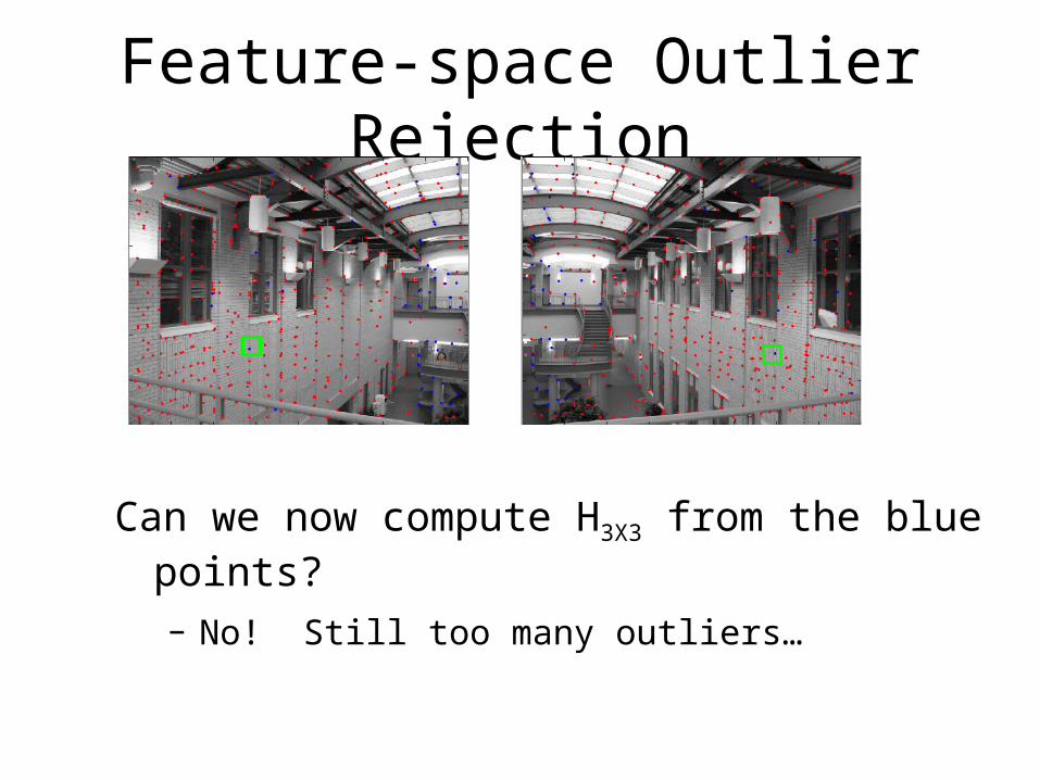
Feature-space Outlier Rejection
Can we now compute H3X3 from the blue points?
– No! Still too many outliers…
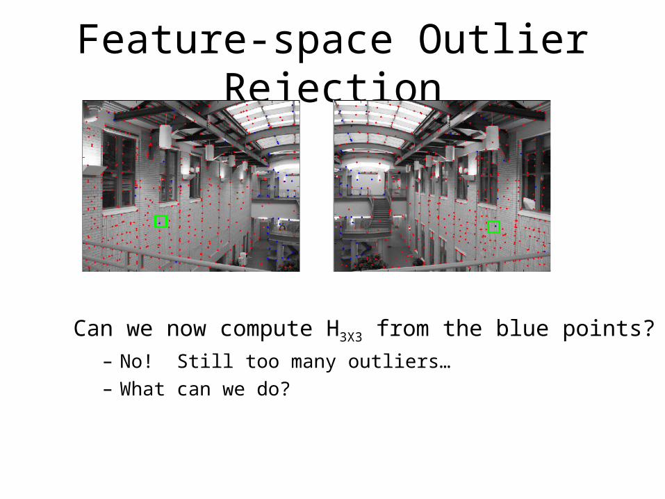
Feature-space Outlier Rejection
Can we now compute H3X3 from the blue points?– No! Still too many outliers… – What can we do?
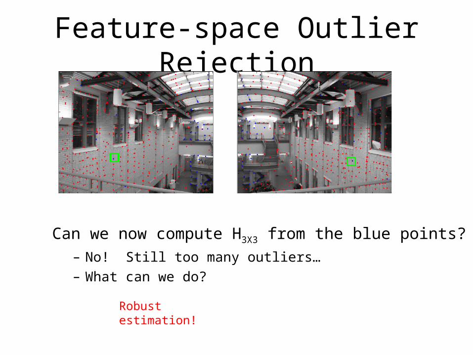
Feature-space Outlier Rejection
Can we now compute H3X3 from the blue points?– No! Still too many outliers… – What can we do?
Robust estimation!

Robust Estimation: A Toy Example
How to fit a line based on a set of 2D points?
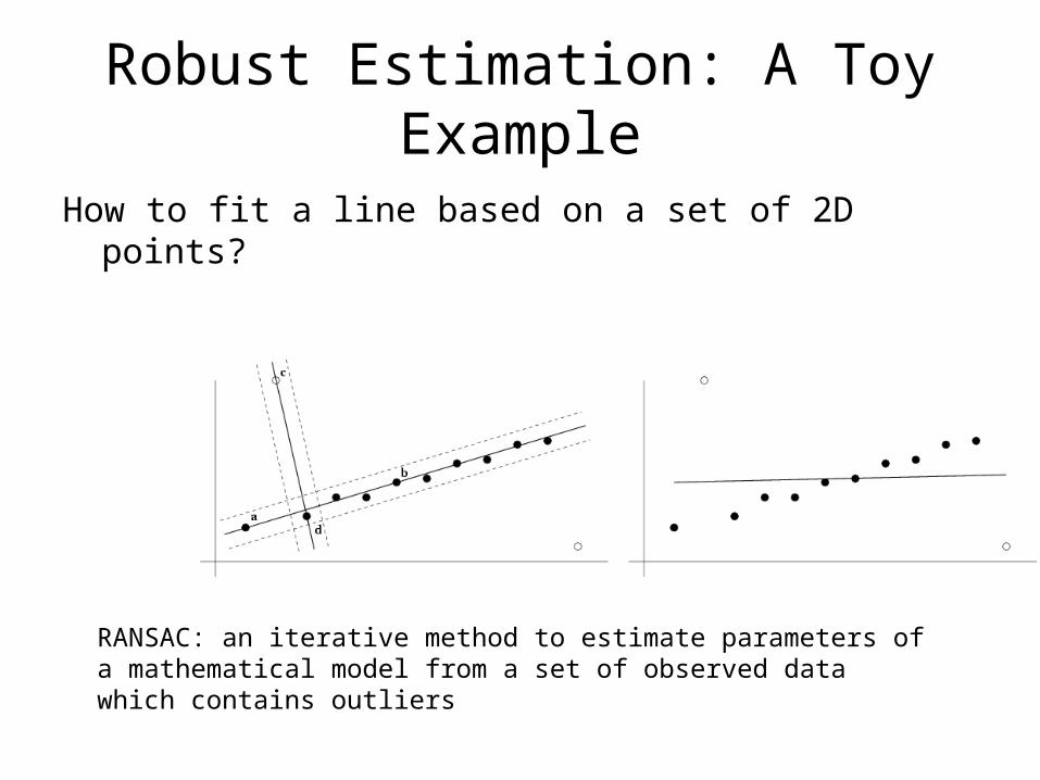
Robust Estimation: A Toy Example
How to fit a line based on a set of 2D points?
RANSAC: an iterative method to estimate parameters of a mathematical model from a set of observed data which contains outliers
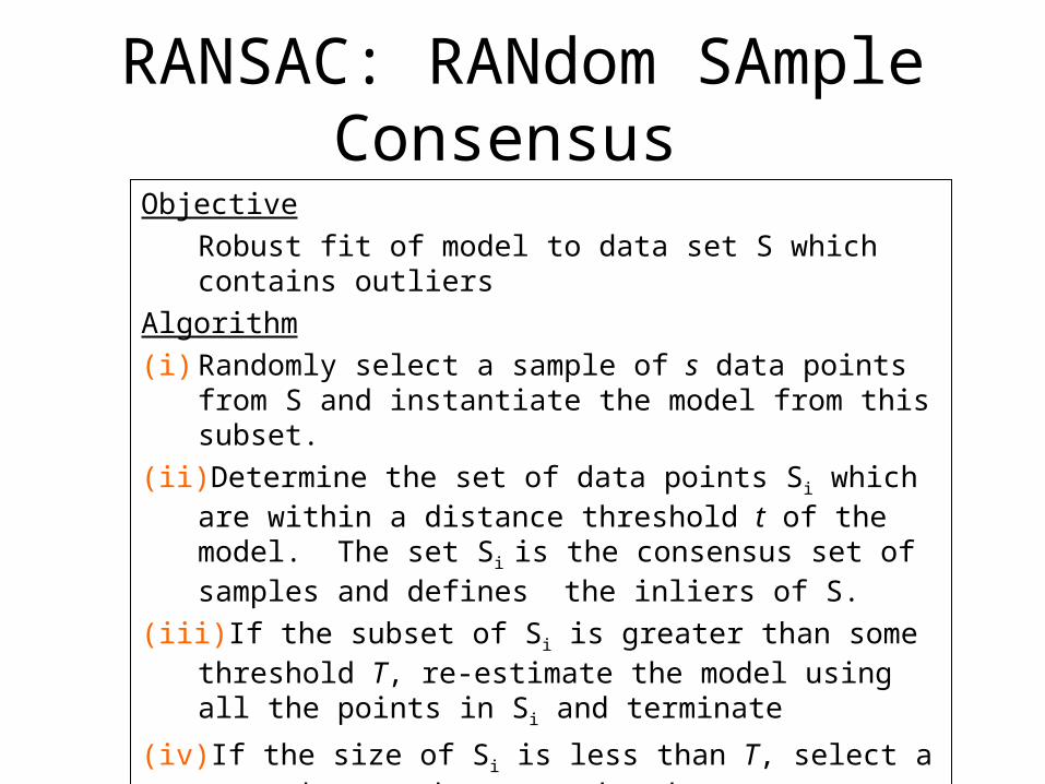
RANSAC: RANdom SAmple Consensus
ObjectiveRobust fit of model to data set S which contains outliers
Algorithm
(i) Randomly select a sample of s data points from S and instantiate the model from this subset.
(ii) Determine the set of data points Si which are within a distance threshold t of the model. The set Si is the consensus set of samples and defines the inliers of S.
(iii) If the subset of Si is greater than some threshold T, re-estimate the model using all the points in Si and terminate
(iv) If the size of Si is less than T, select a new subset and repeat the above.
(v) After N trials the largest consensus set Si is selected, and the model is re-estimated using all the points in the subset Si

RANSAC
Repeat M times:– Sample minimal number of matches to
estimate two view relation (affine, perspective, etc).
– Calculate number of inliers or posterior likelihood for relation.
– Choose relation to maximize number of inliers.

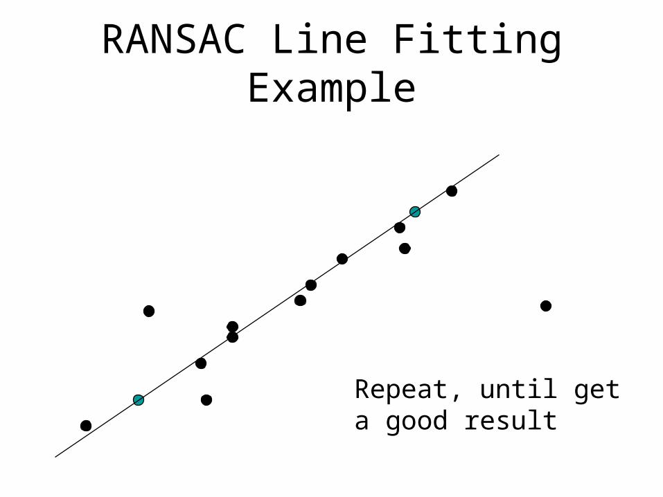
RANSAC Line Fitting Example
Task:
Estimate best line
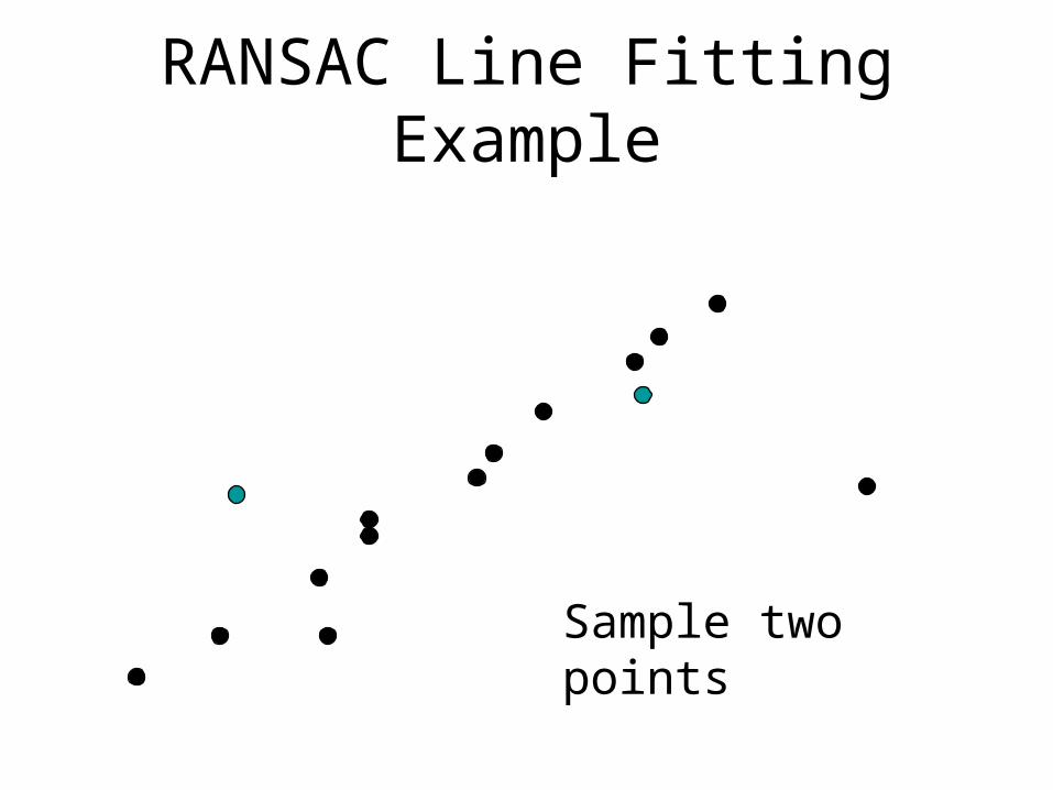
RANSAC Line Fitting Example
Sample two points
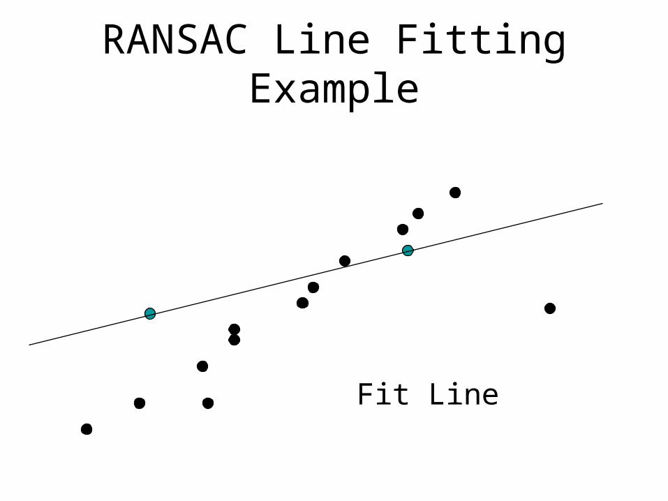
RANSAC Line Fitting Example
Fit Line
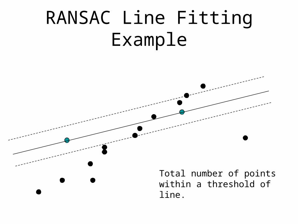
RANSAC Line Fitting Example
Total number of points within a threshold of line.
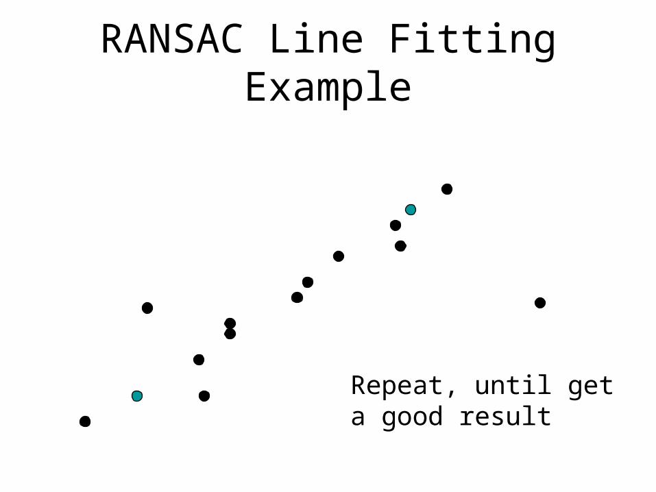
RANSAC Line Fitting Example
Repeat, until get a good result
RANSAC Line Fitting Example
Repeat, until get a good result

RANSAC Line Fitting Example
Repeat, until get a good result

How Many Samples?
Choose N so that, with probability p, at least one random sample is free from outliers. e.g. p=0.99
sepN 11log/1log
peNs 111
proportion of outliers es 5% 10% 20% 25% 30% 40% 50%2 2 3 5 6 7 11 173 3 4 7 9 11 19 354 3 5 9 13 17 34 725 4 6 12 17 26 57 1466 4 7 16 24 37 97 2937 4 8 20 33 54 163 5888 5 9 26 44 78 272 1177
Affine transform

How Many Samples?
Choose N so that, with probability p, at least one random sample is free from outliers. e.g. p=0.99
sepN 11log/1log
peNs 111
proportion of outliers es 5% 10% 20% 25% 30% 40% 50%2 2 3 5 6 7 11 173 3 4 7 9 11 19 354 3 5 9 13 17 34 725 4 6 12 17 26 57 1466 4 7 16 24 37 97 2937 4 8 20 33 54 163 5888 5 9 26 44 78 272 1177
Projective transform
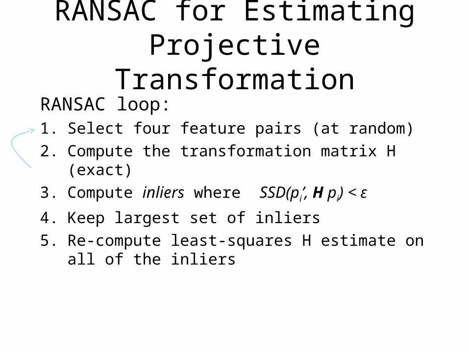
RANSAC for Estimating Projective Transformation
RANSAC loop:1. Select four feature pairs (at random)
2. Compute the transformation matrix H (exact)
3. Compute inliers where SSD(pi’, H pi) < ε
4. Keep largest set of inliers
5. Re-compute least-squares H estimate on all of the inliers
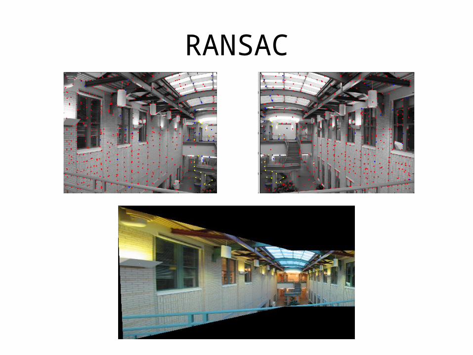
RANSAC
Feature-based Registration
Works for small or large motion
Model the motion within a patch or whole image using a parametric transformation model

Feature-based Registration
Works for small or large motion
Model the motion within a patch or whole image using a parametric transformation model
How to deal with motions that cannot be described by a small number of parameters?
Outline
Image registration
- feature-based approach
- pixel-based approach

Direct (pixel-based) Alignment : Optical flow
Will start by estimating motion of each pixel separatelyThen will consider motion of entire image
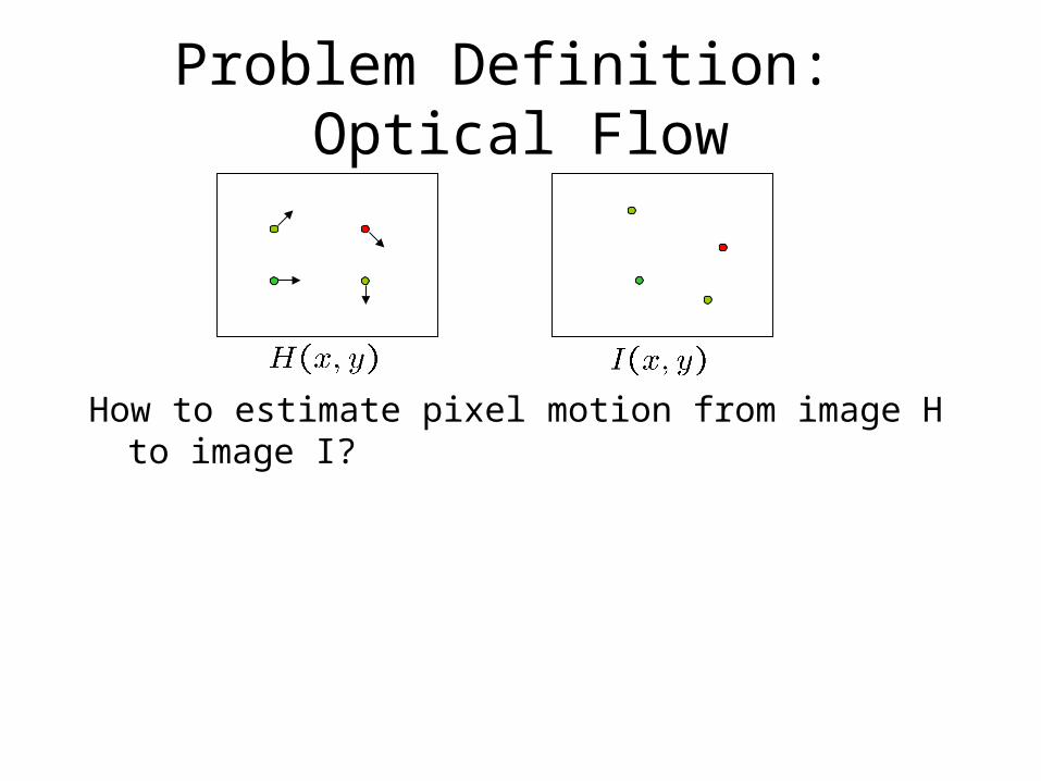
Problem Definition: Optical Flow
How to estimate pixel motion from image H to image I?
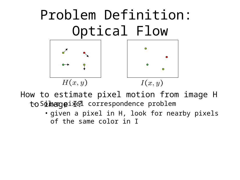
Problem Definition: Optical Flow
How to estimate pixel motion from image H to image I?– Solve pixel correspondence problem
• given a pixel in H, look for nearby pixels of the same color in I
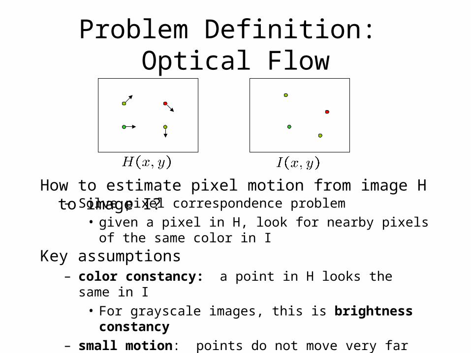
Problem Definition: Optical Flow
How to estimate pixel motion from image H to image I?– Solve pixel correspondence problem
• given a pixel in H, look for nearby pixels of the same color in I
Key assumptions– color constancy: a point in H looks the same in I
• For grayscale images, this is brightness constancy– small motion: points do not move very far
This is called the optical flow problem
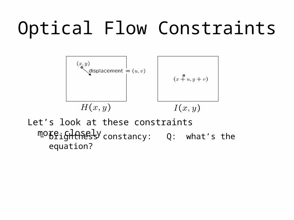
Optical Flow Constraints
Let’s look at these constraints more closely– brightness constancy: Q: what’s the equation?
Optical Flow Constraints
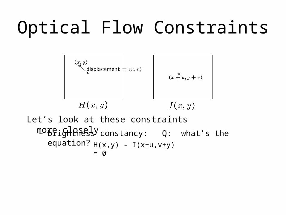
Let’s look at these constraints more closely– brightness constancy: Q: what’s the equation?
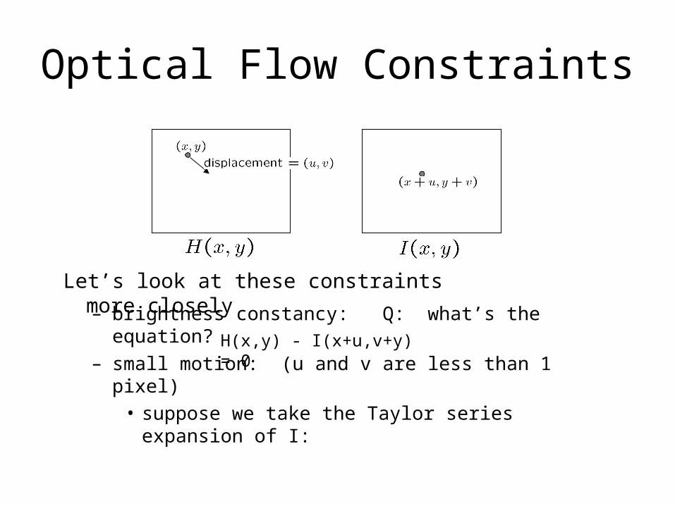
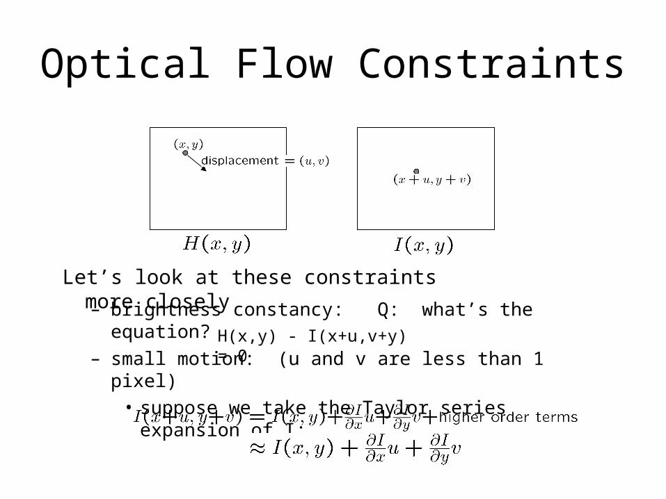
H(x,y) - I(x+u,v+y) = 0
Optical Flow Constraints
Let’s look at these constraints more closely– brightness constancy: Q: what’s the equation?
– small motion: (u and v are less than 1 pixel)• suppose we take the Taylor series expansion of I:
H(x,y) - I(x+u,v+y) = 0
Optical Flow Constraints
Let’s look at these constraints more closely– brightness constancy: Q: what’s the equation?
– small motion: (u and v are less than 1 pixel)• suppose we take the Taylor series expansion of I:
H(x,y) - I(x+u,v+y) = 0
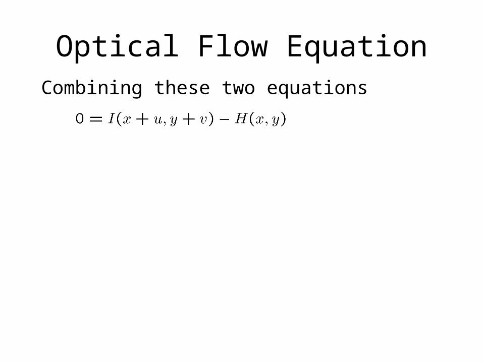
Optical Flow EquationCombining these two equations
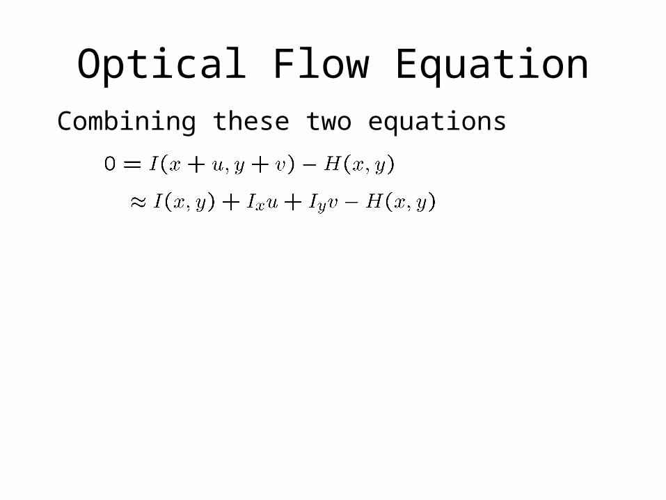
Optical Flow EquationCombining these two equations
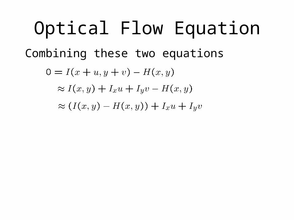
Optical Flow EquationCombining these two equations

Optical Flow EquationCombining these two equations
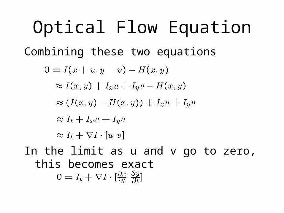
Optical Flow EquationCombining these two equations
In the limit as u and v go to zero, this becomes exact

Optical Flow Equation
How many unknowns and equations per pixel?
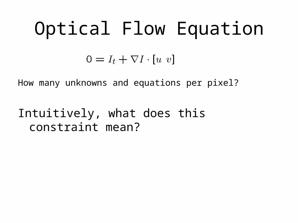
Optical Flow Equation
How many unknowns and equations per pixel?
Intuitively, what does this constraint mean?

Optical Flow Equation
How many unknowns and equations per pixel?
Intuitively, what does this constraint mean?– The component of the flow in the gradient direction is
determined– The component of the flow parallel to an edge is
unknown
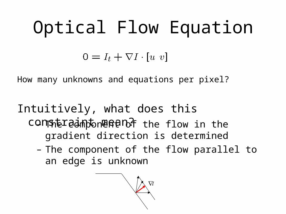
Optical Flow Equation
How many unknowns and equations per pixel?
Intuitively, what does this constraint mean?– The component of the flow in the gradient direction is
determined– The component of the flow parallel to an edge is
unknown
I
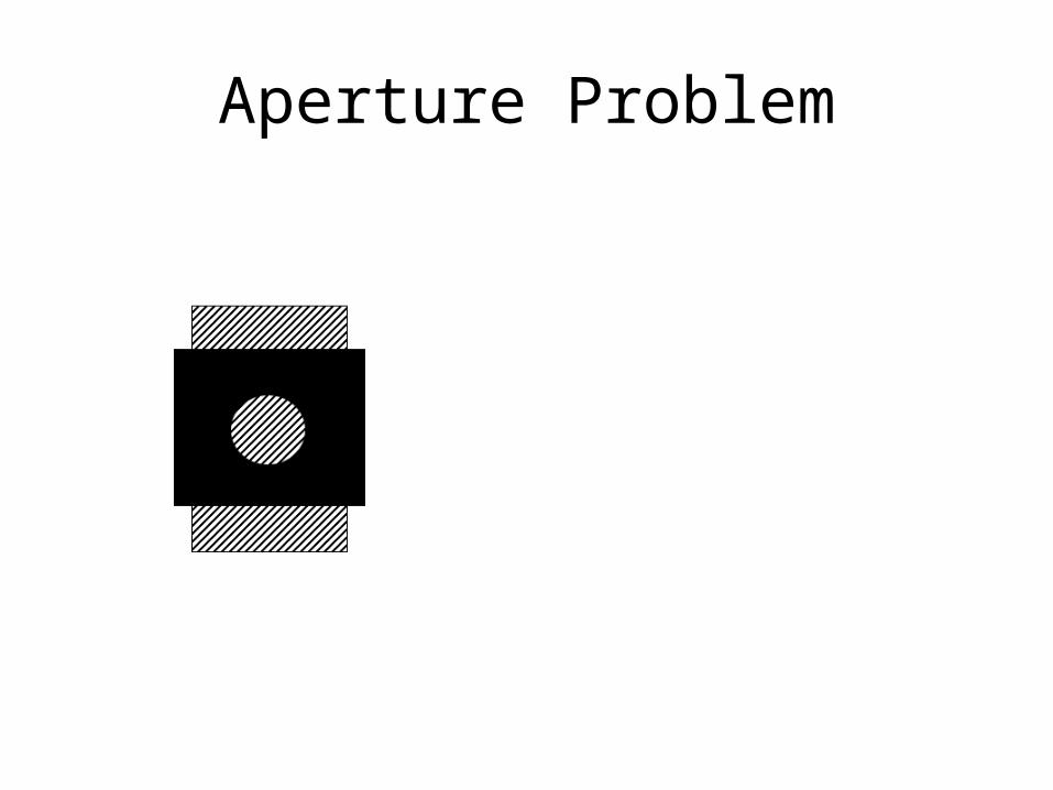
Aperture Problem
Aperture Problem
Stripes moved upwards 6 pixels
Stripes moved left 5 pixels
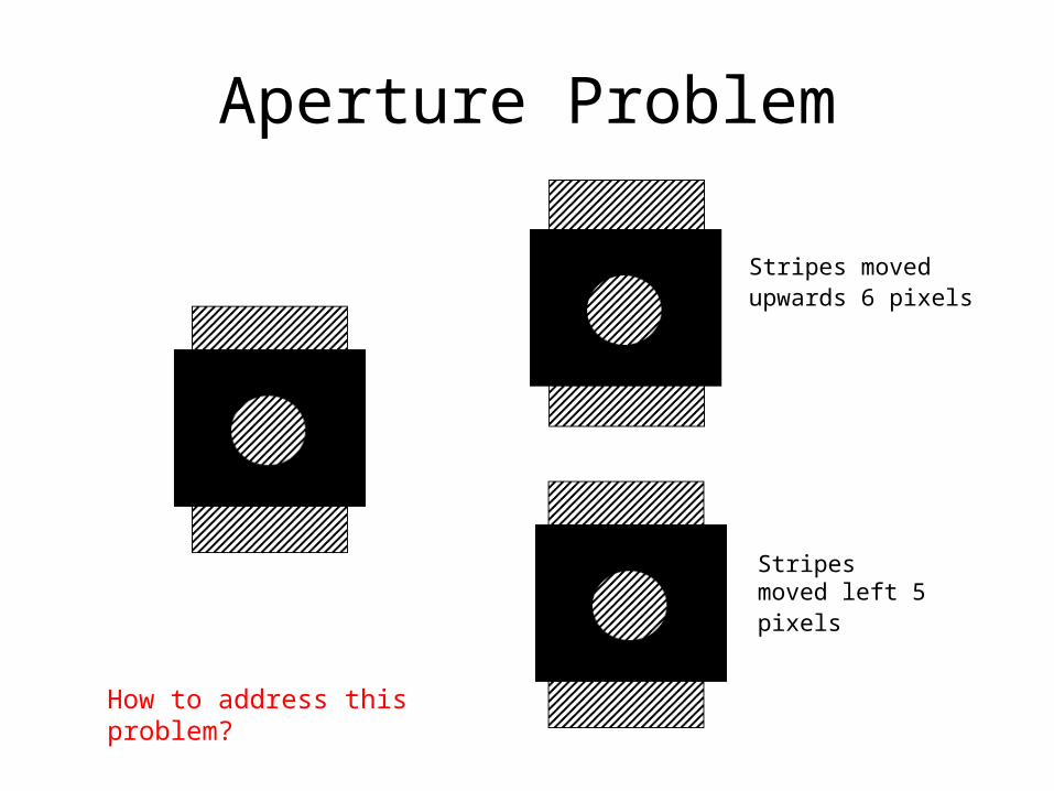
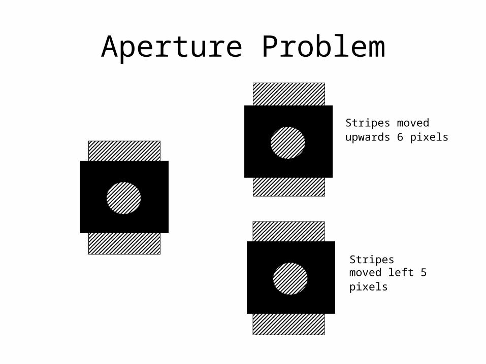
Aperture Problem
Stripes moved upwards 6 pixels
Stripes moved left 5 pixels
How to address this problem?
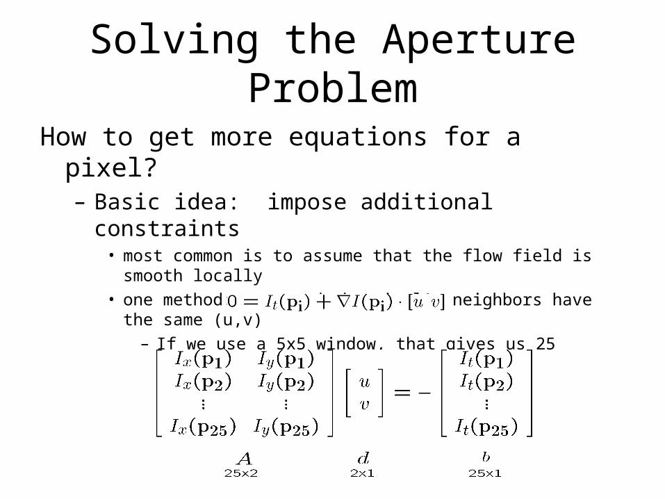
Solving the Aperture Problem
How to get more equations for a pixel?– Basic idea: impose additional constraints
• most common is to assume that the flow field is smooth locally
• one method: pretend the pixel’s neighbors have the same (u,v)
– If we use a 5x5 window, that gives us 25 equations per pixel!
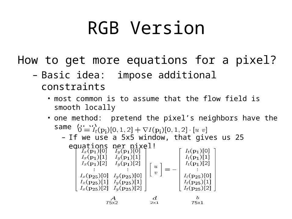
RGB Version
How to get more equations for a pixel?– Basic idea: impose additional constraints
• most common is to assume that the flow field is smooth locally
• one method: pretend the pixel’s neighbors have the same (u,v)
– If we use a 5x5 window, that gives us 25 equations per pixel!
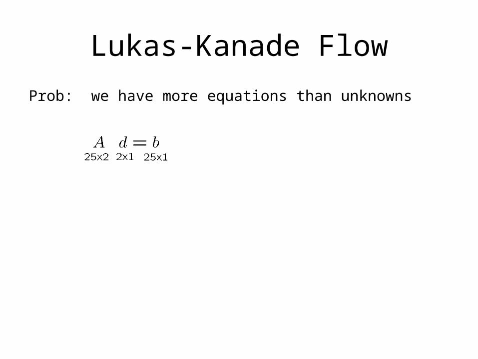
Lukas-Kanade Flow
Prob: we have more equations than unknowns
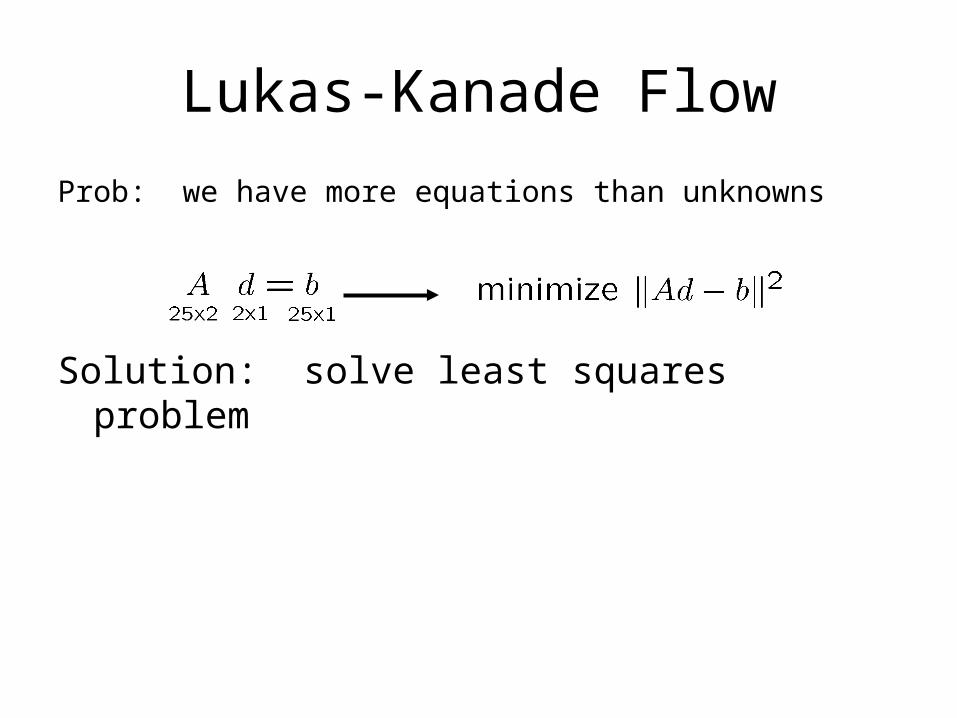
Lukas-Kanade Flow
Prob: we have more equations than unknowns
Solution: solve least squares problem
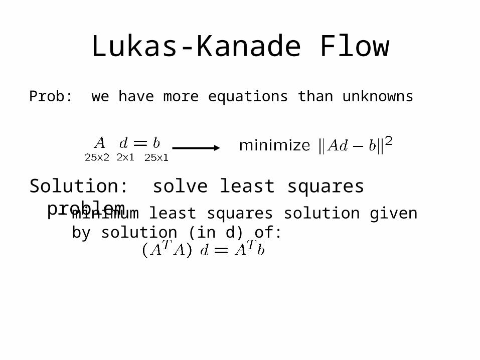
Lukas-Kanade Flow
Prob: we have more equations than unknowns
Solution: solve least squares problem– minimum least squares solution given by solution
(in d) of:

Lukas-Kanade Flow
– The summations are over all pixels in the K x K window
– This technique was first proposed by Lukas & Kanade (1981)
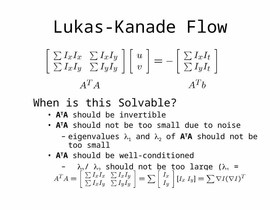
Lukas-Kanade Flow
When is this Solvable?• ATA should be invertible • ATA should not be too small due to noise
– eigenvalues 1 and 2 of ATA should not be too small• ATA should be well-conditioned
– 1/ 2 should not be too large (1 = larger eigenvalue)
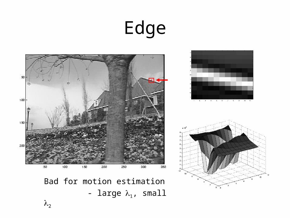
Edge
Bad for motion estimation
- large1, small 2
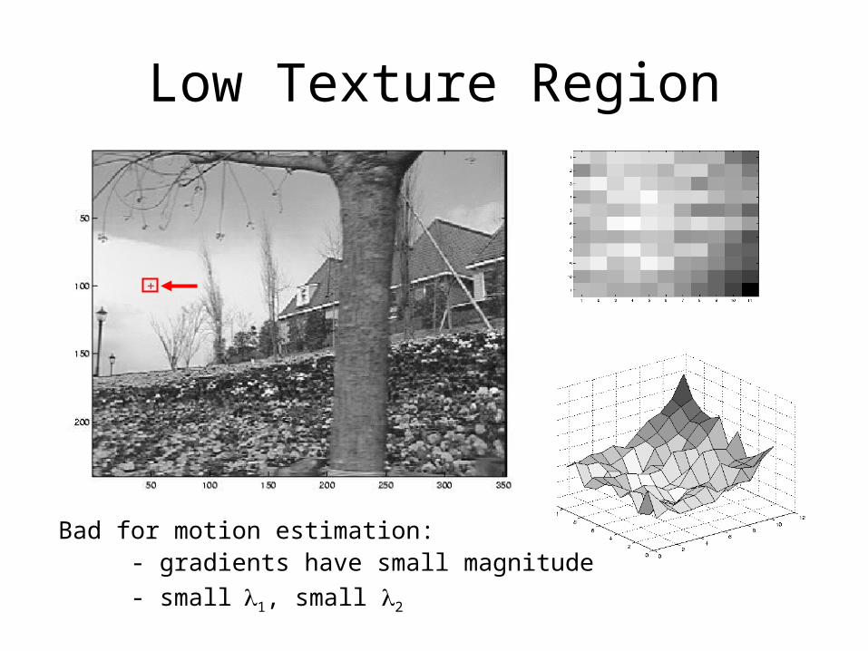
Low Texture Region
Bad for motion estimation: - gradients have small magnitude
- small1, small 2
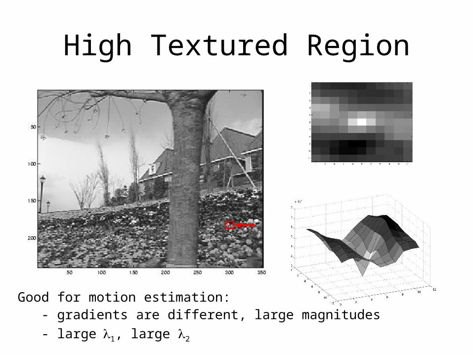
High Textured Region
Good for motion estimation: - gradients are different, large magnitudes
- large1, large 2

Observation
This is a two image problem BUT– Can measure sensitivity by just looking at one of the
images!– This tells us which pixels are easy to track, which are
hard• very useful later on when we do feature tracking...
Errors in Lucas-Kanade
What are the potential causes of errors in this procedure?– Suppose ATA is easily invertible– Suppose there is not much noise in the image
Errors in Lucas-Kanade
What are the potential causes of errors in this procedure?– Suppose ATA is easily invertible– Suppose there is not much noise in the image
When our assumptions are violated– Brightness constancy is not satisfied– The motion is not small– A point does not move like its neighbors
• window size is too large• what is the ideal window size?

Iterative RefinementIterative Lukas-Kanade Algorithm
1. Estimate velocity at each pixel by solving Lucas-Kanade equations
2. Warp H towards I using the estimated flow field- use image warping techniques
3. Repeat until convergence
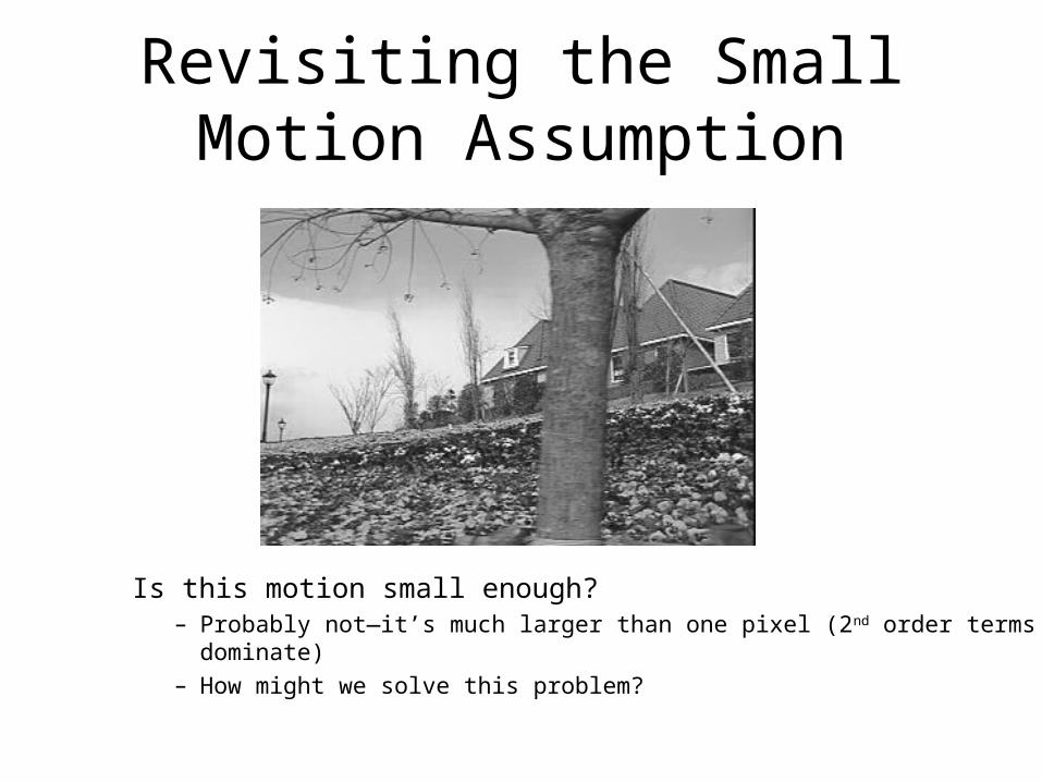
Revisiting the Small Motion Assumption
Is this motion small enough?– Probably not—it’s much larger than one pixel (2nd order terms dominate)– How might we solve this problem?
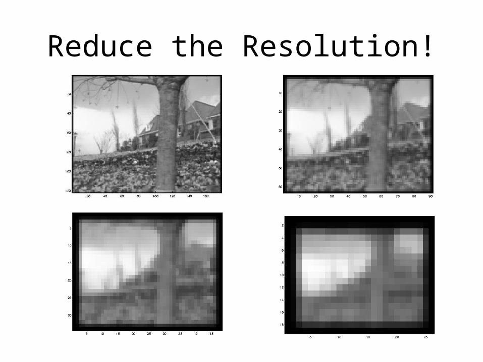
Reduce the Resolution!
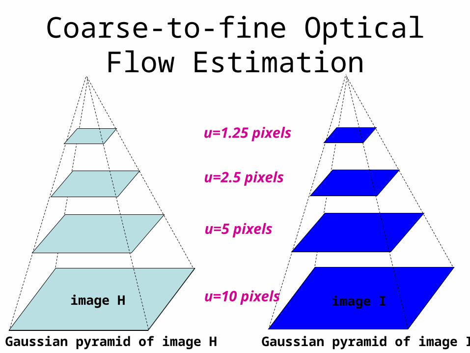
image Iimage H
Gaussian pyramid of image H Gaussian pyramid of image I
image Iimage H u=10 pixels
u=5 pixels
u=2.5 pixels
u=1.25 pixels
Coarse-to-fine Optical Flow Estimation
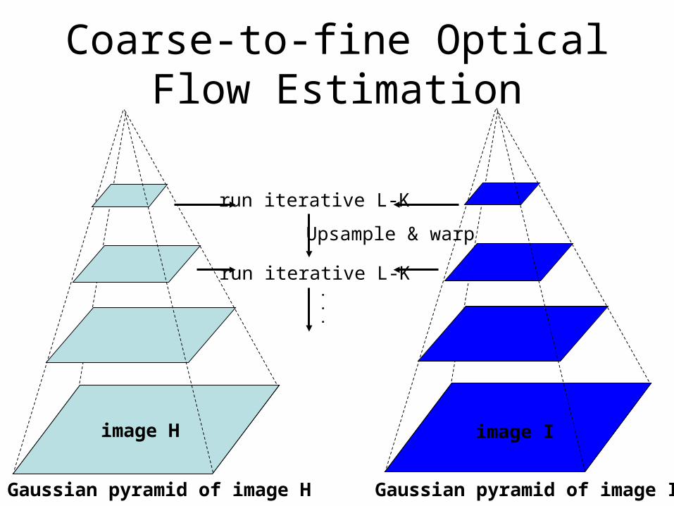
image Iimage J
Gaussian pyramid of image H Gaussian pyramid of image I
image Iimage H
Coarse-to-fine Optical Flow Estimation
run iterative L-K
run iterative L-K
Upsample & warp
.
.
.
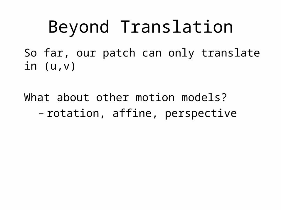
Beyond TranslationSo far, our patch can only translate in (u,v)
What about other motion models?– rotation, affine, perspective
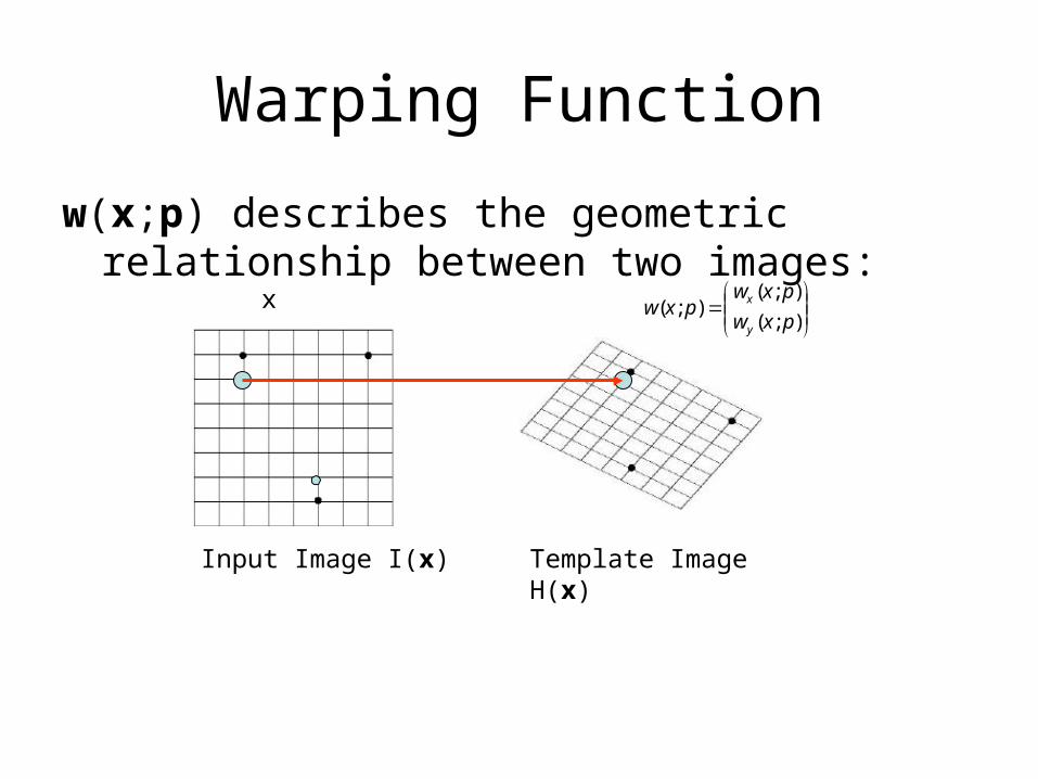
Warping Function
w(x;p) describes the geometric relationship between two images:
);(
);();(
pxw
pxwpxw
y
x
Template Image H(x)Input Image I(x)
x
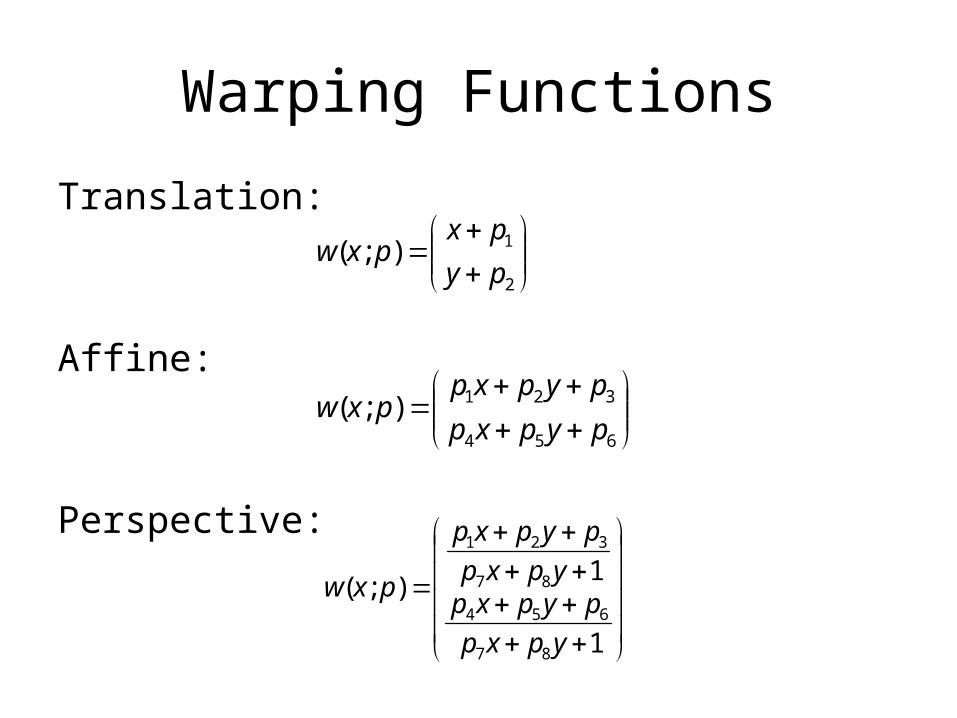
Warping Functions
Translation:
Affine:
Perspective:
2
1);(py
pxpxw
1
1);(
87
654
87
321
ypxp
pypxpypxp
pypxp
pxw
654
321);(pypxp
pypxppxw
Image Registration
Find the warping parameter p that minimizes the intensity difference between template image and the warped input image
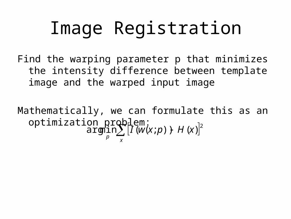
Image Registration
Find the warping parameter p that minimizes the intensity difference between template image and the warped input image
Mathematically, we can formulate this as an optimization problem:
xp
xHpxwI 2)());((minarg
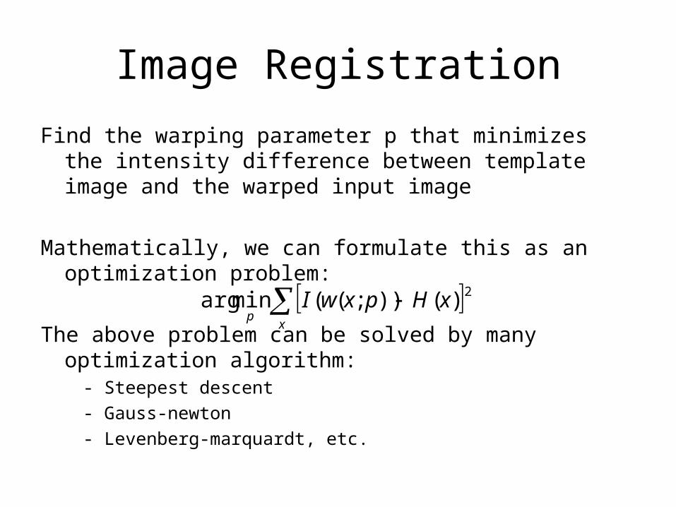
Image Registration
Find the warping parameter p that minimizes the intensity difference between template image and the warped input image
Mathematically, we can formulate this as an optimization problem:
The above problem can be solved by many optimization algorithm:
- Steepest descent
- Gauss-newton
- Levenberg-marquardt, etc.
x
pxHpxwI 2)());((minarg
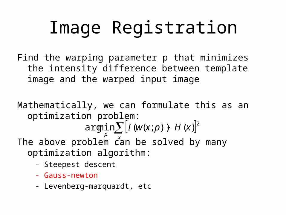
Image Registration
Find the warping parameter p that minimizes the intensity difference between template image and the warped input image
Mathematically, we can formulate this as an optimization problem:
The above problem can be solved by many optimization algorithm:
- Steepest descent
- Gauss-newton
- Levenberg-marquardt, etc
x
pxHpxwI 2)());((minarg
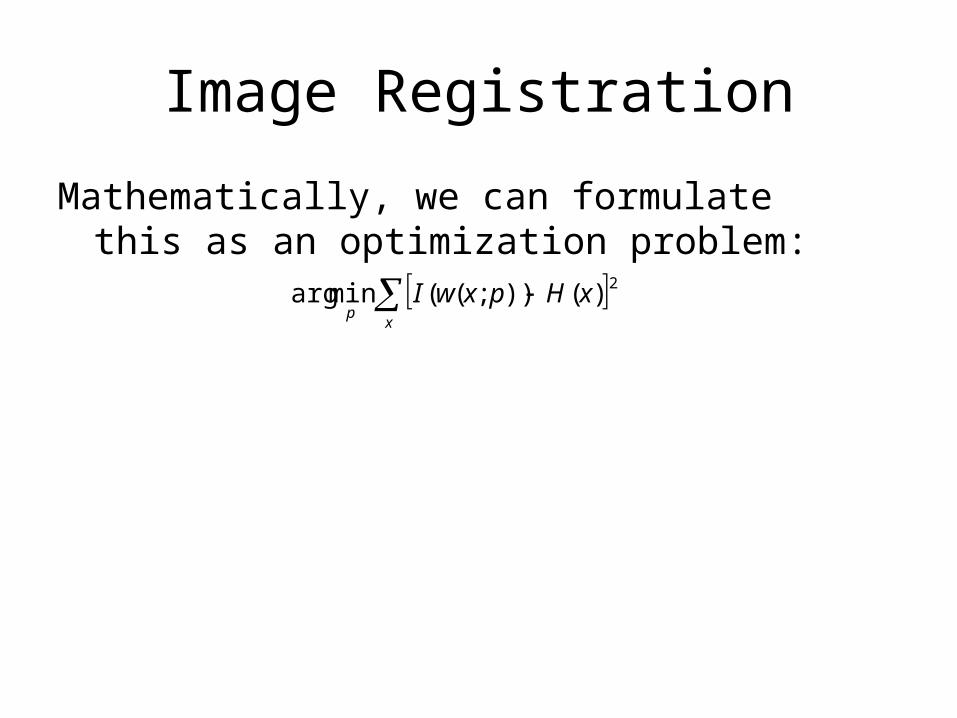
Image Registration
Mathematically, we can formulate this as an optimization problem:
x
pxHpxwI 2)());((minarg
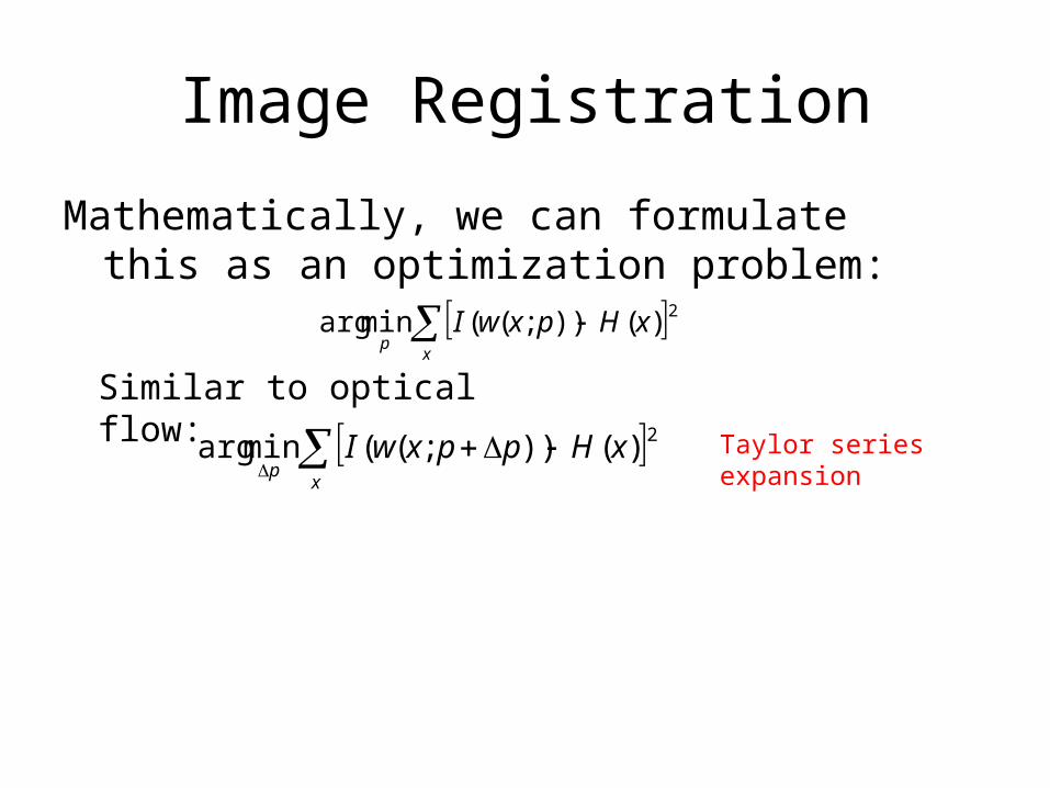
Image Registration
Mathematically, we can formulate this as an optimization problem:
x
pxHpxwI 2)());((minarg
xp
xHppxwI 2)());((minarg Taylor series expansion
Similar to optical flow:
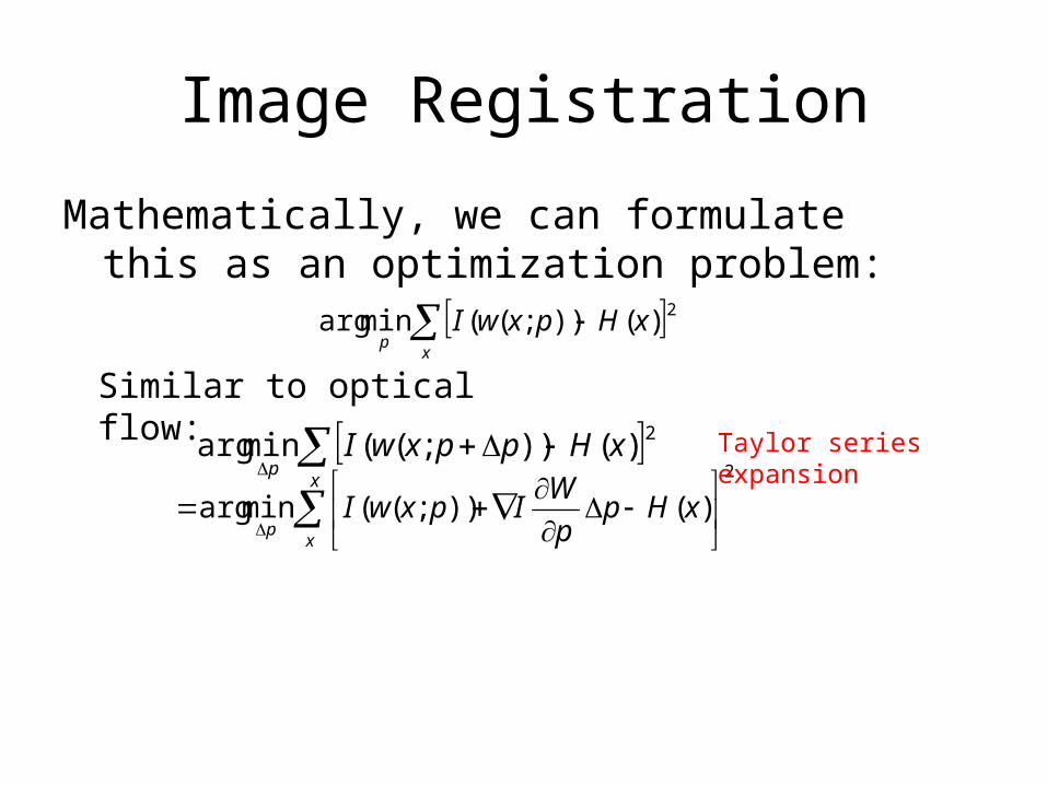
Image Registration
Mathematically, we can formulate this as an optimization problem:
x
pxHpxwI 2)());((minarg
xp
xHppxwI 2)());((minarg
xx
pxHp
p
WIpxwI
2
)());((minarg
Taylor series expansion
Similar to optical flow:
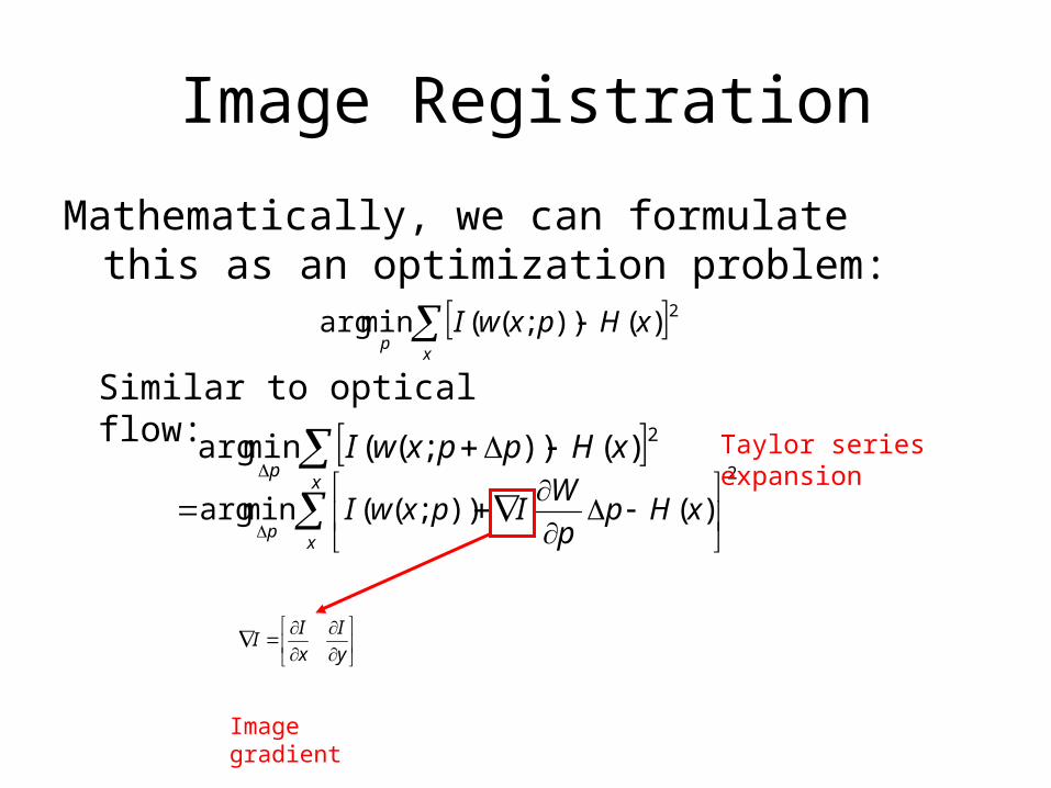
Image Registration
Mathematically, we can formulate this as an optimization problem:
x
pxHpxwI 2)());((minarg
xp
xHppxwI 2)());((minarg
xx
pxHp
p
WIpxwI
2
)());((minarg
y
I
x
II
Taylor series expansion
Image gradient
Similar to optical flow:

Image Registration
Mathematically, we can formulate this as an optimization problem:
xp
xHpxwI 2)());((minarg
xp
xHppxwI 2)());((minarg
xx
pxHp
p
WIpxwI
2
)());((minarg
y
I
x
II
21
1
...
...
p
w
p
wp
w
p
w
p
w
yy
n
xx
10
01
p
w
Taylor series expansion
Image gradient
1000
0001
yx
yx
p
w
translation
affine
……
Similar to optical flow:
Jacobian matrix
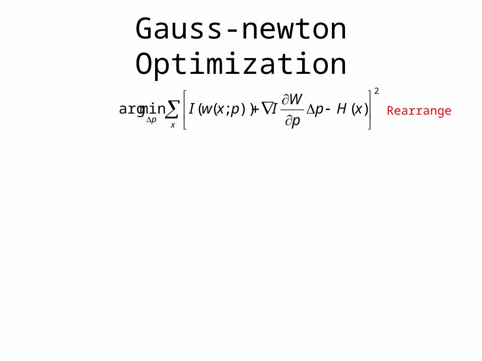
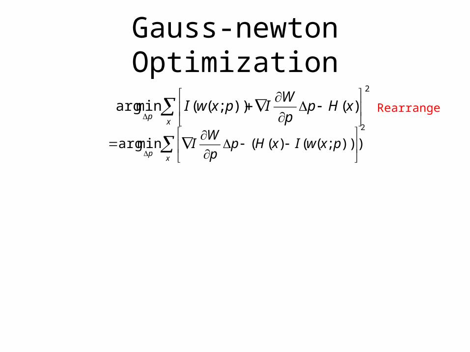
Gauss-newton Optimization
Rearrange
xp
xHpp
WIpxwI
2
)());((minarg
Gauss-newton Optimization
xp
pxwIxHpp
WI
2
)));(()((minarg
Rearrange
xp
xHpp
WIpxwI
2
)());((minarg
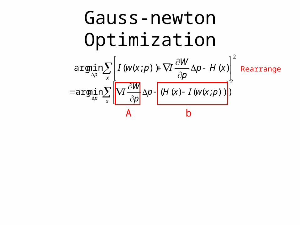
Gauss-newton Optimization
xp
pxwIxHpp
WI
2
)));(()((minarg
Rearrange
A
xp
xHpp
WIpxwI
2
)());((minarg
b
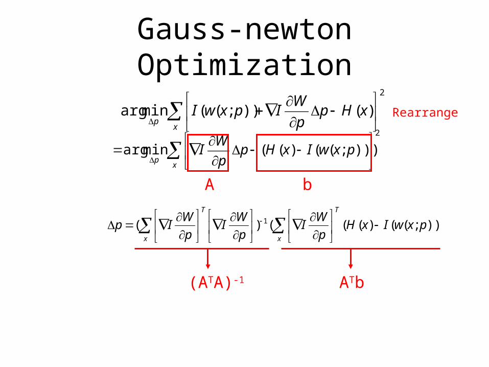
Gauss-newton Optimization
xp
pxwIxHpp
WI
2
)));(()((minarg
)));(()((()( 1 pxwIxHp
WI
p
WI
p
WIp
T
xx
T
Rearrange
A
ATb
xp
xHpp
WIpxwI
2
)());((minarg
b
(ATA)-1
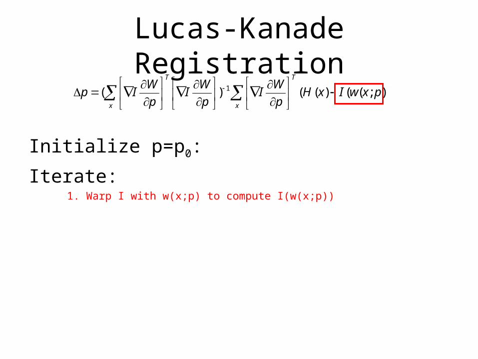
Lucas-Kanade Registration
Initialize p=p0:
Iterate: 1. Warp I with w(x;p) to compute I(w(x;p))
));(()(()( 1 pxwIxHp
WI
p
WI
p
WIp
T
xx
T

Lucas-Kanade Registration
Initialize p=p0:
Iterate: 1. Warp I with w(x;p) to compute I(w(x;p))
2. Compute the error image
));(()(()( 1 pxwIxHp
WI
p
WI
p
WIp
T
xx
T
Lucas-Kanade Registration
Initialize p=p0:
Iterate: 1. Warp I with w(x;p) to compute I(w(x;p))
2. Compute the error image
3. Warp the gradient with w(x;p)
));(()(()( 1 pxwIxHp
WI
p
WI
p
WIp
T
xx
T
I
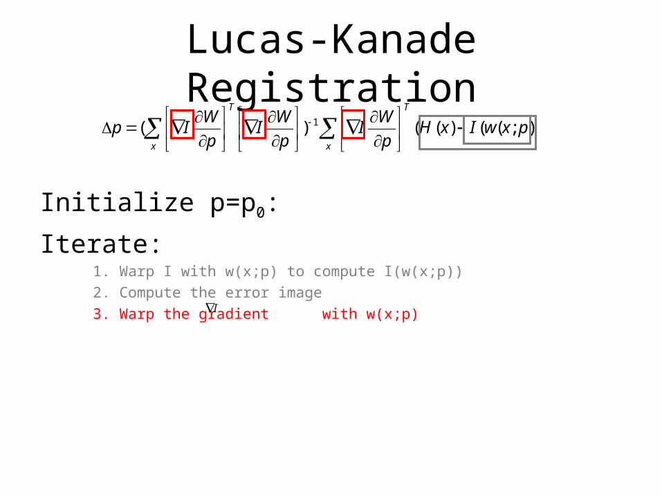
Lucas-Kanade Registration
Initialize p=p0:
Iterate: 1. Warp I with w(x;p) to compute I(w(x;p))
2. Compute the error image
3. Warp the gradient with w(x;p)
4. Evaluate the Jacobian at (x;p)
));(()(()( 1 pxwIxHp
WI
p
WI
p
WIp
T
xx
T
I
p
w
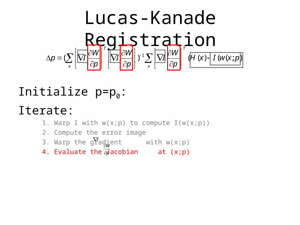
Lucas-Kanade Registration
Initialize p=p0:
Iterate: 1. Warp I with w(x;p) to compute I(w(x;p))
2. Compute the error image
3. Warp the gradient with w(x;p)
4. Evaluate the Jacobian at (x;p)
5. Compute the
));(()(()( 1 pxwIxHp
WI
p
WI
p
WIp
T
xx
T
I
p
w
p
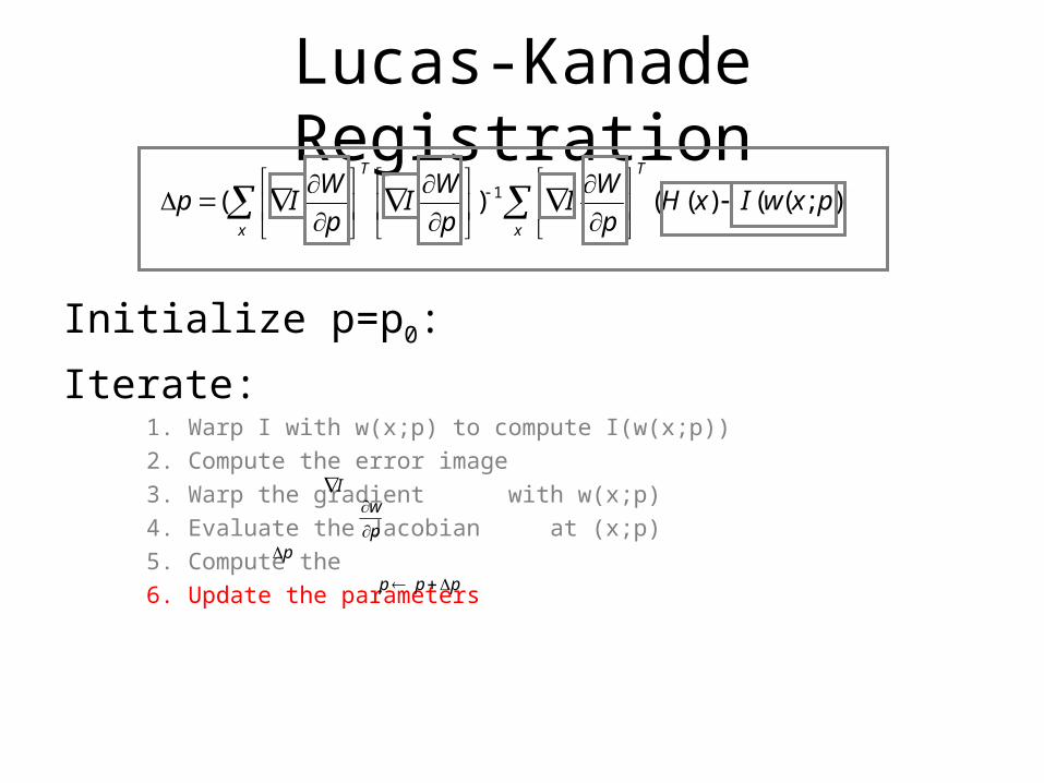
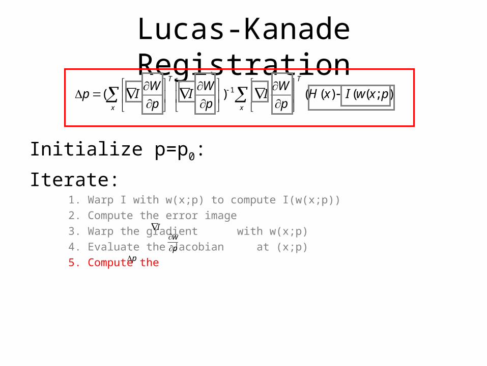
Lucas-Kanade Registration
Initialize p=p0:
Iterate: 1. Warp I with w(x;p) to compute I(w(x;p))
2. Compute the error image
3. Warp the gradient with w(x;p)
4. Evaluate the Jacobian at (x;p)
5. Compute the
6. Update the parameters
));(()(()( 1 pxwIxHp
WI
p
WI
p
WIp
T
xx
T
I
p
w
p
ppp
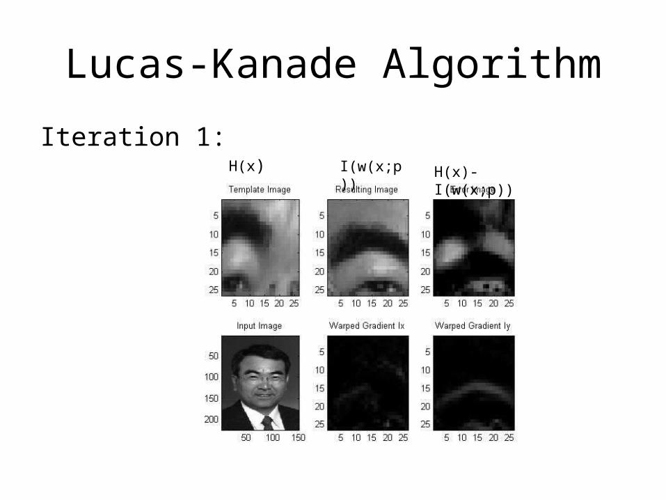
Lucas-Kanade Algorithm
Iteration 1:H(x) I(w(x;p)) H(x)-I(w(x;p))

Lucas-Kanade Algorithm
Iteration 2:H(x) I(w(x;p)) H(x)-I(w(x;p))
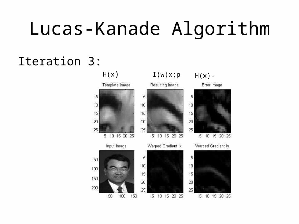
Lucas-Kanade Algorithm
Iteration 3:H(x) I(w(x;p)) H(x)-I(w(x;p))

Lucas-Kanade Algorithm
Iteration 4:H(x) I(w(x;p)) H(x)-I(w(x;p))

Lucas-Kanade Algorithm
Iteration 5:H(x) I(w(x;p)) H(x)-I(w(x;p))

Lucas-Kanade Algorithm
Iteration 6:H(x) I(w(x;p)) H(x)-I(w(x;p))

Lucas-Kanade Algorithm
Iteration 7:H(x) I(w(x;p)) H(x)-I(w(x;p))

Lucas-Kanade Algorithm
Iteration 8:H(x) I(w(x;p)) H(x)-I(w(x;p))

Lucas-Kanade Algorithm
Iteration 9:H(x) I(w(x;p)) H(x)-I(w(x;p))
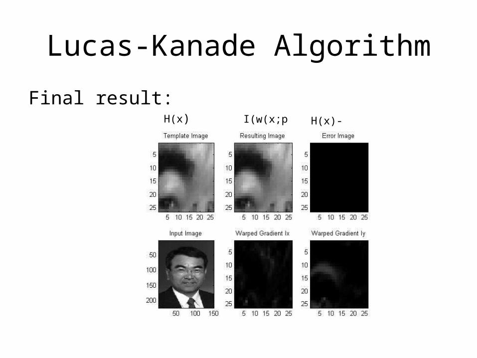
Lucas-Kanade Algorithm
Final result:H(x) I(w(x;p)) H(x)-I(w(x;p))
Lucas-Kanade for Image Alignment
Pros:– All pixels get used in matching– Can get sub-pixel accuracy (important for good
mosaicing!)– Relatively fast and simple
Cons:– Prone to local minima– Relative small movement