Computational Fluid Dynamics Validation of a Single Central Nozzle Supersonic Retropropulsion Configuration

AE8900 MS Special Problems Report Space Systems Design Lab (SSDL)

Guggenheim School of Aerospace Engineering Georgia Institute of Technology

Atlanta, GA

Author: Christopher E. Cordell, Jr.

Advisor: Dr. Robert D. Braun

May 25, 2009

1

Computational Fluid Dynamics Validation of a Single, Central Nozzle Supersonic Retropropulsion Configuration

Christopher E. Cordell, Jr. Georgia Institute of Technology, Atlanta, GA 30332

Dr. Robert D. Braun

Advisor, Georgia Institute of Technology, Atlanta, GA 30332

Supersonic retropropulsion provides an option that can potentially enhance drag characteristics of high mass entry, descent, and landing systems. Preliminary flow field and vehicle aerodynamic characteristics have been found in wind tunnel experiments; however, these only cover specific vehicle configurations and freestream conditions. In order to generate useful aerodynamic data that can be used in a trajectory simulation, a quicker method of determining vehicle aerodynamics is required to model supersonic retropropulsion effects. Using computational fluid dynamics, flow solutions can be determined which yield the desired aerodynamic information. The flow field generated in a supersonic retropropulsion scenario is complex, which increases the difficulty of generating an accurate computational solution. By validating the computational solutions against available wind tunnel data, the confidence in accurately capturing the flow field is increased, and methods to reduce the time required to generate a solution can be determined. Fun3D, a computational fluid dynamics code developed at NASA Langley Research Center, is capable of modeling the flow field structure and vehicle aerodynamics seen in previous wind tunnel experiments. Axial locations of the jet terminal shock, stagnation point, and bow shock show the same trends which were found in the wind tunnel, and the surface pressure distribution and drag coefficient are also consistent with available data. The flow solution is dependent on the computational grid used, where a grid which is too coarse does not resolve all of the flow features correctly. Refining the grid will increase the fidelity of the solution; however, the calculations will take longer if there are more cells in the computational grid.

Nomenclature A = model base area Pexit = nozzle exit pressure Aexit = nozzle exit area P∞ = freestream pressure CD = drag coefficient Pt,jet = nozzle total pressure CP = pressure coefficient q∞ = freestream dynamic pressure CT = thrust coefficient R = specific gas constant γ = ratio of specific heats T = thrust Mexit = nozzle exit Mach number T∞ = freestream temperature ρ = density Tjet = nozzle total temperature ρ∞ = freestream density u = nozzle exit axial velocity component P = pressure V∞ = freestream velocity P0,jet = nozzle total pressure y = nozzle exit radial position component BFI = blunt flow interaction CFD = computational fluid dynamics EDL = entry, descent, and landing LJP = long jet penetration NASA = National Aeronautics and Space Administration SRP = supersonic retropropulsion

2

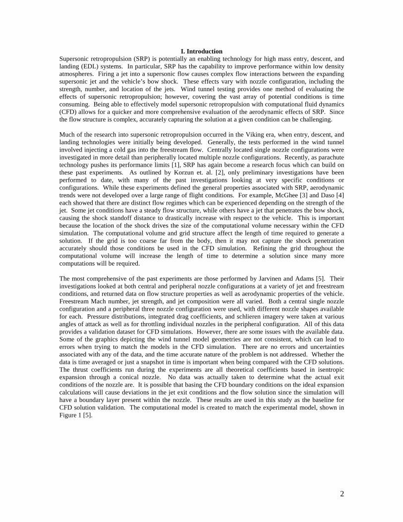
I. Introduction Supersonic retropropulsion (SRP) is potentially an enabling technology for high mass entry, descent, and landing (EDL) systems. In particular, SRP has the capability to improve performance within low density atmospheres. Firing a jet into a supersonic flow causes complex flow interactions between the expanding supersonic jet and the vehicle’s bow shock. These effects vary with nozzle configuration, including the strength, number, and location of the jets. Wind tunnel testing provides one method of evaluating the effects of supersonic retropropulsion; however, covering the vast array of potential conditions is time consuming. Being able to effectively model supersonic retropropulsion with computational fluid dynamics (CFD) allows for a quicker and more comprehensive evaluation of the aerodynamic effects of SRP. Since the flow structure is complex, accurately capturing the solution at a given condition can be challenging. Much of the research into supersonic retropropulsion occurred in the Viking era, when entry, descent, and landing technologies were initially being developed. Generally, the tests performed in the wind tunnel involved injecting a cold gas into the freestream flow. Centrally located single nozzle configurations were investigated in more detail than peripherally located multiple nozzle configurations. Recently, as parachute technology pushes its performance limits [1], SRP has again become a research focus which can build on these past experiments. As outlined by Korzun et. al. [2], only preliminary investigations have been performed to date, with many of the past investigations looking at very specific conditions or configurations. While these experiments defined the general properties associated with SRP, aerodynamic trends were not developed over a large range of flight conditions. For example, McGhee [3] and Daso [4] each showed that there are distinct flow regimes which can be experienced depending on the strength of the jet. Some jet conditions have a steady flow structure, while others have a jet that penetrates the bow shock, causing the shock standoff distance to drastically increase with respect to the vehicle. This is important because the location of the shock drives the size of the computational volume necessary within the CFD simulation. The computational volume and grid structure affect the length of time required to generate a solution. If the grid is too coarse far from the body, then it may not capture the shock penetration accurately should those conditions be used in the CFD simulation. Refining the grid throughout the computational volume will increase the length of time to determine a solution since many more computations will be required. The most comprehensive of the past experiments are those performed by Jarvinen and Adams [5]. Their investigations looked at both central and peripheral nozzle configurations at a variety of jet and freestream conditions, and returned data on flow structure properties as well as aerodynamic properties of the vehicle. Freestream Mach number, jet strength, and jet composition were all varied. Both a central single nozzle configuration and a peripheral three nozzle configuration were used, with different nozzle shapes available for each. Pressure distributions, integrated drag coefficients, and schlieren imagery were taken at various angles of attack as well as for throttling individual nozzles in the peripheral configuration. All of this data provides a validation dataset for CFD simulations. However, there are some issues with the available data. Some of the graphics depicting the wind tunnel model geometries are not consistent, which can lead to errors when trying to match the models in the CFD simulation. There are no errors and uncertainties associated with any of the data, and the time accurate nature of the problem is not addressed. Whether the data is time averaged or just a snapshot in time is important when being compared with the CFD solutions. The thrust coefficients run during the experiments are all theoretical coefficients based in isentropic expansion through a conical nozzle. No data was actually taken to determine what the actual exit conditions of the nozzle are. It is possible that basing the CFD boundary conditions on the ideal expansion calculations will cause deviations in the jet exit conditions and the flow solution since the simulation will have a boundary layer present within the nozzle. These results are used in this study as the baseline for CFD solution validation. The computational model is created to match the experimental model, shown in Figure 1 [5].

3

Figure 1: Physical Model for Wind Tunnel Experiments [5].

II. Computational Grid Methodology

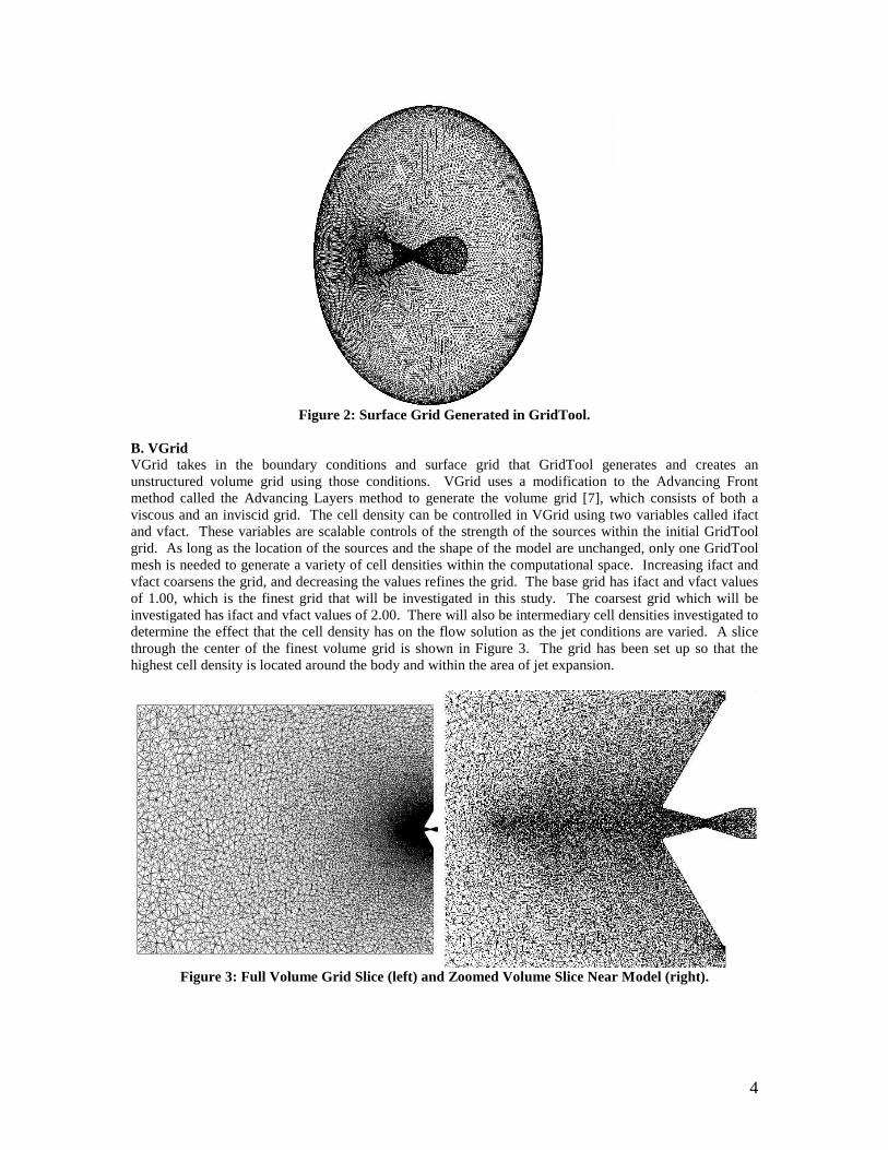
In order to accurately simulate supersonic retropropulsion, the computational grid must be capable of handling the complex flow features which are expected to exist within the flow solution. If the grid is too coarse in some areas, then shocks that exist in those regions will not resolve properly, and some flow features can potentially be lost or misplaced in the flow. The computational grid used for this study has been generated using GridTool and VGrid, which generate boundary surfaces and the volume grid respectively. For this study, the 3-dimensional computational model is based on the experimental model shown in Figure 1. The model is built using units of millimeters, which will be preserved in the grid generation and affect some of the input values for the flow solver, such as the Reynolds number. Since the central nozzle configuration has the most data available, it makes a good baseline for determining the grid resolution required to accurately model the flow field properties. A. GridTool GridTool [6] reads in the geometry .igs file and allows the user to define each surface on the body using patches. The patches define the outward normal for each surface as well as allowing for boundary conditions to be individually applied to each surface. These boundary conditions include the parameters for the jet flow on the patch representing the flow-through boundary inside the nozzle. GridTool also applies the computational farfield boundary for the grid. For supersonic retropropulsion, this is an important factor since some of the jet conditions have the potential to blow the shock far off the body. For this preliminary study, it is not initially known if these scenarios will exist computationally, so the farfield box has been extended to eight times the base diameter of the vehicle in the axial direction, which should contain any shocks that are blown off the body. Studies show that the shock can be blown anywhere from three to six body diameters away from the body and that the flow in these regimes is highly unstable [3], [4], [5]. The exit plane is placed at the shoulder of the vehicle, since the main interest for this study are the aerodynamic effects on the vehicle forebody. This does require that the exit plane boundary condition allow for extrapolation from the inner flow, since there is not enough volume for the flow to fully expand back to freestream conditions. The last important grid feature that GridTool provides is the grid source points and their strengths. The strength of the sources determines the density of the cells in the region around the source. In addition to the sources that get applied to each surface of the body and the edges of the farfield, there is a source line placed along the axis leaving the nozzle. This source provides greater cell density in the region where the jet flow will be expanding and interacting with the bow shock in front of the vehicle. The initial surface grid, which is the finest grid that will be used in the flow solution studies, and the 3-dimensional geometry are shown in Figure 2.

4

Figure 2: Surface Grid Generated in GridTool.

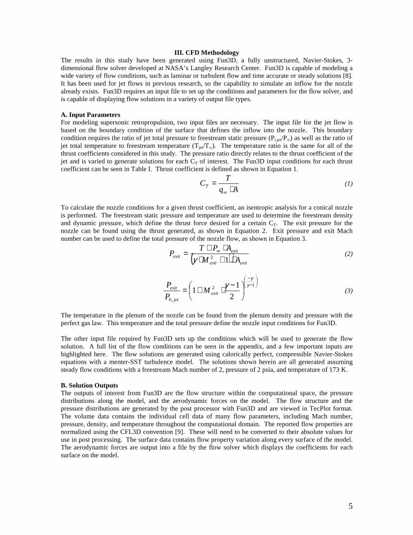
B. VGrid VGrid takes in the boundary conditions and surface grid that GridTool generates and creates an unstructured volume grid using those conditions. VGrid uses a modification to the Advancing Front method called the Advancing Layers method to generate the volume grid [7], which consists of both a viscous and an inviscid grid. The cell density can be controlled in VGrid using two variables called ifact and vfact. These variables are scalable controls of the strength of the sources within the initial GridTool grid. As long as the location of the sources and the shape of the model are unchanged, only one GridTool mesh is needed to generate a variety of cell densities within the computational space. Increasing ifact and vfact coarsens the grid, and decreasing the values refines the grid. The base grid has ifact and vfact values of 1.00, which is the finest grid that will be investigated in this study. The coarsest grid which will be investigated has ifact and vfact values of 2.00. There will also be intermediary cell densities investigated to determine the effect that the cell density has on the flow solution as the jet conditions are varied. A slice through the center of the finest volume grid is shown in Figure 3. The grid has been set up so that the highest cell density is located around the body and within the area of jet expansion.

Figure 3: Full Volume Grid Slice (left) and Zoomed Volume Slice Near Model (right).

5

III. CFD Methodology The results in this study have been generated using Fun3D, a fully unstructured, Navier-Stokes, 3-dimensional flow solver developed at NASA’s Langley Research Center. Fun3D is capable of modeling a wide variety of flow conditions, such as laminar or turbulent flow and time accurate or steady solutions [8]. It has been used for jet flows in previous research, so the capability to simulate an inflow for the nozzle already exists. Fun3D requires an input file to set up the conditions and parameters for the flow solver, and is capable of displaying flow solutions in a variety of output file types. A. Input Parameters For modeling supersonic retropropulsion, two input files are necessary. The input file for the jet flow is based on the boundary condition of the surface that defines the inflow into the nozzle. This boundary condition requires the ratio of jet total pressure to freestream static pressure (Pt,jet/P∞) as well as the ratio of jet total temperature to freestream temperature (Tjet/T∞). The temperature ratio is the same for all of the thrust coefficients considered in this study. The pressure ratio directly relates to the thrust coefficient of the jet and is varied to generate solutions for each CT of interest. The Fun3D input conditions for each thrust coefficient can be seen in Table I. Thrust coefficient is defined as shown in Equation 1.

Aq

TCT ⋅

=∞

(1)

To calculate the nozzle conditions for a given thrust coefficient, an isentropic analysis for a conical nozzle is performed. The freestream static pressure and temperature are used to determine the freestream density and dynamic pressure, which define the thrust force desired for a certain CT. The exit pressure for the nozzle can be found using the thrust generated, as shown in Equation 2. Exit pressure and exit Mach number can be used to define the total pressure of the nozzle flow, as shown in Equation 3.

( ) exitexit

exitexit AM

APTP

⋅+⋅⋅+

= ∞

12γ (2)

−−

−⋅+=12

,0 2

11

γγ

γexit

jet

exit MP

P (3)

The temperature in the plenum of the nozzle can be found from the plenum density and pressure with the perfect gas law. This temperature and the total pressure define the nozzle input conditions for Fun3D. The other input file required by Fun3D sets up the conditions which will be used to generate the flow solution. A full list of the flow conditions can be seen in the appendix, and a few important inputs are highlighted here. The flow solutions are generated using calorically perfect, compressible Navier-Stokes equations with a menter-SST turbulence model. The solutions shown herein are all generated assuming steady flow conditions with a freestream Mach number of 2, pressure of 2 psia, and temperature of 173 K. B. Solution Outputs The outputs of interest from Fun3D are the flow structure within the computational space, the pressure distributions along the model, and the aerodynamic forces on the model. The flow structure and the pressure distributions are generated by the post processor with Fun3D and are viewed in TecPlot format. The volume data contains the individual cell data of many flow parameters, including Mach number, pressure, density, and temperature throughout the computational domain. The reported flow properties are normalized using the CFL3D convention [9]. These will need to be converted to their absolute values for use in post processing. The surface data contains flow property variation along every surface of the model. The aerodynamic forces are output into a file by the flow solver which displays the coefficients for each surface on the model.

6

IV. CFD Solution Validation In order to determine the validity of the Fun3D flow solution for a given jet CT, the output flow solutions are examined and the properties of interest are found. For comparing the flow structure, slices are created in the volume solution, which make the locations of flow features such as the bow shock and jet plume visible. The axial locations of these features are one set of experimental data which is available for comparison with the flow solution. The other major flow property which can be determined from the volume solution is the thrust coefficient of the nozzle. The flow parameters at the nozzle exit can be extracted, which allows for the integration of the thrust coefficient which is being modeled in the flow. This value can be compared to the CT which was used to generate the pressure and temperature ratios initially input into the flow solver. For calculating CT, the velocity and density profiles are extracted in the Z = 0 plane of the flow solution for both the positive and negative values of y, representing the radius from the centerline. The differential thrust coefficient as a function of the radius of the nozzle exit within the planar slice taken from the computational volume is shown in Equation 4, where ρ/ρ∞, u, y, and P/P∞ are Fun3D flow values and ρ∞, P∞, T∞, and A are known from freestream conditions and model geometry.

( )Aq

yP

PPTRu

dCT ⋅

⋅⋅

−+⋅⋅⋅⋅

⋅

=∞

∞∞∞

∞∞ πγ

ρρρ 1

2

(4)

The pressure distributions for the Fun3D solution are calculated from the surface solution file. The normalized output pressures can be converted to pressure coefficients as a function of radial location along the forebody and compared with the available experimental data if applicable. The pressure coefficient at a given radius can be calculated from the surface solution at that point by Equation 5.

∞

∞∞

−

=q

P

PP

CP

1

(5)

To compare aerodynamic forces, only the coefficients along the model forebody are of interest. These are added and compared with available data to ensure that aerodynamic drag is consistent with the wind tunnel data. Reference area is a Fun3D input, so no conversion is necessary when adding the CD for each surface. A. Coarse Grid Trend Comparison Using the coarsest grid, with ifact and vfact values of 2.00, a range of jet thrust conditions have been run and compared with the available wind tunnel data. Table I shows which jet conditions have data available for comparison and the input conditions to define the jet flow within Fun3D. Each of the thrust coefficients listed have been run on the coarsest grid. The CT values which do not have corresponding wind tunnel data have been run to help fill in the trend curves and ensure that the trends are continuous. The cases are concentrated more in the lower CT values (0.5 – 2.0) because these are the areas where flow properties change more according to the experimental data, and these conditions are more likely to be used in flight. In addition to the conditions with the jet turned on, a baseline solution with an inviscid wall instead of a flow through boundary condition at the nozzle inlet has been run to generate a jet off solution.

Table I: Fun3D Input Conditions and Availability of Experimental Data for Comparison Purposes. Fun3D Inputs Available Experimental Data

CT Pt,jet/P∞ Tjet/T∞ CD CP Distribution Flow Structure 0.47 712.41 1.69 Yes Yes No 0.75 1131.85 1.69 Yes No No 1.05 1581.24 1.69 Yes Yes Yes 1.5 2255.34 1.69 No No No 2 3004.33 1.69 Yes Yes Yes

4.04 6060.21 1.69 Yes Yes Yes 5.5 8247.27 1.69 No No No 7 10494.25 1.69 Yes Yes Yes

7

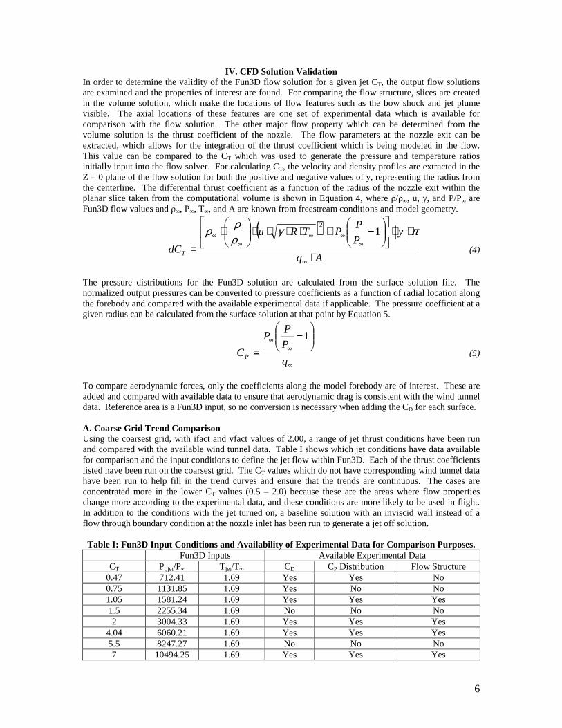
For each thrust coefficient, the solution has been run until it converges. Since SRP consists of complex flow interactions, the flow residuals are not necessarily the only indicator of solution convergence. In addition to monitoring the residuals to check that they are decreasing as the solution evolves, the actual flow properties are also monitored. A solution is considered converged for these cases when the flow structure has settled down and is not noticeably changing by increased iterations. Also, the drag coefficient, pressure distributions, and calculated thrust coefficient are checked to ensure that they have stabilized. When these values settle, this is considered to be converged and the final solution data is taken. The thrust coefficient values for each computational solution are in agreement with the expected values that have been used to calculate the jet conditions for the Fun3D boundary condition. This trend is shown in Figure 4, where the total computational CT reported is integrated over the nozzle exit properties in the volume solution file. Ideally, the points would all fall on the line where the calculated CT is equivalent to the initial input value. For low thrust coefficients, this is mainly the case. At higher thrust coefficients, the divergence between the expected value and the integrated value of CT increases, which is possibly related to the cell density in the region outside of the nozzle. The expected input value of thrust coefficient is also based on ideal expansion through a conical nozzle. The computational solution will model losses in the nozzle, which cause the calculated thrust coefficient to be lower in the Fun3D simulation.

Figure 4: Thrust Coefficient Trend for ifact = 2.00.

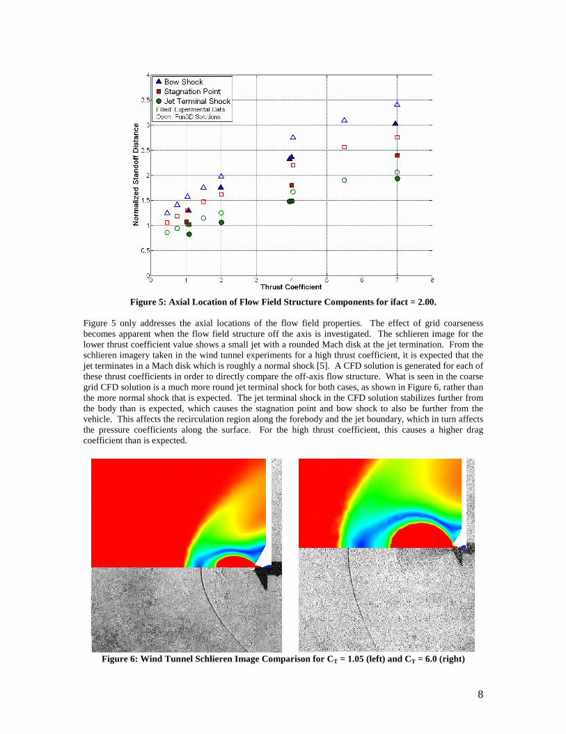
The axial standoff distances of the jet terminal shock, stagnation point, and bow shock are shown in Figure 5. The general trends for the locations of these structures are consistent with what is seen in the experimental data; however the magnitudes of the locations are different from what is expected. There are two main reasons why this may occur. This could be a function of the coarseness of the grid, where the cells are too large to accurately determine where these flow structures should be located along the axis of the body. It also could be related to the periodic motion associated with supersonic retropropulsion. If the wind tunnel data is only taken at a snapshot in time, then it is possible that the dynamic nature of the flow field will not match up with the steady state solution depending on when the image is taken with regards to the motion of the flow field. A more accurate assessment of the validity of the Fun3D steady solution would be to see error bars from the wind tunnel data showing the range of possible locations for each shock component as they move in time, which is not available in the current data set. This also supports that a time accurate solution to the supersonic retropropulsion problem may be required to gain a better understanding of the effects of the jet on the flow field structure.

8

Figure 5: Axial Location of Flow Field Structure Components for ifact = 2.00.

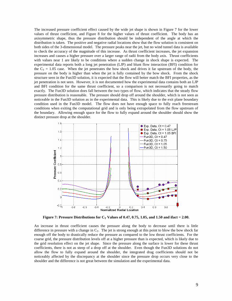
Figure 5 only addresses the axial locations of the flow field properties. The effect of grid coarseness becomes apparent when the flow field structure off the axis is investigated. The schlieren image for the lower thrust coefficient value shows a small jet with a rounded Mach disk at the jet termination. From the schlieren imagery taken in the wind tunnel experiments for a high thrust coefficient, it is expected that the jet terminates in a Mach disk which is roughly a normal shock [5]. A CFD solution is generated for each of these thrust coefficients in order to directly compare the off-axis flow structure. What is seen in the coarse grid CFD solution is a much more round jet terminal shock for both cases, as shown in Figure 6, rather than the more normal shock that is expected. The jet terminal shock in the CFD solution stabilizes further from the body than is expected, which causes the stagnation point and bow shock to also be further from the vehicle. This affects the recirculation region along the forebody and the jet boundary, which in turn affects the pressure coefficients along the surface. For the high thrust coefficient, this causes a higher drag coefficient than is expected.

Figure 6: Wind Tunnel Schlieren Image Comparison for CT = 1.05 (left) and CT = 6.0 (right)

9

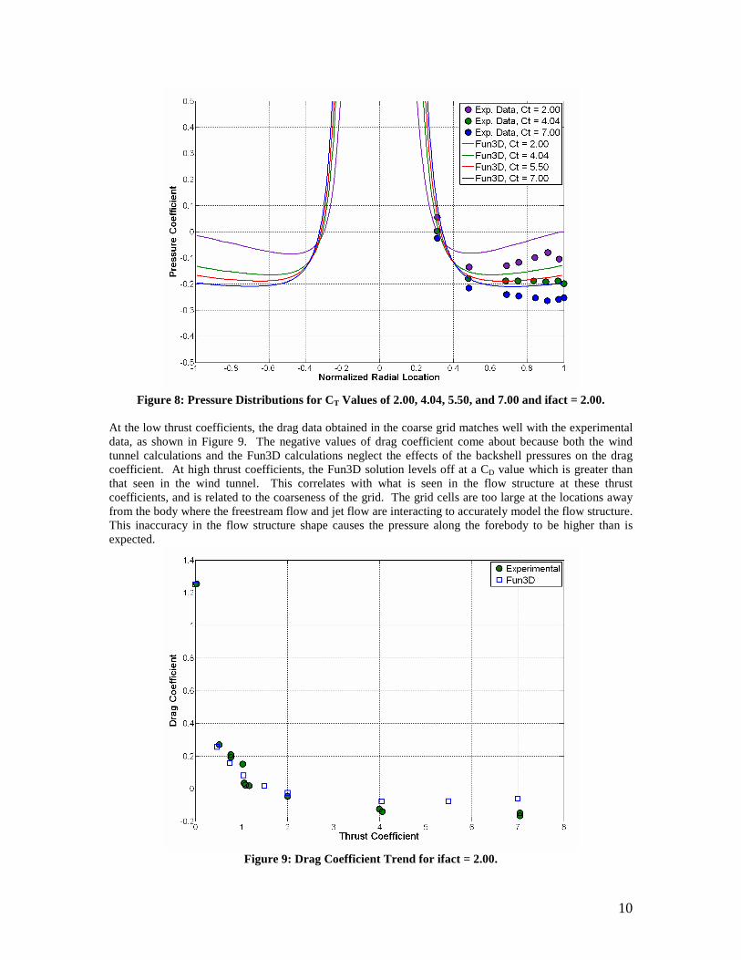
The increased pressure coefficient effect caused by the wide jet shape is shown in Figure 7 for the lower values of thrust coefficient, and Figure 8 for the higher values of thrust coefficient. The body has an axisymmetric shape, thus the pressure distribution should be independent of the angle at which the distribution is taken. The positive and negative radial locations show that the flow solution is consistent on both sides of the 3-dimensional model. The pressure peaks near the jet, but no wind tunnel data is available to check the accuracy of the magnitude of this increase. As thrust coefficient increases, the jet expansion increases and causes a higher pressure over a larger range of radii from the body axis. Thrust coefficients with values near 1 are likely to be conditions where a sudden change in shock shape is expected. The experimental data reports both a long jet penetration (LJP) and blunt flow interaction (BFI) condition for the CT = 1.05 case. When the jet penetrates the bow shock and drives it far upstream of the body, the pressure on the body is higher than when the jet is fully contained by the bow shock. From the shock structure seen in the Fun3D solution, it is expected that the flow will better match the BFI properties, as the jet penetration is not seen. However, it is not documented how the experimental data contains both an LJP and BFI condition for the same thrust coefficient, so a comparison is not necessarily going to match exactly. The Fun3D solution does fall between the two types of flow, which indicates that the steady flow pressure distribution is reasonable. The pressure should drop off around the shoulder, which is not seen as noticeable in the Fun3D solution as in the experimental data. This is likely due to the exit plane boundary condition used in the Fun3D model. The flow does not have enough space to fully reach freestream conditions when exiting the computational grid and is only being extrapolated from the flow upstream of the boundary. Allowing enough space for the flow to fully expand around the shoulder should show the distinct pressure drop at the shoulder.

Figure 7: Pressure Distributions for CT Values of 0.47, 0.75, 1.05, and 1.50 and ifact = 2.00.

An increase in thrust coefficient causes the pressure along the body to decrease until there is little difference in pressure with a change in CT. The jet is strong enough at this point to blow the bow shock far enough off the body to drastically reduce the pressure as compared to the low thrust coefficients. For the coarse grid, the pressure distribution levels off at a higher pressure than is expected, which is likely due to the grid resolution effect on the jet shape. Since the pressure along the surface is lower for these thrust coefficients, there is not as steep of a drop off at the shoulder. Even though the Fun3D solutions do not allow the flow to fully expand around the shoulder, the integrated drag coefficients should not be noticeably affected by the discrepancy at the shoulder since the pressure drop occurs very close to the shoulder and the difference is not great between the simulation and the experimental data.

10

Figure 8: Pressure Distributions for CT Values of 2.00, 4.04, 5.50, and 7.00 and ifact = 2.00.

At the low thrust coefficients, the drag data obtained in the coarse grid matches well with the experimental data, as shown in Figure 9. The negative values of drag coefficient come about because both the wind tunnel calculations and the Fun3D calculations neglect the effects of the backshell pressures on the drag coefficient. At high thrust coefficients, the Fun3D solution levels off at a CD value which is greater than that seen in the wind tunnel. This correlates with what is seen in the flow structure at these thrust coefficients, and is related to the coarseness of the grid. The grid cells are too large at the locations away from the body where the freestream flow and jet flow are interacting to accurately model the flow structure. This inaccuracy in the flow structure shape causes the pressure along the forebody to be higher than is expected.

Figure 9: Drag Coefficient Trend for ifact = 2.00.

11

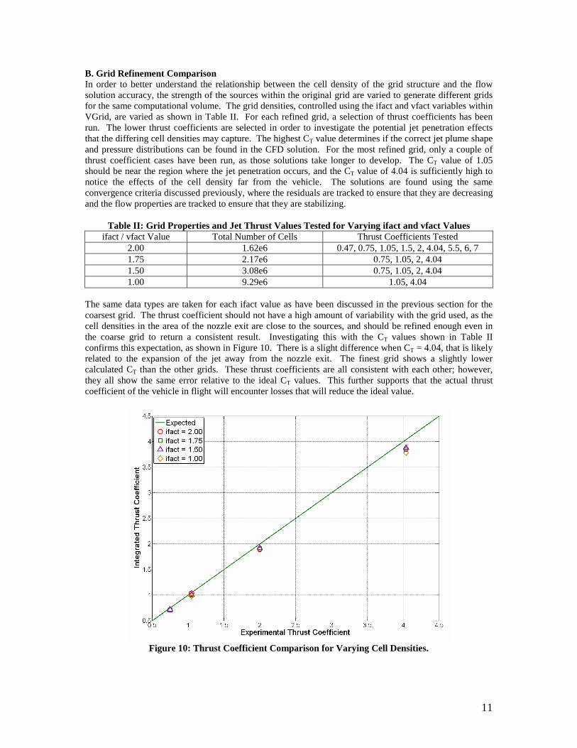
B. Grid Refinement Comparison In order to better understand the relationship between the cell density of the grid structure and the flow solution accuracy, the strength of the sources within the original grid are varied to generate different grids for the same computational volume. The grid densities, controlled using the ifact and vfact variables within VGrid, are varied as shown in Table II. For each refined grid, a selection of thrust coefficients has been run. The lower thrust coefficients are selected in order to investigate the potential jet penetration effects that the differing cell densities may capture. The highest CT value determines if the correct jet plume shape and pressure distributions can be found in the CFD solution. For the most refined grid, only a couple of thrust coefficient cases have been run, as those solutions take longer to develop. The CT value of 1.05 should be near the region where the jet penetration occurs, and the CT value of 4.04 is sufficiently high to notice the effects of the cell density far from the vehicle. The solutions are found using the same convergence criteria discussed previously, where the residuals are tracked to ensure that they are decreasing and the flow properties are tracked to ensure that they are stabilizing.

Table II: Grid Properties and Jet Thrust Values Tested for Varying ifact and vfact Values ifact / vfact Value Total Number of Cells Thrust Coefficients Tested

2.00 1.62e6 0.47, 0.75, 1.05, 1.5, 2, 4.04, 5.5, 6, 7 1.75 2.17e6 0.75, 1.05, 2, 4.04 1.50 3.08e6 0.75, 1.05, 2, 4.04 1.00 9.29e6 1.05, 4.04

The same data types are taken for each ifact value as have been discussed in the previous section for the coarsest grid. The thrust coefficient should not have a high amount of variability with the grid used, as the cell densities in the area of the nozzle exit are close to the sources, and should be refined enough even in the coarse grid to return a consistent result. Investigating this with the CT values shown in Table II confirms this expectation, as shown in Figure 10. There is a slight difference when CT = 4.04, that is likely related to the expansion of the jet away from the nozzle exit. The finest grid shows a slightly lower calculated CT than the other grids. These thrust coefficients are all consistent with each other; however, they all show the same error relative to the ideal CT values. This further supports that the actual thrust coefficient of the vehicle in flight will encounter losses that will reduce the ideal value.

Figure 10: Thrust Coefficient Comparison for Varying Cell Densities.

12

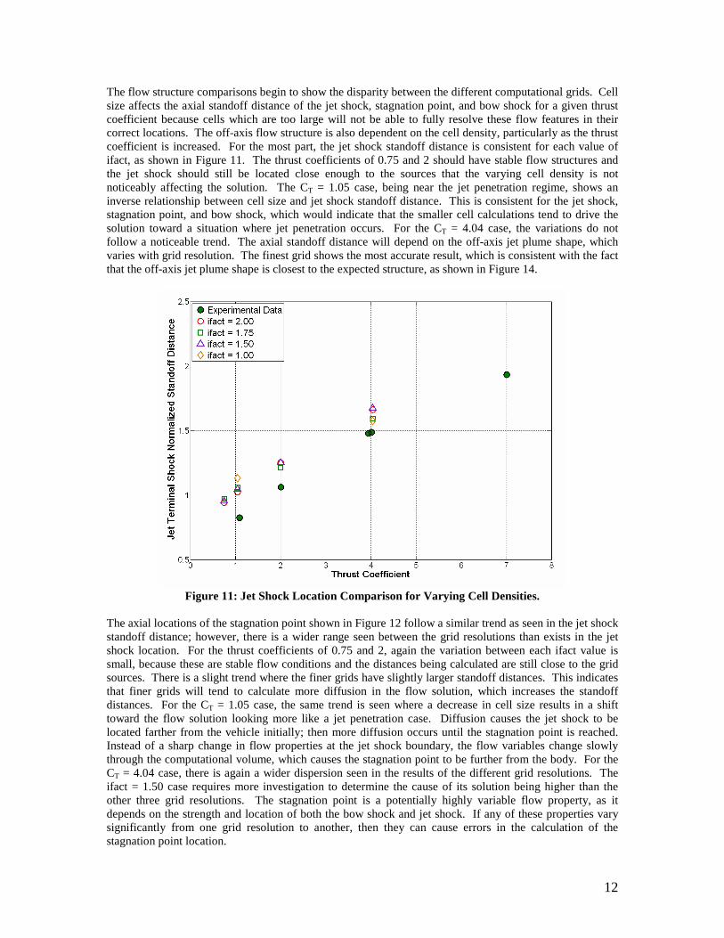
The flow structure comparisons begin to show the disparity between the different computational grids. Cell size affects the axial standoff distance of the jet shock, stagnation point, and bow shock for a given thrust coefficient because cells which are too large will not be able to fully resolve these flow features in their correct locations. The off-axis flow structure is also dependent on the cell density, particularly as the thrust coefficient is increased. For the most part, the jet shock standoff distance is consistent for each value of ifact, as shown in Figure 11. The thrust coefficients of 0.75 and 2 should have stable flow structures and the jet shock should still be located close enough to the sources that the varying cell density is not noticeably affecting the solution. The CT = 1.05 case, being near the jet penetration regime, shows an inverse relationship between cell size and jet shock standoff distance. This is consistent for the jet shock, stagnation point, and bow shock, which would indicate that the smaller cell calculations tend to drive the solution toward a situation where jet penetration occurs. For the CT = 4.04 case, the variations do not follow a noticeable trend. The axial standoff distance will depend on the off-axis jet plume shape, which varies with grid resolution. The finest grid shows the most accurate result, which is consistent with the fact that the off-axis jet plume shape is closest to the expected structure, as shown in Figure 14.

Figure 11: Jet Shock Location Comparison for Varying Cell Densities.

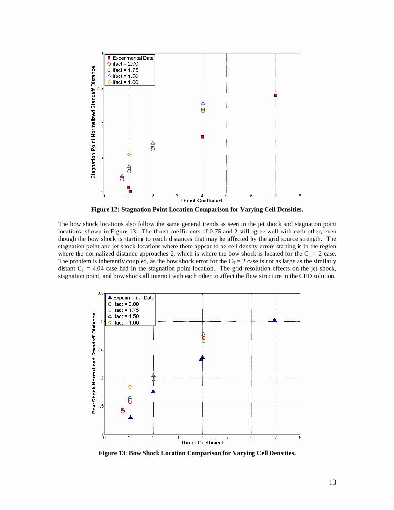
The axial locations of the stagnation point shown in Figure 12 follow a similar trend as seen in the jet shock standoff distance; however, there is a wider range seen between the grid resolutions than exists in the jet shock location. For the thrust coefficients of 0.75 and 2, again the variation between each ifact value is small, because these are stable flow conditions and the distances being calculated are still close to the grid sources. There is a slight trend where the finer grids have slightly larger standoff distances. This indicates that finer grids will tend to calculate more diffusion in the flow solution, which increases the standoff distances. For the CT = 1.05 case, the same trend is seen where a decrease in cell size results in a shift toward the flow solution looking more like a jet penetration case. Diffusion causes the jet shock to be located farther from the vehicle initially; then more diffusion occurs until the stagnation point is reached. Instead of a sharp change in flow properties at the jet shock boundary, the flow variables change slowly through the computational volume, which causes the stagnation point to be further from the body. For the CT = 4.04 case, there is again a wider dispersion seen in the results of the different grid resolutions. The ifact = 1.50 case requires more investigation to determine the cause of its solution being higher than the other three grid resolutions. The stagnation point is a potentially highly variable flow property, as it depends on the strength and location of both the bow shock and jet shock. If any of these properties vary significantly from one grid resolution to another, then they can cause errors in the calculation of the stagnation point location.

13

Figure 12: Stagnation Point Location Comparison for Varying Cell Densities.

The bow shock locations also follow the same general trends as seen in the jet shock and stagnation point locations, shown in Figure 13. The thrust coefficients of 0.75 and 2 still agree well with each other, even though the bow shock is starting to reach distances that may be affected by the grid source strength. The stagnation point and jet shock locations where there appear to be cell density errors starting is in the region where the normalized distance approaches 2, which is where the bow shock is located for the CT = 2 case. The problem is inherently coupled, as the bow shock error for the CT = 2 case is not as large as the similarly distant CT = 4.04 case had in the stagnation point location. The grid resolution effects on the jet shock, stagnation point, and bow shock all interact with each other to affect the flow structure in the CFD solution.

Figure 13: Bow Shock Location Comparison for Varying Cell Densities.

14

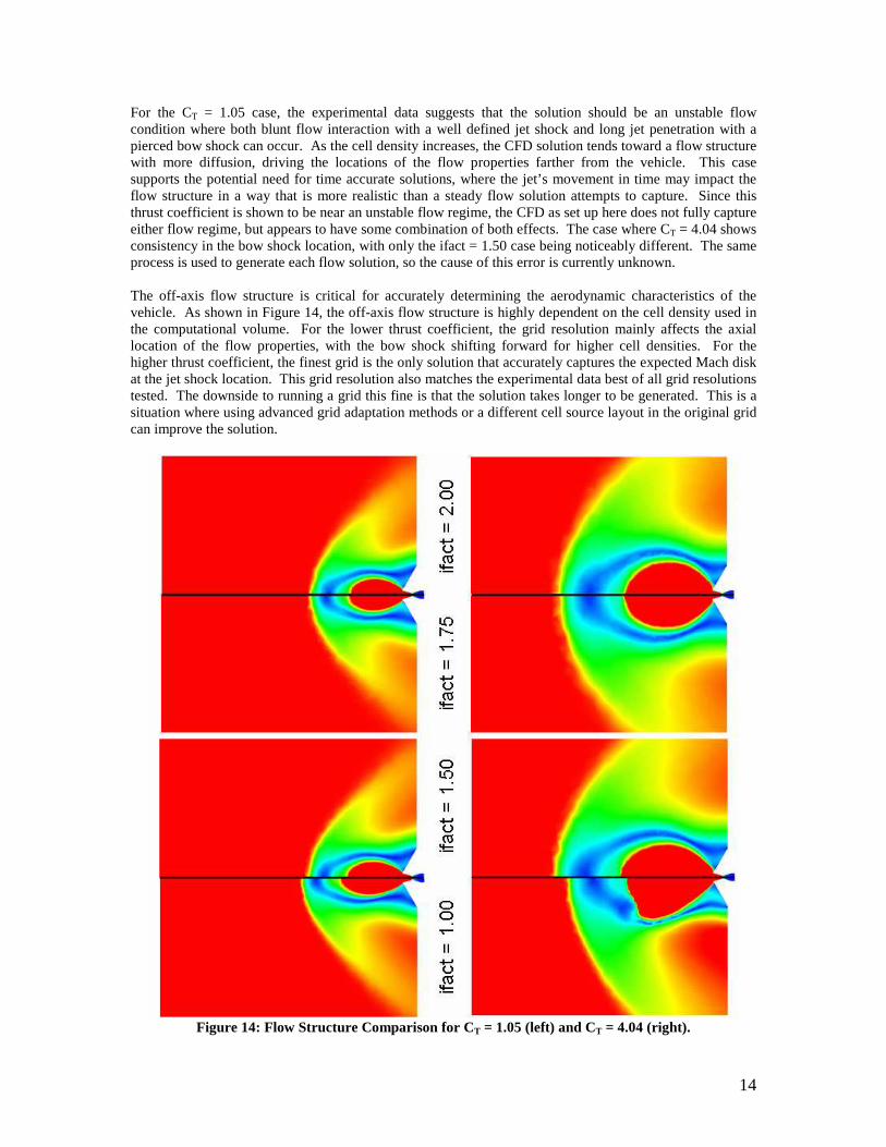
For the CT = 1.05 case, the experimental data suggests that the solution should be an unstable flow condition where both blunt flow interaction with a well defined jet shock and long jet penetration with a pierced bow shock can occur. As the cell density increases, the CFD solution tends toward a flow structure with more diffusion, driving the locations of the flow properties farther from the vehicle. This case supports the potential need for time accurate solutions, where the jet’s movement in time may impact the flow structure in a way that is more realistic than a steady flow solution attempts to capture. Since this thrust coefficient is shown to be near an unstable flow regime, the CFD as set up here does not fully capture either flow regime, but appears to have some combination of both effects. The case where CT = 4.04 shows consistency in the bow shock location, with only the ifact = 1.50 case being noticeably different. The same process is used to generate each flow solution, so the cause of this error is currently unknown. The off-axis flow structure is critical for accurately determining the aerodynamic characteristics of the vehicle. As shown in Figure 14, the off-axis flow structure is highly dependent on the cell density used in the computational volume. For the lower thrust coefficient, the grid resolution mainly affects the axial location of the flow properties, with the bow shock shifting forward for higher cell densities. For the higher thrust coefficient, the finest grid is the only solution that accurately captures the expected Mach disk at the jet shock location. This grid resolution also matches the experimental data best of all grid resolutions tested. The downside to running a grid this fine is that the solution takes longer to be generated. This is a situation where using advanced grid adaptation methods or a different cell source layout in the original grid can improve the solution.

Figure 14: Flow Structure Comparison for CT = 1.05 (left) and CT = 4.04 (right).

15

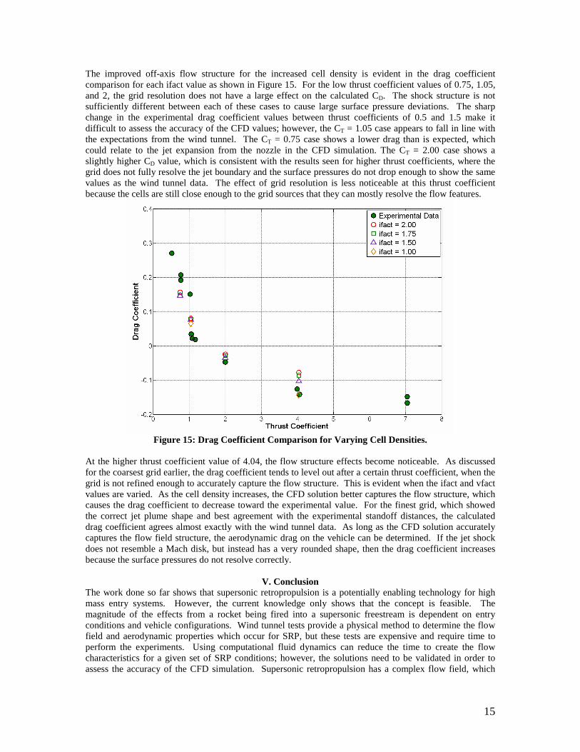
The improved off-axis flow structure for the increased cell density is evident in the drag coefficient comparison for each ifact value as shown in Figure 15. For the low thrust coefficient values of 0.75, 1.05, and 2, the grid resolution does not have a large effect on the calculated CD. The shock structure is not sufficiently different between each of these cases to cause large surface pressure deviations. The sharp change in the experimental drag coefficient values between thrust coefficients of 0.5 and 1.5 make it difficult to assess the accuracy of the CFD values; however, the CT = 1.05 case appears to fall in line with the expectations from the wind tunnel. The CT = 0.75 case shows a lower drag than is expected, which could relate to the jet expansion from the nozzle in the CFD simulation. The CT = 2.00 case shows a slightly higher CD value, which is consistent with the results seen for higher thrust coefficients, where the grid does not fully resolve the jet boundary and the surface pressures do not drop enough to show the same values as the wind tunnel data. The effect of grid resolution is less noticeable at this thrust coefficient because the cells are still close enough to the grid sources that they can mostly resolve the flow features.

Figure 15: Drag Coefficient Comparison for Varying Cell Densities.

At the higher thrust coefficient value of 4.04, the flow structure effects become noticeable. As discussed for the coarsest grid earlier, the drag coefficient tends to level out after a certain thrust coefficient, when the grid is not refined enough to accurately capture the flow structure. This is evident when the ifact and vfact values are varied. As the cell density increases, the CFD solution better captures the flow structure, which causes the drag coefficient to decrease toward the experimental value. For the finest grid, which showed the correct jet plume shape and best agreement with the experimental standoff distances, the calculated drag coefficient agrees almost exactly with the wind tunnel data. As long as the CFD solution accurately captures the flow field structure, the aerodynamic drag on the vehicle can be determined. If the jet shock does not resemble a Mach disk, but instead has a very rounded shape, then the drag coefficient increases because the surface pressures do not resolve correctly.

V. Conclusion The work done so far shows that supersonic retropropulsion is a potentially enabling technology for high mass entry systems. However, the current knowledge only shows that the concept is feasible. The magnitude of the effects from a rocket being fired into a supersonic freestream is dependent on entry conditions and vehicle configurations. Wind tunnel tests provide a physical method to determine the flow field and aerodynamic properties which occur for SRP, but these tests are expensive and require time to perform the experiments. Using computational fluid dynamics can reduce the time to create the flow characteristics for a given set of SRP conditions; however, the solutions need to be validated in order to assess the accuracy of the CFD simulation. Supersonic retropropulsion has a complex flow field, which

16

requires the CFD code to be capable of calculating many different flow situations. Creating a solution which is accurate in all aspects of the flow requires a grid capable of dealing with shocks located at varying distances from the vehicle and the expanding flow from the nozzle. Each of these properties requires a certain level of grid refinement in order to resolve properly in the CFD solution. For a single central nozzle, thrust coefficients less than 1 tend to be independent of the grid resolutions investigated in this study. The flow field is stable, and the shocks are close enough to the body that the grid is sufficiently fine to capture the flow structures. The surface pressure distributions and the aerodynamic drag coefficients are in agreement with the experimental results available. For a thrust coefficient of 1.05, the flow structure is unstable, with both blunt flow interaction and long jet penetration regimes seen in the wind tunnel experiments. This instability is not completely captured in the CFD solution; however, the surface pressure distribution does fall between that of the two expected flow regimes. Investigation of the flow properties in the CFD solution seems to indicate that the tendency of a steady flow is to capture some of both potential flow regimes. The shock is still relatively close to the body; however, there is significant diffusion which causes the jet plume to elongate and push the bow shock further from the body. The CFD data is consistent with the expectations from the wind tunnel experiments, but capturing each flow regime seen in testing requires more detailed computational work. For higher thrust coefficients, where the flow field structure should be stable, the computational grid begins to affect the CFD solution. The cell size must be small enough to accurately capture the jet shock, stagnation point, and bow shock caused by the expanding nozzle flow. If the cells are too large, then the axial locations of the flow properties can be consistently determined; however, the off-axis shape of the jet plume will not match schlieren imagery taken in the wind tunnel. This mismatch in the off-axis structure affects the surface pressure distribution on the vehicle, which causes the calculated drag coefficient to level out at a higher value than is expected as the thrust coefficient is increased. Varying the grid resolution shows that the correct flow properties can be captured, indicating that the CFD code is capable of accurately modeling high thrust coefficient supersonic retropropulsion conditions. As the flow structure becomes more accurate in the CFD simulation, the drag coefficient will have better agreement. When the jet plume is calculated to terminate in a Mach disk, which matches the expectations from the wind tunnel experiments, the drag coefficient becomes consistent with the wind tunnel data.

VI. Future Work There are two main areas where the study of supersonic retropropulsion can be improved. One is that the computational methods and investigations need to be expanded. As shown in this study, for a static grid to be capable of modeling a wide range of jet conditions, the cells need to be refined throughout a large portion of the computational volume. This increases the grid size, which lengthens the computational time. One way to create a robust grid which has larger cells is to use active grid refinement while the solution develops. Fun3D has a refinement package, which is capable of shifting the cells such that coarser grids are still capable of resolving the flow features accurately. A brief investigation of grid refinement within Fun3D for the SRP problem shows that the tendency of the mesh movement via spring analogy [8] is to move the cells into the nozzle. The algorithm wants to better resolve the boundary layer within the expanding nozzle flow, instead of concentrating on the shock boundaries away from the vehicle. Determining the best method to resolve the flow field properties would allow for quicker computation of the SRP conditions. In addition to the actual CFD methodology, the vehicle configurations which are computationally solved need to be expanded. The flow properties for the single nozzle configuration investigated in this study are somewhat different from those seen in the peripheral configurations. Since these types of vehicle setups show promise in enhancing the drag performance of the vehicle [2], [5], being able to accurately capture the flow field and aerodynamic properties associated with these configurations is necessary. Some of the same computational ideas that are useful in the single nozzle configuration can be applied to the peripheral configurations, such as knowing where sources need to be located to correctly define the initial grid refinement. The other area where the study of SRP can be improved is that of the experimental data. The current data comes from experiments performed many years ago. While the time lag doesn’t affect the numbers in the

17

data, it does affect the knowledge about how the data was taken. It is important for CFD validation to know the circumstances under which the schlieren imagery and pressure distributions were taken in order to understand how well the CFD solution matches the physical system. Data on the unsteadiness seen in the physical model, the time accurate variation of the flow field, and the conditions under which the tests are performed would all enable the CFD environment to be better suited for accurately matching the flow properties. Some of this data is reported in the previous experiments, but having current data where the experiment can be set up to provide all of the data which is useful to initializing a CFD solution would benefit the advancement of SRP research. Instead of basing the nozzle properties off ideal expansion through a nozzle with no losses, the actual wind tunnel nozzle pressure can be measured and used in the computational environment to set up more accurate initial conditions. Having time histories of the flow field and surface pressure distributions in the physical model will determine if steady CFD solutions are falling within the expected range of locations for the shocks, or if a time accurate CFD solution is required to accurately capture the flow interactions.

VII. References [1] Braun, R. D., and Manning, R. M., “Mars Exploration Entry, Descent, and Landing Challenges,”

Journal of Spacecraft and Rockets, Vol. 44, No. 2, pp. 310-323, March-April 2007. [2] Korzun, A. M., Cruz, J. R., and Braun, R. D., “A Survey of Supersonic Retropropulsion

Technology for Mars Entry, Descent, and Landing,” 2008 IEEE Aerospace Conference, IEEEAC 1246, Big Sky, MT, March 2008.

[3] McGhee, R. J., “Effects of a Retronozzle Located at the Apex of a 140° Blunt Cone at Mach

Numbers of 3.00, 4.50, and 6.00,” NASA TN D-6002, January 1971. [4] Daso, E. O., Pritchett, V. E., Wang, T. S., “The Dynamics of Shock Dispersion and Interactions in

Supersonic Freestreams with Counterflowing Jets,” 45th AIAA Aerospace Sciences Meeting, AIAA 2007-1423, Reno, Nevada, January 2007.

[5] Jarvinen, P. O., and Adams, R. H., “The Aerodynamic Characteristics of Large Angled Cones

with Retrorockets,” NASA Contract No. NAS 7-576, February 1970. [6] “GridTool: A Surface Modeling and Grid Generation Tool,” NASA Langley Research Center,

May 2005, http://geolab.larc.nasa.gov/GridTool/ [retrieved June 2008]. [7] “VGRID Unstructured Grid Generation,” August 2003, http://tetruss.larc.nasa.gov/vgrid/

[retrieved June 2008]. [8] “Fun3D Manual,” May 2009, http://fun3d.larc.nasa.gov [retrieved June 2008]. [9] Krist, S. L., Biedron, R. T., and Rumsey, C. L., “CFL3D User’s Manual (Version 5.0),” 2nd ed.,

September 1997, pp. 53-56, also NASA TM-1998-208444, June 1998, http://cfl3d.larc.nasa.gov/Cfl3dv6/cfl3dv6.html [retrieved July 2008].

18

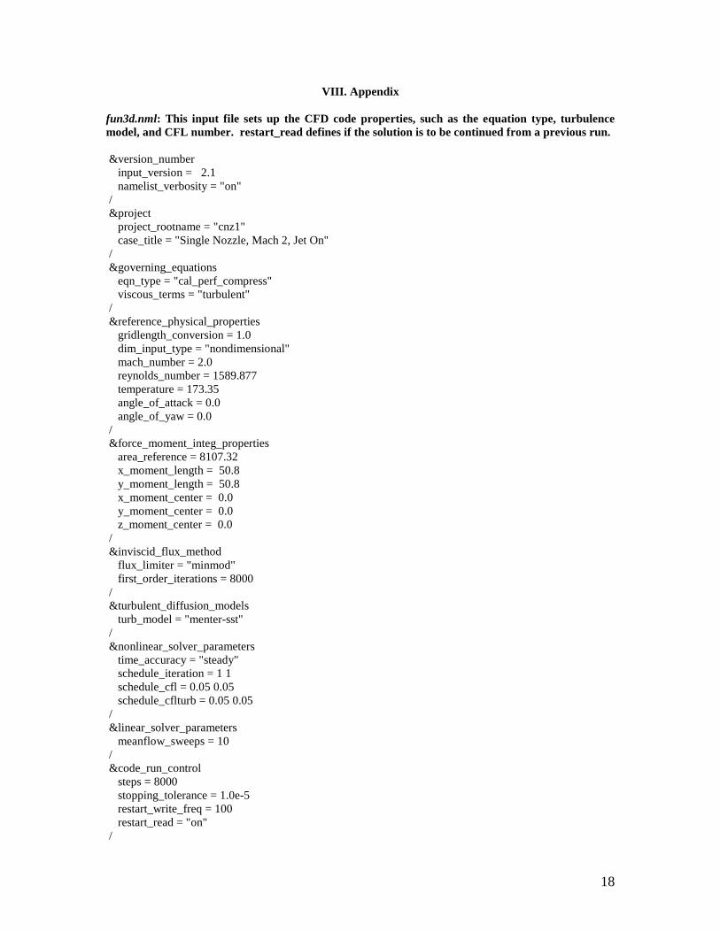
VIII. Appendix fun3d.nml: This input file sets up the CFD code properties, such as the equation type, turbulence model, and CFL number. restart_read defines if the solution is to be continued from a previous run. &version_number input_version = 2.1 namelist_verbosity = "on" / &project project_rootname = "cnz1" case_title = "Single Nozzle, Mach 2, Jet On" / &governing_equations eqn_type = "cal_perf_compress" viscous_terms = "turbulent" / &reference_physical_properties gridlength_conversion = 1.0 dim_input_type = "nondimensional" mach_number = 2.0 reynolds_number = 1589.877 temperature = 173.35 angle_of_attack = 0.0 angle_of_yaw = 0.0 / &force_moment_integ_properties area_reference = 8107.32 x_moment_length = 50.8 y_moment_length = 50.8 x_moment_center = 0.0 y_moment_center = 0.0 z_moment_center = 0.0 / &inviscid_flux_method flux_limiter = "minmod" first_order_iterations = 8000 / &turbulent_diffusion_models turb_model = "menter-sst" / &nonlinear_solver_parameters time_accuracy = "steady" schedule_iteration = 1 1 schedule_cfl = 0.05 0.05 schedule_cflturb = 0.05 0.05 / &linear_solver_parameters meanflow_sweeps = 10 / &code_run_control steps = 8000 stopping_tolerance = 1.0e-5 restart_write_freq = 100 restart_read = "on" /

19

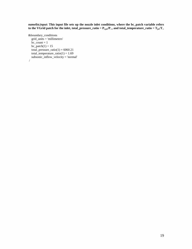
namelist.input: This input file sets up the nozzle inlet conditions, where the bc_patch variable refers to the VGrid patch for the inlet, total_pressure_ratio = Pt,jet/P∞, and total_temperature_ratio = Tjet/T∞ &boundary_conditions grid_units = 'millimeters' bc_count = 1 bc_patch(1) = 15 total_pressure_ratio(1) = 6060.21 total_temperature_ratio(1) = 1.69 subsonic_inflow_velocity = 'normal' /