HAL Id: hal-01383256https://hal.archives-ouvertes.fr/hal-01383256

Preprint submitted on 18 Oct 2016

HAL is a multi-disciplinary open accessarchive for the deposit and dissemination of sci-entific research documents, whether they are pub-lished or not. The documents may come fromteaching and research institutions in France orabroad, or from public or private research centers.

L’archive ouverte pluridisciplinaire HAL, estdestinée au dépôt et à la diffusion de documentsscientifiques de niveau recherche, publiés ou non,émanant des établissements d’enseignement et derecherche français ou étrangers, des laboratoirespublics ou privés.

Computational fluid dynamics in the upper airway:comparison between different models and experimentaldata for a simplified geometry with major obstructionFatemeh Heravi, Mohammad Nazari, Franz Chouly, Pascal Perrier, Yohan

Payan

To cite this version:Fatemeh Heravi, Mohammad Nazari, Franz Chouly, Pascal Perrier, Yohan Payan. Computationalfluid dynamics in the upper airway: comparison between different models and experimental data fora simplified geometry with major obstruction. 2016. �hal-01383256�

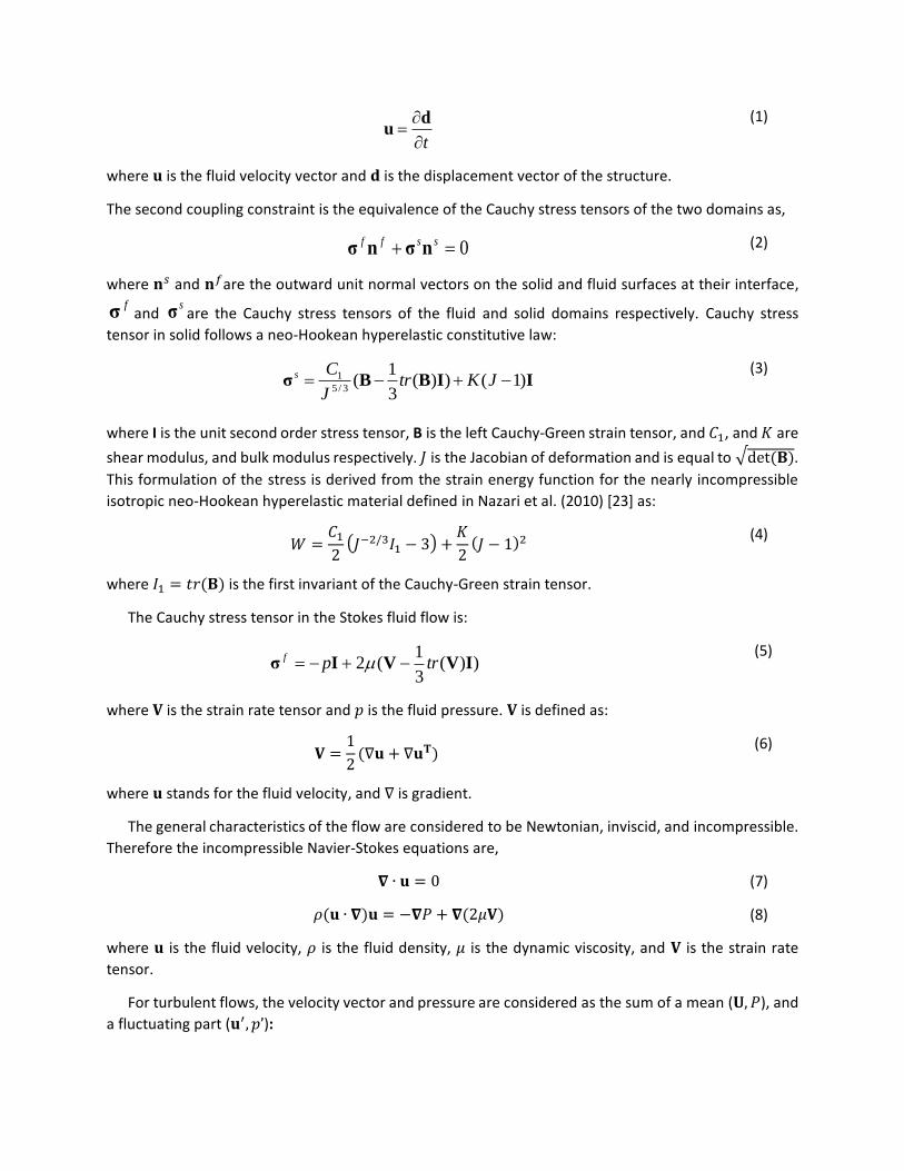
Computational fluid dynamics in the upper airway: comparison between

different models and experimental data for a simplified geometry with major

obstruction

Fatemeh Entezari Heravi1, Mohammad Ali Nazari1, Franz Chouly2, Pascal Perrier3 and Yohan

Payan4

1School of Mechanical Engineering, College of Engineering, University of Tehran, Tehran, Iran 2Laboratoire de Mathématiques de Besançon, UBFC, F-25000 Besançon cedex, France 3Univ. Grenoble Alpes & CNRS, Gipsa-lab, F-38000 Grenoble, France 4Univ. Grenoble Alpes & CNRS, TIMC-IMAG,F-38000 Grenoble, France

Abstract

The present study aims at comparing different computational models used for simulating the fluid-

structure interaction within an in-vitro setup resembling simplified major obstruction of pharyngeal

airway. Due to the nature of the problem, i.e. air flow passing over a deformable latex surface, a fully

coupled fluid-structure interaction algorithm is used. A comparison is made between two finite element

models for the solid domain, one using shell and the other using volume elements. The material

properties of these models follow a hyperelastic behavior. For the fluid part, laminar and various

turbulence models such as standard 𝑘 − 𝜀, Shear Stress Transport, SSG Reynolds Stress and BSL

Reynolds Stress are compared. We evaluate the efficiency of the models and how close to the

experimental data are their results. The predictions of the structural model containing volume elements

showed better consistency with the experimental data. In addition, the results obtained with the

standard 𝑘 − 𝜀 turbulence model were the least deviated among all turbulence models.

Keywords: Fully coupled fluid-structure interaction; pharyngeal airway; finite element method; laminar

fluid flow; turbulent fluid flow.

1 Introduction

Numerical modelling of flows in human body is of great importance. Various studies have been focusing

on the airflow along the respiratory system, particularly in the upper airway. Some of them have

modeled only fluid flow assuming rigid boundaries. For instance, Wang et al. (2009) [1] have predicted

the airflow along the upper airway during a whole respiratory cycle using 𝑘 − 𝜀 turbulence model for

the transient analysis. In Mylavarapu et al. (2009) [2], various turbulence models such as unsteady Large

Eddy Simulation (LES) model and some of the steady Reynolds-Averaged Navier-Stokes (RANS) models,

i.e. 𝑘 − 𝜀, 𝑘 − 𝜔, 𝑘 − 𝜔-based Shear Stress Transport, and Spallart-Alarmas models, are compared on

the basis of flow computation in the upper airway. In the aforementioned study, the peak expiratory

flow rate goes through the upper airway and the regions of minimum negative pressure are determined.

These regions are those where the obstruction is most likely to occur. The characteristics of the flow

pattern in the inspiratory phase are discussed in Sung et al. (2006) [3] and the regions prone for

obstruction in nasal cavity and in the pharynx are determined using RNG 𝑘 − 𝜀 model, which is a

modified version of the standard 𝑘 − 𝜀 model that takes account of the contribution of different

turbulence scales rather than considering only the length scale. The Spalart-Allmaras model is preferred

by Nithiarasu et al. (2008) [4] and they claim that this model is commonplace for incompressible flow

calculations. Their study resulted in specifying the regions of minimum negative pressure by studying

the steady inspiratory flow. In Lucey et al. (2010) [5], the Shear Stress Transport Turbulence (SST) model

is employed to predict the airflow pattern during the inhalation phase of the respiratory cycle within a

3D pharyngeal geometry reconstructed from the data of optical coherence tomography (OCT) which

could capture multi-sectional images of a tissue structure (Fujimoto (2000) [6]). Moreover, in this study,

the effect of different wall positions is taken into account through a change of the initial rigid wall

geometry. Based on a brief comparison of the results of laminar flow model, 𝑘 − 𝜀 model, and 𝑘 − 𝜔

SST turbulence model they concluded that the SST model would be more appropriate than the other

three. The response of the upper airway to the mandibular advancement splint in treating major

obstructions of the airway is investigated in Zhao et al. (2013) [7]. In this study, the 𝑘 − 𝜔 based Shear

Stress Transport model is considered appropriate for the upper airway flow. The effect of nasal

obstruction in positive airway pressure treatment therapy is studied using Spalart-Allmaras model in

Wakayama et al. (2016) [8]. In Cisonni et al. (2013) [9] the pressure drop in the velopharynx of subjects

with and without obstructions in the upper airway was computed using fluid flow simulations with 𝑘 −

𝜔 SST modeling on the anatomies constructed from optical coherence tomography (OCT).

The effect of fluid pressure on deformable parts of the upper airway has been studied in

Pelteret and Reddy (2014) [10] and Carrigy et al. 2015 [11]. In Pelteret and Reddy (2014) [10] the fluid

pressure changes sinusoidally to represent the effect of inhaling and exhaling but its magnitude is

considered uniform except in the mouth region where it decreases linearly from the tip of tongue to the

pharyngeal part of the tongue to model the inhaling through the mouth. The simulation is then

completed using FEM analysis. In Carrigy et al. (2015) [11] a uniform negative pressure is applied on the

whole model to study the effect of area changes in velar and oral parts. Then the aforementioned

authors determined the most appropriate Young’s Moduli of the muscles and the adipose tissues

assuming a linear elastic model.

In other studies the assumption of rigid boundaries has been replaced by a more realistic one.

There are several works where both the airflow and its deformable pathway are modeled using fluid-

structure interaction (FSI) method. In Huang et al. (2008) [12] a two-dimensional finite-element model

of the upper airway is examined under laminar flow conditions taking into account the muscle’s active

properties. A 2D FSI simulation is carried out upon a simplified geometry for both normal and abnormal

pharyngeal airways in Wang et al. (2009) [1]. In Chouly et al. (2008) [13] the FSI method is used for

coupling a 3D deformable solid model and a 2D fluid model of the expiratory flow in the upper airway

during major obstructions. In this study, flow features are analyzed with Reduced Navier-Stokes/Prandtl

(RNS/P) equations which are described in Lagrée and Lorthois (2005) [14]. These equations are also used

for the analysis of the flow in a 2D model of the oropharynx in Chouly et al. (2006) [15]. A 3D model of

the expiratory airflow is simulated with fully coupled FSI method in Rasani et al. (2011) [16]. 𝑘 − 𝜔

based Shear Stress Transport model is adopted for this study. In Heil (2003) [17], a review is published

that presents numerous models used for investigating general characteristics of airflow in interaction

with soft tissues throughout the human body. These models range from zero-equation models to three-

dimensional Navier-Stokes simulations. This publication emphasizes the necessity and importance of

fully-coupled approaches for dealing with such problem. Such a fully coupled FSI simulation is used by

Wang et al. (2012) [18] for determining the efficiency of nasal surgery, where the standard 𝑘 − 𝜔

turbulence model is employed for simulating the flow domain. The same is done by Zhao et al. (2013)

[19] for the study on mandibular advancement method, using the 𝑘 − 𝜔 based Shear Stress Transport.

The deformation along the entire upper airway is studied by transient flow analysis coupled with linear

structural analysis in Kim et al. (2015) [20] using Large Eddy Simulation model for the transient analysis

of the fluid domain. In Pirnar et al. (2015) [21] both soft palate flutter and the airway narrowing are

simulated through fully coupled FSI method. In all of these fluid-structure interaction studies, the solid

domain is considered linearly elastic.

Given the diversity of the models available for simulating fluid-structure interaction in the upper

airways, and the variety of their predictions in the context of the study of the sleep apnea syndrome, a

precise and quantitative assessment of these different approaches is needed. In this aim, we propose to

take the measures carried out by Chouly et al. (2008) with a replica of the pharyngeal airway as reliable

reference data to which the predictions of the models will be precisely and quantitatively compared.

The advantage of using these experimental results is that they were obtained in controlled conditions

through precise measurement techniques which could not be achieved while working with patient-

specific data. In order for increasing the accuracy of the results, a fully coupled method is chosen as the

fluid-structure coupling algorithm, and hyperelastic material properties are assigned to the solid

domain. In previous works Chouly et al. (2008) [13] using RNS/P equations provided predictions of the

pressure drop within the constriction of the pharyngeal replica, and of the flow-induced deformation,

that fitted well the experimental data. Nevertheless, in order to go further and carry out later on

simulations from real and complex patient-specific geometries, other fluid flow models should be

considered. Indeed RNS/P equations are mostly limited to simple 2D geometries and induce numerical

difficulties in case of heavy recirculation after the constriction. Therefore, complete 3D Navier-Stokes

equations with laminar or turbulent closures should be considered, as they are now available in

standard finite element packages such as ANSYS/FLUENT(TM). In addition, since various turbulent

models are provided in ANSYS/CFX 15.0 and are used in biomedical simulations, their predictive

performance and accuracy for studying such a complex phenomenon need to be compared using

relevant experimental data. The efficiencies of two different finite element models for the solid domain

are examined; one containing shell elements and, the other, volume elements. Some of the most

commonplace flow models, i.e. laminar, standard 𝑘 − 𝜀, Shear Stress Transport, and BSL and SSG

Reynolds Stress models, are compared to each other in this study (“BSL” and “SSG” stand for “Baseline”

and “Speziale, Sarkar, Gatski” respectively). The pressure value at the point where the constriction is the

narrowest is used as a key variable for comparing the results of the numerical models and the

experimental results reported in Chouly et al. (2008) [22].

2 Theoretical assumptions and materials

2.1 Governing Equations

For appropriate simulations of fluid-structure interaction problems such as highly deformable tissues

interacting with turbulent flows, an iterative fully coupled transient algorithm is suggested where fluid

and solid equations are solved by separate solvers. Especially having large deformations in solid domain

would affect the boundary conditions of the fluid flow. In this algorithm, two constraints are set at the

interface of the fluid and solid domains for coupling. The first constraint is the relationship between the

displacement in the solid domain and the fluid velocity at each interface node as:

t

du

(1)

where 𝐮 is the fluid velocity vector and 𝐝 is the displacement vector of the structure.

The second coupling constraint is the equivalence of the Cauchy stress tensors of the two domains as,

0 ssff nσnσ (2)

where 𝐧𝑠 and 𝐧𝑓are the outward unit normal vectors on the solid and fluid surfaces at their interface, fσ and

sσ are the Cauchy stress tensors of the fluid and solid domains respectively. Cauchy stress

tensor in solid follows a neo-Hookean hyperelastic constitutive law:

IIBBσ )1())(3

1(

3/5

1 JKtrJ

Cs (3)

where I is the unit second order stress tensor, B is the left Cauchy-Green strain tensor, and 𝐶1, and 𝐾 are

shear modulus, and bulk modulus respectively. 𝐽 is the Jacobian of deformation and is equal to √det(𝐁).

This formulation of the stress is derived from the strain energy function for the nearly incompressible

isotropic neo-Hookean hyperelastic material defined in Nazari et al. (2010) [23] as:

𝑊 =𝐶12(𝐽−2/3𝐼1 − 3) +

𝐾

2(𝐽 − 1)2

(4)

where 𝐼1 = 𝑡𝑟(𝐁) is the first invariant of the Cauchy-Green strain tensor.

The Cauchy stress tensor in the Stokes fluid flow is:

))(3

1(2 IVVIσ trpf

(5)

where𝐕 is the strain rate tensor and 𝑝 is the fluid pressure. 𝐕 is defined as:

𝐕 =1

2(∇𝐮 + ∇𝐮𝐓)

(6)

where 𝐮 stands for the fluid velocity, and ∇ is gradient.

The general characteristics of the flow are considered to be Newtonian, inviscid, and incompressible.

Therefore the incompressible Navier-Stokes equations are,

𝛁 ∙ 𝐮 = 0 (7)

𝜌(𝐮 ∙ 𝛁)𝐮 = −𝛁𝑃 + 𝛁(2𝜇𝐕) (8)

where 𝐮 is the fluid velocity, 𝜌 is the fluid density, 𝜇 is the dynamic viscosity, and 𝐕 is the strain rate

tensor.

For turbulent flows, the velocity vector and pressure are considered as the sum of a mean (𝐔, 𝑃), and

a fluctuating part (𝐮′, 𝑝’):

𝐮 = 𝐔+ 𝐮′ (9 a)

p=P+p’ (9 b)

With Reynolds time averaging defined as,

𝐟̅ = limT→∞

1

𝑇∫ 𝐟(𝑠)𝑡+𝑇

𝑡

𝑑𝑠 (10)

and by applying this type of averaging on Eq. (7) and Eq. (8) using Eqs. (9), the Reynolds averaged

equation of mass conservation, and the Reynolds Averaged Navier-Stokes (RANS), are derived as:

𝛁 ∙ 𝐔 = 0 (11)

𝜌(𝐔 ∙ 𝛁)𝐔 = −𝛁𝑃 + 𝛁[2𝜇𝐕 − 𝜌𝝉] (12)

where 𝜌𝝉 is called Reynolds Stress tensor. The components of this tensor are equal to 𝜌𝐮′⨂𝐮′(⨂ stands

for the dyadic product of two vectors) and the way one defines it determines the type of the flow model

with which the simulation is to be done (Wilcox(1993) [24]). For laminar flow, this term would be zero,

because the velocity field is assumed to have no fluctuation in any direction. In turbulence modeling,

there are two major ways for defining this term. In the first way, the Eddy Viscosity model assumes that

Reynolds stresses are proportional to mean velocity gradients and are defined as:

𝜌𝐮′⨂𝐮′ = 𝜇𝑡𝐕 −2

3𝐈(𝜌𝑘)

(13)

where 𝑘 is the turbulence kinetic energy defined as 𝑘 =𝐮′∙𝐮′̅̅ ̅̅ ̅̅ ̅

𝟐, and 𝜇𝑡 is the eddy viscosity or turbulent

viscosity; in the 𝑘 − 𝜀 model and the Shear Stress Transport Model 𝜇𝑡 is respectively defined as:

𝜇𝑡 = 𝐶𝜇𝜌𝑘2

𝜀

(14)

𝜇𝑡 = 𝜌𝛼𝑘

max(𝛼𝜔, 𝑆𝐹)

(15)

where 𝐶𝜇 and 𝛼 are constant parameters, 𝜀 is the turbulence eddy dissipation rate, 𝜔 is the specific

dissipation rate, 𝑆 is an invariant of the strain rate matrix, and 𝐹 is a blending function. These variables

are defined trough the following equations:

𝜀 = 𝜈𝛁𝐮′: 𝛁𝐮′̅̅ ̅̅ ̅̅ ̅̅ ̅̅ ̅ (16)

𝜔 =𝜀

𝑘 (17)

𝐹 = tanh(𝑓2) (18)

where 𝑓 is defined as,

𝑓 = max(2√𝑘

𝛽𝜔𝑦,500𝜈

𝑦2𝜔)

(19)

where “:” shows double contraction of two second-order tensors, 𝛽 is a constant, 𝑦 is the distance to

the nearest wall, and 𝜈 is the kinematic viscosity.

The second common way for modeling Reynlods Stress Tensor term is called Reynolds Stress model.

It is based on solving transport equations for all Reynolds stress tensor components and the dissipation

rate. Two of the most commonplace methods of this type are SSG Reynolds Stress model and BSL

Reynolds Stress model whose formulations could be found in Eisfeld (2010) [25].

The simulation is conducted through three levels of iteration, (a) the field loop, used to converge

toward a solution for each field with the associated solver, (b) the coupling loop, used for exchanging

loads or displacements between the two fields, and, (c) the time loop which intends to make each step

move forward in time. Within each field loop, the governing equations of the flow, Eq. (7) and Eq. (8),

are solved for finding the value of pressure and velocity vector at nodes. During the coupling (stagger)

loop, the results of the fluid field solver are applied to the relevant nodes of the solid domain using Eq.

(2). The solid field solver computes the deformation of the structure and the results are applied on the

fluid interface with solid domain as a new set of boundary conditions during the coupling loop using Eq.

(1). This iterative coupling procedure continues until the convergence tolerance or the maximum

number of iterations is reached. For a steady-state FSI simulation the solution for fluid domain is quasi-

static and for solid domain is transient within each field loop (Gianopapa, 2004 [26]).

2.2 Material properties

We have seen above that the solid domain is considered to follow the neo-Hookean material model.

Solid domain is of latex material and its elastic parameters are 𝐸 = 1.68MPa and ν = 0.499 (Chouly et

al., 2008).

Linearization of Eq. (4) at initial point gives,

𝐶1 = 𝐸/3 (20)

And with the assumption of nearly incompressible material the material constants are given in Table 1.

Table 1 Constants of the neo-Hookean 𝑾 function

𝐾/2 (1/𝑃𝑎) 𝐶1 (𝑃𝑎)

7.1429𝑒 − 09 560000

The fluid material is set as air at 25℃ with 𝜌 = 1.185𝑘𝑔

𝑚3 and 𝜇 = 1.831 × 10−5𝑘𝑔

𝑚𝑠.

3 Finite Element Model

The geometry of the pharyngeal replica setup was created using the dimensions reported in Chouly et

al. (2008) (Fig. 1). The model is build up in ANSYS release 15. Fig. 2 represents the finite element model

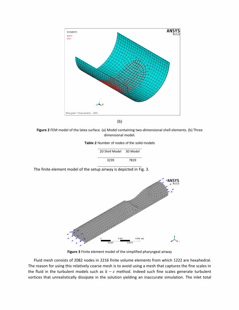
of the latex surface. The mesh in Fig. 2(a) consists of a layer of 8-node quadrilateral SHELL181 elements,

and the one in Fig. 2(b) consists of 20-node hexahedral SOLID186 elements along with 10-node SOLID

187 elements. The SOLID187 elements are distributed through the thickness and they count to 337 out

of 1760 total elements. The number of elements and nodes of these two models are given in Table 2.

The thickness of latex layer is 0.3𝑚𝑚. As shown, the latex surface is divided into two regions. The core

region is in interaction with the airflow and the surrounding region is attached to the rigid pipe. Water

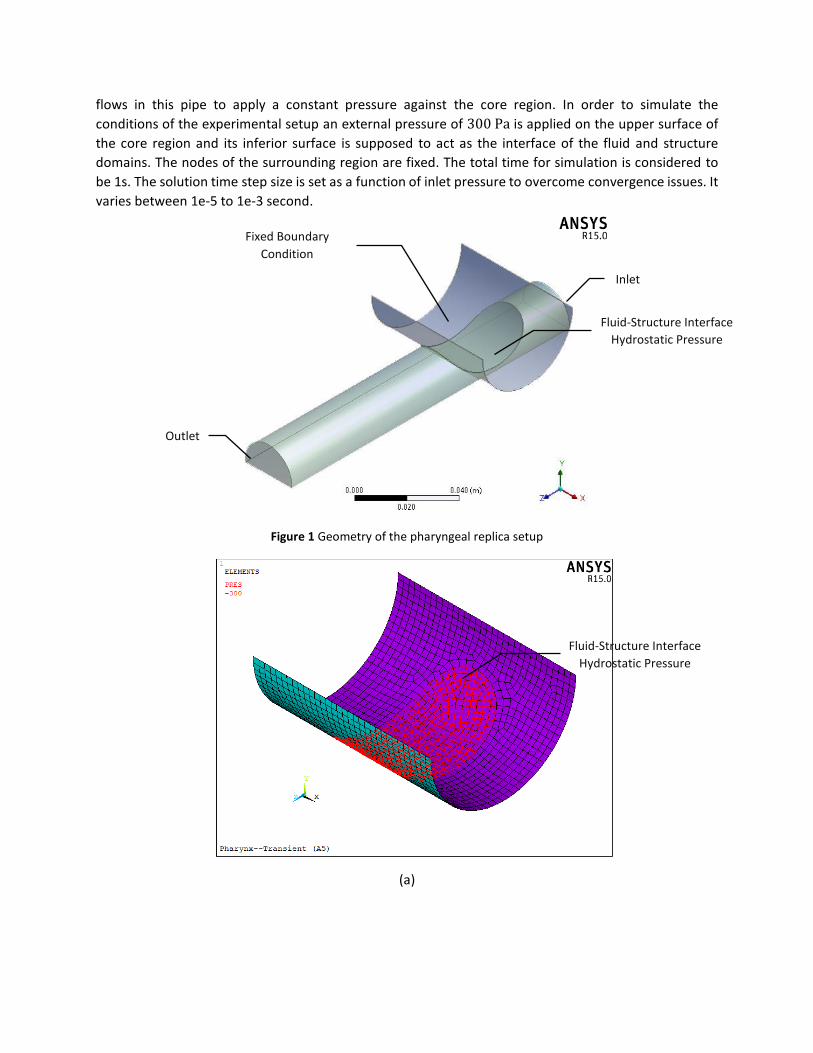
flows in this pipe to apply a constant pressure against the core region. In order to simulate the

conditions of the experimental setup an external pressure of 300Pa is applied on the upper surface of

the core region and its inferior surface is supposed to act as the interface of the fluid and structure

domains. The nodes of the surrounding region are fixed. The total time for simulation is considered to

be 1s. The solution time step size is set as a function of inlet pressure to overcome convergence issues. It

varies between 1e-5 to 1e-3 second.

Figure 1 Geometry of the pharyngeal replica setup

(a)

Fluid-Structure Interface

Hydrostatic Pressure

Inlet

Fixed Boundary

Condition

Outlet

Fluid-Structure Interface

Hydrostatic Pressure

(b)

Figure 2 FEM model of the latex surface. (a) Model containing two-dimensional shell elements. (b) Three

dimensional model.

Table 2 Number of nodes of the solid models

3D Model 2D Shell Model

7819 3239

The finite element model of the setup airway is depicted in Fig. 3.

Figure 3 Finite element model of the simplified pharyngeal airway

Fluid mesh consists of 2082 nodes in 2216 finite volume elements from which 1222 are hexahedral.

The reason for using this relatively coarse mesh is to avoid using a mesh that captures the fine scales in

the fluid in the turbulent models such as 𝑘 − 𝜀 method. Indeed such fine scales generate turbulent

vortices that unrealistically dissipate in the solution yielding an inaccurate simulation. The inlet total

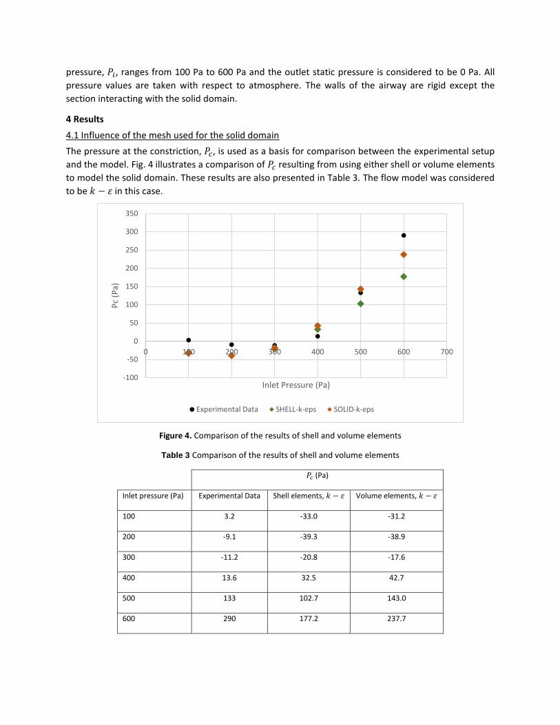
pressure, 𝑃𝑖, ranges from 100 Pa to 600 Pa and the outlet static pressure is considered to be 0 Pa. All

pressure values are taken with respect to atmosphere. The walls of the airway are rigid except the

section interacting with the solid domain.

4 Results

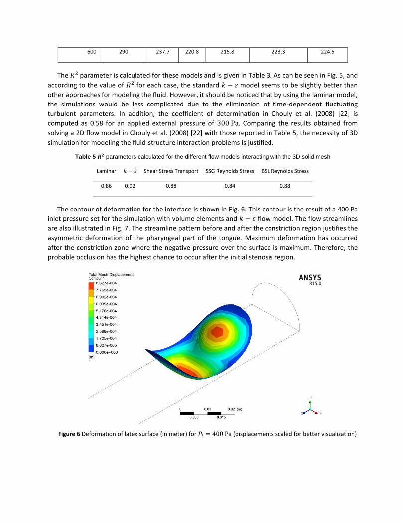
4.1 Influence of the mesh used for the solid domain

The pressure at the constriction, 𝑃𝑐, is used as a basis for comparison between the experimental setup

and the model. Fig. 4 illustrates a comparison of 𝑃𝑐 resulting from using either shell or volume elements

to model the solid domain. These results are also presented in Table 3. The flow model was considered

to be 𝑘 − 𝜀 in this case.

Figure 4. Comparison of the results of shell and volume elements

Table 3 Comparison of the results of shell and volume elements

𝑃𝑐 (Pa)

Volume elements, 𝑘 − 𝜀 Shell elements, 𝑘 − 𝜀 Experimental Data Inlet pressure (Pa)

-31.2 -33.0 3.2 100

-38.9 -39.3 -9.1 200

-17.6 -20.8 -11.2 300

42.7 32.5 13.6 400

143.0 102.7 133 500

237.7 177.2 290 600

-100

-50

0

50

100

150

200

250

300

350

0 100 200 300 400 500 600 700

Pc

(Pa)

Inlet Pressure (Pa)

Experimental Data SHELL-k-eps SOLID-k-eps

The coefficient of determination, 𝑅2, was computed as 0.92 for the model with volume elements,

and 0.78 for that with shell elements. Comparing these values, we observed a trend for the volume

element to work better for simulating such thin hyper-elastic surfaces interacting with the passage of

fluid flow.

4.2 Influence of the flow model

In Fig. 5, the value of 𝑃𝑐 is indicated vs. different values of inlet pressure using each one of the flow

models described in section 2.1. The three-dimensional structure is chosen for the solid domain in this

comparison. The results are also presented in Table 4.

Figure 5 Comparison of the results of different fluid models. The solid domain was modeled with volume elements.

Table 4 Comparison of the results of different fluid models. The solid domain was modeled with volume elements.

𝑃𝑐 (Pa)

BSL Reynolds

Stress

Shear Stress

Transport

SSG Reynolds

Stress

Laminar 𝑘 − 𝜀 Experimental

Data

Inlet pressure

(Pa)

-38.7 -39.7 -47.0 -42.6 -31.2 3.2 100

-53.0 -54.3 -63.3 -57.6 -38.9 -9.1 200

-34.6 -35.8 -45.3 -40.0 -17.6 -11.2 300

26.0 25.0 16.4 21.0 42.7 13.6 400

127.7 126.8 118.3 123.5 143.0 133 500

-100

-50

0

50

100

150

200

250

300

350

0 100 200 300 400 500 600 700

Pc

(Pa)

Pi (Pa)

Experimental Data k-eps laminar SSG Reynolds Stress Shear Stress Transport BSL Reynolds Stress

224.5 223.3 215.8 220.8 237.7 290 600

The 𝑅2 parameter is calculated for these models and is given in Table 3. As can be seen in Fig. 5, and

according to the value of 𝑅2 for each case, the standard 𝑘 − 𝜀 model seems to be slightly better than

other approaches for modeling the fluid. However, it should be noticed that by using the laminar model,

the simulations would be less complicated due to the elimination of time-dependent fluctuating

turbulent parameters. In addition, the coefficient of determination in Chouly et al. (2008) [22] is

computed as 0.58 for an applied external pressure of 300Pa. Comparing the results obtained from

solving a 2D flow model in Chouly et al. (2008) [22] with those reported in Table 5, the necessity of 3D

simulation for modeling the fluid-structure interaction problems is justified.

Table 5 𝑹𝟐 parameters calculated for the different flow models interacting with the 3D solid mesh

BSL Reynolds Stress SSG Reynolds Stress Shear Stress Transport 𝑘 − 𝜀 Laminar

0.88 0.84 0.88 0.92 0.86

The contour of deformation for the interface is shown in Fig. 6. This contour is the result of a 400 Pa

inlet pressure set for the simulation with volume elements and 𝑘 − 𝜀 flow model. The flow streamlines

are also illustrated in Fig. 7. The streamline pattern before and after the constriction region justifies the

asymmetric deformation of the pharyngeal part of the tongue. Maximum deformation has occurred

after the constriction zone where the negative pressure over the surface is maximum. Therefore, the

probable occlusion has the highest chance to occur after the initial stenosis region.

Figure 6 Deformation of latex surface (in meter) for 𝑃𝑖 = 400Pa (displacements scaled for better visualization)

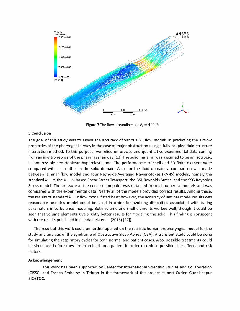
Figure 7 The flow streamlines for 𝑃𝑖 = 400Pa

5 Conclusion

The goal of this study was to assess the accuracy of various 3D flow models in predicting the airflow

properties of the pharyngeal airway in the case of major obstruction using a fully coupled fluid-structure

interaction method. To this purpose, we relied on precise and quantitative experimental data coming

from an in-vitro replica of the pharyngeal airway [13].The solid material was assumed to be an isotropic,

incompressible neo-Hookean hyperelastic one. The performances of shell and 3D finite element were

compared with each other in the solid domain. Also, for the fluid domain, a comparison was made

between laminar flow model and four Reynolds-Averaged Navier-Stokes (RANS) models, namely the

standard 𝑘 − 𝜀, the 𝑘 − 𝜔 based Shear Stress Transport, the BSL Reynolds Stress, and the SSG Reynolds

Stress model. The pressure at the constriction point was obtained from all numerical models and was

compared with the experimental data. Nearly all of the models provided correct results. Among these,

the results of standard 𝑘 − 𝜀 flow model fitted best; however, the accuracy of laminar model results was

reasonable and this model could be used in order for avoiding difficulties associated with tuning

parameters in turbulence modeling. Both volume and shell elements worked well; though it could be

seen that volume elements give slightly better results for modeling the solid. This finding is consistent

with the results published in (Landajuela et al. (2016) [27]).

The result of this work could be further applied on the realistic human oropharyngeal model for the

study and analysis of the Syndrome of Obstructive Sleep Apnea (OSA). A transient study could be done

for simulating the respiratory cycles for both normal and patient cases. Also, possible treatments could

be simulated before they are examined on a patient in order to reduce possible side effects and risk

factors.

Acknowledgement

This work has been supported by Center for International Scientific Studies and Collaboration

(CISSC) and French Embassy in Tehran in the framework of the project Hubert Curien Gundishapur

BIOSTOC.

References

[1] Wang, Y., Liu, Y.., Sun, X., Yu, S., Gao, F., 2009. Numerical analysis of respiratory flow patterns

within human upper airway. Acta Mechanica Solida Sinica 25:737-746.

[2] Mylavarapu, G., Murugappan, S., Mihaescu, M., Kalra, M., Khosla, S., Gutmark, E., 2009. Validation

of computational fluid dynamics methodology used for human upper airway flow simulations.

Journal of Biomechanics 42:1553-1559.

[3] Sung, S.J., Jeong, S. J., Yu, S. Y., Hwang, C. J., Pae, E. K., 2006. Customized three-dimensional

Computational fluid dynamics simulation of the upper airway of obstructive sleep apnea. Angle

Orthodontist 76 (5):791-9.

[4] Nithiarasu, P., Hassan, O., Morgan, K., Weatherill, N. P., Fielder, C., Whittet, H., Ebden, P., Lewis,

K. R., 2008. Steady flow through a realistic human upper airway geometry. International Journal

For Numerical Methods In Fluids 57:631-651

[5] Lucey, A. D., King, A. J. C., Tetlow, G. A., Wang, J., Armstrong, J. J., Leigh, M. S., Paduch, A.,

Walsh, J. H., Sampson, D. D., Eastwood, P.R., Hillman, D. R., 2010. Measurement, reconstruction,

and flow-field computation of the human pharynx with application to sleep apnea. IEEE

Transactions on Biomedical Engineering 57(10):2535-2548.

[6] Fujimoto, J. C., Pitris, C., Boppart, S. A., Brezinski, M. E., 2000. Optical Coherence Tomography:

An emerging technology for biomedical imaging and optical biopsy. Neoplasia 2:9-25.

[7] Zhao, M., Barber, T., Cistulli, P. A., Sutherland, K., Rosengarten, G., 2013. Computational fluid

dynamics for the assessment of upper airway response to oral apliance treatment in obstructive

sleep apnea. Journal of Biomechanics 46:142-150.

[8] Wakayama, T., Suzuki, M., Tanuma, T., 2016. Effect of nasal obstruction on continuous positive

airway pressure treatment: Computational Fluid Dynamics Analyses. PLOS ONE 11(3).

[9] Cisonni, J., Lucey, A. D., Walsh, J. H., King, A. J. C., Elliott, N. S.J., Sampson, D. D., Eastwood, P.R.,

Hillman, D. R., 2013. Effect of the velopharynx on intraluminal pressures in reconstructed

pharynges derived from individuals with and without sleep apnea. Journal of Biomechanics

46(14):2504-2512.

[10] Pelteret, J.-P. V., Reddy, B., 2014. Development of a computational biomechanical model of the

human upper airway soft tissues toward simulating obstructive sleep apnea. Clinical Anatomy

27:182-200.

[11] Carrigy, N. B., Carey, J. P., Martin, A. R., Remmers, J. E., Zaerian, A., Topor, Z., Grosse, Z., Noga,

M., Finlay, W. H., 2015. Simulation of muscle and adipose tissue deformation in the passive

human pharynx. Computer Methods in Biomechanics and Biomedical Engineering 19(7): 1025-

5842.

[12] Huang, Y., Malhotra, A., White, D. P., 2005. Computational simulation of human upper airway

collapse using a pressure-/state-dependent model of genioglossal muscle contraction under

laminar flow conditions. Journal of Applied Physiology 99:1138-1148.

[13] Chouly, F., Van Hirtum, A., Lagree, P.-Y., Pelorson, X., Payan, Y., 2008. Numerical and

experimental study of expiratory flow in the case of major obstructions with fluid-structure

interaction. Journal of Fluids and Structures 24:250-269.

[14] Lagrée, P. Y., Lorthois, S. (2005). The RNS/Prandtl equations and their link with other asymptotic

descriptions: application to the wall shear stress scaling in a constricted pipe. International

Journal of Engineering Science 43(3), 352-378.

[15] Chouly, F., Van Hirtum, A., Lagrée, P. Y., Paoli, J. R., Pelorson, X., & Payan, Y., 2006, Simulation of

the retroglossal fluid-structure interaction during obstructive sleep apnea. Lecture Notes in

Computer Science 4072.

[16] Rasani, M. R., Inthavong, K., Tu, J. Y., 2011. Simulation of pharyngeal airway interaction with

airflow using low-Re turbulence model. Modeling and Simulation in Engineering 510472.

[17] Heil, M., Jensen, O. E., 2003. Flows in deformable tubes and channels. In Flow past highly

compliant boundaries and in collapsible tubes, Springer Netherlands: 15-49.

[18] Wang, Y., Wang, J., Liu, Y., Yu, S., Sun, X., Li, S., Shen, S., Zhao, W. 2012. Fluid–structure

interaction modeling of upper airways before and after nasal surgery for obstructive sleep

apnea. International Journal For Numerical Methods In Biomedical Engineering, 28(5), 528-546.

[19] Zhao, M., Barber, T., Cistulli, P. A., Sutherland, K., Rosengarten, G., 2013. Simulation of upper

airway occlusion without and with mandibular advancement in obstructive sleep apnea. Journal

of Biomechanics 46: 2586-2592.

[20] Kim, S.-H., Chung, S.-K., Na, Y., 2015. Numerical investigation of flow-induced deformation along

the human respiratory upper airway. Journal of Mechanical Science and Technology 29(12):

5267-5272.

[21] Pirnar,J., Dolenc-Groselji, L., Fajdija, I., Zun, I., 2015. Computational fluid-structure interaction

simulation of flow in the human upper airway. Journal of Biomechanics 48: 3685-3691.

[22] Chouly, F., Van Hirtum, A., Lagree, P.-Y., Perloson, X., Payan, Y., 2008. Modelling human

pharyngeal airway: validation of numerical simulations using in vitro experiments. Medical and

Biological Engineering and Computing 47: 49-58.

[23] Nazari, M. A., Perrier, P. , Chabanas, M. , Payan, Y., 2010. Simulation of dynamic orofacial

movements using a constitutive law varying with muscle activation. Computer Methods in

Biomechanics and Biomedical Engineering 13(4): 469-489.

[24] Wilcox, D. C., 1993. Turbulence Modeling for CFD. Glendale, California: DCW Industries, Inc.

[25] Eisfeld, B., 2010. Reynolds stress modelling for complex aerodynamic flows. In European

Conference on Computational Fluid Dynamics, ECCOMAS CFD: 14-17.

[26] Gianopapa, C. G., 2004. Fluid-structure interaction in flexible vessels. PhD thesis, University of

London, King’s College London.

[27] Landajuela, M., Vidrascu, M., Chapelle, D., Fernandez, M. A., 2016. Coupling schemes for FSI

forward prediction challenge: comparative study and validation. International Journal for

Numerical Methods in Biomedical Engineering. In press. DOI:10.1002/cnm.2813.