Component-wise AdaBoost Algorithms forHigh-dimensional Binary Classification and Class

Probability Prediction

Jianghao Chu* Tae-Hwy Lee Aman Ullah

July 31, 2018

Abstract

Freund and Schapire (1997) introduced “Discrete AdaBoost”(DAB) which has beenmysteriously effective for the high-dimensional binary classification or binary predic-tion. In an effort to understand the myth, Friedman, Hastie and Tibshirani (FHT,2000) show that DAB can be understood as statistical learning which builds an addi-tive logistic regression model via Newton-like updating minimization of the“exponentialloss”. From this statistical point of view, FHT proposed three modifications of DAB,namely, Real AdaBoost (RAB), LogitBoost (LB), and Gentle AdaBoost (GAB). All ofDAB, RAB, LB, GAB solve for the logistic regression via different algorithmic designsand different objective functions. The RAB algorithm uses class probability estimatesto construct real-valued contributions of the weak learner, LB is an adaptive Newtonalgorithm by stagewise optimization of the Bernoulli likelihood, and GAB is an adap-tive Newton algorithm via stagewise optimization of the exponential loss. The sameauthors of FHT published an influential textbook, The Elements of Statistical Learn-ing (ESL, 2001 and 2008). A companion book An Introduction to Statistical Learning(ISL) by James et al. (2013) was published with applications in R. However, both ESLand ISL (e.g., sections 4.5 and 4.6) do not cover these four AdaBoost algorithms whileFHT provided some simulation and empirical studies to compare these methods. Givennumerous potential applications, we believe it would be useful to collect the R librariesof these AdaBoost algorithms, as well as more recently developed extensions to Ad-aBoost for probability prediction with examples and illustrations. Therefore, the goalof this chapter is to do just that, i.e., (i) to provide a user guide of these alternativeAdaBoost algorithms with step-by-step tutorial of using R (in a way similar to ISL,e.g., Section 4.6), (ii) to compare AdaBoost with alternative machine learning classifi-cation tools such as the deep neural network (DNN), logistic regression with LASSO

*Department of Economics, University of California, Riverside, 900 University Ave, Riverside, CA 92521,USA. Phone: 951-525-8996, fax: 951-827-5685, e-mail: jianghao.chu@email.ucr.edu.

Department of Economics, University of California, Riverside, 900 University Ave, Riverside, CA 92521,USA. Phone: 951-827-1509, fax: 951-827-5685, e-mail: taelee@ucr.edu.

corresponding author. Department of Economics, University of California, Riverside, 900 UniversityAve, Riverside, CA 92521, USA. Phone: 951-827-1591, fax: 951-827-5685, e-mail: aman.ullah@ucr.edu.

1

and SIM-RODEO, and (iii) to demonstrate the empirical applications in economics,such as prediction of business cycle turning points and directional prediction of stockprice indexes. We revisit Ng (2014) who used DAB for prediction of the business cycleturning points by comparing the results from RAB, LB, GAB, DNN, logistic regressionand SIM-RODEO.

Keywords: AdaBoost, R, Binary classification, Logistic regression, DAB, RAB, LB,GAB, DNN.

1 Introduction

A large number of important variables in economics are binary. Let

π (x) ≡ P (y = 1|x)

and y takes value 1 with probability π (x) and −1 with probability 1−π (x). The studies onmaking the best forecast on y can be classified into two classes (Lahiri and Yang, 2012). Oneis focusing on getting the right probability model π (x), e.g., logit and probit models (Bliss,1934; Cox, 1958; Walker and Duncan, 1967), then making the forecast on y with π (x) > 0.5using the estimated probability model. The other is to get the optimal forecast rule on ydirectly, e.g., the maximum score approach (Manski, 1975, 1985; Elliott and Lieli, 2013),without having to (correctly) model the probability π (x).

Given the availability of high-dimensional data, the binary classification or binary prob-ability prediction problems can be improved by incorporating a large number of covariates(x). A number of new methods are proposed to take advantage of the great number ofcovariates. Freund and Schapire (1997) introduce machine learning method called DiscreteAdaBoost algorithm, which takes a functional descent procedure and selects the covariates(or predictors) sequentially. Friedman et al. (2000) show that AdaBoost can be understoodas a regularized logistic regression, which selects the covariates one-at-a-time. The influentialpaper also discusses several extensions to the original idea of Discrete AdaBoost and pro-poses new Boosting methods, namely Real AdaBoost, LogitBoost and Gentle Boost, whichuses the exponential loss or Bernoulli log-likelihood as fitting criteria. Later on, Friedman(2001) generalize the idea to any fitting criteria and proposes the Gradient Boosting Ma-chine. Buhlmann and Yu (2003) and Buhlmann (2006) propose the L2 Boost and prove itsconsistency for regression and classification. Mease et al. (2007) use the logistic function toconvert the class label output of boosting algorithms into probability and/or quantile predic-tions. Chu et al. (2018a) show the linkage between the Discrete AdaBoost and the maximumscore approach and propose Asymmetric AdaBoost for utility based high-dimensional binaryclassification.

On the other hand, efforts are made to incorporate traditional binary classification andprobability prediction methods into the high-dimensional sparse matrix set-up. The key fea-ture of high-dimensional data is the redundancy of covariates in the data. Hence, methodsare proposed to select useful covariates while/before estimation of the models. Tibshirani(1996) proposes the LASSO that is to add L1 penalty to including more covariates in the

2

model. Zou (2006) drives a necessary condition for consistency of the LASSO variable selec-tion and proposes the Adaptive LASSO which is showed to enjoy oracle property. LASSOtype methods are often used with parametric models such as linear model or logistic model.To relax the parametric assumptions, Lafferty and Wasserman (2008) propose the Regu-larization of the Derivative Expectation Operator (RODEO) for variable selection in kernelregression. Chu et al. (2018b) proposes SIM-RODEO for variable selection in semiparametricsingle-index model. See Su and Zhang (2014) for a thorough review of variable selection innonparametric and semiparametric models.

This paper gives a overview of recently developed machine learning methods, namely Ad-aBoost in the role of binary prediction. AdaBoost algorithm focuses on making the optimalforecast directly without modeling the conditional probability of the events. AdaBoost getsan additive model by iteratively minimizing an exponential loss function. In each iteration,AdaBoost puts more weights on the observations that cannot be predicted correctly usingthe previous predictors. Moreover, AdaBoost algorithm is able to solve classification problemwith high-dimensional data which is an advantage to traditional classification methods.

The rest of the paper is organized as follow. In Section 2 we provide a brief introductionof AdaBoost from minimizing the ‘exponential loss’. In Section 3 we show popular variantsof AdaBoost. Section 5 gives numerical examples of the boosting algorithms. Section 6compares the mentioned boosting algorithms with Deep Neural Network (DNN) and logisticregression with LASSO. Section 7 concludes.

2 AdaBoost

The algorithm of AdaBoost is as shown in Algorithm 1. Let y be the binary class taking avalue in −1, 1 that we wish to predict. Let fm (x) be the weak learner (weak classifier) forthe binary target y that we fit to predict using the high-dimensional covariates x in the mthiteration. Let errm denote the error rate of the weak learner fm (x), and Ew (·) denote theweighted expectation (to be defined below) of the variable in the parenthesis with weight w.Note that the error rate Ew

[1(y 6=fm(x))

]is estimated by errm =

∑ni=1wi1(yi 6=fm(xi)) with the

weight wi given by step 2(c) from the previous iteration. n is the number of observations.The symbol 1(·) is the indicator function which takes the value 1 if a logical condition insidethe parenthesis is satisfied and takes the value 0 otherwise. The symbol sign(z) = 1 if z > 0,sign(z) = −1 if z < 0, and hence sign(z) = 1(z>0) − 1(z<0).

3

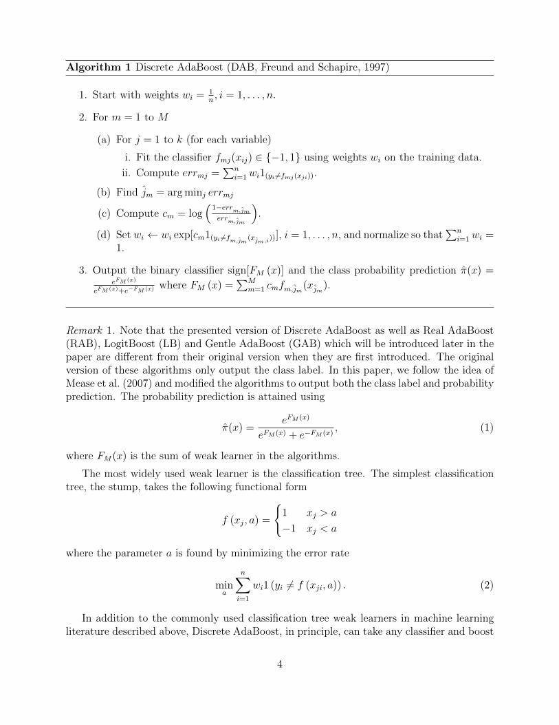
Algorithm 1 Discrete AdaBoost (DAB, Freund and Schapire, 1997)

1. Start with weights wi = 1n, i = 1, . . . , n.

2. For m = 1 to M

(a) For j = 1 to k (for each variable)

i. Fit the classifier fmj(xij) ∈ −1, 1 using weights wi on the training data.

ii. Compute errmj =∑n

i=1wi1(yi 6=fmj(xji)).

(b) Find jm = arg minj errmj

(c) Compute cm = log(

1−errm,jm

errm,jm

).

(d) Set wi ← wi exp[cm1(yi 6=fm,jm(xjm,i))

], i = 1, . . . , n, and normalize so that∑n

i=1wi =1.

3. Output the binary classifier sign[FM (x)] and the class probability prediction π(x) =eFM (x)

eFM (x)+e−FM (x) where FM (x) =∑M

m=1 cmfm,jm(xjm).

Remark 1. Note that the presented version of Discrete AdaBoost as well as Real AdaBoost(RAB), LogitBoost (LB) and Gentle AdaBoost (GAB) which will be introduced later in thepaper are different from their original version when they are first introduced. The originalversion of these algorithms only output the class label. In this paper, we follow the idea ofMease et al. (2007) and modified the algorithms to output both the class label and probabilityprediction. The probability prediction is attained using

π(x) =eFM (x)

eFM (x) + e−FM (x), (1)

where FM(x) is the sum of weak learner in the algorithms.

The most widely used weak learner is the classification tree. The simplest classificationtree, the stump, takes the following functional form

f (xj, a) =

1 xj > a

−1 xj < a

where the parameter a is found by minimizing the error rate

mina

n∑i=1

wi1 (yi 6= f (xji, a)) . (2)

In addition to the commonly used classification tree weak learners in machine learningliterature described above, Discrete AdaBoost, in principle, can take any classifier and boost

4

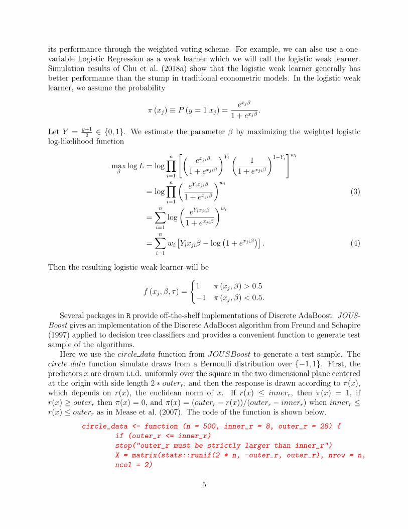
its performance through the weighted voting scheme. For example, we can also use a one-variable Logistic Regression as a weak learner which we will call the logistic weak learner.Simulation results of Chu et al. (2018a) show that the logistic weak learner generally hasbetter performance than the stump in traditional econometric models. In the logistic weaklearner, we assume the probability

π (xj) ≡ P (y = 1|xj) =exjβ

1 + exjβ.

Let Y = y+12∈ 0, 1. We estimate the parameter β by maximizing the weighted logistic

log-likelihood function

maxβ

logL = logn∏i=1

[(exjiβ

1 + exjiβ

)Yi ( 1

1 + exjiβ

)1−Yi]wi

= logn∏i=1

(eYixjiβ

1 + exjiβ

)wi

(3)

=n∑i=1

log

(eYixjiβ

1 + exjiβ

)wi

=n∑i=1

wi[Yixjiβ − log

(1 + exjiβ

)]. (4)

Then the resulting logistic weak learner will be

f (xj, β, τ) =

1 π (xj, β) > 0.5

−1 π (xj, β) < 0.5.

Several packages in R provide off-the-shelf implementations of Discrete AdaBoost. JOUS-Boost gives an implementation of the Discrete AdaBoost algorithm from Freund and Schapire(1997) applied to decision tree classifiers and provides a convenient function to generate testsample of the algorithms.

Here we use the circle data function from JOUSBoost to generate a test sample. Thecircle data function simulate draws from a Bernoulli distribution over −1, 1. First, thepredictors x are drawn i.i.d. uniformly over the square in the two dimensional plane centeredat the origin with side length 2 ∗ outerr, and then the response is drawn according to π(x),which depends on r(x), the euclidean norm of x. If r(x) ≤ innerr, then π(x) = 1, ifr(x) ≥ outerr then π(x) = 0, and π(x) = (outerr − r(x))/(outerr − innerr) when innerr ≤r(x) ≤ outerr as in Mease et al. (2007). The code of the function is shown below.

circle_data <- function (n = 500, inner_r = 8, outer_r = 28)

if (outer_r <= inner_r)

stop("outer_r must be strictly larger than inner_r")

X = matrix(stats::runif(2 * n, -outer_r, outer_r), nrow = n,

ncol = 2)

5

r = apply(X, 1, function(x) sqrt(sum(x^2)))

p = 1 * (r < inner_r) + (outer_r - r)/(outer_r - inner_r) *

((inner_r < r) & (r < outer_r))

y = 2 * stats::rbinom(n, 1, p) - 1

list(X = X, y = y, p = p)

Then we use the implementation of Discrete AdaBoost from ada package since the adapackage provides implementation of not only Discrete AdaBoost and also Real AdaBoost,LogitBoost and Gentle AdaBoost which we will discuss about in the next section.

#Generate data from the circle model

library(JOUSBoost)

set.seed(111)

dat <- circle_data(n = 500)

x <- dat$X

y <- dat$y

library(ada)

model <- ada(x, y, loss = "exponential", type = "discrete", iter = 200)

print(model)

where y and x are the training samples, and iter controls the number of boosting iterations.

Remark 2. The algorithms in ada for Discrete AdaBoost, Real AdaBoost, LogitBoost andGentle Boost may not follow exactly the same steps and/or criteria as described in the paper.However, the major settings, the loss function and characteristics of weak learners, are thesame. We choose to use the ada package since it’s widely accessible and easy to use for thereaders.

The output is as follow.

Call:

ada(x, y = y, loss = "exponential", type = "discrete", iter = 200)

Loss: exponential Method: discrete Iteration: 200

Final Confusion Matrix for Data:

Final Prediction

True value -1 1

-1 300 14

1 15 171

Train Error: 0.058

Out-Of-Bag Error: 0.094 iteration= 195

6

Additional Estimates of number of iterations:

train.err1 train.kap1

197 197

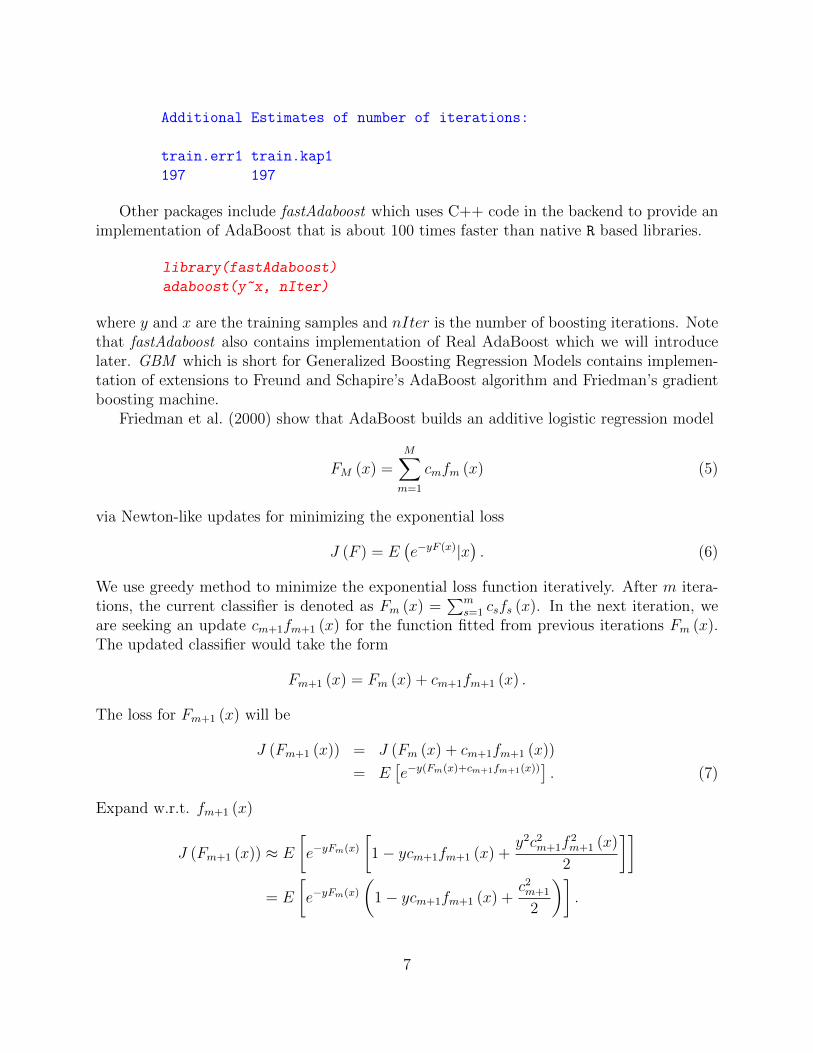
Other packages include fastAdaboost which uses C++ code in the backend to provide animplementation of AdaBoost that is about 100 times faster than native R based libraries.

library(fastAdaboost)

adaboost(y~x, nIter)

where y and x are the training samples and nIter is the number of boosting iterations. Notethat fastAdaboost also contains implementation of Real AdaBoost which we will introducelater. GBM which is short for Generalized Boosting Regression Models contains implemen-tation of extensions to Freund and Schapire’s AdaBoost algorithm and Friedman’s gradientboosting machine.

Friedman et al. (2000) show that AdaBoost builds an additive logistic regression model

FM (x) =M∑m=1

cmfm (x) (5)

via Newton-like updates for minimizing the exponential loss

J (F ) = E(e−yF (x)|x

). (6)

We use greedy method to minimize the exponential loss function iteratively. After m itera-tions, the current classifier is denoted as Fm (x) =

∑ms=1 csfs (x). In the next iteration, we

are seeking an update cm+1fm+1 (x) for the function fitted from previous iterations Fm (x).The updated classifier would take the form

Fm+1 (x) = Fm (x) + cm+1fm+1 (x) .

The loss for Fm+1 (x) will be

J (Fm+1 (x)) = J (Fm (x) + cm+1fm+1 (x))

= E[e−y(Fm(x)+cm+1fm+1(x))

]. (7)

Expand w.r.t. fm+1 (x)

J (Fm+1 (x)) ≈ E

[e−yFm(x)

[1− ycm+1fm+1 (x) +

y2c2m+1f2m+1 (x)

2

]]= E

[e−yFm(x)

(1− ycm+1fm+1 (x) +

c2m+1

2

)].

7

The last equality holds since y ∈ −1, 1 , fm+1 (x) ∈ −1, 1, and y2 = f 2m+1 (x) = 1.

fm+1 (x) only appears in the second term in the parenthesis, so minimizing the loss function(7) w.r.t. fm+1 (x) is equivalent to maximizing the second term in the parenthesis whichresults in the following conditional expectation

maxf

E[e−yFm(x)ycm+1fm+1 (x) |x

].

For any c > 0 (we will prove this later), we can omit cm+1 in the above objective function

maxf

E[e−yFm(x)yfm+1 (x) |x

].

To compare it with the Discrete AdaBoost algorithm, here we define weight w = w (y, x) =e−yFm(x). Later we will see that this weight w is equivalent to that shown in the DiscreteAdaBoost algorithm. So the above optimization can be seen as maximizing a weightedconditional expectation

maxf

Ew [yfm+1 (x) |x] (8)

where Ew (y|x) := E(wy|x)E(w|x) refers to a weighted conditional expectation. Note that (8)

Ew [yfm+1 (x) |x]

= Pw (y = 1|x) fm+1 (x)− Pw (y = −1|x) fm+1 (x)

= [Pw (y = 1|x)− Pw (y = −1|x)] fm+1 (x)

= Ew (y|x) fm+1 (x) .

where Pw (y|x) = E(w|y,x)P (y|x)E(w|x) . Solve the maximization problem (8). Since fm+1 (x) only

takes 1 or -1, it should be positive whenever Ew (y|x) is positive and -1 whenever Ew (y|x)is negative. The solution for fm+1 (x) is

fm+1 (x) =

1 Ew (y|x) > 0

−1 otherwise.

Next, minimize the loss function (7) w.r.t. cm+1

cm+1 = arg mincm+1

Ew(e−cm+1yfm+1(x)

)Ew(e−cm+1yfm+1(x)

)= Pw (y = fm+1 (x)) e−cm+1 + Pw (y 6= fm+1 (x)) ecm+1

∂Ew(e−cyfm+1(x)

)∂c

= −Pw (y = fm+1 (x)) cm+1e−cm+1 + Pw (y 6= fm+1 (x)) cm+1e

cm+1

Let∂Ew

(e−cm+1yfm+1(x)

)∂cm+1

= 0,

8

and we have

Pw (y = fm+1 (x)) cm+1e−cm+1 = Pw (y 6= fm+1 (x)) cm+1e

cm+1 ,

Solve for cm+1, we obtain

cm+1 =1

2log

Pw (y = fm+1 (x))

Pw (y 6= fm+1 (x))=

1

2log

(1− errm+1

errm+1

),

where errm+1 = Pw (y 6= fm+1 (x)) is the error rate of fm+1 (x). Note that cm+1 > 0 as longas the error rate is smaller than 50%. Our assumption cm+1 > 0 holds for any learner thatis better than random guessing.

Now we have finished the steps of one iteration and can get our updated classifier by

Fm+1 (x)← Fm (x) +

(1

2log

(1− errm+1

errm+1

))fm+1 (x) .

Note that in the next iteration, the weight we defined wm+1 will be

wm+1 = e−yFm+1(x) = e−y(Fm(x)+cm+1fm+1(x)) = wm × e−cm+1fm+1(x)y.

Since −yfm+1 (x) = 2× 1y 6=fm+1(x) − 1, the update is equivalent to

wm+1 = wm × e(log

(1−errm+1errm+1

)1[y 6=fm+1(x)]

)= wm ×

(1− errm+1

errm+1

)1[y 6=fm+1(x)]

.

Thus the function and weights update are of an identical form to those used in AdaBoost.AdaBoost could do better than any single weak classifier since it iteratively minimizes theloss function via a Newton-like procedure. Interestingly, the function F (x) from minimizingthe exponential loss is the same as maximizing a logistic log-likelihood. Let

J (F (x)) = E[E(e−yF (x)|x

)]= E

[P (y = 1|x) e−F (x) + P (y = −1|x) eF (x)

].

Taking derivative w.r.t. F (x) and making it equal to zero, we obtain

∂E(e−yF (x)|x

)∂F (x)

= −P (y = 1|x) e−F (x) + P (y = −1|x) eF (x) = 0

F ∗ (x) =1

2log

[P (y = 1|x)

P (y = −1|x)

].

Moreover, if the true probability

P (y = 1|x) =e2F (x)

1 + e2F (x),

9

for Y = y+12

, the log-likelihood is

E (logL|x) = E[2Y F (x)− log

(1 + e2F (x)

)|x].

The solution F ∗ (x) that maximize the log-likelihood must equals the F (x) in the true model

P (y = 1|x) = e2F (x)

1+e2F (x) . Hence,

e2F∗(x) = P (y = 1|x)

(1 + e2F

∗(x))

e2F∗(x) =

P (y = 1|x)

1− P (y = 1|x)

F ∗ (x) =1

2log

[P (y = 1|x)

P (y = −1|x)

]. (9)

AdaBoost that minimizes the exponential loss yield the same solution as logistic regressionthat maximizes the logistic log-likelihood.

3 Extensions to AdaBoost Algorithms

In this section we introduce extensions of Discrete AdaBoost, namely Real AdaBoost (RAB),LogitBoost (LB) and Gentle AdaBoost (GAB), and discuss how some aspects of the DABmay be modified to yield RAB, LB and GAB. In the last section, we learned that DiscreteAdaBoost minimizes an exponential loss via iteratively adding a binary weaker learner tothe pool of weak learners. The addition of a new weak learner can be seen as taking a stepon the direction that loss function descents in the Newton method. There are two majorways to extend the idea of Discrete AdaBoost. One focuses on making the minimizationmethod more efficient by adding a more flexible weak learner. The other is to use differentloss functions that may lead to better results. Next, we give an introduction to severalextensions of Discrete AdaBoost.

10

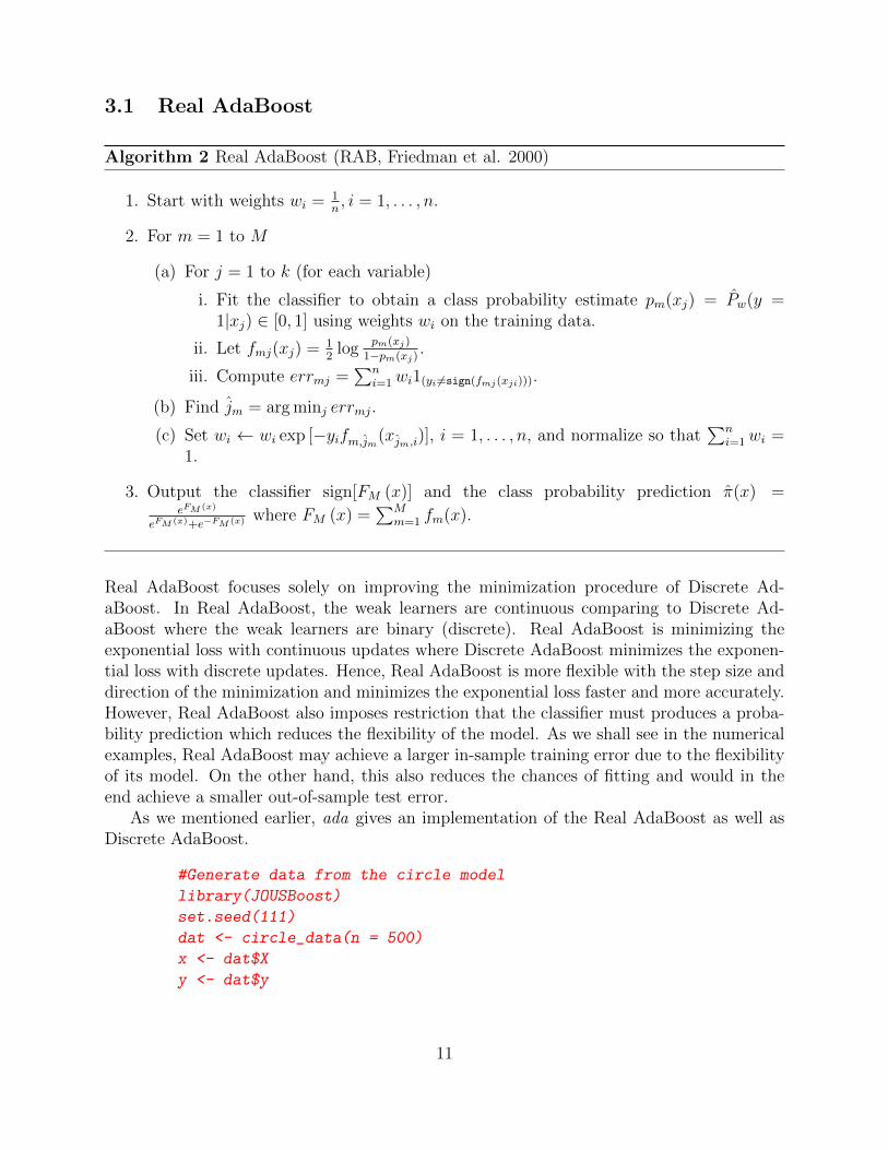
3.1 Real AdaBoost

Algorithm 2 Real AdaBoost (RAB, Friedman et al. 2000)

1. Start with weights wi = 1n, i = 1, . . . , n.

2. For m = 1 to M

(a) For j = 1 to k (for each variable)

i. Fit the classifier to obtain a class probability estimate pm(xj) = Pw(y =1|xj) ∈ [0, 1] using weights wi on the training data.

ii. Let fmj(xj) = 12

logpm(xj)

1−pm(xj).

iii. Compute errmj =∑n

i=1wi1(yi 6=sign(fmj(xji))).

(b) Find jm = arg minj errmj.

(c) Set wi ← wi exp [−yifm,jm(xjm,i)], i = 1, . . . , n, and normalize so that∑n

i=1wi =1.

3. Output the classifier sign[FM (x)] and the class probability prediction π(x) =eFM (x)

eFM (x)+e−FM (x) where FM (x) =∑M

m=1 fm(x).

Real AdaBoost focuses solely on improving the minimization procedure of Discrete Ad-aBoost. In Real AdaBoost, the weak learners are continuous comparing to Discrete Ad-aBoost where the weak learners are binary (discrete). Real AdaBoost is minimizing theexponential loss with continuous updates where Discrete AdaBoost minimizes the exponen-tial loss with discrete updates. Hence, Real AdaBoost is more flexible with the step size anddirection of the minimization and minimizes the exponential loss faster and more accurately.However, Real AdaBoost also imposes restriction that the classifier must produces a proba-bility prediction which reduces the flexibility of the model. As we shall see in the numericalexamples, Real AdaBoost may achieve a larger in-sample training error due to the flexibilityof its model. On the other hand, this also reduces the chances of fitting and would in theend achieve a smaller out-of-sample test error.

As we mentioned earlier, ada gives an implementation of the Real AdaBoost as well asDiscrete AdaBoost.

#Generate data from the circle model

library(JOUSBoost)

set.seed(111)

dat <- circle_data(n = 500)

x <- dat$X

y <- dat$y

11

library(ada)

model <- ada(x, y, loss = "exponential", type = "real", iter = 200)

print(model)

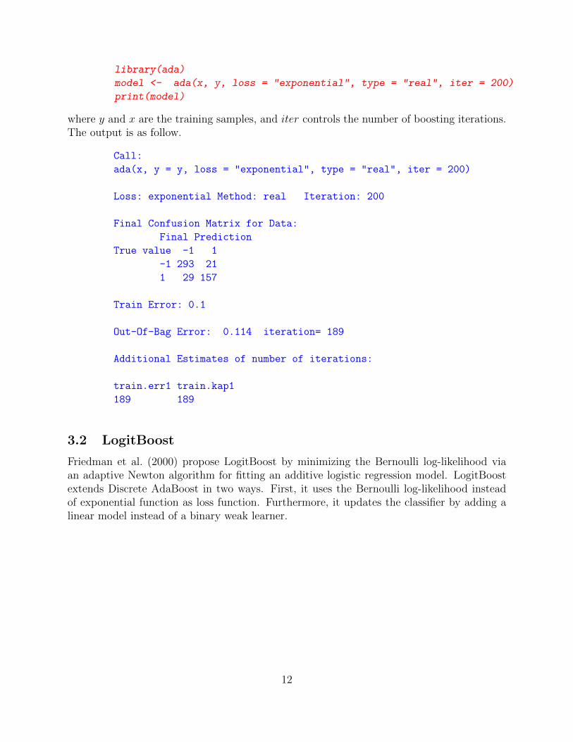
where y and x are the training samples, and iter controls the number of boosting iterations.The output is as follow.

Call:

ada(x, y = y, loss = "exponential", type = "real", iter = 200)

Loss: exponential Method: real Iteration: 200

Final Confusion Matrix for Data:

Final Prediction

True value -1 1

-1 293 21

1 29 157

Train Error: 0.1

Out-Of-Bag Error: 0.114 iteration= 189

Additional Estimates of number of iterations:

train.err1 train.kap1

189 189

3.2 LogitBoost

Friedman et al. (2000) propose LogitBoost by minimizing the Bernoulli log-likelihood viaan adaptive Newton algorithm for fitting an additive logistic regression model. LogitBoostextends Discrete AdaBoost in two ways. First, it uses the Bernoulli log-likelihood insteadof exponential function as loss function. Furthermore, it updates the classifier by adding alinear model instead of a binary weak learner.

12

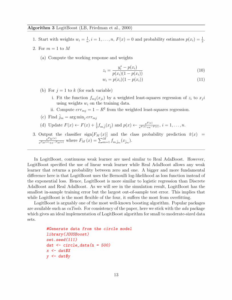
Algorithm 3 LogitBoost (LB, Friedman et al., 2000)

1. Start with weights wi = 1n, i = 1, . . . , n, F (x) = 0 and probability estimates p(xi) = 1

2.

2. For m = 1 to M

(a) Compute the working response and weights

zi =y∗i − p(xi)

p(xi)(1− p(xi))(10)

wi = p(xi)(1− p(xi)) (11)

(b) For j = 1 to k (for each variable)

i. Fit the function fmj(xji) by a weighted least-squares regression of zi to xjiusing weights wi on the training data.

ii. Compute errmj = 1−R2 from the weighted least-squares regression.

(c) Find jm = arg minj errmj

(d) Update F (x)← F (x) + 12fm,j(xj) and p(x)← eF (x)

eF (x)+e−F (x) , i = 1, . . . , n.

3. Output the classifier sign[FM (x)] and the class probability prediction π(x) =eFM (x)

eFM (x)+e−FM (x) where FM (x) =∑M

m=1 fm,jm(xjm).

In LogitBoost, continuous weak learner are used similar to Real AdaBoost. However,LogitBoost specified the use of linear weak learner while Real AdaBoost allows any weaklearner that returns a probability between zero and one. A bigger and more fundamentaldifference here is that LogitBoost uses the Bernoulli log-likelihood as loss function instead ofthe exponential loss. Hence, LogitBoost is more similar to logistic regression than DiscreteAdaBoost and Real AdaBoost. As we will see in the simulation result, LogitBoost has thesmallest in-sample training error but the largest out-of-sample test error. This implies thatwhile LogitBoost is the most flexible of the four, it suffers the most from overfitting.

LogitBoost is arguably one of the most well-known boosting algorithm. Popular packagesare available such as caTools. For consistency of the paper, here we stick with the ada packagewhich gives an ideal implementation of LogitBoost algorithm for small to moderate-sized datasets.

#Generate data from the circle model

library(JOUSBoost)

set.seed(111)

dat <- circle_data(n = 500)

x <- dat$X

y <- dat$y

13

library(ada)

model <- ada(x, y, loss = "logistic", type = "gentle", iter = 200)

print(model)

where y and x are the training samples, and iter controls the number of boosting iterations.The output is as follow.

Call:

ada(x, y = y, loss = "logisitc", type = "gentle", iter = 200)

Loss: logisitc Method: gentle Iteration: 200

Final Confusion Matrix for Data:

Final Prediction

True value -1 1

-1 309 5

1 8 178

Train Error: 0.026

Out-Of-Bag Error: 0.07 iteration= 196

Additional Estimates of number of iterations:

train.err1 train.kap1

195 195

14

3.3 Gentle AdaBoost

Algorithm 4 Gentle AdaBoost (GAB, Friedman et al. 2010)

1. Start with weights wi = 1n, i = 1, . . . , n.

2. For m = 1 to M

(a) For j = 1 to k (for each variable)

i. Fit the regression function fmj(xij) by weighted least-squares of yi on xi usingweights wi on the training data.

ii. Compute errmj = 1−R2 from the weighted least-squares regression.

(b) Find jm = arg minj errmj

(c) Set wi ← wi exp[−yifm,jm(xjm,i)], i = 1, . . . , n, and normalize so that∑n

i=1wi = 1.

3. Output the classifier sign[FM (x)] and the class probability prediction π(x) =eFM (x)

eFM (x)+e−FM (x) where FM (x) =∑M

m=1 fm,jm(xjm).

Gentle AdaBoost extends Discrete AdaBoost in the sense that it allows each weak learner tobe a linear model. This is similar to LogitBoost and more flexible than Discrete AdaBoostand Real AdaBoost. However, it is closer to Discrete AdaBoost and Real AdaBoost thanLogitBoost in the sense that Gentle AdaBoost, Discrete AdaBoost and Real AdaBoost allminimize the exponential loss while LogitBoost minimizes the Bernoulli log-likelihood. An-other point that Gentle AdaBoost is more similar to Real AdaBoost than Discrete AdaBoostis that since the weak learners are continuous, there is no need to find an optimal step size foreach iteration because the weak learner is already optimal. As we will see in the simulationresults, Gentle Boost often lies between Real AdaBoost and LogitBoost in terms of in-sampletraining error and out-of-sample test error.

ada also gives an implementation of the Gentle AdaBoost algorithm.

#Generate data from the circle model

library(JOUSBoost)

set.seed(111)

dat <- circle_data(n = 500)

x <- dat$X

y <- dat$y

library(ada)

model <- ada(x, y, loss = "exponential", type = "gentle", iter = 200)

print(model)

where y and x are the training samples, and iter controls the number of boosting iterations.The output is as follow.

15

Call:

ada(x, y = y, loss = "exponential", type = "gentle", iter = 200)

Loss: exponential Method: gentle Iteration: 200

Final Confusion Matrix for Data:

Final Prediction

True value -1 1

-1 305 9

1 15 171

Train Error: 0.048

Out-Of-Bag Error: 0.078 iteration= 198

Additional Estimates of number of iterations:

train.err1 train.kap1

196 196

For all the four boosting algorithms mentioned above, ada outputs the class label bydefault. However, we can use the command predict to output probability prediction and/orof class label using ada.

#Generate data from the circle model

library(JOUSBoost)

set.seed(111)

dat <- circle_data(n = 500)

x <- dat$X

y <- dat$y

library(ada)

model <- ada(x, y, loss = "exponential", type = "discrete", iter = 200)

#New Data for Prediction

newx <- data.frame(1,1)

names(newx) <- c('V1', 'V2')

predict(model, newdata = newx, type = "F")

predict(model, newdata = newx, type = "prob")

where y and x are the training samples, iter controls the number of boosting iterations. modelis the output from fitting the model using ada, newdata is the data to be used in predictionand type specifies the type of output from the predict function. When type = “vector”, thefunction outputs class labels. When type = “F”, the function outputs F (x) which the sumof all weak learners. When type = “prob”, the function outputs the class probability using1. The output is as follow.

16

> predict(model, newdata = newx, type = "F")

1

4.345358

> predict(model, newdata = newx, type = "prob")

[,1] [,2]

1 0.0001681114 0.9998319

Note that manually transforming the sum of all weak learners F (x) into probability predictionusing equation 9 would lead to the same result as directly output the probability predictionfrom the package as in the second line.

4 Alternative Classification Methods

Apart from Boosting algorithms, we also consider Deep Neural Network, Logistic Regres-sion and semiparametric single-index model as alternative methods to obtain a predictorof y. Deep Neural Network is able to deal with high-dimensional data. For Logistic Re-gression, we have to select useful information from noises. Hence, a shrinkage parameteris used with the logistic log-likelihood which we call LASSO. Semiparametric single-indexmodel is an extension to parametric single-index model such as Logistic Regression. It re-laxes the parametric assumptions and uses the kernel function of fit the data locally. Forhigh-dimensional problem, we use SIM-RODEO to select useful explanation variables forsemiparametric single-index models.

4.1 Deep Neural Network

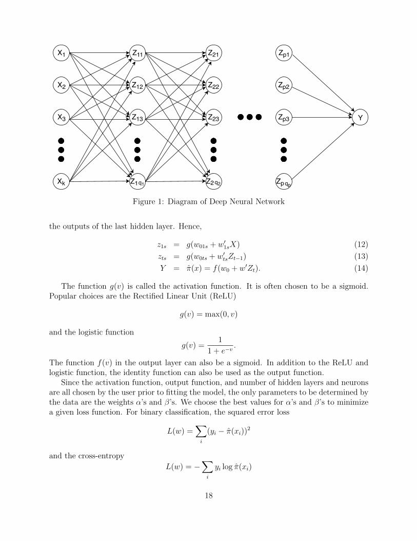
Deep Neural Network is undoubtedly one of the most state-of-the-art classification methods.The model is similar to a multi-stage regression or classification model. The idea is to builda flexible nonlinear statistical model consisted of several layers and each layer is consisted ofneurons as in Figure 1.

For binary classification, there is only one output Y that is the class probability or classlabel. Since the transformation from class probability to class label is straight-forward, wefocus on the case where the output is the class probability. The layer labeled X is theinput layer which contains all the explanatory variables in the data set. Note that thenumber of explanatory variables k is allowed to be extremely large (larger than the numberof observations) as in high-dimensional settings. The layers labeled Z are the hidden layers.The number of hidden layers p can be arbitrarily set by the user and each hidden layer cancontain arbitrarily many neurons denoted by qt where t stands for the tth hidden layer.

The output zts of the sth neuron in the tth hidden layer is normally a single-index functiong(αts+β

′tsZt−1) where α is a scalar, β is a vector of same length qt−1 as the number of neurons

in the (t−1)th hidden layer or the input layer if t = 1 and Zt−1 = (zt−1,1, zt−1,2, . . . , zt−1,qt−1)is a vector of outputs from all neurons of the (t − 1)th hidden layer or the input layer ift = 1. Similarly, the output layer of the model is also chosen to be a single-index function of

17

X1

X2

X3

Xk

Z11

Z12

Z13

Z1q1

Zp1

Zp2

Zp3

Zpqp

Y

Z21

Z22

Z23

Z2q2

Figure 1: Diagram of Deep Neural Network

the outputs of the last hidden layer. Hence,

z1s = g(w01s + w′1sX) (12)

zts = g(w0ts + w′tsZt−1) (13)

Y = π(x) = f(w0 + w′Zt). (14)

The function g(v) is called the activation function. It is often chosen to be a sigmoid.Popular choices are the Rectified Linear Unit (ReLU)

g(v) = max(0, v)

and the logistic function

g(v) =1

1 + e−v.

The function f(v) in the output layer can also be a sigmoid. In addition to the ReLU andlogistic function, the identity function can also be used as the output function.

Since the activation function, output function, and number of hidden layers and neuronsare all chosen by the user prior to fitting the model, the only parameters to be determined bythe data are the weights α’s and β’s. We choose the best values for α’s and β’s to minimizea given loss function. For binary classification, the squared error loss

L(w) =∑i

(yi − π(xi))2

and the cross-entropy

L(w) = −∑i

yi log π(xi)

18

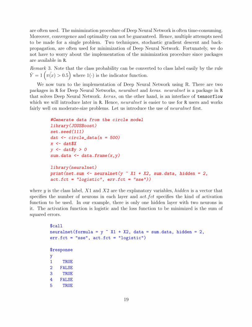
are often used. The minimization procedure of Deep Neural Network is often time-consuming.Moreover, convergence and optimality can not be guaranteed. Hence, multiple attempts needto be made for a single problem. Two techniques, stochastic gradient descent and back-propagation, are often used for minimization of Deep Neural Network. Fortunately, we donot have to worry about the implementation of the minimization procedure since packagesare available in R.

Remark 3. Note that the class probability can be converted to class label easily by the rule

Y = 1(

ˆπ(x) > 0.5)

where 1(·) is the indicator function.

We now turn to the implementation of Deep Neural Network using R. There are twopackages in R for Deep Neural Networks, neuralnet and keras. neuralnet is a package in R

that solves Deep Neural Network. keras, on the other hand, is an interface of tensorflow

which we will introduce later in R. Hence, neuralnet is easier to use for R users and worksfairly well on moderate-size problems. Let us introduce the use of neuralnet first.

#Generate data from the circle model

library(JOUSBoost)

set.seed(111)

dat <- circle_data(n = 500)

x <- dat$X

y <- dat$y > 0

sum.data <- data.frame(x,y)

library(neuralnet)

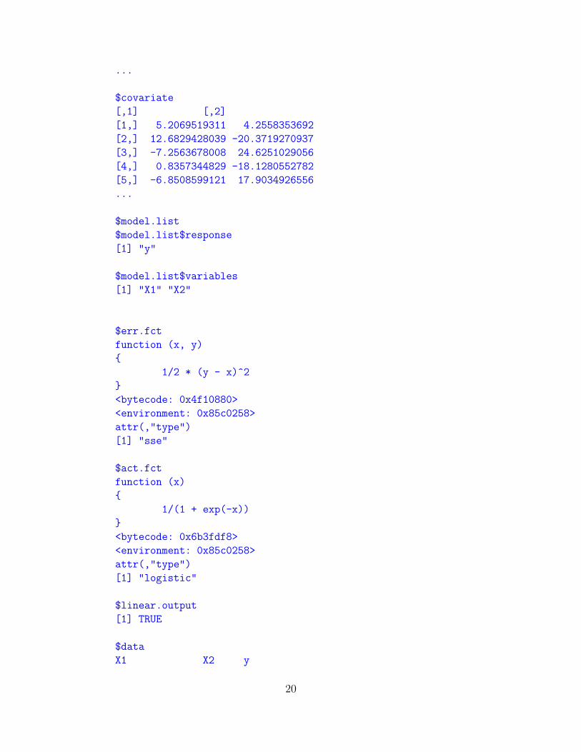
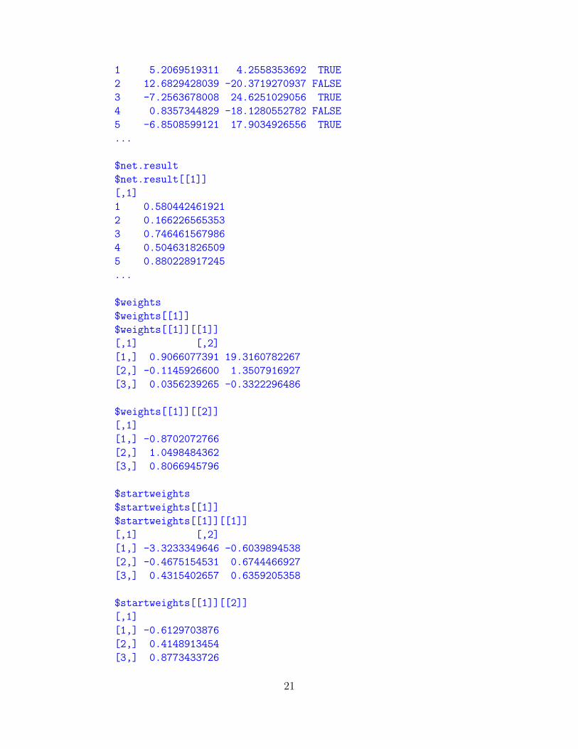
print(net.sum <- neuralnet(y ~ X1 + X2, sum.data, hidden = 2,

act.fct = "logistic", err.fct = "sse"))

where y is the class label, X1 and X2 are the explanatory variables, hidden is a vector thatspecifies the number of neurons in each layer and act.fct specifies the kind of activationfunction to be used. In our example, there is only one hidden layer with two neurons init. The activation function is logistic and the loss function to be minimized is the sum ofsquared errors.

$call

neuralnet(formula = y ~ X1 + X2, data = sum.data, hidden = 2,

err.fct = "sse", act.fct = "logistic")

$response

y

1 TRUE

2 FALSE

3 TRUE

4 FALSE

5 TRUE

19

...

$covariate

[,1] [,2]

[1,] 5.2069519311 4.2558353692

[2,] 12.6829428039 -20.3719270937

[3,] -7.2563678008 24.6251029056

[4,] 0.8357344829 -18.1280552782

[5,] -6.8508599121 17.9034926556

...

$model.list

$model.list$response

[1] "y"

$model.list$variables

[1] "X1" "X2"

$err.fct

function (x, y)

1/2 * (y - x)^2

<bytecode: 0x4f10880>

<environment: 0x85c0258>

attr(,"type")

[1] "sse"

$act.fct

function (x)

1/(1 + exp(-x))

<bytecode: 0x6b3fdf8>

<environment: 0x85c0258>

attr(,"type")

[1] "logistic"

$linear.output

[1] TRUE

$data

X1 X2 y

20

1 5.2069519311 4.2558353692 TRUE

2 12.6829428039 -20.3719270937 FALSE

3 -7.2563678008 24.6251029056 TRUE

4 0.8357344829 -18.1280552782 FALSE

5 -6.8508599121 17.9034926556 TRUE

...

$net.result

$net.result[[1]]

[,1]

1 0.580442461921

2 0.166226565353

3 0.746461567986

4 0.504631826509

5 0.880228917245

...

$weights

$weights[[1]]

$weights[[1]][[1]]

[,1] [,2]

[1,] 0.9066077391 19.3160782267

[2,] -0.1145926600 1.3507916927

[3,] 0.0356239265 -0.3322296486

$weights[[1]][[2]]

[,1]

[1,] -0.8702072766

[2,] 1.0498484362

[3,] 0.8066945796

$startweights

$startweights[[1]]

$startweights[[1]][[1]]

[,1] [,2]

[1,] -3.3233349646 -0.6039894538

[2,] -0.4675154531 0.6744466927

[3,] 0.4315402657 0.6359205358

$startweights[[1]][[2]]

[,1]

[1,] -0.6129703876

[2,] 0.4148913454

[3,] 0.8773433726

21

$generalized.weights

$generalized.weights[[1]]

[,1] [,2]

1 -0.117151263217 0.036419330807

2 -0.148384521998 0.046128951957

3 0.910325193217 -0.221275093627

4 -0.119499601088 0.037149368973

5 0.071284648051 -0.011543348159

...

$result.matrix

1

error 8.553736459613

reached.threshold 0.009821180033

steps 2145.000000000000

Intercept.to.1layhid1 0.906607739056

X1.to.1layhid1 -0.114592659965

X2.to.1layhid1 0.035623926505

Intercept.to.1layhid2 19.316078226658

X1.to.1layhid2 1.350791692688

X2.to.1layhid2 -0.332229648639

Intercept.to.y -0.870207276552

1layhid.1.to.y 1.049848436176

1layhid.2.to.y 0.806694579605

attr(,"class")

[1] "nn"

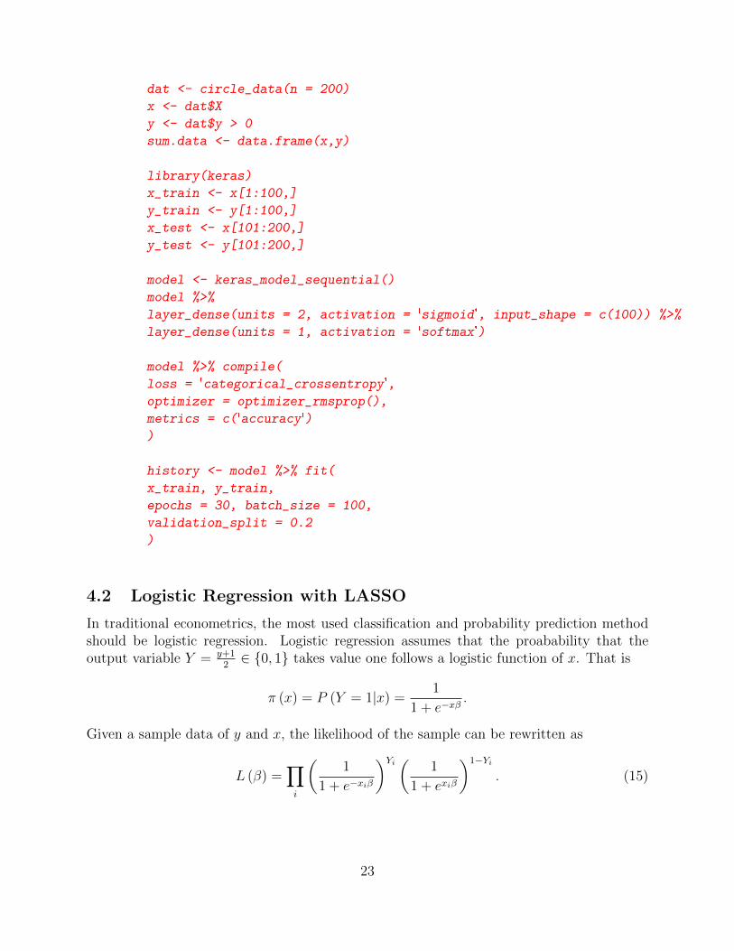
where ... represents that the rest of the output for this feature is omitted.The keras package is a high-level interface of tensorflow which is an open source ma-

chine learning framework maintained by Google and is the most used library for fitting DeepNeural Networks. keras defines the structure and features of the neural network and sendthe informations to tensorflow which then solves the minimization problem and returnsthe results. keras is suitable for more complicated and larger problems since tensorflow

actually doing the hard work.Now we give a simple illustration of constructing neural networks with keras by con-

structing the same network as in the previous example in keras. More details about kerascan be found at https://tensorflow.rstudio.com.

#Generate data from the circle model

library(JOUSBoost)

set.seed(111)

22

dat <- circle_data(n = 200)

x <- dat$X

y <- dat$y > 0

sum.data <- data.frame(x,y)

library(keras)

x_train <- x[1:100,]

y_train <- y[1:100,]

x_test <- x[101:200,]

y_test <- y[101:200,]

model <- keras_model_sequential()

model %>%

layer_dense(units = 2, activation = 'sigmoid', input_shape = c(100)) %>%

layer_dense(units = 1, activation = 'softmax')

model %>% compile(

loss = 'categorical_crossentropy',

optimizer = optimizer_rmsprop(),

metrics = c('accuracy')

)

history <- model %>% fit(

x_train, y_train,

epochs = 30, batch_size = 100,

validation_split = 0.2

)

4.2 Logistic Regression with LASSO

In traditional econometrics, the most used classification and probability prediction methodshould be logistic regression. Logistic regression assumes that the proabability that theoutput variable Y = y+1

2∈ 0, 1 takes value one follows a logistic function of x. That is

π (x) = P (Y = 1|x) =1

1 + e−xβ.

Given a sample data of y and x, the likelihood of the sample can be rewritten as

L (β) =∏i

(1

1 + e−xiβ

)Yi ( 1

1 + exiβ

)1−Yi. (15)

23

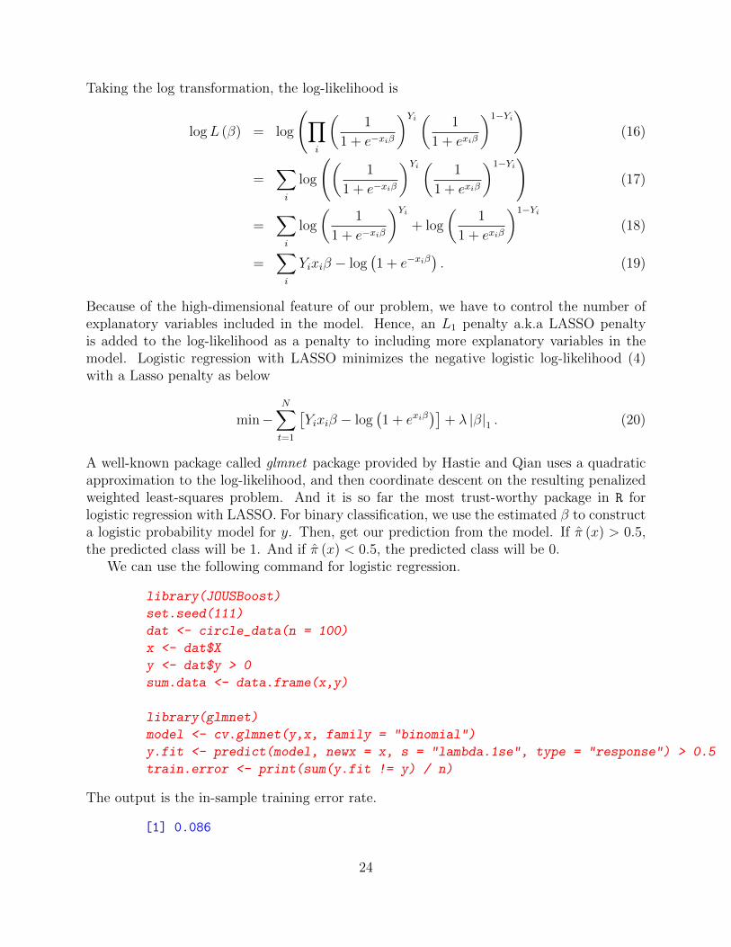
Taking the log transformation, the log-likelihood is

logL (β) = log

(∏i

(1

1 + e−xiβ

)Yi ( 1

1 + exiβ

)1−Yi)

(16)

=∑i

log

((1

1 + e−xiβ

)Yi ( 1

1 + exiβ

)1−Yi)

(17)

=∑i

log

(1

1 + e−xiβ

)Yi+ log

(1

1 + exiβ

)1−Yi(18)

=∑i

Yixiβ − log(1 + e−xiβ

). (19)

Because of the high-dimensional feature of our problem, we have to control the number ofexplanatory variables included in the model. Hence, an L1 penalty a.k.a LASSO penaltyis added to the log-likelihood as a penalty to including more explanatory variables in themodel. Logistic regression with LASSO minimizes the negative logistic log-likelihood (4)with a Lasso penalty as below

min−N∑t=1

[Yixiβ − log

(1 + exiβ

)]+ λ |β|1 . (20)

A well-known package called glmnet package provided by Hastie and Qian uses a quadraticapproximation to the log-likelihood, and then coordinate descent on the resulting penalizedweighted least-squares problem. And it is so far the most trust-worthy package in R forlogistic regression with LASSO. For binary classification, we use the estimated β to constructa logistic probability model for y. Then, get our prediction from the model. If π (x) > 0.5,the predicted class will be 1. And if π (x) < 0.5, the predicted class will be 0.

We can use the following command for logistic regression.

library(JOUSBoost)

set.seed(111)

dat <- circle_data(n = 100)

x <- dat$X

y <- dat$y > 0

sum.data <- data.frame(x,y)

library(glmnet)

model <- cv.glmnet(y,x, family = "binomial")

y.fit <- predict(model, newx = x, s = "lambda.1se", type = "response") > 0.5

train.error <- print(sum(y.fit != y) / n)

The output is the in-sample training error rate.

[1] 0.086

24

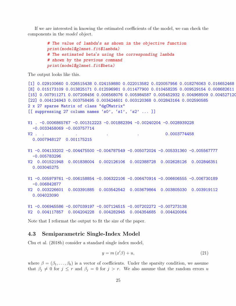
If we are interested in knowing the estimated coefficients of the model, we can check thecomponents in the model object.

# The value of lambda's as shown in the objective function

print(model$glmnet.fit$lambda)

# The estimated beta's using the corresponding lambda

# shown by the previous command

print(model$glmnet.fit$beta)

The output looks like this.

[1] 0.029100660 0.026515438 0.024159880 0.022013582 0.020057956 0.018276063 0.016652468

[8] 0.015173109 0.013825171 0.012596981 0.011477900 0.010458235 0.009529154 0.008682611

[15] 0.007911271 0.007208456 0.006568076 0.005984587 0.005452932 0.004968509 0.004527120

[22] 0.004124943 0.003758495 0.003424601 0.003120368 0.002843164 0.002590585

2 x 27 sparse Matrix of class "dgCMatrix"

[[ suppressing 27 column names ‘s0’, ‘s1’, ‘s2’ ... ]]

V1 . -0.0006865767 -0.001312223 -0.001882394 -0.00240204 -0.0028939228

-0.0033458069 -0.003757714

V2 . . . . . 0.0003774458

0.0007948127 0.001175215

V1 -0.004133202 -0.004475500 -0.004787549 -0.005072024 -0.005331360 -0.005567777

-0.005783296

V2 0.001521948 0.001838004 0.002126106 0.002388728 0.002628126 0.002846351

0.003045275

V1 -0.005979761 -0.006158854 -0.006322106 -0.006470914 -0.006606555 -0.006730189

-0.006842877

V2 0.003226601 0.003391885 0.003542542 0.003679864 0.003805030 0.003919112

0.004023090

V1 -0.006945586 -0.007039197 -0.007124515 -0.007202272 -0.007273138

V2 0.004117857 0.004204228 0.004282945 0.004354685 0.004420064

Note that I reformat the output to fit the size of the paper.

4.3 Semiparametric Single-Index Model

Chu et al. (2018b) consider a standard single index model,

y = m (x′β) + u, (21)

where β = (β1, . . . , βk) is a vector of coefficients. Under the sparsity condition, we assumethat βj 6= 0 for j ≤ r and βj = 0 for j > r. We also assume that the random errors u

25

are independent. However, we allow the presence of heteroskedasticity to encompass a largecategory of models for binary prediction, e.g. Logit and Probit models. The kernel estimator(Ichimura 1993) we use is as shown below

m (x′β;h) =

∑ni=1 yiK

(X′iβ−x′β

h

)∑n

i=1K(X′iβ−x′β

h

) , (22)

where K (·) is a kernel function. The semiparametric kernel regression looks for the bestβ and h to minimize a weighted squared error loss. However, exact identification is notavailable. If one blows up β and θ simultaneously by multiplying the same constant, thekernel estimator would yield identical estimates and losses. The standard identificationapproach is to set the first element of β to be 1 (Ichimura 1993).

In terms of variable selection and prediction, we only need to focus on finding the bestθ ≡ β

h. Hence, we can simplify the estimator to

m (x′θ) =

∑ni=1 yiK (X ′iθ − x′θ)∑ni=1K (X ′iθ − x′θ)

. (23)

The basic idea of the SIM-Rodeo is to view the local bandwidth selection as a variableselection in sparse semiparametric single index model. The SIM-Rodeo algorithm ampli-fies the inverse of the bandwidths for relevant variables while keeping the inverse of thebandwidths of irrelevant variables relatively small. The SIM-Rodeo algorithm is greedy as itsolves for the locally optimal path choice at each iteration. It can also be shown to attain theconsistency in mean square error when it is applied for sparse semiparametric single indexmodels. SIM-Rodeo is able to distinguish truly relevant explanatory variables from noisyirrelevant variables and gives a consistent estimator of the regression function. In addition,the algorithm is fast to finish the greedy steps.

Now we derive the Rodeo for Single Index Models. First we introduce some notation.Let

Wx =

K (X ′1θ − x′θ) · · · 0...

. . ....

0 · · · K (X ′nθ − x′θ)

(24)

where K (·) is the Gaussian kernel. The standard Ichimura (1993) estimator takes the form

m (x′θ) =

∑ni=1 yiK (X ′iθ − x′θ)∑ni=1K (X ′iθ − x′θ)

= (ι′Wxι)−1ι′Wxy. (25)

26

The derivative of the estimator Zj with respect to θj is

Zj ≡∂m (x′θ)

∂θj(26)

= (ι′Wxι)−1ι′∂Wx

∂θjy − (ι′Wxι)

−1ι′∂Wx

∂θjι (ι′Wxι)

−1ι′Wxy

= (ι′Wxι)−1ι′∂Wx

∂θj(y − ιm (x′θ)) . (27)

For the ease of computation, let

Lj =

∂ logK(X′1θ−x′θ)

∂θj· · · 0

.... . .

...

0 · · · ∂ logK(X′nθ−x′θ)∂θj

. (28)

Note that∂Wx

∂θj= WxLj, (29)

which appears in equation (27). With the Gaussian kernel, K (t) = e−t2

2 , then Lj becomes

Lj =

−1

2

∂(X′1θ−x′θ)2

∂θj· · · 0

.... . .

...

0 · · · −12∂(X′nθ−x′θ)

2

∂θj

=

− (X ′1θ − x′θ) (X1j − xj) · · · 0...

. . ....

0 · · · − (X ′nθ − x′θ) (Xnj − xj)

,

where X1j and Xnj are the jth elements of vectors X1 and Xn. And xj is the jth element ofvector x. To simplify the notation, let Bx = (ι′Wxι)

−1 ι′Wx. Then, the derivative Zj becomes

Zj = (ι′Wxι)−1ι′∂Wx

∂θj(y − ιm (x′θ))

= BxLj (I − ιBx) y

≡ Gj (x, θ) y. (30)

Next, we give the conditional expectation and variance of Zj.

Zj = Gj (x, θ) y = Gj (x, θ) (m (x′β) + u) , (31)

E (Zj|X) = E (Gj (x, θ) (m (x′β) + u) |X) = Gj (x, θ)m (x′β) , (32)

Var (Zj|X) = Var (Gj (x, θ) (m (x′β) + u) |X) = σ′Gj (x, θ)′Gj (x, θ)σ, (33)

27

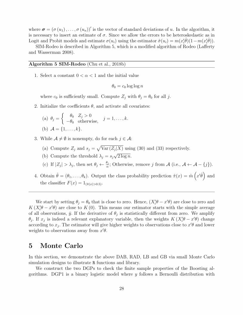
where σ = (σ (u1) , . . . , σ (un))′ is the vector of standard deviations of u. In the algorithm, itis necessary to insert an estimate of σ. Since we allow the errors to be heteroskedastic as inLogit and Probit models and estimate σ(ui) using the estimator σ(ui) = m(x′iθ)(1−m(x′iθ)).

SIM-Rodeo is described in Algorithm 5, which is a modified algorithm of Rodeo (Laffertyand Wasserman 2008).

Algorithm 5 SIM-Rodeo (Chu et al., 2018b)

1. Select a constant 0 < α < 1 and the initial value

θ0 = c0 log log n

where c0 is sufficiently small. Compute Zj with θj = θ0 for all j.

2. Initialize the coefficients θ, and activate all covariates:

(a) θj =

θ0 Zj > 0−θ0 otherwise,

j = 1, . . . , k.

(b) A = 1, . . . , k.

3. While A 6= ∅ is nonempty, do for each j ∈ A:

(a) Compute Zj and sj =√

Var (Zj|X) using (30) and (33) respectively.

(b) Compute the threshold λj = sj√

2 log n.

(c) If |Zj| > λj, then set θj ← θjα

; Otherwise, remove j from A (i.e., A ← A− j).

4. Obtain θ = (θ1, . . . , θk). Output the class probability prediction π(x) = m(x′θ)

and

the classifier F (x) = 1(π(x)>0.5).

We start by setting θj = θ0 that is close to zero. Hence, (X ′iθ − x′θ) are close to zero andK (X ′iθ − x′θ) are close to K (0). This means our estimator starts with the simple averageof all observations, y. If the derivative of θj is statistically different from zero. We amplifyθj. If xj is indeed a relevant explanatory variable, then the weights K (X ′iθ − x′θ) changeaccording to xj. The estimator will give higher weights to observations close to x′θ and lowerweights to observations away from x′θ.

5 Monte Carlo

In this section, we demonstrate the above DAB, RAD, LB and GB via small Monte Carlosimulation designs to illustrate R functions and library.

We construct the two DGPs to check the finite sample properties of the Boosting al-gorithms. DGP1 is a binary logistic model where y follows a Bernoulli distribution with

28

probability

π (x) ≡ 1

1 + e−xβ

to be 1 and 1− π (x) to be −1 where

xn×k∼ N

(0,

Σ

β′Σβ

), Σij = ρ|i−j|,

n = 100, k = 2, 20 and ρ ∈ 0 .

We have two settings for the β. In the low-dimension case (k = 2) , we let

β = (1, 1).

In the high-dimension case (k = 20), we let β = (β1, . . . , βk) where

βi = 0.9i. (34)

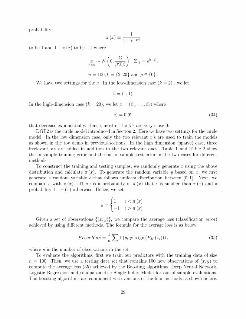
that decrease exponentially. Hence, most of the β’s are very close 0.DGP2 is the circle model introduced in Section 2. Here we have two settings for the circle

model. In the low dimension case, only the two relevant x’s are used to train the modelsas shown in the toy demo in previous sections. In the high dimension (sparse) case, threeirrelevant x’s are added in addition to the two relevant ones. Table 1 and Table 2 showthe in-sample training error and the out-of-sample test error in the two cases for differentmethods.

To construct the training and testing samples, we randomly generate x using the abovedistribution and calculate π (x). To generate the random variable y based on x, we firstgenerate a random variable ε that follows uniform distribution between [0, 1]. Next, wecompare ε with π (x). There is a probability of π (x) that ε is smaller than π (x) and aprobability 1− π (x) otherwise. Hence, we set

y =

1 ε < π (x)

−1 ε > π (x) .

Given a set of observations (x, y), we compare the average loss (classification error)achieved by using different methods. The formula for the average loss is as below.

ErrorRate =1

n

∑1 (yi 6= sign (FM (xi))) , (35)

where n is the number of observations in the set.To evaluate the algorithms, first we train our predictors with the training data of size

n = 100. Then, we use a testing data set that contains 100 new observations of (x, y) tocompute the average loss (35) achieved by the Boosting algorithms, Deep Neural Network,Logistic Regression and semiparametric Single-Index Model for out-of-sample evaluations.The boosting algorithms are component-wise versions of the four methods as shown before.

29

The alternative methods we have, Deep Neural Network, Logistic Regression with LASSOpenalty and semiparametric single-index model with SIM-RODEO considers all variables atthe same time. The number of Monte Carlo repetition for each DGP is 1000.

The results are shown below.

Table 1: Error Rate of Low Dimension Circle Model

Train Error Test ErrorDiscrete AdaBoost 0.0820 0.2053Real AdaBoost 0.0853 0.2038LogitBoost 0.0602 0.2090Gentle AdaBoost 0.0718 0.2062Deep Neural Network 0.2601 0.3533Logistic Regression 0.3586 0.3573SIM-RODEO 0.2986 0.3421

Table 2: Error Rate of High Dimension (Sparse) Circle Model

Train Error Test ErrorDiscrete AdaBoost 0.0202 0.2203Real AdaBoost 0.0295 0.2165LogitBoost 0.0081 0.2232Gentle AdaBoost 0.0133 0.2208Deep Neural Network 0.2838 0.4017Logistic Regression 0.3569 0.3572SIM-RODEO 0.3542 0.3541

Table 3: Error Rate of Low Dimension Logistic Model

Train Error Test ErrorDiscrete AdaBoost 0.1431 0.3129Real AdaBoost 0.1519 0.3120LogitBoost 0.1302 0.3160Gentle AdaBoost 0.1339 0.3154Deep Neural Network 0.2304 0.3090Logistic Regression 0.2773 0.3083SIM-RODEO 0.3069 0.3415

From the simulation results, we can see that the four boosting methods work well in boththe circle model and the logistic model. LogitBoost has the smallest training error among

30

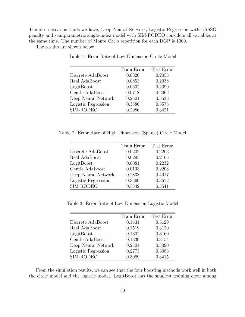
Table 4: Error Rate of High Dimension (Sparse) Logistic Model

Train Error Test ErrorDiscrete AdaBoost 0.0007 0.3217Real AdaBoost 0.0015 0.3215LogitBoost 0.00007 0.3214Gentle AdaBoost 0.0001 0.3204Deep Neural Network 0.0523 0.3172Logistic Regression 0.2328 0.3432SIM-RODEO 0.3580 0.3971

all four boosting algorithms as well as the largest testing error. On the other hand, RealAdaBoost has the largest training error as well as the smallest testing error. Similar rulesapplies to the other two boosting methods. Smaller training errors implies larger testingerrors. This is an evidence of overfitting which is related to the hyper-parameters in theboosting algorithms. If the number of boosting iterations is small, then we will have a largertraining error but less risk of overfitting. On the other hand, if we have more boostingiterations, then the boosting methods will fit the training data better but raise higher riskon overfitting. The number of iterations in the boosting algorithms are fixed by the users.However, cross-validation could be used to determine the optimal number of iterations.

As for the alternative methods, Deep Neural Network works better in the logistic modelthan the circle model. This is a result of the set-up of the Deep Neural Network. We usethe logistic function as the activation function and output function, and the entropy as theloss function. The set-up will give better results when logistic model is the true model. Forthe circle model, Deep Neural Network gives a comparable result to the Logistic Regressionin the low-dimension case. However, the result is much worse for the high-dimension case.Again, this could be a result of our set-up of the Deep Neural Network. We acknowledge thatthe Deep Neural Network is high flexible with lots of hyper-parameters Different set-up ofthe model may lead to dramatically distinct results. Our setting by no means is the optimalone and Deep Neural Network could perform better with a different set-up.

For Logistic Regression, it works best in the low-dimension logistic model as all parametricassumptions are satisfied. However, in the high-dimension case, Logistic Regression will havea larger bias due to the need to shrink the coefficients of irrelevant variables to zero. To fixthis bias, one may try the De-biased Machine Learning method(Chernozhukov et al., 2018).

6 Applications

In this section we illustrate the R functions in two economics applications.In the application, we use the FRED monthly data https://research.stlouisfed.

org/econ/mccracken/fred-databases/ to predict the moving direction of real personalincome in the United States. After removing the observations with missing values, our obtain341 effective observation with a sample period starting from September, 1989 to January

31

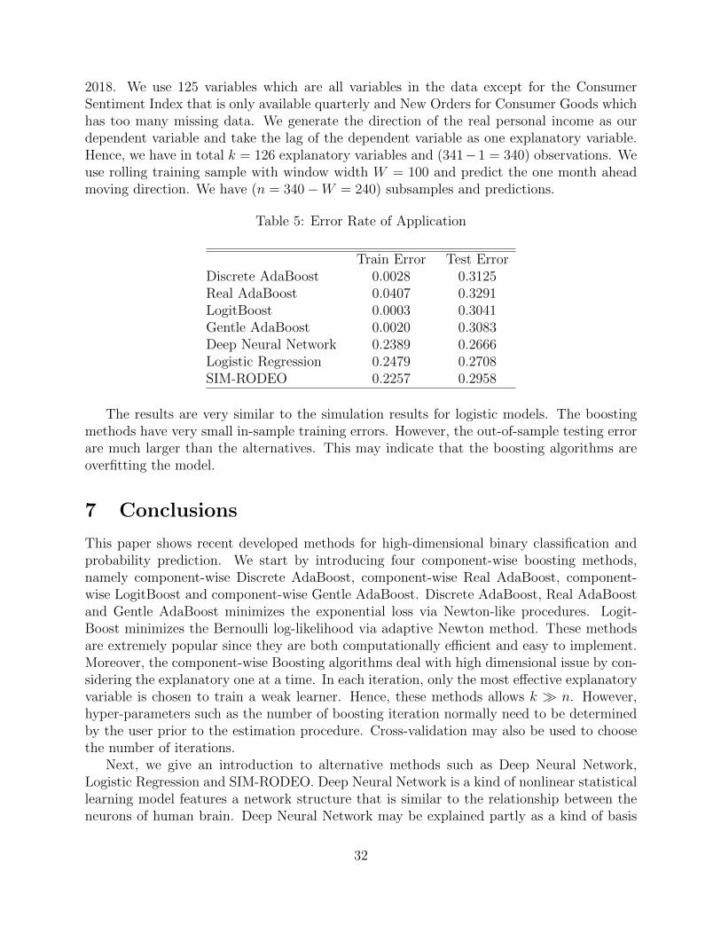
2018. We use 125 variables which are all variables in the data except for the ConsumerSentiment Index that is only available quarterly and New Orders for Consumer Goods whichhas too many missing data. We generate the direction of the real personal income as ourdependent variable and take the lag of the dependent variable as one explanatory variable.Hence, we have in total k = 126 explanatory variables and (341−1 = 340) observations. Weuse rolling training sample with window width W = 100 and predict the one month aheadmoving direction. We have (n = 340−W = 240) subsamples and predictions.

Table 5: Error Rate of Application

Train Error Test ErrorDiscrete AdaBoost 0.0028 0.3125Real AdaBoost 0.0407 0.3291LogitBoost 0.0003 0.3041Gentle AdaBoost 0.0020 0.3083Deep Neural Network 0.2389 0.2666Logistic Regression 0.2479 0.2708SIM-RODEO 0.2257 0.2958

The results are very similar to the simulation results for logistic models. The boostingmethods have very small in-sample training errors. However, the out-of-sample testing errorare much larger than the alternatives. This may indicate that the boosting algorithms areoverfitting the model.

7 Conclusions

This paper shows recent developed methods for high-dimensional binary classification andprobability prediction. We start by introducing four component-wise boosting methods,namely component-wise Discrete AdaBoost, component-wise Real AdaBoost, component-wise LogitBoost and component-wise Gentle AdaBoost. Discrete AdaBoost, Real AdaBoostand Gentle AdaBoost minimizes the exponential loss via Newton-like procedures. Logit-Boost minimizes the Bernoulli log-likelihood via adaptive Newton method. These methodsare extremely popular since they are both computationally efficient and easy to implement.Moreover, the component-wise Boosting algorithms deal with high dimensional issue by con-sidering the explanatory one at a time. In each iteration, only the most effective explanatoryvariable is chosen to train a weak learner. Hence, these methods allows k n. However,hyper-parameters such as the number of boosting iteration normally need to be determinedby the user prior to the estimation procedure. Cross-validation may also be used to choosethe number of iterations.

Next, we give an introduction to alternative methods such as Deep Neural Network,Logistic Regression and SIM-RODEO. Deep Neural Network is a kind of nonlinear statisticallearning model features a network structure that is similar to the relationship between theneurons of human brain. Deep Neural Network may be explained partly as a kind of basis

32

transformation which leads to extreme flexibility of the model. Deep Neural Network and itsvariants are the most popular prediction method at this time and are widely used in fieldssuch as image and voice recognition.

Logistic Regression is a traditional method used intensively in economics for binary clas-sification and probability prediction. Logistic Regression assumes that the probability thatthe output label is 1 conditional on x follows a logistic function of x. Under such assumption,the parameters of the model often has practical economic meaning unlike machine learningmethods that are often hard to interpret. However, logistic regression relies heavily on itsparametric assumptions and is the least flexible model introduced in this paper. In addition,to deal with high-dimensional problem, we have to use the LASSO to control the number ofexplanatory variables chosen in the model.

SIM-RODEO relaxes the parametric assumption of Logistic Regression. As a result,SIM-RODEO is more flexible but, to some extent, still interpretable as Logistic Regression.However, the flexibility of SIM-RODEO may lead to a slower convergence rate and less timeefficiency.

This paper conducted extensive comparison of the above mentioned methods throughMonte Carlo experiments. We compare the methods using both traditional binary classifica-tion model (logistic model) and irregular model (circle model). The boosting methods workwell in both the traditional models and irregular models. Logistic Regression works betterin the low dimension logistic model when the parametric assumptions of Logistic Regressionare satisfied. However, in the high-dimensional case, the LASSO introduces high bias in Lo-gistic Regression and lead to lower classification accuracy. In the irregular models, LogisticRegression performs poor compared to the boosting algorithms. The Deep Neural Networkperformed best in the traditional methods as a result of our configuration of the NeuralNetwork. We acknowledge that our configuration of Deep Neural Network is by no meansthe best and the results here may improve with different activation function, output functionand/or number of hidden layers and neurons. SIM-RODEO is an extension to parametricmethods such as Logistic Regression. It performs reasonably well in the models.

We also use these methods for predicting the changing direction of the real personalincome in the United States. The application show similar results as in the simulation oflogistic models.

This paper gives a thorough introduction of newly developed methods for binary clas-sification and probability prediction. Advantages and disadvantages of each method arediscussed and compared. We conclude that no single method has an absolute advantage inall aspects over the other methods. We believe binary classification and probability predic-tion will remain important for business and economics and look forward to future works onthis problem.

References

Allaire, J., Chollet, F., 2018. keras: R Interface to ’Keras’. URL: https://CRAN.R-project.org/package=keras. r package version 2.1.6.

33

Bliss, C.I., 1934. The method of probits. Science 79, 38–39. URL: http://www.ncbi.nlm.nih.gov/pubmed/17813446, doi:10.1126/science.79.2037.38.

Buhlmann, P., 2006. Boosting for high-dimensional linear models. The Annals of Statistics34, 559–583. doi:10.1214/009053606000000092.

Buhlmann, P., Yu, B., 2003. Boosting with the $L 2$ loss: Regressionand classification. Journal of the American Statistical Association 98, 324–339. URL: http://www.tandfonline.com/doi/abs/10.1198/016214503000125, doi:10.1198/016214503000125.

Chatterjee, S., 2016. fastAdaboost: a Fast Implementation of Adaboost. URL: https:

//CRAN.R-project.org/package=fastAdaboost. r package version 1.0.0.

Chernozhukov, V., Chetverikov, D., Demirer, M., Duflo, E., Hansen, C., Newey, W., Robins,J., 2018. Double/debiased machine learning for treatment and structural parameters.Econometrics Journal 21, C1–C68. URL: http://arxiv.org/abs/1608.00060, doi:10.1111/ectj.12097, arXiv:1608.00060.

Chu, J., Lee, T.H., Ullah, A., 2018a. Asymmetric AdaBoost for High-Dimensional MaximumScore Regression.

Chu, J., Lee, T.H., Ullah, A., 2018b. Variable Selection in Sparse Semiparametric SingleIndex Model.

Cox, D.R., 1958. The regression analysis of binary sequences. Journal of the Royal StatisticalSociety. Series B (Methodological) 20, 215–242. URL: http://www.jstor.org/stable/2983890.

Culp, M., Johnson, K., Michailidis, G., 2016. ada: The R Package Ada for StochasticBoosting. URL: https://CRAN.R-project.org/package=ada. r package version 2.0-5.

Elliott, G., Lieli, R.P., 2013. Predicting binary outcomes. Journal of Econo-metrics 174, 15–26. URL: https://www.sciencedirect.com/science/article/pii/

S0304407613000171, doi:10.1016/j.jeconom.2013.01.003.

Freund, Y., Schapire, R.E., 1997. A Decision-Theoretic Generalization of On-Line Learningand an Application to Boosting. Journal of Computer and System Sciences 55, 119–139.

Friedman, J., Hastie, T., Tibshirani, R., 2000. Additive logistic regression: A statisti-cal view of boosting. Annals of Statistics 28, 337–407. doi:10.1214/aos/1016218223,arXiv:0804.2330.

Friedman, J., Hastie, T., Tibshirani, R., 2010. Regularization Paths for Generalized LinearModels via Coordinate Descent. Journal of Statistical Software 33, 1–22. URL: http://www.jstatsoft.org/v33/i01/, doi:10.18637/jss.v033.i01, arXiv:NIHMS150003.

34

Friedman, J.H., 2001. Greedy Function Approximation: A Gradient Boosting Machine. TheAnnals of Statistics 29, 1189–1232. doi:10.2307/2699986.

Fritsch, S., Guenther, F., 2016. neuralnet: Training of Neural Networks. URL: https:

//CRAN.R-project.org/package=neuralnet. r package version 1.33.

James, G., Witten, D., Hastie, T., Tibshirani, R., 2013. An Introduction to StatisticalLearning with Applications in R. Springer.

Lafferty, J., Wasserman, L., 2008. Rodeo: Sparse, greedy nonparametric regression. Annalsof Statistics 36, 28–63. doi:10.1214/009053607000000811, arXiv:0803.1709.

Lahiri, K., Yang, L., 2012. Forecasting binary outcomes, in: Elliott, G., Timmermann, A.(Eds.), Handbook of Economic Forecasting. SSRN. volume 2, pp. 1025–1106. doi:10.1016/B978-0-444-62731-5.00019-1.

Manski, C.F., 1975. Maximum score estimation of the stochastic utility model ofchoice. Journal of Econometrics 3, 205–228. URL: http://citeseerx.ist.psu.

edu/viewdoc/download?doi=10.1.1.587.6474&rep=rep1&type=pdf, doi:10.1016/0304-4076(75)90032-9.

Manski, C.F., 1985. Semiparametric analysis of discrete response. Asymptotic prop-erties of the maximum score estimator. Journal of Econometrics 27, 313–333. URL: http://citeseerx.ist.psu.edu/viewdoc/download?doi=10.1.1.504.

7329&rep=rep1&type=pdf, doi:10.1016/0304-4076(85)90009-0.

Mease, D., Wyner, A., Buja, A., 2007. Cost-weighted boosting with jittering and over/under-sampling: Jous-boost. Journal of Machine Learning Research 8, 409–439.

Olson, M., 2017. JOUSBoost: Implements Under/Oversampling for Probability Estimation.URL: https://CRAN.R-project.org/package=JOUSBoost. r package version 2.1.0.

R Core Team, 2018. R: A Language and Environment for Statistical Computing. R Foun-dation for Statistical Computing. Vienna, Austria. URL: https://www.R-project.org/.

Ridgeway, G., 2017. gbm: Generalized Boosted Regression Models. URL: https://CRAN.R-project.org/package=gbm. r package version 2.1.3.

Su, L., Zhang, Y., 2014. Variable Selection in Nonparametric and Semiparamet-ric Regression Models, in: Racine, J.S., Su, L., Ullah, A. (Eds.), The OxfordHandbook of Applied Nonparametric and Semiparametric Econometrics and Statis-tics. Oxford University Press. URL: http://www.oxfordhandbooks.com/view/

10.1093/oxfordhb/9780199857944.001.0001/oxfordhb-9780199857944-e-009,doi:10.1093/oxfordhb/9780199857944.013.009.

Tibshirani, R., 1996. Regression Selection and Shrinkage via the Lasso. Journal of theRoyal Statistical Society B 58, 267–288. URL: http://citeseer.ist.psu.edu/viewdoc/summary?doi=10.1.1.35.7574, doi:10.2307/2346178, arXiv:11/73273.

35

Tuszynski, J., 2018. caTools: Tools: moving window statistics, GIF, Base64, ROC AUC,etc. URL: https://CRAN.R-project.org/package=caTools. r package version 1.17.1.1.

Walker, S.H., Duncan, D.B., 1967. Estimation of the probability of an event as a function ofseveral independent variables. Biometrika 54, 167–179. doi:10.1093/biomet/54.1-2.167.

Zou, H., 2006. The Adaptive Lasso and Its Oracle Properties. Journal of the American Sta-tistical Association 101, 1418–1429. URL: http://users.stat.umn.edu/~zouxx019/Papers/adalasso.pdf, doi:10.1198/016214506000000735.

36