Computer Physics Communications 181 (2010) 750–755

Contents lists available at ScienceDirect

Computer Physics Communications

www.elsevier.com/locate/cpc

Complete sets of initial vectors for pattern growth with elementary cellularautomata

Joana G. Freire a,b, Owen J. Brison b,c, Jason A.C. Gallas a,b,d,∗a Instituto de Física, Universidade Federal do Rio Grande do Sul, 91501-970 Porto Alegre, Brazilb Centro de Estruturas Lineares e Combinatórias, Universidade de Lisboa, 1649-003 Lisboa, Portugalc Departamento de Matemática, Faculdade de Ciências, Universidade de Lisboa, 1749-016 Lisboa, Portugald Rechnergestützte Physik der Werkstoffe IfB, ETH Hönggerberg HIF E12, CH-8093 Zürich, Switzerland

a r t i c l e i n f o a b s t r a c t

Article history:Received 22 August 2009Received in revised form 7 December 2009Accepted 8 December 2009

Keywords:Pattern growthCellular automataComplex systemsSpacewise algorithm

Computer simulations of complex spatio-temporal patterns using cellular automata may be performed intwo alternative ways, the better choice depending on the relative size between the spatial width W ofthe expected patterns and their corresponding temporal period T . While the traditional timewise updatingalgorithm is very efficient when W � T , the complementary spacewise algorithm wins whenever T � W .Independently of the algorithm used, the key to obtaining exhaustive answers, not just statisticalestimates, is to have explicit knowledge of the complete sets of initial conditions that need to be individuallytested as sizes grow. This paper reports an efficient algorithm for generating complete sets (withoutredundancy) of k-vectors of initial conditions allowing one to perform definitive classifications of patternsin systems with a minimal characteristic length k, either spatial or temporal.

© 2009 Elsevier B.V. All rights reserved.

1. Introduction

The simulation of complex spatio-temporal patterns using cel-lular automata may be performed in two complementary ways: ei-ther by applying the traditional timewise updating algorithm [1–5],or by applying a complementary spacewise updating [6,7]. In bothcases, the critical information required to start simulations is a setof initial conditions defining the initial state of the automaton. Evenafter discounting trivial repetitions, the number of initial condi-tions grows exponentially fast with the lattice size k. For instance,for the simplest possible class of automata, namely for binary au-tomata,1 an upper bound for the number nu(k) of initial conditionsthat need to be explicitly investigated to find exhaustively all pos-sible dynamical behaviors of the automaton is nu(k) = 2k . Thisquantity provides simultaneously an estimate of the size of thesampling space that needs to be probed, as well as an indicationof the computational complexity of the search that needs to beperformed.

In many applications, particularly in statistical physics, one isinterested in the dynamics at the so-called thermodynamic limit,i.e. the limit k → ∞. The problem of investigating accurately thethermodynamic limit is that the exponential growth of the di-mension of the sampling space frequently prevents an exhaustive

* Corresponding author.E-mail address: jgallas@if.ufrgs.br (J.A.C. Gallas).

1 A binary automaton is one in which individual cells may assume one of twopossible values.

0010-4655/$ – see front matter © 2009 Elsevier B.V. All rights reserved.doi:10.1016/j.cpc.2009.12.007

search of all possible patterns supported even by the most elemen-tary binary automata. So, instead of accurate exhaustive results, thethermodynamic limit forces one to be content with just statisticalestimates of the asymptotic behaviors. This difficulty by no meansprevented the useful application of cellular automata to many sit-uations of interest in several disciplines, as amply described inseveral books and in the technical literature [1–5].

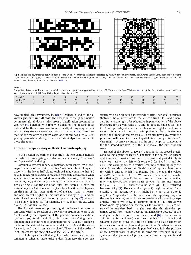
A totally different class of applications focuses not on thethermodynamic limit but on the simulation of complex spatio-temporal patterns and, with particular emphasis, on classifyingexhaustively all patterns supported by specific rules. Of great in-terest are temporally periodic patterns like those typically presentin, say, models of crystal growth or in the so-called “gliders”, i.e.in spatially localized or traveling structures characteristic of com-plex “class 4” automaton rules [1,4]. Three representative examplesof gliders are shown in Fig. 1, generated by rule 20, a popularrule among those known for their complex dynamics [8–12]. Un-der rule 20, the state of any given site i at time t + 1 depends onthe state of the site at time t as well as on the state of its nearestand next-nearest neighbors through the sum

Σi(t) ≡ σi−2(t) + σi−1(t) + σi(t) + σi+1(t) + σi+2(t) (1)

and is synchronously updated as follows:

σi(t + 1) ={

1 if Σi(t) ∈ I,0 otherwise.

(2)

For rule 20, the set I contains just two numbers, namely I = {2,4}.Fig. 1 illustrates the asymmetry T � W frequently observed be-

tween the period T and width W of complex gliders. To quantify

J.G. Freire et al. / Computer Physics Communications 181 (2010) 750–755 751

Fig. 1. Typical size asymmetries between period T and width W observed in gliders supported by rule 20. Time runs vertically downwards. Left column, from top to bottom:(T , W ) = (4,21), (4,22), (5,37). Right column: example of a situation with (T , W ) = (38,31). The left column illustrates situations where T � W while in the right weshow the only known glider with T > W (see Table 1).

Table 1Comparison between width and period of all known static patterns supported by the rule 20. Values taken from Wolfram [4], except for the situation marked with anasterisk, reported in Ref. [7]. Note that only one glider has T > W .

Period T 1 2 3 4 4 5 6 6∗ 8 10 10 10 22 38Width W 8 9 42 21 22 37 66 73∗ 45 57 61 73 28 31W − T 7 7 39 17 18 32 60 67∗ 37 47 51 63 6 −7

how “typical” this asymmetry is, Table 1 collects T and W for allknown gliders of rule 20. With the exception of the glider markedby an asterisk, all data is taken from a classification presented byWolfram [4], obtained with timewise updating. The missing gliderindicated by the asterisk was found recently during a systematicsearch using the spacewise algorithm [7]. From Table 1 one seesthat for the majority of known cases one indeed has T � W , sug-gesting spacewise updating to be the efficient algorithm to used inthese situations.

2. The two complementary methods of automata updating

In this section we outline and contrast the two complementarymethods for investigating cellular automata, namely “timewise”and “spacewise” updating.

Consider a general binary automaton, represented by a rect-angular matrix of indefinite size (an “indefinite sheet of squaredpaper”) in the lower half-plane; each cell may contain either a 0or a 1. Temporal evolution is recorded vertically downwards whilespatial dimension is recorded horizontally, increasing to the right.Denote by σi(t) the state (or value) of the automaton at (spatial)site i at time t . For the evolution rules that interest us here, thestate of any site i at time t + 1 is given by a function that dependson the sum of the states at time t of the site i and its nearestand next-nearest neighbors. This sum is defined by Eq. (1) and thestate of each site i is synchronously updated by Eq. (2), where Iis a suitably-defined set; for example, I = {2,4} for rule 20, whileI = {2,4,5} for rule 52, etc.

The classical timewise updating algorithm for such an automa-ton starts with the selection of a convenient spatial dimension, sayL cells, and by the imposition of the periodic boundary conditionσi(t) = σi+L(t) for all i and all t; this amounts to defining the au-tomaton on a cylinder whose circumference has L cells. A choice ismade for the state of the automaton at time t = 0 and the valuesfor t = 1, t = 2, and so on, are calculated. There are of the order of2L/L choices for the state at t = 0: see Ref. [7] for details.

One of the questions that might be asked about such an au-tomaton is whether there exist gliders (non-zero time-periodic

structures on an all-zero background) or (time-periodic) interfaces(between the all-zero state to the left of a fixed site i and a non-zero state to the right). An exhaustive implementation of the aboveprocedure for a given value of L and all possible choices for timet = 0 will probably discover a number of such gliders and inter-faces. This approach has two main problems: for L moderatelylarge, the number of choices for t = 0 becomes unwieldy, while theprocedure will miss structures of spatial dimension greater than L.One might successively increase L in an attempt to compensatefor the second problem, but this just makes the first problemworse.

Instead of the above “timewise” updating, it has proved practi-cable to implement “spacewise” updating in the search for glidersand interfaces, provided we first fix a temporal period k. Typi-cally, we start on the left with σi(t) = 0 for 1 � i � 4 and forall t; this corresponds to 4 vertical columns containing only thevalue 0. We then choose an “initial vector” vk , a column vec-tor with k entries which are, reading from the top, the valuesof σ5(t) for t = 0, . . . ,k − 1. We impose the periodicity condi-tion that σi(t) = σi(t + k) for all i and all t . We then note thatif σi(t) is known, and if the values of σ j(t − 1) are also knownfor j = i − 2, . . . , i + 1, then the value of σi+2(t − 1) is restrictedbecause of Eq. (2). The value of σi+2(t − 1) might be either “nec-essarily 0” or “necessarily 1”, it might be “either 0 or 1”, or itmight be “impossible”. In the latter case, the updating stops. Inthe ambiguous case, we will have to develop each possibility sep-arately. Thus if we know all columns up to i + 1, then as weknow σi(k) by periodicity, the values for column i + 2 are re-stricted as just described. It might seem that this sidewise up-dating would itself rapidly become unmanageable because of theambiguities, but in practice we have found [6] it to be work-able. It can be (and was) even used by hand with pencil andsquared paper to prove that rule 52 admits no static gliders orinterfaces of minimal temporal period 4 or 5, when all side-wise updatings ended in the “impossible” case. It is the purposeof the present work to describe an algorithm, recursive in k, tosystematically generate all possible initial vectors vk mentionedabove.

752 J.G. Freire et al. / Computer Physics Communications 181 (2010) 750–755

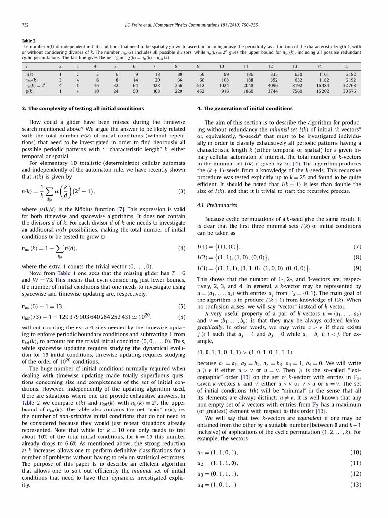
Table 2The number n(k) of independent initial conditions that need to be spatially grown to ascertain unambiguously the periodicity, as a function of the characteristic length k, withor without considering divisors of k. The number ntot(k) includes all possible divisors, while nu(k) ≡ 2k gives the upper bound for ntot(k), including all possible redundantcyclic permutations. The last line gives the net “gain” g(k) ≡ nu(k) − ntot(k).

k 2 3 4 5 6 7 8 9 10 11 12 13 14 15

n(k) 1 2 3 6 9 18 30 56 99 186 335 630 1161 2182ntot(k) 3 4 6 8 14 20 36 60 108 188 352 632 1182 2192nu(k) ≡ 2k 4 8 16 32 64 128 256 512 1024 2048 4096 8192 16 384 32 768g(k) 1 4 10 24 50 108 220 452 916 1860 3744 7560 15 202 30 576

3. The complexity of testing all initial conditions

How could a glider have been missed during the timewisesearch mentioned above? We argue the answer to be likely relatedwith the total number n(k) of initial conditions (without repeti-tions) that need to be investigated in order to find rigorously allpossible periodic patterns with a “characteristic length” k, eithertemporal or spatial.

For elementary 1D totalistic (deterministic) cellular automataand independently of the automaton rule, we have recently shownthat n(k) is given by

n(k) = 1

k

∑d|k

μ

(k

d

)(2d − 1

), (3)

where μ(k/d) is the Möbius function [7]. This expression is validfor both timewise and spacewise algorithms. It does not containthe divisors d of k. For each divisor d of k one needs to investigatean additional n(d) possibilities, making the total number of initialconditions to be tested to grow to

ntot(k) = 1 +∑d|k

n(d), (4)

where the extra 1 counts the trivial vector (0, . . . ,0).Now, from Table 1 one sees that the missing glider has T = 6

and W = 73. This means that even considering just lower bounds,the number of initial conditions that one needs to investigate usingspacewise and timewise updating are, respectively,

ntot(6) − 1 = 13, (5)

ntot(73) − 1 = 129 379 903 640 264 252 431 � 1020, (6)

without counting the extra 4 sites needed by the timewise updat-ing to enforce periodic boundary conditions and subtracting 1 fromntot(k), to account for the trivial initial condition (0,0, . . . ,0). Thus,while spacewise updating requires studying the dynamical evolu-tion for 13 initial conditions, timewise updating requires studyingof the order of 1020 conditions.

The huge number of initial conditions normally required whendealing with timewise updating made totally superfluous ques-tions concerning size and completeness of the set of initial con-ditions. However, independently of the updating algorithm used,there are situations where one can provide exhaustive answers. InTable 2 we compare n(k) and ntot(k) with nu(k) ≡ 2k , the upperbound of ntot(k). The table also contains the net “gain” g(k), i.e.the number of non-primitive initial conditions that do not need tobe considered because they would just repeat situations alreadyrepresented. Note that while for k = 10 one only needs to testabout 10% of the total initial conditions, for k = 15 this numberalready drops to 6.6%. As mentioned above, the strong reductionas k increases allows one to perform definitive classifications for anumber of problems without having to rely on statistical estimates.The purpose of this paper is to describe an efficient algorithmthat allows one to sort out efficiently the minimal set of initialconditions that need to have their dynamics investigated explic-itly.

4. The generation of initial conditions

The aim of this section is to describe the algorithm for produc-ing without redundancy the minimal set I(k) of initial “k-vectors”or, equivalently, “k-seeds” that must to be investigated individu-ally in order to classify exhaustively all periodic patterns having acharacteristic length k (either temporal or spatial) for a given bi-nary cellular automaton of interest. The total number of k-vectorsin the minimal set I(k) is given by Eq. (4). The algorithm producesthe (k + 1)-seeds from a knowledge of the k-seeds. This recursiveprocedure was tested explicitly up to k = 25 and found to be quiteefficient. It should be noted that I(k + 1) is less than double thesize of I(k), and that it is trivial to start the recursive process.

4.1. Preliminaries

Because cyclic permutations of a k-seed give the same result, itis clear that the first three minimal sets I(k) of initial conditionscan be taken as

I(1) = {(1), (0)

}, (7)

I(2) = {(1,1), (1,0), (0,0)

}, (8)

I(3) = {(1,1,1), (1,1,0), (1,0,0), (0,0,0)

}. (9)

This shows that the number of 1-, 2-, and 3-vectors are, respec-tively, 2, 3, and 4. In general, a k-vector may be represented byu = (a1, . . . ,ak) with entries a j from F2 = {0,1}. The main goal ofthe algorithm is to produce I(k + 1) from knowledge of I(k). Whenno confusion arises, we will say “vector” instead of k-vector.

A very useful property of a pair of k-vectors u = (a1, . . . ,ak)

and v = (b1, . . . ,bk) is that they may be always ordered lexico-graphically. In other words, we may write u > v if there existsj � 1 such that a j = 1 and b j = 0 while ai = bi if i < j. For ex-ample,

(1,0,1,1,0,1,1) > (1,0,1,0,1,1,1)

because a1 = b1, a2 = b2, a3 = b3, a4 = 1, b4 = 0. We will writeu � v if either u > v or u = v . Then � is the so-called “lexi-cographic” order [13] on the set of k-vectors with entries in F2.Given k-vectors u and v , either u > v or v > u or u = v . The setof initial conditions I(k) will be “minimal” in the sense that allits elements are always distinct: u = v . It is well known that anynon-empty set of k-vectors with entries from F2 has a maximum(or greatest) element with respect to this order [13].

We will say that two k-vectors are equivalent if one may beobtained from the other by a suitable number (between 0 and k−1inclusive) of applications of the cyclic permutation (1,2, . . . ,k). Forexample, the vectors

u1 = (1,1,0,1), (10)

u2 = (1,1,1,0), (11)

u3 = (0,1,1,1), (12)

u4 = (1,0,1,1) (13)

J.G. Freire et al. / Computer Physics Communications 181 (2010) 750–755 753

form a complete class of equivalent vectors which is ordered lexi-cographically as follows:

u2 > u1 > u4 > u3.

We take u2, the maximum element with respect to the lexico-graphic order, as the representative of the class. It is clear that,apart from the “exceptional” vectors (1, . . . ,1) and (0, . . . ,0), achosen representative (a1, . . . ,ak) of an equivalence class will al-ways have a1 = 1 and ak = 0.

From Eqs. (7)–(9) one might have the impression that I(k + 1)

may be obtained from I(k) by adjoining a 1 to the left side of eachvector of I(k) and finally adding the vector (0, . . . ,0). However,I(4) is given by

I(4) = {(1,1,1,1), (14)

(1,1,1,0), (15)

(1,1,0,0), (16)

(1,0,1,0), (17)

(1,0,0,0), (18)

(0,0,0,0)}. (19)

From this, one sees that the vector (1,0,1,0) is not obtained fromI(3) by the above procedure. Note that (1,0,1,0) is a repetition ofthe 2-vector (1,0). In other words, we may consider that (1,0) isa divisor of (1,0,1,0) as 2 divides 4.

We say that a k-vector v has minimal period d if d is the small-est number such that v is invariant under a cyclic-shift of d places;such a d must be a divisor of k.

The set I(k) is formed by the union of two disjoint sets

I(k) = N(k) ∪ D(k). (20)

The first set, N(k), is the set of all initial vectors which correspondto minimal period k. That is, N(k) is the complete set of chosenrepresentatives of the various classes of those vectors that corre-spond to minimal period k. The second set D(k) is related withthe divisors of k. If d is a divisor of k with 1 � d < k then certaink-vectors correspond to minimal period d. From each equivalenceclass of vectors with minimal period d where 1 � d < k we choosethe maximal vector with respect to the lexicographic order as therepresentative, and write D(k) for the set of all such representa-tives. We include the case d = 1, which corresponds to the k-vector(1, . . . ,1). The vector (0, . . . ,0) belongs to D(k) because it is in-variant under shifts by 1 place.

For any v ∈ I(k) we define b ≡ b(v) as the size of a maximalblock of cyclically-consecutive entries which are all equal to 1 inthe vector v . For example, if v = (1,0,0,1,1) then b = 3 because,due to the boundary conditions, we consider the three entries “1”to be cyclically-consecutive, while if v = (1,0,1,1,0) then b = 2.

Next, for a given v ∈ I(k) one needs to be able (1) to calcu-late b; (2) to locate all blocks of b(v) cyclically-consecutive 1sin v; (3) provided that b � 1, to find the blocks of exactly b − 1cyclically-consecutive entries equal to 1, if any. In this context, a“block of exactly 0 entries equal to 1” is defined to be an entryequal to 0.

It may happen that v possesses more than one block of bcyclically-consecutive entries equal to 1. For example, if v =(1,1,1,0,1,1,1,0,1,0,0) then b = 3 and v possesses 2 blocksof 3 cyclically-consecutive entries equal to 1.

If v possesses just one block of b cyclically-consecutive en-tries equal to 1, we will say that v possesses a “unique maxi-mal block” and we will say that v is a UMB vector. For example,v1 = (1,0,1,1,1,0,1,0,0,1) is a UMB vector with b = 3.

If a vector v is a UMB vector and if its unique maximalblock is situated at the beginning (i.e. at the left-hand end)

of v , then v must be an initial vector because v is greater (inthe lexicographic order) that any shift of v . For example, v2 =(1,1,1,0,1,0,0,1,1,0) is an initial vector of I(10) with b = 3.Obviously, v2 may be obtained by performing two shifts on v1above.

If a vector v is initial it must commence with a maximalblock of b consecutive entries equal to 1, because of the lexi-cographic order, but it need not be a UMB vector. For example,v = (1,1,1,0,1,1,1,0,0,0) is an initial 10-vector. Here b = 3 andv has two blocks of 3 cyclically-consecutive entries equal to 1.

4.2. The algorithm

It is assumed that a lexicographically ordered I(k) is known forsome k � 1. As mentioned before, the aim is to generate an or-dered I(k + 1) from the knowledge of I(k).

For convenience, during the computation we will use I(k + 1)

as a place-holder for the vectors generated, possibly containing re-dundancies. Such redundancies will be eliminated by performing alexicographic ordering at the end.

Start by adjoining a 1 to (0, . . . ,0) ∈ I(k) to get (1,0, . . . ,0) ∈I(k + 1). Add the (k + 1)-vector (0, . . . ,0) to I(k + 1).

Proceeding in lexicographic order, for each v = (a1, . . . ,ak) ∈I(k), v = (0, . . . ,0), determine the value of b = b(v). Further, cal-culate the minimum period, d, to which v corresponds; d is nec-essarily a divisor of k (possibly equal to k). Store this minimumperiod d. By definition of b(v), v has one or more maximal blocksof exactly b = b(v) consecutive 1s. In particular, provided v = (0,

. . . ,0), v must begin with a maximal block of b � 1 consecutiveentries equal to 1. After this, the algorithm consists essentially ofperforming two tasks:

(a) Shift v successively through 0,1, . . . , i, . . . ,d − 1 places to ob-tain vectors v0 = v, v1, . . . , vi, . . . , vd−1. For each i = 0, . . . ,

d − 1, check to see if vi starts with a block of b consecutive1s.2 If vi starts with a block of b consecutive 1s, adjoin a 1 toobtain (1, vi). This vector must start with a unique maximalblock of (b + 1) 1s and so must be initial. Place this vector(1, vi) into I(k + 1). If vi does not start with a block of b con-secutive 1s, proceed to the next i.

(b) Check whether v has one or more blocks of exactly b − 1 con-secutive 1s. If so, then shift v an appropriate number of timesup to a maximum of d − 1 places so that each such block, inits turn, appears at the front. After each such shift, test to seewhether the resulting vector, v ′ , ends in a 0 or a 1. If the vec-tor v ′ ends in 1, then discard it3; else create a (k + 1)-vectorv ′

1 by adjoining a 1 at the front. After that: Test to see whetherv ′

1 is initial or not: If it is not initial, discard it.4 If v ′1 is initial,

add it to the set I(k + 1).

Proceed to the next v ∈ I(k).Finally, put the vectors of I(k + 1) into lexicographic order. This

ends the algorithm. Note that in step (a), all (k + 1)-vectors pro-duced are distinct and are UMB vectors. Step (b) never produces

2 Of course, v0 does.3 It might seem that this should not occur; it will not if b � 2, but might occur

if b = 1 because a block of exactly 0 1s is, by our definition, a 0. For example,(0,1,0) → (1,0,1,0) but (0,0,1) is discarded. The potential new vector if (0,0,1)

was not discarded, (1,0,0,1), is equivalent to the vector we obtain by adding 1 tothe front of (1,0,0).

4 There is no need here to shift v ′1 to get an initial vector in I(k + 1): such an

initial vector will arise elsewhere. For example, suppose v = (1,1,0,1,0,0) ∈ I(6).Here, b(v) = 2. Shift to v ′ = (1,0,0,1,1,0). Adjoin 1 to get v ′

1 = (1,1,0,0,1,1,0).This vector is not initial: its initial representative is w = (1,1,0,1,1,0,0). However,w arises by adjoining 1 to (1,0,1,1,0,0) and this is a shift of (1,1,0,0,1,0) ∈ I(6)

and so we will obtain w anyway.

754 J.G. Freire et al. / Computer Physics Communications 181 (2010) 750–755

UMB vectors and so there is no possibility that vectors from (a)and (b) might coincide.

Examples.

(i) Take v = (1, . . . ,1) ∈ I(k). Then step (a) gives (1,1, . . . ,1) ∈I(k + 1).

(ii) Take v = (1,1,0,1,1,0,0) ∈ I(7). Then step (a) gives distinctvectors (1,1,1,0,1,1,0,0) and (1,1,1,0,0,1,1,0) ∈ I(8).

(iii) Consider k = 14 and v = (1,1,0,1,1,0,0,1,1,0,1,1,0,0) ∈I(14), period d = 7. We append a 1 to the front of v toget (1,1,1,0,1,1,0,0,1,1,0,1,1,0,0) ∈ I(15). If we were toshift v by 7 places the result would be v again, which is ofno further interest; we avoided this by only shifting v through0,1, . . . ,d − 1 places. However, a shift of 3 places gives v3 =(1,1,0,0,1,1,0,1,1,0,0,1,1,0) = v; when we adjoin a 1 tothe front of v3 we get (1,1,1,0,0,1,1,0,1,1,0,0,1,1,0) ∈I(15), and this is different to the vector found above. All otherpossible shifts will give either v or v3 or else a vector thatdoes not start with a block of 2 1s. For example, a shift of 10places gives (1,1,0,0,1,1,0,1,1,0,0,1,1,0).

Example. Take v = (1,0,0,1,0,1,0), with b = 1. Each of the 4entries equal to 0 counts as a block of b − 1 = 0 consecutive 1s.We will shift each in turn to the front:

(0,0,1,0,1,0,1)

(0,1,0,1,0,1,0)

(0,1,0,1,0,0,1)

(0,1,0,0,1,0,1).

Of these, we discard the first, third and fourth. We take thesecond, v ′ = (0,1,0,1,0,1,0), and adjoin a 1 at the front: v ′

1 =(1,0,1,0,1,0,1,0). This vector is initial and has d = 2; we placeit in I(8).

Step (b) in the above algorithm may be replaced by the follow-ing alternative step:

(b) (alternative) Check whether v has one or more blocks ofexactly b − 1 consecutive 1s. If so, then if b = 1 then shift v (up toa maximum of d − 1 places) so that each 0 in succession appearsat the front, to give vectors generically called v ′ . If v ′ ends in 1then discard it. Otherwise create a (k + 1)-vector v ′

1 by adjoining1 to the front of v ′ . Test to see if v ′

1 is initial; if so, place it inI(k + 1) and if not, discard it. On the other hand, if b � 2 shift v(up to a maximum of d − 1 places) so that each block of b − 1cyclically-consecutive 1s, in its turn appears at the front.5 On eachoccasion, create a (k + 1)-vector v ′

1 by adjoining a 1 at the frontof v ′ . Check to see whether v ′

1 is initial. If it is initial, add it to theset I(k + 1), otherwise discard it.

Proceed to the next v ∈ I(k).To conclude this section, we remark that although convenient

for humans, lexicographic order is not strictly necessary for themachine. In fact, the ordering may be omitted without altering thefinal results. What matters is that each vector be a representativeof its class.

5. Validation

The purpose of this section is to show that the above algorithm:(1) produces I(k + 1) containing a complete set of initial vectors,and (2) does not give repetitions.

5 After each rotation, the resulting vector, v ′ , must end in a 0 because b > 1.

(1) Suppose that v1 ∈ I(k + 1), v1 = (1,0, . . . ,0) and v1 = (0,0,

. . . ,0). We wish to show that v1 arises from some vector v ∈I(k) in either (a) or (b) above. We may also assume v1 = (1,1,

. . . ,1) because this vector is produced by (a) from the k-vector(1, . . . ,1) ∈ D(k).

Thus v1 starts with b = b(v1) � 1 consecutive 1s, followed byat least one 0.

If there are no other blocks of b consecutive 1s in v1 then v1arises by adjoining a 1 to the left of a k-vector v where b(v) =b − 1 and such that v starts with a block of b − 1 consecutive 1s;such a vector v can, if necessary, be shifted to a vector v∗ ∈ I(k)

and so v1 will have been constructed in (a) or (b).Suppose that v1 possesses further blocks of b consecutive 1s.

Again, v1 arises by appending a 1 to the left of a k-vector v . Inthis case, b(v) = b and v must have started with a block of b − 1consecutive 1s; such a vector v can be shifted to give a vector v∗which starts with a block of b consecutive 1s and which belongsto I(k), so that v1 arises in (b).

(2) In (a) and (b) we produce new vectors by appending a 1 tothe left of vectors which are shifts, by at most d − 1 places (whered is the minimum period) of vectors in I(k). Suppose the vector v1has been produced by appending a 1 to the left of a k-vector v .Then v is equivalent to a vector v∗ ∈ I(k), and arises only oncein the process of successively shifting v∗ by 0,1, . . . ,d − 1 places.It follows that the vectors produced in the algorithm are distinctamong themselves.

6. Algorithm overview

We now give an abridged description of the algorithm of Sec-tion 4.2. This abridged version generates the same set generated bythe algorithm of Section 4.2. It is however shorter because it relieson concepts and notation introduced in the previous sections. Asabove, the goal is to generate I(k + 1) assuming that the lexico-graphically ordered set I(k) is known.

Apart from the “exceptional” vectors (1, . . . ,1) and (0, . . . ,0),a representative vector (v1, . . . , vk) will always have v1 = 1 andvk = 0.

The algorithm consists of the following steps:

1. Adjoin 1 to the exceptional vector (0, . . . ,0) to get (1,0, . . . ,0)

and place this vector in I(k + 1). Place the (k + 1)-vector(0, . . . ,0) into I(k + 1).

2. For each vector v ∈ I(k) we need to:(a) Calculate the minimal period d of v .(b) Calculate b ≡ b(v), defined as the size of a maximal block

of cyclically-consecutive entries which are all equal to 1 inthe vector v .

(c) Locate all blocks of b cyclically-consecutive 1s in the firstd places of v .

(d) Provided that b � 1, locate all the blocks of exactly b − 1cyclically-consecutive entries equal to 1 in the first dplaces of v .

(e) Shift each block of size b found in (c) to the leftmost posi-tion and produce new vectors v1 ∈ I(k + 1) by appendinga 1 to the left of the shifted vectors v ∈ I(k). Drop all non-initial vectors, if any.

(f) If b � 1 and if (b −1)-blocks exist, repeat (e) but for all theblocks with b − 1 cyclically-consecutive entries equal to 1found in (d). Drop all non-initial vectors, if any.

3. Order I(k + 1) lexicographically.

7. Conclusions and outlook

In conclusion, we have presented an explicit algorithm to gen-erate recursively complete sets of initial conditions that need to be

J.G. Freire et al. / Computer Physics Communications 181 (2010) 750–755 755

tested individually in order to obtain exhaustive classification ofpatterns, not mere statistical estimates. The algorithm may be ap-plied equally well to classify spatial or temporal patterns in sys-tems with a minimal characteristic length k. From the discussionin Section 3 and a comparison between the numbers given inEqs. (5) and (6) one realizes that the choice of an adequate up-dating algorithm plays a decisive role: while the thermodynamiclimit is certainly out of reach for exhaustive classifications, muchremains to be discovered regarding the classification of periodicpatterns with finite sizes. In particular, spacewise updating mightbe now efficiently used to grow patterns under rules of arbitrarycomplexity. A recent systematic search combining the spacewiseupdating algorithm with a brute force scan of the initial con-ditions has produced unexpected results, revealing patterns thatwere so far overlooked in previous classifications [7]. Now, usingthe minimal set of initial conditions as described here, it shouldbe possible to conduct much wider searches of complex patternswith longer periods. It should be also possible to adapt the space-wise updating algorithm to classify automatically traveling glidersand to investigate what sort of gliders are capable of surviving re-peated collisions in the lattice and, thus, may be used as carriersof useful information across extended spatial domains. The presentalgorithm combined with spacewise search is also expected to helpfinding exhaustive answers concerning the spatio-temporal orga-nization of cellular automaton models of interesting applicationssuch as, for example, computer networks [14–17], secure schemesto share encrypted color images [18], modeling of biological pat-terns and processes like, e.g., tumor growth [19,20], efficient meansof simulating mixing and segregation of granular media [21] aswell as in a number of fundamental open questions in physics[22–31].

Acknowledgements

J.G.F. thanks Fundação para a Ciência e Tecnologia, Portugal, fora Postdoctoral Fellowship and Instituto de Física da UFRGS for hos-pitality. O.J.B. and J.A.C.G. thank the Centro de Estruturas Lineares eCombinatórias, Universidade de Lisboa, for partial support. J.A.C.G.thanks Hans J. Herrmann for a fruitful month spent in his Institutein Zürich. He is supported by the Air Force Office of Scientific Re-search, Grant FA9550-07-1-0102, and by CNPq, Brazil. The authorsthank CESUP-UFRGS for access to the Sun Fire X2200 and X4600clusters.

Appendix A. MAPLE code for computing n(k) and ntot(k)

The following MAPLE code evaluates Eqs. (3) and (4) and maybe used to extend Table 2. The program is set here to generate allvalues of n(k) and ntot(k) up to k = 73, the value given in Eq. (6).It runs in a small fraction of a second. It is instructive to run it andsee how fast these numbers grow.

with(numtheory):n(1) := 1:n(2) := 1:for k from 3 to 73 dopdiv := divisors(k)[1..(tau(k)-1)]:

sr(k) :=0:ntot(k) :=1:

for d in pdiv do sr(k):=sr(k)+d*n(d) od:n(k) := (2^k - (sr(k)+1))/k:

pdiv := divisors(k);for d in pdiv do ntot(k):=ntot(k)+n(d) od:print( k, n(k), ntot(k) );

od:

Alternatively, one may also use a MAPLE function to obtain n(k)

as follows:

with(numtheory):for k from 1 to 73 dopdiv := divisors(k); soma(k) := 0:for d in pdiv do

soma(k):=soma(k)+mobius(k/d)*(2^d - 1) od:n(k) := soma(k)/k:print( k, n(k) );

od:

References

[1] B. Chopard, M. Droz, Cellular Automata Modeling of Physical Systems, Cam-bridge University Press, Cambridge, 1998.

[2] R. Badii, A. Politi, Complexity: Hierarchical Structures and Scaling in Physics,Cambridge University Press, Cambridge, 1997.

[3] A. Ilachinski, Cellular Automata, World Scientific, Singapore, 2001.[4] S. Wolfram, A New Kind of Science, Wolfram Media, Champaign, 2002.[5] For recent surveys see: A.E. Motter, Z. Toroczkai (Eds.), Focus Issue: Optimiza-

tion in Networks, Chaos 17 (2007);S. Havlin, M. Nekovee, Y. Moreno (Eds.), Focus on Complex Networked Systems:Theory and Application, New J. Phys. 9 (2007).

[6] J.G. Freire, O.J. Brison, J.A.C. Gallas, Chaos 17 (2007) 026113.[7] J.G. Freire, O.J. Brison, J.A.C. Gallas, J. Phys. A: Math. Theor. 42 (2009) 395003.[8] S. Wolfram, Physica D 10 (1984) 1.[9] J.A.C. Gallas, H.J. Herrmann, Internat. J. Modern Phys. C 1 (1990) 181.

[10] J.A.C. Gallas, P. Grassberger, H.J. Herrmann, P. Ueberholz, Physica A 180 (1992)19.

[11] J.A.C. Gallas, H.J. Herrmann, Physica A 356 (2005) 78.[12] J.G. Freire, J.A.C. Gallas, Phys. Lett. A 366 (2007) 25.[13] G. James, A. Kerber, The Representation Theory of the Symmetric Group,

Addison-Wesley, New York, 1981, p. 23.[14] Z. Ren, Z. Deng, Comput. Phys. Comm. 144 (2002) 243, 310.[15] D.A. Meyer, Comput. Phys. Comm. 146 (2002) 295.[16] C.R. Calidonna, S. Di Gregorio, M.M. Furnari, Comput. Phys. Comm. 147 (2002)

724.[17] D.R. Paula, A.D. Araujo, J.S. Andrade, H.J. Herrmann, J.A.C. Gallas, Phys. Rev. E 74

(2006) 017102.[18] G. Alvarez, A. Hernández Encinas, L. Hernández Encinas, A. Martín del Rey,

Comput. Phys. Comm. 173 (2005) 9.[19] A. Deutsch, S. Dormann, Cellular Automaton Modeling of Biological Pattern For-

mation, Birkhäuser, Basel, 2005.[20] P. Gerlee, A.R.A. Anderson, J. Theoret. Biol. 259 (2009) 67.[21] D.V. Ktitarev, D.E. Wolf, Comput. Phys. Comm. 121–122 (1999) 303.[22] B.L. Costello, R. Toth, C. Stone, A. Adamatzky, L. Bull, Phys. Rev. E 79 (2009)

026114.[23] T. Kahle, E. Olbrich, J. Jost, N. Ay, Phys. Rev. E 79 (2009) 026201.[24] F. Bagnoli, R. Rechtman, Phys. Rev. E 79 (2009) 041115.[25] C.R. Shalizi, R. Haslinger, J.-B. Rouquier, K.L. Klinkner, C. Moore, Phys. Rev. E 73

(2006) 036104.[26] H. Janicke, A. Wiebel, G. Scheuermann, W. Kollmann, IEEE Trans. Visualization

Computer Graphics 13 (2007) 1384.[27] J.T. Lizier, M. Prokopenko, A.Y. Zomaya, Phys. Rev. E 77 (2008) 026110.[28] M. Prokopenko, F. Boschetti, A.J. Ryan, Complexity 15 (2009) 11.[29] A.B. Bracic, I. Grabec, E. Govekar, Eur. Phys. J. B 69 (2009) 529.[30] B. Fernandez, B. Luna, E. Ugalde, Phys. Rev. E 80 (2009) 025203.[31] M. Gonzalez, D. Dominguez, F.B. Rodriguez, Neurocomputing 72 (2009) 3795.