comparison of two matrix data structures for advanced … · comparison of two matrix data...
TRANSCRIPT
r
NASA Contractor Report 181951
Comparison of Two Matrix Data Structuresfor Advanced CSM Testbed Applications
M. E. Regelbrugge, F. A. Brogan,
B. Nour-Omid, C. C. Rankin, and M. A. Wright
Lockheed Missiles and Space Company, Inc.
Pa]o Alto, CA 94304
Contract NAS1-18444
December 1989
NASANational Aeronautics andSpace Administration
Langley Research CenterHampton, Virginia 23665-5225
(NASA-CP--- l _195 [ ) CnMPAR I£ON
uA.TA £TRUCILIRES FnR AOVANCEO
APPL ICAT INN!_
Co. ) 50 p
OF TWO MATRIX
CSM TEST_ED
(Lockheed Nissiles and Spac_CSCL 20K
G_/39
N 0-,.0421
UncIJs
0201450
https://ntrs.nasa.gov/search.jsp?R=19900011105 2018-07-13T09:54:04+00:00Z

_f
I
Preface
This document is a final technical report of the results of research performed under Task
5 (Methods Task M2), subt_sk 2 of NASA contract NAS1-18444, Computational Struc-
tural Mechanics (CSM) Research. This report summarizes an evaluation of matrix data
structures for use with advanced CSM algorithms and applications. The material pre-
sented herein was derived directly from studies and discussions among several Lockheed
researchers with considerable expertise i_ the programming, use, and architecture of ma-
trix methods for computational structural finite element analysis. Much knowledge and
experience from the programming and use of the STAGS matrix methods were provided
by Mr. Frank Brogan and Dr. Charles Rankin, who have kept STAGS at the forefront of
advanced nonlinear analysis methods research for the past decade. Background theoret-
ical and implementational details were provided by Dr. Bahram Nour-Omid, Ms. Mary
Wright, and Dr. David Kang. Valuable technical background was also provided by Mr.
Phil Underwood and Drs. Gary Stanley and Donald Flaggs.

ii
•
Table of Contents
1
2.
o
J
o
List of Figures ............................ iv
List of Tables . v
Introduction ............................ 1
Matrix Data Structures: Sparse and Skyline Schemes ........ 3
2.1 Testbed Sparse Matrix Structure _. ................. 3
2.2 Generic Skyline Matrix Structure .................. 11
Algorithm Requirements for Matrix Data Structures ........ 14
3.1 Basic Operations ......................... 14
3.1.1 Software Measured Performance ................. 15
3.1.2 Software Theoretical Performance ................ 17
3.2 Advanced Operations ....................... 19
3.2.1 Incorporation of General Constraints - Background ........ 20
3.2.2 Incorporation of General Constraints - Implementation ....... 22
3.2.3 Substructuring Operations - Background ............. 24
3.2.4 Substructuring Operations - Implementation ........... 26
3.2.5 Advanced Solution Algorithms - Requirements .......... 28
3.2.6 Advanced Solution Algorithms- Implementation ......... 28
3.2.7 Hierarchical Convergence Elements (p-Version) - Background .... 29
3.2.8 Hierarchical Convergence Elements (p-Version) -Implementation . . 30
3.3 Summary ............................. 33
Recommendations for Testbed Matrix Development ......... 34
4.1 Incorporation of New Matrix Schemes ................ 34
4.2 Incorporation of a Skyline Matrix Scheme .............. 35
4.3 Generic Environment for CSM Matrix Methods Development ...... 38
4.4 Concluding Remarks ........................ 41
References .............................. 43
PRECEDING PAGE BLANK NOT FILMED
iii
List of Figures
1 Example Finite Element Model ..................... 3
2 Sparse Matrix Nodal-Block Structure .................. 4
3 Record Partitioning Scheme for Testbed Unfactored Sparse Matrix ...... 6
4 Unfactored Sparse Matrix Record Contents for Example Problem ...... 7
5 Record Partitioning Scheme for Testbed Factored Matrix .......... 8
6 Record Contents for Example Problem's Testbed Factored Matrix ...... 9
7 Skyline Matrix Structure for Example Problem .............. 12
8 Skyline Matrix Data Structure for Example Problem ............ 13
9 Alternative Structures for p-Version Skyline Matrix Growth ......... 32
10 Components of the Generic Environment for Matrix Processing ....... 40
iv
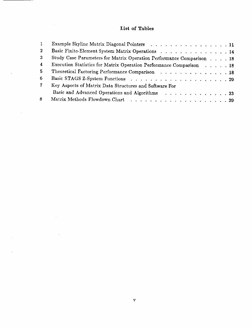
List of Tables
1
2
3
4
5
6
7
Example Skyline Matrix Diagonal Pointers ................ 11
Basic Finite-Element System Matrix Operations .............. 14
Study Case Parameters for Matrix Operation Performance Comparison .... 18
Execution Statistics for Matrix Operation Performance Comparison ..... 18
Theoretical Factoring Performance Comparison .............. 18
Basic STAGS Z-System Functions .................... 29
Key Aspects of Matrix Data Structures and Software For
Basic and Advanced Operations and Algorithms ............. 33
Matrix Methods Flowdown Chart .................... 39

1. Introduction
Forming and manipulating large system matrices are key computational elements in
the solution of large, complicated structural mechanics problems. In the typical case, these
matrices are symmetric and sparsely populated, but of very large order, where the number
of degrees of freedom may range from 100 to 100,000. Much research has been devoted
to the formulation of data storage schemes and computational algorithms that minimize
the computational costs associated with critical matrix manipulations. An example is the
development of equation reordering algorithms to minimize the data storage and number of
arithmetic operations required for the triangular factoring of sparse matrices. The benefits
of such developments have been widespread and have enabled the numerical analysis of
very large and complicated structures to be conducted economically on present computing
machines.
Today, the advancement of Computational Structural Mechanics (CSM) as an effec-
tive engineering tool is still focused on increasing economy, although it considers not only
economy of computational resources but economy of personnel resources as well. Accord-
ingly, new methods such as automatic model error estimation and nonlinear substructuring
are being developed to ease the computational burden on both the analyst and the com-
puter. The CS1V[ Testbed software system (see ref. 1) is intended to aid the development
and implementation of these new methods by providing a common environment for the
development and dissemination of advanced CSM algorithms and procedures. As such,
the Testbed must have features which make it amenable to the incorporation of new, per-
haps unforeseen, numerical operations. The purposes of this document are to identify the
computational matrix algebra capabilities required for the extension of the CSM Testbed's
algorithmic capabilities, and to evaluate the suitability of certain matrix data structures
to accommodate these extensions.
This document is divided into three sections. The first section describes data storage
schemes presently used by the CSM Testbed sparse matrix facilities and similar, skyline
(profile) matrix facilities. The second section contains a discussion of certain features
required for the implementation of particular advanced CSM algorithms, and how these
features might be incorporated into the data storage schemes described previously. The
third section presents recommendations, based on the discussions of the prior sections,
for directing future CSM Testbed development to provide necessary matrix facilities for
advanced algorithm implementation and use.
The discussion presented in the following pages is necessarily limited since to evaluate
all promising matrix data structures and their software would require efforts far in excess
of the scope of the present work. Instead, the discussion is concentrated on the details of
only the Testbed sparse matrix and generic skyline matrix data structures and software.
This narrower focus provides for a deeper examination of these two computational matrix
structures and their applicability to advanced CSM algorithms than would otherwise be
possible. The objective of this document is to lend insight into the matrix structures
discussed and to help explain the process of evaluating alternative matrix data structures
and utilities for subsequent use in the CSM Testbed.
2
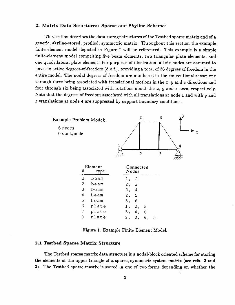
2. Matrix Data Structures: Sparse and Skyline Schemes
This section describes the data storage structures of the Testbed sparse matrix and of a
generic, skyline-stored, profiled, symmetric matrix. Throughout this section the example
finite element model depicted in Figure 1 will be referenced. This example is a simple
finlte-element model comprising five beam elements, two triangular plate elements, and
one quadrilateral plate element. For purposes of illustration, all six nodes are assumed to
have six active degrees-of-freedom (d.o.f.), providing a total of 36 degrees of freedom in the
entire model. The nodal degrees of freedom are numbered in the conventional sense; one
through three being associated with translational motions in the x, y and z directions and
four through six being associated with rotations about the x, y and z axes, respectively.
Note that the degrees of freedom associated with all translations at node 1 and with y and
z translations at node 4 are suppressed by support boundary conditions.
Example Problem Model:
6 nodes
6 d.o.f./nodc //
5
I
2
Element Connected# type Nodes
1 beam i, 2
2 beam 2, 3
3 beam 3, 4
4 beam 2, 5
5 beam 3, 6
6 plate I, 2, 5
7 plate 3, 4, 6
8 plate 2, 3, 6, 5
Figure 1. Example Finite Element Model.
2.1 Testbed Sparse Matrix Structure
The Testbed sparse matrix data structure is a nodal-block oriented scheme for storing
the elements of the upper triangle of a sparse, symmetric system matrix (see refs. 2 and
3). The Testbed sparse matrix is stored in one of two forms depending on whether the
3
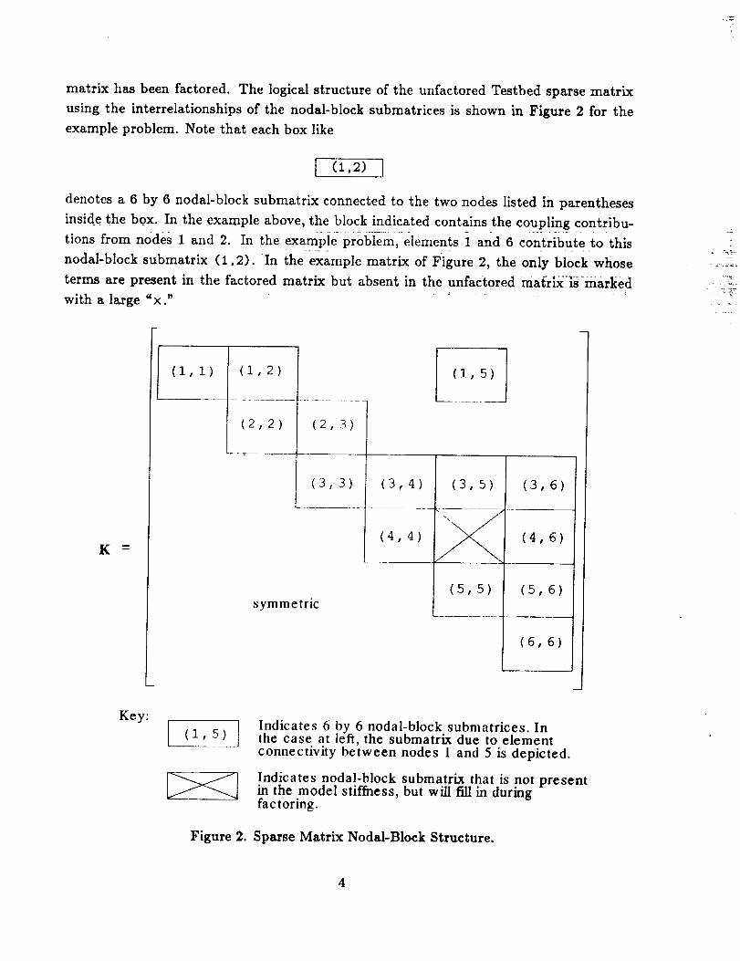
matrix has been factored. The logical structure of the unfactored Testbed sparse matrix
using the interrelationships of the nodal-block submatrices is shown in Figure 2 for the
example problem. Note that each box like
I (1,2) ]
denotes a 6 by 6 nodal-block submatrix connected to the two nodes listed in parentheses
inside the box. In the example above, the block indicated contains the coupling contribu-
tions from nodes 1 and 2. In the example problem, elements i and 6 contribute to this
nodal-block submatrix (1,2). in theexample matrix 0f Figure 2, the only biockwhose
terms are present in the factored matrix but absent in the unfactored matrix:is=marked
with a large "x." _
K ._
(1,1) (1,2)
(2,2)
symmetric
(3,3) (3,4)
(4,4)
(1,5)
(3,5)
(5,5)
(3,6)
(4, 6)
(5,6)
(6,6)
Key:
(1,5)Indicates 6 by 6 nodal-block submatrices. Inthe case at left, the submatrix due to element
connectivity between nodes 1 and 5 is depicted.
Indicates nodal-block submatrix that is not presentin the model stiffness, but will fill in duringfactoring.
Figure 2. Sparse Matrix Nodal-Block Structure.
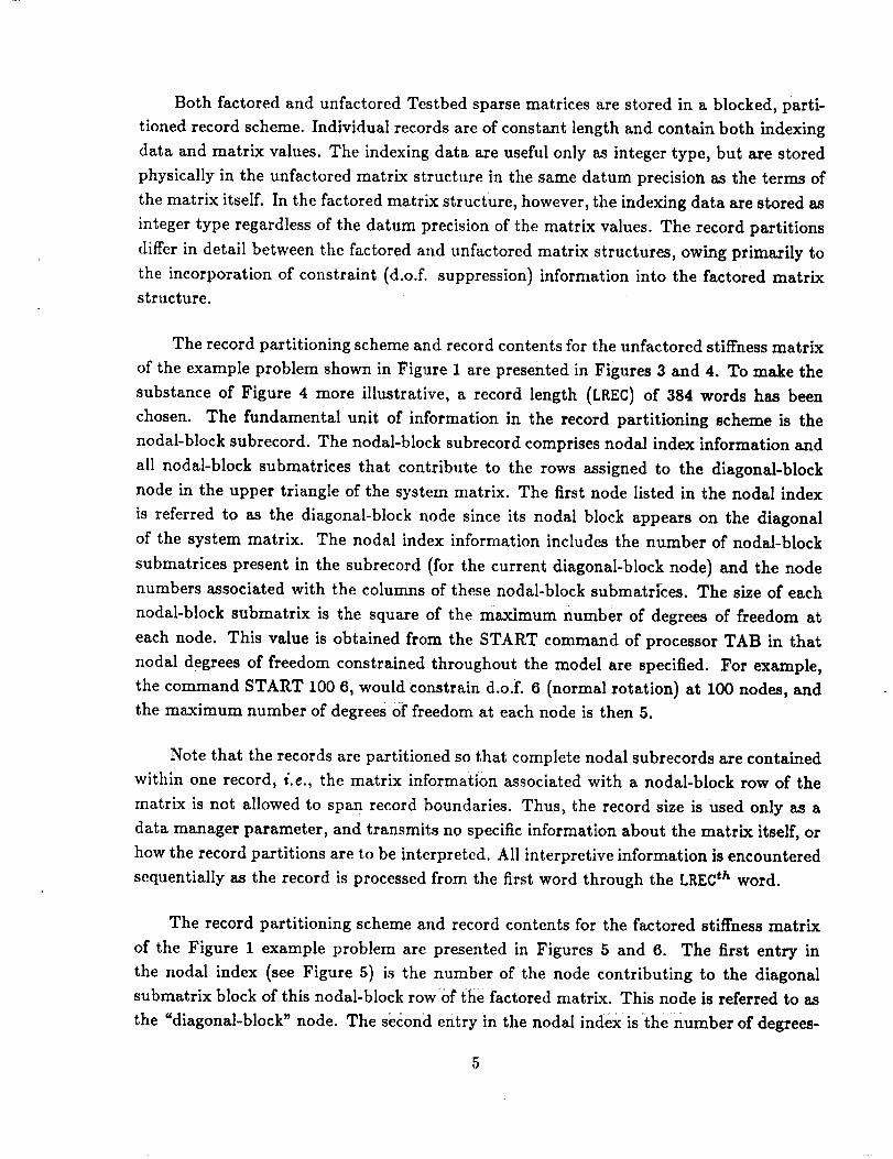
Both factored and unfactored Testbed sparse matrices are stored in a blocked, parti-
tioned record scheme. Individual records are of constant length and contain both indexing
data and matrix values. The indexing data are useful only as integer type, but are stored
physically in the unfactored matrix structure in the same datum precision as the terms of
the matrix itself. In the factored matrix structure, however, the indexing data are stored as
integer type regardless of the datum precision of the matrix values. The record partitions
differ in detail between the factored and unfactored matrix structures, owing primarily to
the incorporation of constraint (d.o.f. suppression) information into the factored matrix
structure.
The record partitioning scheme and record contents for the unfactored stiffness matrix
of the example problem shown in Figure 1 are presented in Figures 3 and 4. To make the
substance of Figure 4 more illustrative, a record length (LREC) of 384 words has been
chosen. The fundamental unit of information in the record partitioning scheme is the
nodal-block subrecord. The nodal-block subrecord comprises nodal index information and
all nodal-block submatrices that contribute to the rows assigned to the diagonal-block
node in the upper triangle of the system matrix. The first node listed in the nodal index
is referred to as the diagonal-block node since its nodal block appears on the diagonal
of the system matrix. The nodal index information includes the number of nodal-block
submatrices present in the subrecord (for the current diagonal-block node) and the node
numbers associated with the columns of these nodal-block submatr|ces. The size of each
nodal-block submatrix is the square of the maximum number of degrees of freedom at
each node. This value is obtained from the START command of processor TAB in that
nodal degrees of freedom constrained throughout the model are specified. For example,
the command START 100 6, would constrain d.o.f. 6 (normal rotation) at 100 nodes, and
the maximum number of degrees of freedom at each node is then 5.
Note that the records are partitioned so that complete nodal subrecords are contained
within one record, i.e., the matrix information associated with a nodal-block row of the
matrix is not allowed to span record boundaries. Thus, the record size is used only as a
data manager parameter, and transmits no specific information about the matrix itself, or
how the record partitions are to be interpretcd. All interpretive information is encountered
sequentially as the record is processed from the first word through the LREC th word.
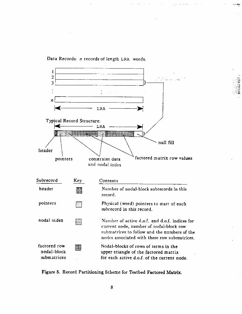
The record partitioning scheme and record contents for the factored stiffness matrix
of the Figure 1 example problem are presented in Figures 5 and 6. The first entry in
the nodal index (see Figure 5) is the number of the node contributing to the diagonal
submatrix block of this nodal-block row of the factored matrix. This node is referred to as
the "diagonal-block" node. The second entry in the nodal index is the number of degrees-
of-freedom active for this diagonal-block node (in the range 1 through 6). Following this
number are the local degree-of-freedom numbers associated with these active degrees-of-
freedom. Each of these local degree-of-freedom numbers are unique and in the range 1
through 6. Following the local degree-of-freedom numbers is the number of off-diagonal
nodal submatrices appearing in this row of the factored matrix. The final entries in the
nodal index are the numbers of the nodes contributing to the off-diagonal nodal-block
submatrices. For purposes of illustration, a record length (LRA) of 384 words was chosen
for the detail of the record contents in Figure 6, and only the first record is shown. The
subscripts of the D-1 and L terms in Figure 6 refer to degree of freedom numbers, assigned
sequentially in groups of six to each node.
Data Records: n records of length LREC words.
l[2
3
I_ LREC _'7
/header
Typical Record Structure: /
_ null fill
nodal index nodal-block submatrices
ll:::::',::::
Subrecord Ke___.._y
header
Contents
number of nodal-block rows in the uppertriangle of the system matrix contained inthis record.
nodal index number of nodes contributing to thenodal-block submatrices in this row and
the numbers of these nodes.
nodal-blocksubmatrices
6 by 6 submatrices of matrix coefficientsin the rows of the upper triangle of thematrix connected to the nodes listed in
the nodal index.
Figure 3, Record Partitioning Scheme for Testbed Unfactored Sparse Matrix.
6
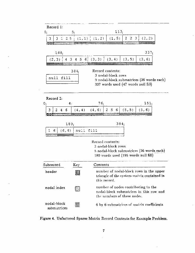
1881 3371
(2,3)I 4 3 4 5 6 i (3,3)I (3,4)I (3,5) (3,6)
3841
null fill
Record contents:
3 nodal-block rows
9 nodal-block submatrices (36 words each)
337 words used (47 words null fill)
Record 2:
01 41 761 1511
1891 384 I
! 6 i (6,6) i null fiil ]
Record contents:
3 nodal-block rows
5 nodal-block submatrices (36 words each)
189 words used (195 words null fill)
Subrecord Key
header :_
nodal index
nodal-block ==
submatrices
Contents
number of nodal-block rows in the upper
triangle of the system matrix contained in
this record.
number of nodes contrib.ting to thenodal-block submatrices in this row and
the n.mbers of these nodes.
6 by 6 submatrices of matrix coefficients
Figure 4. Unfactored Sparse Matrix Record Contents for Example Problem.
7
Data Records: n records oflen_h r, RA words.
1
2
3
,f ILRA _-q
Typical Record Structure: ,/
t--_ LRA __)!!:::i_iii:ii::!i!ii_;4 ..... <.¢;:.-¢';1 ; i i i ;: ; ; ; ; ; ;;,III I1/
f t valuespointers constraint data ac orea matr,x row
and nodal index
Subrecord Key Contents
header
pointers
Number of nodal-block subrecords in this
record.
Physical (word) pointers to start of eachsubrecord in this record.
nodal index
factored rownodal- block
subm atrices
Number of active d.o.f, and d.o.f, indices for
current aode, number of nodal-block row
submatrices to follow and the numbers of the
nodes associated with these row submatrices.
Nodal-blocks of rows of terms in the
upper triangle of the factored matrix
for each active d.o.f, of the current node.
Figure 5. Record Partitioning Scheme for Testbed Factored Matrix.
8

0 41 12|
_ 15811 3 4 5 632 5- I *** D(-41.4) L,4.s) L(4.6, ...1_,z_:;i.i_iii.;i.;:;!!:!.i.;!.!.!i!:iiiiT?-i_i:_i_i:;_i_?...x_,,Z//I,U/.',;-y/x,).'..-..-:..'/.._:._'ff-_ H IIIIllIIIilIIIIIiiiiIlIIIII,,, l,,,
_H-I-H+HH_I i i i i l i]I II IN I I I I I I ; i HIIi i i J ...... ,,H,_ ...... _N, ,,_]]J!H'_" ..........
***** D'1 L L L L 7-_.I•. L 5.10 (6 6) (6 7) • • • (612) (6,25) • • • (6,30)¢ ) , , , ' . ...................• , ; ; ; ill ;i;;;;iii i, J tJ t,,,, *,,,, ,i _[!![!n*n !!! !_L!122_._! !!! !!!1!]I!! _''_!_!_!!h'![! _i! !! !!
".'_///_//_iF/_'_)_//_(_l_j_(_/_a_'_j_//_/:_2.p_.'_'_'_:_'_>_i':_T_; . - i i i i, , I 1 , i ][l I i iii i. / / 1/ It_l ,1_1 IxJI tjJ i.i I_
D('s(s) L(8o) ... L018) * * D(-ol.o) L(o.lo) ... L(oas) * * l/ ' i l ilil ii iiilil,ll, illlll iiill, [ i iii i i, i11 Iiit1[,1111 III Ill'l_llllllllllllll III]
, * • • , D(-l_.n)L(n,12)... L(n.ls)L(n,z)l
1
D(11,1o) L _1o.11) . . • L_IO,18)
".I ',IfI::IllIll: 11'.,/LLII'''_/VIll/tll[l" iI ILLLIIillJLLLLh' I£I LIl LLILLLLII '_''ILlIfLI LI/IIILI :IllIfIll,I
157,
IILLI'A/''"ILILI/AILLIIllI ,I[I]LLIILILLLLIIIUH-_:"_z2222_z:'_Z_A "/-?5d'L//Z&'UZZ
I , -1 L * *6 I 0(]3.13) L¢LU4) • • • L(13,36) 0(14,14) L(14,1_) • • • (_4.36)
k..._./"¢ "171,_11 ...................III1'I1' Ill I I1111 III IlIIIl'i i i i JJJ_ 1 LL.L..Lt J_LL .LILL[i nL_L.tJLI._JLLL LI l i j i i i i i, t i i i i i i i i lI Ill nil IllilllllllllIIlIIIII I_ II_l III' I III III 111 1_. IIl 1J.JLL_ JL |JLL_J.
[ D(]J.Ij) L(15.16) . . . L,,._.._6, * * * DJ,I6) L(I6,1z) . . . L¢16,s6) I
313
D(]l]7)L(1718). . . L(17.36 ) * * * * * D¢/sjs) L(ls,lO). . . L(ls,S6)_;;;_:_j_iii_i_i[_iii_;i`j_i_j_1_!.!!_!!!_!'L_!!!!!_Jt._`[_._!!!'''
fill 384
• - Denotes an unused, subdiagonal entry.
null
Figure 6. Record Contents for Example Problem's Testbed Factored Matrix.
9
As in the unfactored matrix structure, nodal subrecords in the factored matrix are
not allowed to span record boundaries. Unlike the unfactored matrix structure, constraint
data associated with suppression of nodal degrees of freedom are included in the matrix
data records. The factored matrix rows corresponding to suppressed degrees of freedom
are not included in the data. A map is provided at the beginning of the nodal subrecord
to indicate the active degrees of freedom, as an indexed subset (1,...,n) of the degrees
of freedom not constrained on the START card in TAB, for the current diagonal node.
An interesting observation is that the factored matrix data cannot be decoded completely
without additional information about the number of degrees of freedom per node in the
finite element model, and which nodal degrees Of freedom are potentially active. In the
Testbed, this information is obtained from a modeling summary dataset JDF1.BTAB.I.8.
As an aside, one should note that the rather elaborate record partitioning schemes
used for the Testbed matrices are by-products of the architecture of the underlying data
management system (DAL). Three DAL features in particular are responsible for the
original Testbed design choices to place indexing and matrix value data side-by-side in the
data records and to break the matrix storage into fixed-length segments (i.e., records).
These features are:
1) DAL is a singly indexed, hierarchical data manager, so to group data
in logically related sets frequently requires the use of inhomogenous
data records within a single dataset.
2) DAL handles datasets containing fixed-length records only. Different
records in the same dataset cannot have different lengths.
3) DAL is sector (physical disk block) addressable at the finest granular-
ity. Thus, it is required that integer numbers of disk blocks be read
or written through DAL. For practical core memory limitations and
the most efficient use of disk space, the large matrices are blocked
into records that are sized to integer-multiples of the disk block size.
The pertinent observation to be made at this point is that the structure of matrix data is
influenced not only by the structure of the matrix itself (in terms of zero and nonzero coeffi-
cients), but also by the operational characteristics of auxiliary data management software.
Herein lies the most intimate connection between the algebraic and data descriptions of
the system matrix.
10
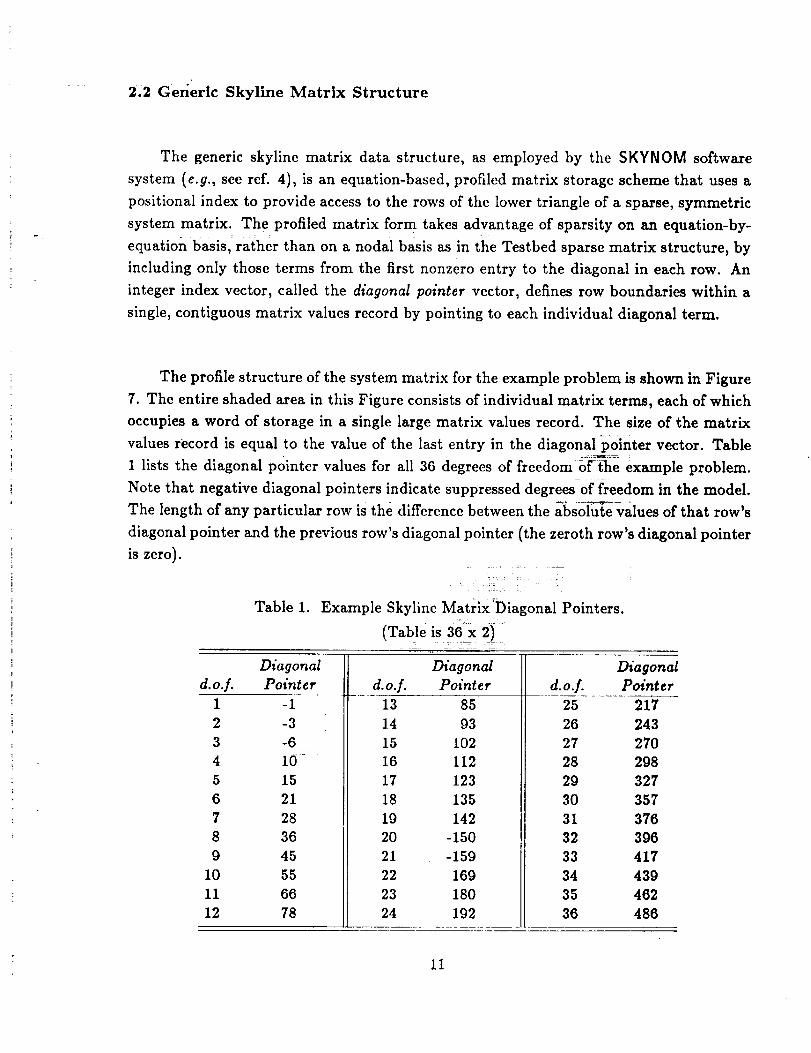
2.2 Generic Skyline Matrix Structure
The generic skyline matrix data structure, as employed by the SKYNOM software
system (e.g., see ref. 4), is an equation-based, profiled matrix storage scheme that uses a
positional index to provide access to the rows of the lower triangle of a sparse, symmetric
system matrix. Theprofiled matrix form takes advantage of sparsity on an equation-by-
equation basis,: rather than on a nodal basis as in the Westbed sparse matrix structure, by
including only those terms from the first nonzero entry to the diagonal in each row. An
integer index vector, called the diagonal pointer vector, defines row boundaries within a
single, contiguous matrix values record by pointing to each individual diagonal term.
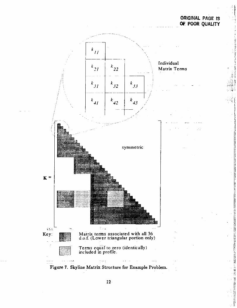
The profile structure of the system matrix for the example problem is shown in Figure
7. The entire shaded area in this Figure consists of individual matrix terms, each of which
occupies a word of storage in a single large matrix values record. The size of the matrix
values record is equal to the value of the last entry in the diagonal pointer vector. Table
1 lists the diagonal pointer values for all 36 degrees of freedom 0f:_l_e example problem.
Note that negative diagonal pointers indicate suppressed degree_offreedom in the model.
The length of any particular row is the difference between the absolute values of that row's
diagonal pointer and the previous row's diagonal pointer (the zeroth row's diagonal pointer
is zero).
Table 1. Example Skyline MatrlxDiagonal Pointers.r
(Table is 36 x 2)
Diagonal
d.o.f. Pointer
1 -1
2 -3
3 -6
4 I0
5 15
6 21
7 28
8 36
9 45
I0 55
11 66
12 78
Diagonal
d.o.f . Pointer
13 85
14 93
15 102
16 112
17 123
18 135
19 142
20 -150
21 -159
22 169
23 180
24 192
Diagonal
d.o.L Pointer
25 217
26 243
27 270
28 298
29 327
30 357
31 376
32 396
33 417
34 439
35 462
36 486
11
ORIGINAL PAGE IS
OF POOR QUALITY
K .,.
kll
k21
k31
k41
k22
k32 k33
k42 k43
/
symme tric
/
'L
Individual
Matrix Terms
2
Key:
\
Matrix terms associated wiih aU 36
d.o.f. (Lower triangular portion only)
Terms equal to zero (identically)included in profde.
Figure 7. Skyline Matrix Structure for Example Problem.
7
12
p;
J_
!?
: 2. ]ili:
r
•J!
Lg
, 15
7t
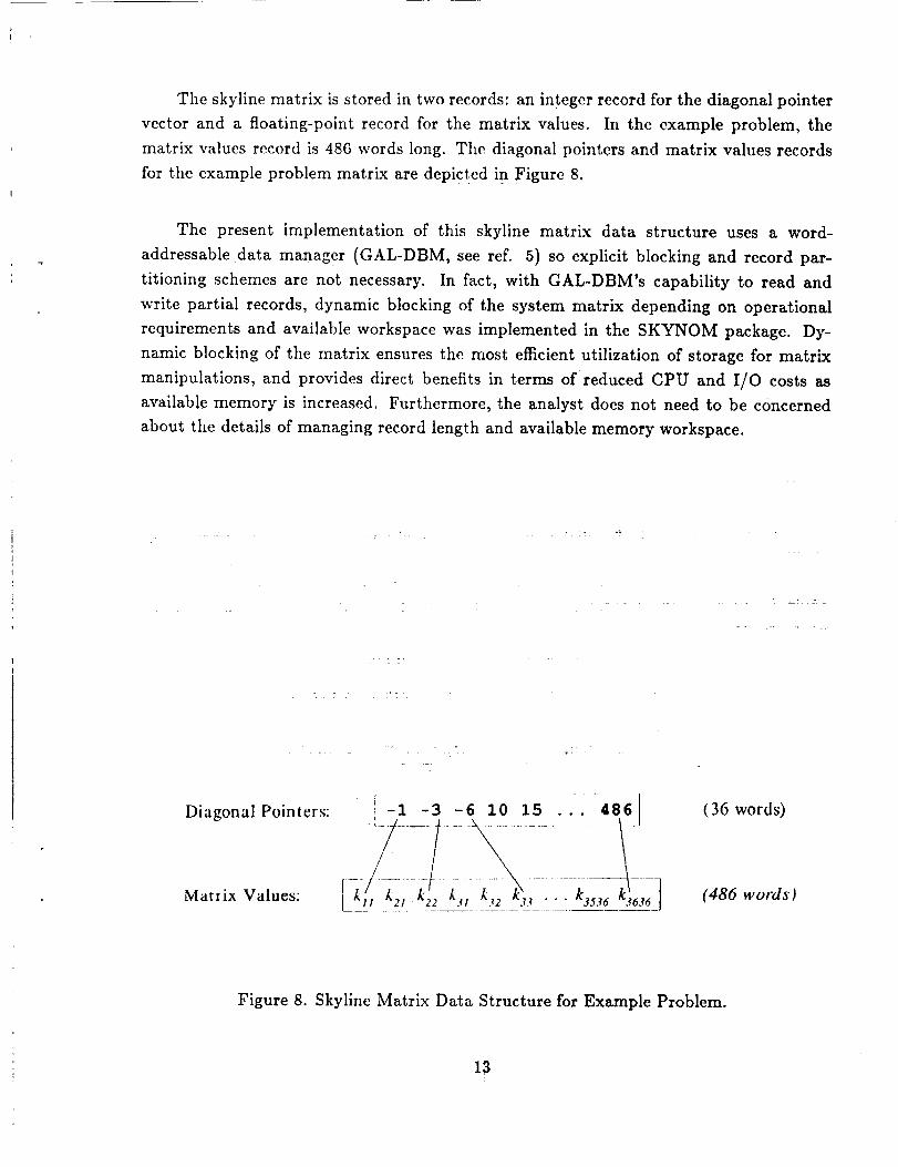
The skyline matrix is stored in two records: an integer record for the diagonal pointer
vector and a floating-point record for the matrix values. In the example problem, the
matrix values record is 486 words long. The diagonal pointcrs and matrix values records
for the example problem matrix are depictcd in Figure 8.
The present implementation of this skyline matrix data structure uses a word-
addressable data manager (GAL-DBM, see ref. 5) so explicit blocking and record par-
titioning schemes are not necessary. In fact, with GAL-DBM's capability to read and
write partial records, dynamic blocking of the system matrix depending on operational
requirements and available workspace was implemented in the SKYNOM package. Dy-
namic blocking of the matrix ensures the most efficient utilization of storage for matrix
manipulations, and provides direct benefits in terms of reduced CPU and I/O costs as
available memory is increased. Furthermore, the analyst does not need to be concerned
about the details of managing record length and available memory workspace.
: : _ 4 =
z
Diagonal Pointers:
Matrix Values:
-1 -3 -6 ...,86i (36 words)
(486 words}
Figure 8. Skyline Matrix Data Structure for Example Problem.
13
3. Algorithm Requirements for Matrix Data Structures
This section explores application-oriented issues of matrix data structures. First, use
of the Testbed sparse and skyline matrix data structures in basic algebraic operations
required by any finite-element analysis is discussed, and the performance of existing soft-
ware for these operations is presented. Second, the applicability of the Testbed sparse
and skyline matrix structures to the execution of advanced algorithms and capabilities
in the Testbed is discussed. This latter section focuses in particular on application Of
the matrix data structures to the use of multipoint constraints, substructuring, advanced
nonlinear algorithms, and p-version finite elements. Most of the discussion in this section
draws on examples from linear formulations of algorithms. Adaptation to nonlinear for-
mulations generally requires only the usual extensions such as iteration procedures and
re-formation of system matrices, and thus simply represents a multiple use of the partic-
ular advanced capabilities. The exceptions to this are the algorithms discussed in Section
3.2.5 for traversing limit and bifurcation points.
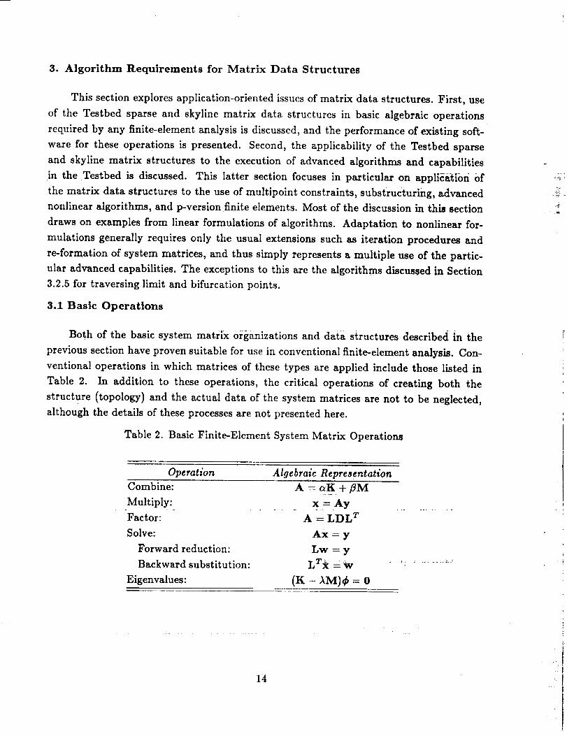
3.1 Basic Operations
Both of the basic system matrix organizations and data structures described in the
previous section have proven suitable for use in conventional finite-element analysis. Con-
ventional operations in which matrices of these types are applied include those listed in
Table 2. In addition to these operations, the critical operations of creating both the
structure (topology) and the actual data of the system matrices are not to be neglected,
although the details of these processes are not presented here.
Table 2. Basic Finite-Element System Matrix Operations
=2
Operation Algebraic Representation
Combine: A = c_K +/3M
Multiply:
Factor:
Solve:
Forward reduction:
Backward substitution:
Eigenvalues:
x -- Ay
A= LDL T
Ax: y
Lw = y
LTx W
(K- AM)_b = 0
14
3.1.1 Software Measured Performance
A primary concern in the utility of any given matrix data structure is the efficiency
with which it can be manipulated by computational routines. Any comparison of diverse
matrix data structures should therefore contain some' measure Of Coinputat[onal efficiency.
However, one must be certain io define carefully the parameters and I_m_ts of validity of
such measures in order to be specific regarding the nature of the comparison.
A simple set of comparisons was made between basic matrix operations in the Testbed
sparse matrix environment and in the $KYNOM skyline matrix environment. The com-
parisons were based on elapsed CPU time and direct I/O requests required for matrix
factoring, matrix-vector multiplication, and matrix equation solution using a previously-
factored matrix. The matrix data for the comparison study were created using the Testbed
software and translated to a skyline format for use with SKYNOM. Three finite element
models were used as a basis for comparison; a 1818 d.o.f, space mast (singly laced, 101-
bay triangular truss), a Coarseiy discretized pinched quarter-cylinder model (square mesh)
with 486 d.o.f.,and a i734 d.o:f, zversion Of the pinched quarter-cylinder model. A variety
of nodal resequencing strategies was employed for the cylinder cases to gain the best fac-
toring performance for each matrix type. In all, five different matrix cases were used for
comparison.
Performance data (CPU time and direct I/O requests) were taken immediately before
and after the issuing of a command to invoke the operation being measured. Since both
the Testbed and SKYNOM are command-driven, some overhead is incurred in command
parsing, and this overhead is included in the measurements. To keep the comparisons on
a common footing, each software package was allowed to use up to 200,000 32-bit words as
a workspace, although no attempt was made to optimize the Testbed sparse matrix record
length with respect to workspace usage. In addition, one should note that SKYNOM's
automatic allocation of workspaceand dynamic matrix blocking requires measured CPU
and I/O resources not required by the explicitly blocked sparse matrix. All calculations
were made in double (64'bit) precision. All executions were made in a single job stream
on a VAX-ll/785 computer system to eliminate as much machine-environment variability
as possible.
15
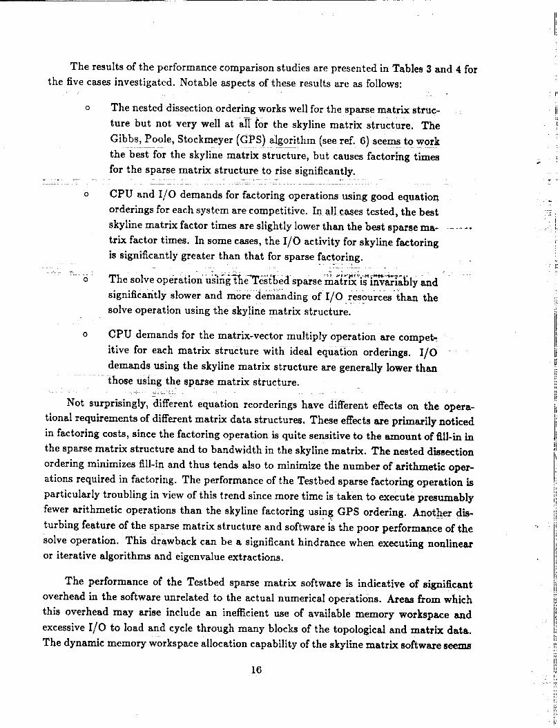
The resultsof the performancecomparisonstudies are presentedin Tables3 and 4 forthe five casesinvestigated. Notable aspectsof theseresults are asfollows:
o The nested dissection ordering works well for the sparse matrix stru¢- :
ture but not very Well at all for the skyline matrix structure. TEe
Gibbs, Poole, Stockmeyer (GPS) algorithm (see ref. 6) seems to wor k
the best for the skyline matrix structure, but causes factoring times
for the sparse matrix structure to rise significantly.
o CPU and I/O demands for factoring operations using good equation
orderings for each system are competitive. In all cases tested, the best
skyline matrix factor times are slightly lower than the best sparse ma-
trix factor times. In some cases, the I/O activity forskyline factoring
is significantly greater than that for sparse factoring.
o The solve operation using t_eTest_ed sparsematr[x_isinv_ia_ly and
significantly slower and more demanding of I/O resources than the
solve operation using the skyline matrix structure.
o CPU demands for the matrix-vector multiply operation are compet-
itive for each matrix structure with ideal equation orderings. I]O
demands using the skyline matrix structure are generally lower than
" - those Us|ng the sparse matrix structure.
Not surprisingly, different equation reorderings have different effects on the opera-
tional requirements of different matrix data structures. These effects are primarily noticed
in factoring costs, since the factoring operation is quite sensitive to the amount of fill-in in
the sparse matrix structure and to bandwidth in the skyline matrix. The nested dissection
ordering minimizes fill-in and thus tends also to minimize the number of arithmetic oper-
ations required in factoring. The performance of the Testbed sparse factoring operation is
particularly troubling in view of this trend since more t|me is taken to execute presumably
fewer arithmetic operations than the skyline factoring using GP$ ordering. Another dis-
turblng feature of the sparse matrix structure and software is the poor performance of the
solve operation. This drawback can be a significant hindrance when executing nonlinear
or iterative algorithms and eigenvalue extractions.
The performance of the Testbed sparse matrix software is indicative of significant
overhead in the software unrelated to the actual numerical operations: Areas from which
this overhead may arise include an inefficient use of available memory workspace and
excessive I/O to load and cycle through many blocks of the topological and matrix data.
The dynamic memory w0rkspace allocation capability of the skyline matrix software seems
16
!.
I:
1i
it
J_;i
i`¸¸ i_
• i_̧
to provide an advantage primarily in reduction of I/O requests for solve and multiply
operations. In these cases, SKYNOM is able to fit more of the matrix into the workspace
at once, causing fewer I/O requests but more words transferred per request. On machines
where I/O requests dominate I/O costs, this savings can be significant.
Making the Testbed software use available memory effectively is difficult since user
intervention is required to modulate the dataset record sizes of KMAP, AMAP, K and INV
dat_ets (see ref. 7). For fixed-memory applications, even optimal sizing of these datasets'
records would result in a loss of efficiency in the solve operation since the maximum size of
the factored matrix records is determined in the factoring process and the solve operation
is processed on a record-by-record basis. Thus, basic inefficiencies are incurred by the use
of the fixed-length, explicitly blocked matrix data structure. :
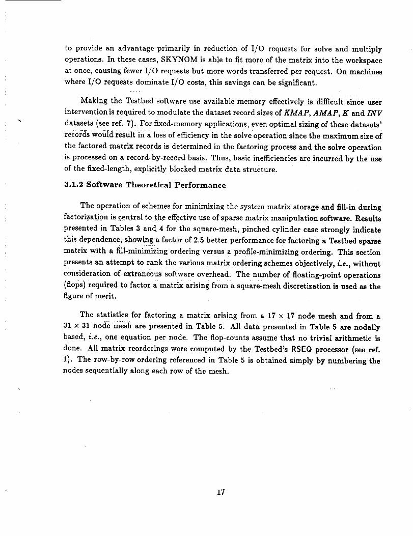
3.1.2 Software Theoretical Performance
The operation of schemes for minimizing the system matrix storage and fill-in during
factor!zation iscentral to: the effective use of sparse matrix manipulation software. Results
presented in Tables 3 and 4 for the square-mesh, pinched cylinder case strongly indicate
this dependence, showing a factor of 2.5 better performance for factoring a Testbed sparse
matrix with a fill-minimizing ordering versus a profile-minimizing ordering. This section
presents an attempt to rank the various matrix ordering schemes objectively, i.e., without
consideration of extraneous software overhead. The number of floating-point operations
(flops) required to factor a matrix arising from a square-mesh discretization is used as the
figure of merit.
The statistics for factoring a matrix arising from a 17 × 17 node mesh and from a
31 x 31 node mesh are presented in Table 5. All data presented in Table 5 are nodally
based, i.e., one equation per node. The flop'counts assume that no trivial arithmetic is
done. All matrix reorderings were computed by the Testbed's RSF:Q processor (see ref.
1). The row-by-row ordering referenced in Table 5 is obtained simply by numbering the
nodes sequentially along each row of the mesh.
17
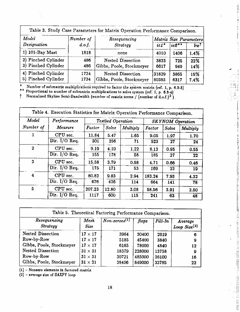
Table 3. Study Case Parameters for Matrix Operation Performance Comparison.
Matriz Size ParametersModel
Designation
I) 101-Bay Mast
2) Pinched Cylinder
3) Pinched Cylinder
4) Pinched Cylinder
5) Pinched Cylinder
Number of
d.oJ.
1818
486
486
1734
1734
Resequencing
Strategy
none
Nested Dissection
Gibbs, Poole, Stockmeyer
Nested Dissection
Gibbs, Poole, Stockmeyer
it1 *
4010
3833
6617
31829
80385
ie_** bwt
1406 1.4%
725 ' 22%
949 14%
3865 15%
6317 7.4%
* Number of submatrlx multiplications required to factor the System matrb (ref. 1, p. 6.S-3)** Proportional to number of submatrix multiplications to solve system (ref.- i, p. 6.3-4) "
t Normalized Skyline Semi-Bandwidth (number of matrix terms / (number of d.o.f.) 2 )
ii
Table 4. Execution Statistics for Matrix Operation Performance Comparison.
Model
Number of
Performance
Measure
CPU sec.
Dir. I/O Req.
CPU sec.
Dir. I/O Req.
Testbed Operation
Factor
11.84
301
9.19
155
Solve
5.47
256
4.10
178
Multiply
1.65
71
1.22
58
SKYNOM Operation
Factor
9.05
523
8.13
185
3 CPU sec. 15.58 3.79 0.98 4.71
Dir. I/O Req. 175 171 53 169
4 CPU sec. 80.82 9.83 2.94 183.24
Dir. I/O Req. 676 436 114 664
5 CPU sec. 207.23 12.80 3.08 58.56
Dir. I/O Req. 1117 600 115 241
Solve Multiply
1.97 1.70
27 24
0.95 0.55
27 22
0.66 0.46
23 19
7.93 4.32
141 78
3.91 2.50
63 48
< ::_ i..... i
J_
r
i.
i:
Table 5. Theoretical Factoring Performance Comparison.
-Resequ encing
Strategy
Nested Dissection
Row-by-Row
Gibbs, Poole, StockmeyerNested Dissection
Row-by-Row
Gibbs, Poole, Stockmeyer
Mesh
Size
17 x 17
17 x 17
17 x 17
31 × 31
31 x 31
31 x 31
Non-zeroes(1)
3964
5185
6185
18379
30721
38406
flops
30400
45400
78000
228000
485000
849000
Fill-In
2619
3840
4840
13758
26100
33785
(I)- Nonzeroelementsinfactoredmatrix
(2)- averagesizeofSAXPY loop
Average
Loop Size( z )
6
9
12
9
16
22
18
!:
l,
. Ji
J_
From the data presented in Table 5, one can readily see that the nested dissection or-
dering theoretically requires many fewer arithmetic operations for factoring than either the
natural, row-by-row ordering or the Gibbs, Poole, Stockmeyer ordering. Also, the ratio of
flops between the nested dissection and Gibbs, Poole, Stockmeyer cases is reasonably close
to the ratio of CPU times for these two cases in Table 4. One should note, however, that
the flop-counts for the row-by-row or Gibbs, Poole, Stoekmeyer orderings do not correlate
with the CPU time statistics when comparing Testbed and SKYNOMperformance. In
particular, the Testbed factoring on the 17 × 17 node mesh with nested dissection ordering
exhibits a computational average rate of approximately '376 nodal flops per CPU second
whereas the SKYNOM factoring of the same matrix ordered according to the Gibbs, Poole,
Stockmeyer algorithm exhibits a computational rate of approximately 775 nodal flops per
second (discounting trivial arithmetic).
3.2 Advanced Operations
: virtually all advanced matrix operations Can be described as a suitable combination
of the more elementary operations listed in Table 2. Indeed, this is how the algebraic
descriptions of advanced algorithms are evolved. Two factors impede the adoption of an
analogous numerical approach, however. These factors are the consideration of efficiency
in numerical operations and the restrictions arising from matrix data structures.
Considerations of numerical efficiency often drive algorithms deep into code, since
that is where computational efficiency is most obtainable. Thus, a question arising for
advanced algorithm development is:
o "How easy is the modification of the basic operations' code to accom-
modate necessary new operations?"
As the operations' code is constructed to operate using a particular structure of matrix
data, this first question is directly linked to another:
o "How amenable is the matrix data structure to the new operation's
requirements?"
The answers to these related questions, with respect to the Testbed sparse and generic
skyline matrix software, are the subject of the following sections. The following discussion
explores these questions in light of the requirements of specific near-term Testbed advanced
algorithms and capabilities including general constraints, substructuring, advanced Riks
procedures, equivalence transformation procedures, and p-version finite elements.
19
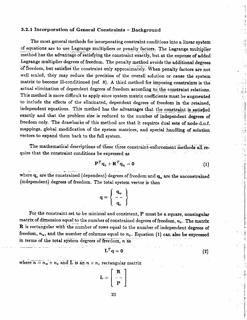
3.2.1 Incorporation of General Constraints Background
The most general methods for incorporating constraint conditions into a linear system
of equations are to use Lagrange multipliers or penalty factors. The Lagrange multiplier
method has the advantage _satisfying the constraint exactly, but at the expense of added
Lagrange multiplier degrees of freedom. The penalty method avoids the additional degrees
of freedom, but satisfies the constraint only approximately. When penalty factors are not
well scaled, they may reduce the precision of the overall solution or cause the system
matrix to become ill-conditioned (ref. 8). A third method for imposing constraints is the
actual elimination of dependent degrees of freedom according to the constraint relations.
This method is more dli_icult to apply since system matrix coefficients must be augmented
to include the effects of the eliminated, dependent degrees of freedom in the retained,
independent equations. This method has the advantages that t heconstraint _satisfied
exactly and that the problem size is reduced to the number of independent degrees of
freedom only. The drawbacks of this method are that it requires dual sets of node-d.o.f.
mappings, global modification of the system matrices, and special handling of solution
vectors to expand them back to the full system.
The mathematical descriptions of these three constraln_;-enforcement'naethods all re-
quire that the constraint conditions be expressed as
pTqc + RTqu : 0 (1)
where qc are the constrained (dependent) degrees of freedom and qu are the unconstrained
(independent) degrees of freedom. The total system vector is then
{qu}q _ m --
qc
For the constraint set to be minimal and consistent, P must be a square, nonslngular
matrix of dimension equal to the number of constrained degrees of freedom, nc. The matrix
R is rectangular with the number of rows equal to the number of independent degrees of
freedom, nu, and the number of Columns equal to nc. Equation (1) can also be expressed
in terms of the total system degrees o__m.--n :_: ...........................
:.: T - .... : ....
where-n - nu ÷ nc and _L is an n × n_ rectangular matrix
LTq=0 (2)
P
2O
=! [
L
[=
t:
il
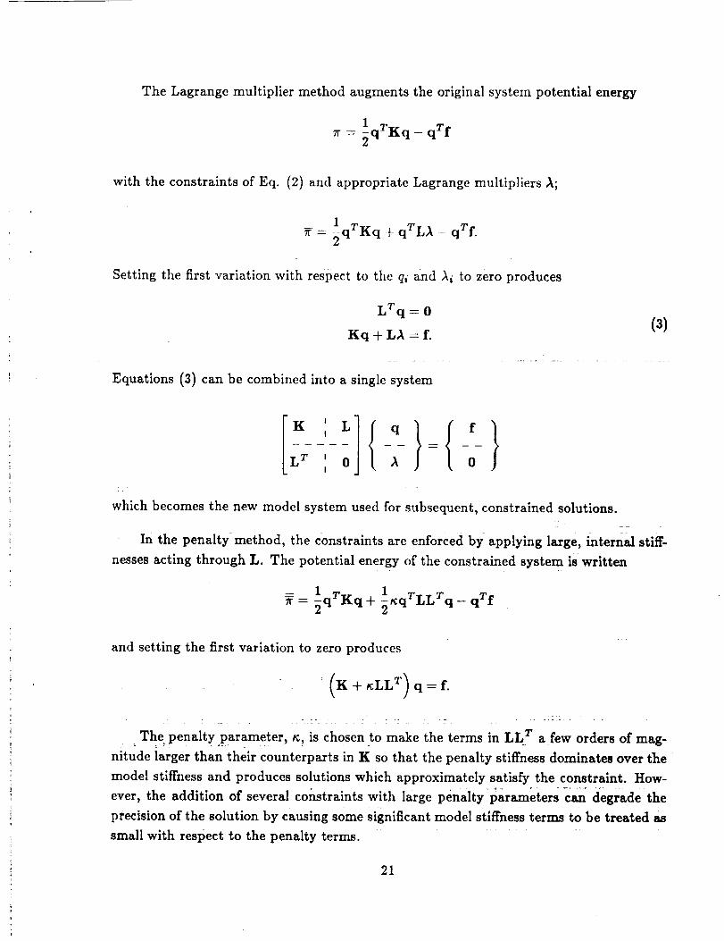
The Lagrange multiplier method augments the original system potential energy
r = lqTKq-- qTf2
with the constraints of Eq. (2) and appropriate Lagrange multipliers A;
= 1-qTKq + qTLA - qTf.2
Setting the first variation with respect to the q_ and A_ to zero produces
LTq -----0
Kq + LA = f.
Equations (3) can be combined into a single system
(3)
s L
K I
L T I 0I
(q/{'/A 0
which becomes the new model system used for subsequent, constrained solutions.
In the penalty method, the constraints are enforced by applying large, internal stiff-
nesses acting through L. The potential energy of the constrained system is written
and setting the first variation to zero produces
K + gLL T) q - f.
The penalty parameter, t¢, is chosen to make the terms in LL T a few orders of mag-
nitude larger than their counterparts in K so that the penalty stiffness dominates over the
model stiffness and produces solutions which approximately satisfy the constraint. How-
ever, the addition of several constraints with large penalty parameters can degrade the
precision of the solution by causing some significant model stiffness terms to be treated as
small with respect to the penalty terms.
21
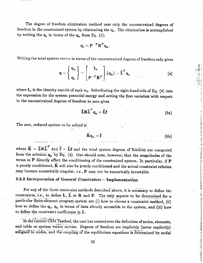
The degree of freedom elimination method uses only the unconstrained degrees of
freedom in the constrained system by eliminating the qc- The elimination is accomplished
by writing the qc in terms of the qu from Eq. (1);
qc = p-TRTqu"
Writing the total system vector in terms of the unconstrained degrees of freedom only gives
EIuq : p_rR Tqc
{qu} _T: q_ (4)
where Iu is the identity matrix of rank nu. Substituting the right-hand side of Eq. (4) into
the expression for the system potentiaienergy andsetting the first variation with respect
to the unconstrained degrees of freedom to zero gives
f Kf,Tq. = f,f (5a)
The new, reduced system to be solved is
Kq. = i"
where R = LKL T and f : _,f and the total system degrees oft'reedom are computed
from-tHe solut_on=qu_by Eq: (4). One should note, however, that the magnitudes of the
terms in P'dlrectiy affeci the conditioning of the constrained system. In particular, if P
is poorly conditioned, K will also be poorly conditioned and the actual constraint relation
may become numericaUy singular, i.e., P m_y not be numerically invertable.
(bb)
3.2.2 Incorporation of General Constraints - Implementation
For any of the three constraint methods described =above, it is necessary to define the
constraints, i.e., to define L, L or R andP. The only _pects to be deteim!ned for a
particular _nite-element program system are (i) how to choose a constraint method, (ii)
how to define the qc, qu in terms of data already accessible to the system, and (iii) how
to define the constraint c0efficidnts ip L. :: °" : _::
7 .... : = ?:
.... l_n the-curre'nt_ CS_MTestbed, the user has control over the definition of nodes, elements,
and:table or system vector-entries. Degrees of freedom are implicitly (never explicitly)
ass g'nh d nodhs.ana ihe_c0upiing of the equilibrium equations is=determined by nodal
22
connectivity rather than degreeof freedom connectivity. With theseoperational features,the constraint data must be defined in nodal terms.
The nodal-block organization of the Testbed sparse matrix requires that constraint
data be associated with nodes. Accordingly, Lagrange multipliers must be associated with
a "dummy" node, i.e., a node with no structural model degree of freedom. The Lagrange
multiplier method, as implemented in SPAR Level 13A (ref. 9), required the use of the
experimental element facility to define a stiffness matrix format containing the L matrix
for a constraint element connected to m + 1 nodes, where m is the number of nodes having
degrees of freedom corresponding to nonzero terms in L. The number of constraints that
could be associated with a single dummy node would be up to the number of active degrees
of freedom per node. Node-to-node constraints are the only kind of constraints that are
implemented easily in this system.
The penalty method could be readily applied to the Testbed sparse matrix in the
same manner as the Lagrange multipliers were incorporated but without the necessity for
dummy nodes. In this case, a penalty element matrix could be defined to be assembled
directly with all other structural elements.
The degree of freedom elimination scheme is difficult to apply to the Testbed sparse
matrix structure. The implementation would most likely assemble the portions of the com-
plete matrix associated with independent and dependent degrees of freedom in separate
nodal-block matrices and combine them appropriately to produce the global, reduced sys-
tem matrix K. The topology analysis must also account for the connectivity of the nodes
of the dependent degrees of freedom in consideration of nodal connectivity of each con-
stituent independent degree of freedom. Structures analogous to the JDF1.BTAB.1.8 and
CON..ncon datasets (see ref. 7) are required for use with the reduced system since system
vectors are shortened and constraint data are not as straightforward as simple degree of
freedom suppression. Special consideration is needed for the flagging of constrained degrees
of freedom that have been eliminated, since no constraint types in addition to Uprescribed
zero" and _prescribed nonzero" can be accommodated in the structure of GON..ncon and
the constraint relations do not fit into the structure of an APPL.MOTI system vector.
Incorporation of constraints into the skyline matrix structure would be more straight-
forward than incorporation into the Testbed sparse matrix structure simply because the
skyline structure is based on degrees of freedom rather than on nodes. Furthermore,
since no integrated finite-element software analogous to the Testbed has been built up
around the generic skyline matrix package, no potential conflicts exist between d.o.f.-by-
d.o.f, augmentation or reduction of the equation system and auxiliary system data like
the JDFI.BTAB dataset used by the Testbed software. Also, the pointer vector to matrix
23
diagonal terms (referred to asa diagonal-pointer vector) provides a single, minimally sized
map of the contents of the single matrix values record, making access to any portion of
the skyline-stored matrix straightforward. However, if bandwidth minimization schemes
are employed, equivalence constraint information must be taken into account in the deter-
mination of degree of freedom connectivity in order to preserve efficiency in the factoring
of the constrained matrix.
Lagrangian constraints wou!dbe: !mplemented into the sky!!ne matr'txstructure !n a
manner:::_....analogous to the Testbed spars e matrix implementat!0n- _ a special ::constraint
element." The constraint element in thls case would have a minimum of three degrees
of...........freedom, rather than three associate d node s (18 degrees of freedom), and wou!d be
included directly in the topology analysis and matrix assembly processes. Incorporation of
penalty constraints in the skyline matr_ s_tructure isals 0 quite straightforward and would
be accomplished through the device of a Constraint element _formed by a special'purpose
processor. This approach would follOW a new development implemented into the STAGS
program (see refs. 10 and 11) which useci an augmented Lagrangian _api_roach to define
multi-point constraints, eliminating past problems with equation ordering and otherwi_
unconnected structures.
The degree of freedom elimination procedurefor the skyiinematrix data structure is
almost as difficultas=for the Westbed sparse matrix, although none of the incompatibilities
wit_: other mod_-d_ecor:_s:are _present: _structure_is_sl-mp_fleci th-rr0ug_e use
of the diagonal: po|nter vector, which is defined by only the 10Test'referenced degree of
freedom in any equati0-n, rather than lJy all connectedn0des:=(or degrees of freedom).
In the skyline format as in_ the Te_t:b_e-d: sparse format; matr_ "coefficients would most
probabiy best be :caiculatecl_0n a term-by-term basis and:assembled into a- reduced-order
system matrix.
3.2.3 Substructuring Operations - Background
Wl_e use of substructures -pro:m:ises __reat :payoff in reducing the size of very large
analysis problems. In global-local analysis, substructuring is a crucial procedure to remove
slowly varying, global phenomena from a h!ghly detailed, perhaps nonlinear, local model
without ad hoc assumptions regarding local boundary conditions. :
The procedure used in substructuring is to express the degrees of freedom associated
with some subregion of the domain, called the interior domain, ]n terms of the degrees of
freedom in some other subregion of the d0_ain, called the boundary _bma|h__l_0:_c_)mplish
24
i.!
t
i.!
i
! =
this, the following partition is used for the system equilibrium equation:
[ K T Kbb qb fb
(6)
The interior degrees of freedom, qi, are elim!nated to produce the equilibrium equation in
terms of the boundary degrees of freedom:
(Kbb -- KTK_IKib) qb = fb - KTK_Xfi
with
qi = K_ I (fi - Kibqb)
Note that when a diagonal-scale factoring of the interior matrix Kii is used (Kil =
LDLT);
T -1KibKii Kib = wTD-1w
where
L TW = Kib
The computation of w requires only a single-pass reduction and can save approximately
half the cost of a full, forward-reduction and back-substitution solution procedure.
For multiple substructures, each interior domain is expressed in terms of a set of
retained boundary degrees of freedom, whose matrix coefficients are assembled into the
final retained equation. In the nonlinear case, degrees of freedom associated with the
nonlinear domain are also included in the retained system, which is then solved using
nonlinear procedures.
An alternative approach to substructuring, and that taken in the substructuring capa-
bility presently implemented in the CSM Testbed, is to express the motion of the boundary
as a linear combination of suitable boundary functions, by. This approach is from SPAR
Level 13A (ref. 9). These boundary functions are the total displacement pattern of the in-
terior and boundary degrees of freedom under a unit-imposed displacement at exactly one
boundary degree of freedom, with all others suppressed. Thus, the number of boundary
functions is equal to the number of boundary nodes times the number of degrees of freedom
per node. The by also contain contributions to the motions of the interior domain degrees
25
of freedom. The remainder of the interior motions are described through a user-defined
set of interior displacement functions, qY" The displacement of the entire domain is
nb nl
q = Z bjxj + _ qkYk (8)
j=l k----1
where nb are the boundary degrees of freedom, ni are the interior displacement functions,
and the x i and Yk are the amplitudes of the jth boundary function and k th interior dis-
placement function, respectively. Denoting the matrix whose columns are the bj as B and
the matrix whose columns are the qk as Q, the equiiibriumEq. (6) can be rewritten as
BTKB
0
o
QTKQ
(o)
The decoupled system of Eq. (9) can be solved for the amplitudes of the boundary functions
and the interior displacements. For the static problem, an exact solution is obtained when
the Q contains an interior displacement vector due to is with fb = 0. Otherwise, an
approximate solution will result in the interior domain causing the global solution also to
be only approximate.
3.2.4 Substructurlng Operations - Implementation
The Testbed sparse matrix substructuring scheme requires the following calculations:
1) Form the full system matrix K.
2) Factor K with all boundary degrees of freedom prescribed and solve
for the n b boundary functions b i.
3) Solve for the interior displacement functions qk.
4)NT N
Calculate BTKB and Q KQ and store as full, lower-triangular
matrices.
5) Factor BTKB and QTKQ and solve Eq. (9).
6) Expand the solution vectors x and y into full system solution vectors
q = Bx + Qy.
The steps indicated above are implemented in the CSM Testbed for dynamic analysis
through several processors: K, INV. SSOk. AUS/SSPREP. AUS/SSM. AUS/SSK. SYN.
26
STRP. and SSBT. At present, the detailed structure of the matrices generated by SYN is
not known. Neither is the compatibility of SYN matrices with INV and AUS/PROD known.
One characteristic that is documented is that SYN must work with models using no less
than 6 degrees of freedom per node. The only Testbed substructuring procedure presently
fully documented for use is for substructured vibration eigenvalue analysis.
Management of substructures in the Testbed is accomplished by segregating individual
substructures into separate data libraries. Thus, confusion over domain-specific tabular
data (e.g., JDF1, ALTR, JLOC, JREF and CON) is avoided in operations using "full
model" processors like INY and $$0[. for individual substructure systems. Thus each
substructure model can retain its own local system matrices.
Aside from the definition of substructure interior and boundary domains, two unique
capabilities are required to implement a partitioned substructuring _cheme effectively.
These are (a) a capability to extract or construct the boundary coupling matrix K_b and
(b) the upper-triangular matrix solution procedure to determine w.
The Kib matrix can be formed directly from the boundary functions matrix B by
extracting only those terms corresponding to interior degrees of freedom, but computation
of the B matrix requires nb complete solutions (forward and backward substitutions).
Computation of the w matrix requires half the work, but assumes the coefficients of K_b
are available in a vector-block form. The complete Kib is, of course, already available in
the assembled system K, but extraction from that structure would be difficult, especially
using the Testbed sparse matrix data structure. A more effective approach might be to
use a substructure assembler processor that would assemble the K;_, Kbb and K_b directly
from constituent element matrices. In this way, bandwidth minimization techniques could
be applied independently to the diagonal submatrices K/_ and Kbb,
A very general matrix assembly routine would also aid in forming the Schur comple-
ment
(Kbb- KTK_iK,b)= (Kbb--wTD-Iw)
since the matrix product will, in general, be full while the I_bb may be sparse. At present,
no capability exists for combining Testbed sparse matrices with full, square matrices or
matrices of differing topologies.
The skyline matrix organization offers little formulative advantage over the Testbed
sparse matrix system if an approach similar to that taken presently in the Testbed is
followed, i.e., the boundary-function matrix reduction is used. If, on the other hand,
a partitioning scheme were to be used, the picture changes slightly since significantly
27
more control over the submatrix assembly process could be designed into a needed skyline
matrix assembler. Also, the triangular-matrix solution operation is presently available for
the skyline matrix structure.
3.2.5 Advanced Solution Algorithms -Requirements
Advanced nonlinear solution algorithms, like the Riks (see refs. 12 and 13) and
Crisfield (see ref. 14) methods, generally require some special handling of system ma-
trices near limit and bifurcation points. The equivalence transformation algorithm (see
refs. 15 and 16) has been developed to select appropriate soiut]0n paths beyond imminent
bifurcations. Many of these algorithms treat the critical points using a reduced system
calculated by transformation of the full system.
While the requirements of each nonlinear solution algorithm differ in detail to a great
extent, common elements can be extracted and used to formulate a generic toolkit of neces-
sary linear algebraic operations. Such an approach has been taken in the STAGS program
wherein a group of utilities, called the Z-system (see ref. 11), has been created and is
presently being used to provide the computational functionality necessary for executing
the enhanced Riks and equivalence transformation algorithms. The functionality of the
Z-system encompasses the basic finite-element operations enumerated in Table 2 plus addi-
tional operations to (a) suppress and enable individual degrees of freedom dynamically, (b)
extract values of degrees of freedom, (c) assemble system vectors at the element level, and
(d) compute matrix-vector products on an element-by-element basis. The basic Z-system
functionality is presented in Table 6. Many functions are simply vector manipulations and,
as such, do not depend on the architecture of system matrix software or data structures.
3.2.6 Advanced Solution Algorithms - Implementation
Emulation of the Z-system functionality using the CSM Testbed sparse matrix struc-
ture requires minimal enhancement, providing the combination of system matrices is re-
stricted to matrices of identical structure, and software is constructed or extracted to
modify the packed-word entries in the dataset CON..ncon outside of the processor TAB.
A capability for vector assembly is necessary in the Testbed, as is one for element-by-
element matrix-vector multiplication (function I_XVEC in Table 6). Based on experience
with STAGS, these two operations can save significant storage and I/O costs during non-
linear iterations.
28
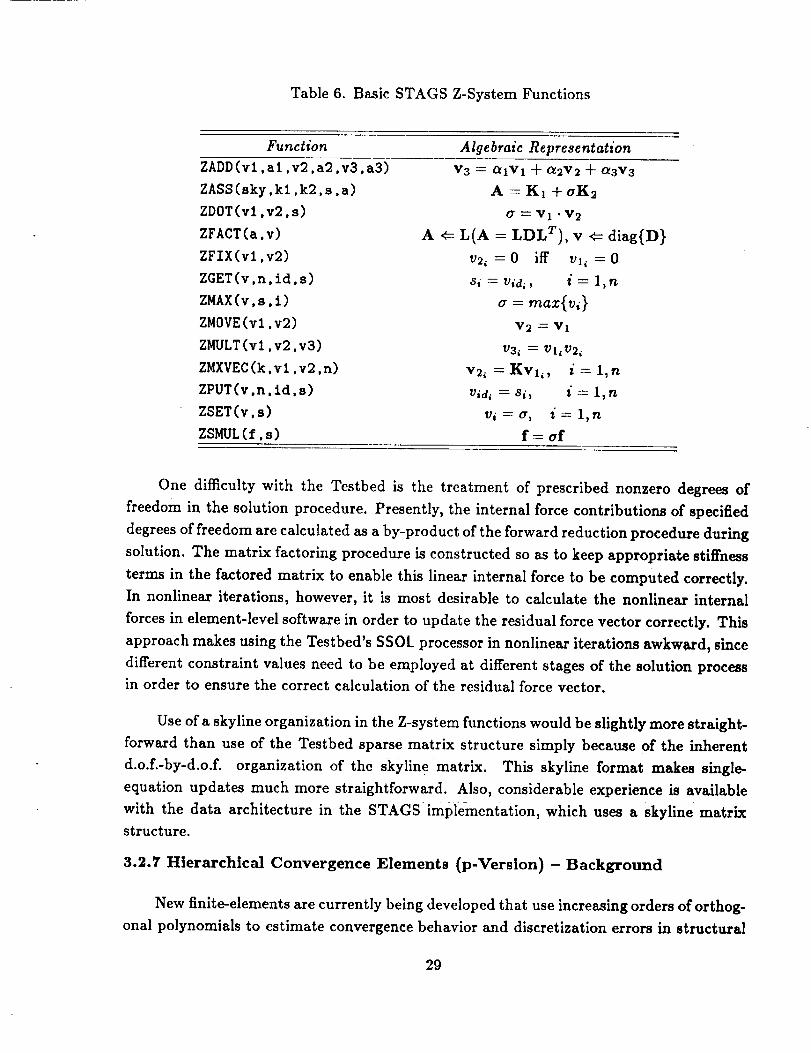
Table 6. Basic STAGS Z-System Functions
Function Algebraic Representation
ZADD(vl,al,v2,a2,v3,a3)
ZASS(sky,kl,k2,s,a)
ZDOT(vl,v2,s)
ZFACT(a,v)
ZFIX(vl,v2)
ZGET(v,n,id,s)
ZMAX(v,s,i)
ZMOVE(vl.v2)
ZMULT(vl.v2.v3)
ZMXVEC(k,vl.v2,n)
ZPUT(v.n,id,s)
ZSET(v,s)
ZSMUL(f,s)
V 3 _ _iVl + OL2V2 + OL3V3
A =Kl +aK2
G -----Vl'V 2
A _ L(A = LDLT), v ¢= diag{V}
v_, = O if[ vl, =0
,_i = rid;, i = 1, n
a = rnax{vi}
V 2 = V I
U3_ = UIIU21
V2_ =KvI_, i= l_n
Vidl = 8i_ i _ 1, n
vi = a, i----1,n
f: af
One difficulty with the Testbed is the treatment of prescribed nonzero degrees of
freedom in the solution procedure. Presently, the internal force contributions of specified
degrees of freedom are calculated as a by-product of the forward reduction procedure during
solution. The matrix factoring procedure is constructed so as to keep appropriate stiffness
terms in the factored matrix to enable this linear internal force to be computed correctly.
In nonlinear iterations, however, it is most desirable to calculate the nonlinear internal
forces in element-level software in order to update the residual force vector correctly. This
approach makes using the Testbed's SSOL processor in nonlinear iterations awkward, since
different constraint values need to be employed at different stages of the solution process
in order to ensure the correct calculation of the residual force vector.
Use of a skyline organization in the Z-system functions would be slightly more straight-
forward than use of the Testbed sparse matrix structure simply because of the inherent
d.o.f.-by-d.o.f, organization of the skyline matrix. This skyline format makes single-
equation updates much more straightforward. Also, considerable experience is available
with the data architecture in the STAGS implementation, which uses a skyline matrix
structure.
3.2.7 Hierarchical Convergence Elements (p-Version) - Background
New finite-elements are currently being developed that use increasing orders of orthog-
onal polynomials to estimate convergence behavior and discretization errors in structural
29
models. The displacement formulation of these elements, called p-version finite elements,
describes element displacement fields in terms of amplitudes of assumed orthogonal func-
tions. Thus, the degrees of freedom in a p-version element are not necessarily nodal dis-
placement components, but are amplitudes of assumed-displacement functions which may
have zero or nonzero values at the element nodes. The hierarchical displacement functions
are analogous to conventional finite-element interpolation functions, but are chosen in such
a way that the contributions of higher-order functions are orthogonal to all lower-order
functions in the hierarchy.
Because of the hierarchical nature of the assumed shape functions, system matrices
assembled for a given element order are strictly a subset of stiffness matrices for higher
element orders. This attribute is made possible by the orthogonality of the assumed
functions, and can result in significant savings in forming and factoring successively higher-
order system matrices. Such economy enables the practical estimation of convergence and
errors of discretization in p-version finite-element models.
3.2.8 Hierarchical Convergence Elements (p-Version) - Implementation
The essential aspects of the p-version formulation as far as system matrix implemen-tation is concerned are:
1) Elements (or, equivalently, nodes) can be associated with a highly
variable number of degrees of freedom
2) Submatrix factorization and solution capabilities can provide signifi-
cant computational savings in operation
The first point above makes thep-verslon finite elements Very di_cult to integrate
with the present Testbed sparse matr[xs_rUcture. T__y'_s_dueto-t_e no_ai: _
block orientation of the sparse matrix and the hard-wired fact that nodes in the Testbed
cannot be associated with more than 6 degrees of freedom. Schemes to circumvent this
restriction are either to alleviate the restriction of 6 degrees of freedom per node, or to
allow provisions to create "dummy" or "pseudo" nodes that can be used as dictated by the
flow of the refinement process: The first approach requires several coded sixes ("6 _ ) to be
parameterized throughout the Testbed and would without question be a tedious process
whose correct completion would be virtually impossible to assure. The second approach
is awkward and eliminates the utility of the system vector data structure, since system
vectors would have to be sized to the upper bound. Storage and I/O costs could easily
become excessive just carrying around the excess n0des :especially in the early stages of
the analysis where perhaps a majority of the nodes would not be needed.
3O
Implementation of the p-version elements in a skyline matrix organization is much
more straightforward, since the matrix structure is natural degree of freedom oriented,
and can be dynamically extended without changing the majority of the matrix. Thus,
the skyline-stored profiled matrix has a natural hierarchical structure, analogous to the p-
version elements themselves. One present difficulty in implementing the p-version elements
in a skyline matrix system is the fact that the GAL data manager does not presently
allow dynamic extension of record boundaries. Therefore, the p-version would have to be
implemented in such a way so as to create new matrix records at each increase of order,
but the majority of the contents in these records would be simply copied, rather than
recomputed.
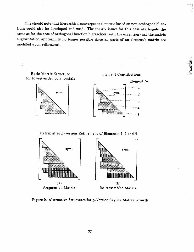
An interesting issue about economy of storage and factorization costs arises when
one considers the alternatives for growing the skyline matrix structure as the order of the
element functions grows. This issue is illustrated in Figure 9, where a basic skyline matrix
is shown along with two possible growth versions of the matrix. In the scenario depicted
on the left, the additional terms due to p-refinement have been simply added to the end
of the matrix. This alternative is referred to as the matrix augmentation approach. In
the scenario depicted on the right, the additional terms have been assembled directly into
the matrix interior. This alternative is called the matrix re-assembly approach. As can
be seen from the relative dimensions of the two matrices in the lower half of Figure 9, the
matrix on the right has a lower maximum bandwidth, a lower average bandwidth, and a
lower total profile. Presumably, factorization costs for the matrix on the right would be
less than for the matrix on the left, however, the factored portion of the matrix up to
the first row corresponding to added terms remains unaltered and can thus be re-used in
operations involving the factors of the augmented matrix.
Intuitively, it seems natural that some breakpoint would exist when the size of the ma-
trix and the number of additional terms due to p-refinement reach values that equalize the
cost of the two approaches; augmentation and partial factor]zation versus re:assembly and
complete factorization. Both methods would therefore be useful generally in p-version ele-
ments and algorithms. A skyline matrix structure could be made to admit both approaches
providing very general matrix assembly and matrix factoring utilities are developed. The
assembly would necessarily have to account for augmentation and insertion of matrix rows,
and the factoring would have to be able to begin from a partially factored matrix state. To
admit further research in the area of computational methods for p-version finite elements,
both schemes should be made available in any general package of matrix operations.
31
.... E!
One should note that hierarchicalconvergence elements based on non-orthogonal func-
tions could also be developed and used. The matrix issuesfor this case are largely the
same as for the case of orthogonal function hierarchies,with the exception that the matrix
augmentation approach is no longer possible since all parts of an element's matrix are
modified upon refinement.
Basic Matrix Structure
for lowest-order polynomials
m m
Element Contributions
u
li!!!iiii!iii!ii!iii!ii!iiiii
Element No.
- " ............. 1
...............
..................
............... 4
......... _ ..... 5
: £'._
_.
Matrix after p-version Refinement of Elements I, 2 and 5
m m
iiiiiiiii ijt,,,, (a)
Augmented Matrix
.::i:_f:':_:__..::_:_8k_:_:_:_:i::..
.'-::-_:-::i:_.::i::_:?-i:?-_-_:::_:i:::_:_-
IIllllIIIIIilIIIIIIIIIIIIIItlIIilIIIIN
(b)
Re-A ssembled Matrix
Figure 9. Alternative Structures for p-Version Skyline Matrix Growth
32
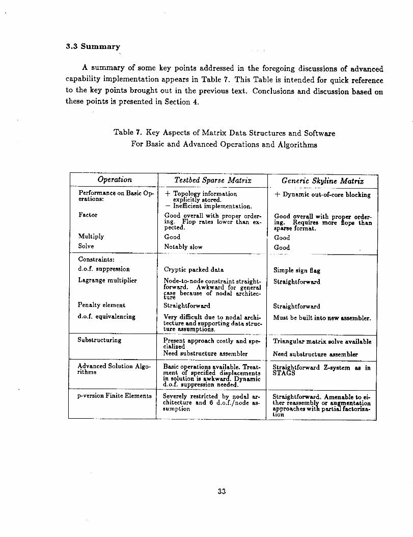
3.3 Summary
A summary of some key points addressed in the foregoing discussions of advanced
capability implementation appears in Table 7. This Table is intended for quick reference
to the key points brought out in the previous text. Conclusions and discussion based on
these points is presented in Section 4.
Table 7. Key Aspects of Matrix Data Structures and Software
For Basic and Advanced Operations and Algorithms
Operation Testbed Sparse Matrix Generic Skyline Matrix
-k Dynamic out-of-core blockingPerformance on Basic Op-erations:
Factor
Multiply
Solve
Constraints:
d.o.f, suppression
Lagrange multiplier
Penalty element
d.o.f, equivahncing
Substructuring
Advanced Solution Algo-rithms
p-versionFiniteElements
q- Topology informationexplieidy stored.
-- Inefficient implementation.
Good overall with proper order-ing. Flop rates lower than ex-pected.
Good
Notably slow
Cryptic packed data
Node-to-node constraint straight-forward. Awkward for generalfase because of nodal architec-l_ure
Straightforward
Very difficult due to nodal archi-tecture and supporting data struc-ture assumptions.
Present approach costly and spe-cializedNeed substructure assembler
Basicoperationsavailable.Treat-ment of specifieddisplacementsinsolutionisawkward. Dynamicd.o.f,suppressionneeded.
Severely restricted by nodal ar-chitecture and 6 d.o.f./node as-sumption
Good overall with proper order-ing. Requires more flops thansparse format.
Good
Good
Simple sign flag
Straightforward
Straightforward
Must be builtintonew assembler.
Triangular matrix solve available
Need substructure assembler
Straightforward Z-system as inSTAGS
Straightforward. Amenable to ei-ther reassembly or augmentationapproaches with partialfactoriza-tlon
33
4. Recommendations for Testbed Matrix Development
The preceding discussions focused on the extension of current Testbed capabilities to
accommodate a variety of advanced analysis capabilities. Assumed in this discussion was
that the characteristics of the most basic levels - the system matrix manipulation software
and data structures - determine the feasibility of upgrading of the Testbed's algorithmic
capabilities. This assumption is not strictly true, since high-level programming languages
afford sufficient flexibility to implement almost any scheme regardless of how intricate
or particular it may be. But given the stated purpose of the Testbed (to aid technology
advancement by integrating CSM research and development through a common, extendable
software architecture), the more basic approach seems more likely to succeed by laying a
solid foundation for further Testbed and CSM development. The discussion presented in
this section proceeds from this premise and focuses on defining a development path that
simultaneously assures flexibility in use and extension, and efficiency in operation.
This section is divided into three main parts. The first part discusses the implemen-
tation of new matrix data structures and associated computational facilities in the CSM
Testbed. Particular attention is given to the implementation of a generic skyline matrix.
The second part focuses on the design of a generic environment for further development
of matrix methods in the CSM Testbed and for incorporation of alternative useful matrix
data structures and computational modules. The third section contains some concluding
comments and observations about matrix methods development in the CSM Testbed.
4.1 Incorporation of New Matrix Schemes
Incorporating new matrix structures and computational utilities into the CSM Testbed,
whether to supplant or augment the present sparse matrix capability, requires several spe-
cific requirements to accommodate the advanced algorithms discussed in Section 2. These
requirements are:
1) A flexible, substructure-oriented topology analysis and system matrix
assembler. Critical features of the assembler include the ability to as-
semble diagonal and off-diagonal substructure matrix blocks, ability
to use degree of freedom or nodal resequencing lists calculated by
external utilities, and the ability to assemble only specified elements
and/or groups of elements. The ability to handle d.o.f.-equivalence
constraint matrices is desired, but not required, provided that a ca-
pability to assemble Lagrangian or penalty constraints is provided.
34
2) Matrix computational facilities to perform all of the basic operations
listed in Tables 2 and 5including a separate facility for either the
triangular matrix solve operation or direct computation of the Schur
complement. These facilities require a data interface to the Testbed
system-vector data structure.
3) A facility to enable the dynamic suppression of selected degrees of
freedom for use in conjunction with advanced nonlinear continuation
algorithms.
Any matrix data structure and associated computational software to be implemented
in the Testbed should be extensively documented as to structure and usage. Since the
CSM Testbed is to serve as an integrating platform for advanced methods, many of which
are yet to be defined in detail, the operational particulars of the Testbed software must be
as clear as possible. This requirement is especially critical with respect to matrix software
and data structures since mat_'ix algebra operations form the computational cornerstone
of numerical algorithms.
4.2 Incorporation of a Skyline Matrix Scheme
A logical first step toward providing advanced matrix capabilities in the CSM Testbed
would be the implementation of the generic skyline matrix data structure and utilities. This
development is supported primarily by considerations of flexibility and an unquantified no-
tion that algorithm development time and effort would be reduced through the availability
of a simple and flexible matrix data structure, particularly in cases where system matrix
data must be specially modified or accessed in algorithmic operations.
The adoption of a skyline matrix scheme will not adversely affect the computational
efficiency of matrix operations in the Testbed. The computational efficiency of well-coded
skyline matrix utilities is, at the very least, competitive with the Testbed sparse matrix
utilities, based on the results of the performance survey described in Section 3.1.2. The
primary advantages of the SKYNOM skyline matrix software from a performance stand-
point arises from its flexible use of memory resources to reduce I/O costs for out-of-core
solutions, and its native use of the GAL nominal data manager. Potential advantages also
should be noted for executions on vector processing computers, where the length of the
matrix row vectors in the skyline structure makes possible significant savings through the
use of vector arithmetic.
The flexibility of a skyline matrix data structure is due to its simplicity. The Testbed
sparse matrix structure is blocked into artificially fixed-length records, each an amalgam
of indexing and matrix data that cannot be decoded without access to external data
35
structures. The skyline matrix data structure, on the other hand, is self-contained and
separates indexing and matrix values data into two simple records. The entire structure of
the skyline matrix is available through examination of a single, system-vector-sized index.
The word-addressable capability of the GAL data manager makes access to portions of
the skyline matrix values record straightforward. A useful addition to the skyline matrix
data structure would be to incorporate topological data as discrete record groups in the
matrix dataset. These data would preferably describe the equation ordering of the matrix
and the element-equation connectivity. In cases of substructure matrices, lists of boundary
and interior nodes or degrees of freedom could also be stored......... L_ -- =
The major drawback of the skyline matrix structure is that it potentially requires
more external storage than a sparsely stored matrix. In cases where external storage is at
a premium relative to memory utilization and I/O activity, the sparse matrix makes more
sense. However, these cases appear only rarely and do not present a sufficient impediment
to preclude the adoption of a skyline matrix format for the stated reasons of efficiency and
flexibility.
The steps necessary to implement a skyline matrix system in the CSM Testbed closely
parallel those outlined in Section 4.1 and include:
1) Construction of a flexible skyline matrix assembly program. As noted
in the discussions of Section 3, an assembler processor capable of as-
sembling element matrices, full square matrices and skyline matrices
of different orders and topologies would be ideal. Also, a capability to
assemble vector blocks representing the off-diagonal coupling terms
(Kis) of substructured matrices should be included, along with the
capability to process d.o.f.-elimination type constraints. The develop-
mental steps necessary to implement these capabilities in the Testbed
are:
a)
b)
c)
Construction of modular subroutine or function entry
points to access Testbed element connectivity and matrix
data.
Construction of a basic skyline matrix assembler processor
to provide the same functionality as the present Testbed
sparse matrix assemblers K, KG and M plus the capability
to include previously assembled skyline matrices in a new
skyline matrix.
Addition of substructuring capability to the skyline ma-
trix assembler to assemble the off-diagonal matrix blocks.
36
d) Implementation of a means to define equivalenced con-
straint relations in some Testbed modeling processor and
to assemble skyline matrices subject to these constraints
in the skyline matrix assembler processor.
2) Construction of a utility-oriented skyline matrix processor to provide
all matrix functions of the Z-system (Section 3.2.5) and decoupled
forward-reduction and backward-substitution functions to assist in
the efficient implementation of substructuring procedures. This sys-
tem would ideally be based on the present SKYNOM software to
take best advantage of previous developments, particularly in the dy-
namic blocking of out-of-core matrix operations. The development
steps necessary to implement this facility are:
a) Extract SKYNOM kernel routines and place them in a
utility-oriented processor shell constructed for use with
the Testbed.
b) Implement dynamic equation suppression and enabling for
unfactored skyline matrices.
c) Implement a staged-factoring procedure to support l>-
version finite element development.
The functionality of the Testbed system would not be impaired during the execution of
the above development steps. To ensure this, work would progress on the basic capabilities
outlined in the above steps l(a), l(b) and 2(a) simultaneously. Once these steps were
completed, the skyline matrix system would encompass all of the present Testbed matrix
capabilities and could thus replace it entirely. Further developments would proceed in an
evolutionary manner with new capabilities (items l(c), l(d), 2(b) and 2(d), above) coming
on-line as available.
One should note that the prior existence of and experience with skyline matrix software
like SKYNOM and the STAGS Z-System are substantial benefits to the economy of the
implementation effort required for a Testbed skyline matrix capability.
4.3 Generic Environment for CSM Matrix Methods Development
Further extendability of matrix methods in the CSM Testbed would be greatly facili-
tated by a computational environment that would provide many useful functions to matrix
methods and algorithm developers. Such functions might include straightforward access
to element and system vector data, powerful utilities for local data management, and fa-
cilities for command-language interpretation. Collection of such functions under a single
processor umbrella would aid Testbed algorithm developers by unifying the context within
3?
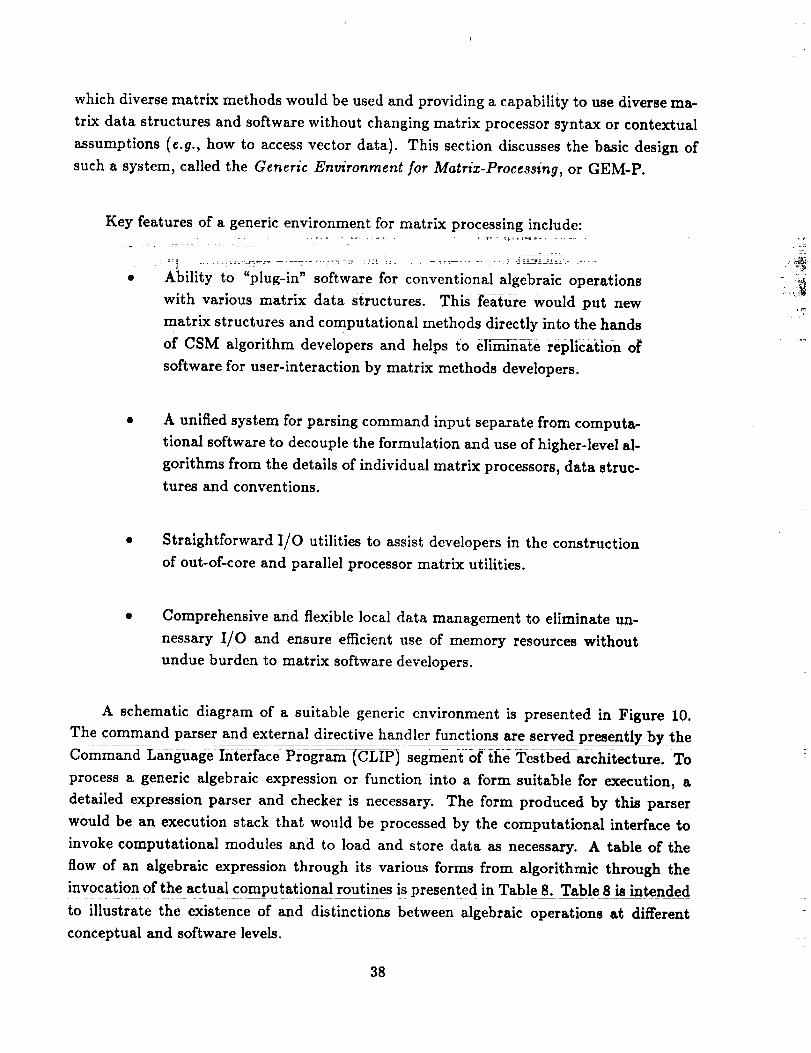
which diversematrix methodswould be usedand providing a capability to use diverse ma-
trix data structures and software without changing matrix processor syntax or contextual
assumptions (e.g., how to access vector data). This section discusses the basic design of
such a system, called the Generic Environment for Matrix-Processing, or GEM-P.
Key features of a generic environment for matrix processing include:
• Ability to _plug-in" software for conventional algebraic operations
with various matrix data structures. This feature would put new
matrix structures and computational methods directly into the hands
of CSM algorithm developers and helps to eliminate repiicat|on of
software for user-interaction by matrix methods developers.
A unified system for parsing command input separate from computa-
tional software to decouple the formulation and use of higher-level al-
gorithms from the details of individual matrix processors, data struc-
tures and conventions.
Straightforward I/O utilities to assist developers in the construction
of out-of-core and parallel processor matrix utilities.
Comprehensive and flexible local data management to eliminate un-
nessary I/O and ensure efficient use of memory resources without
undue burden to matrix software developers.
A schematic diagram of a suitable generic environment is presented in Figure 10.
The command parser and external directive handler functions are served presently_by the
Command Lahguage=L_terface Pro_am-_IP) segment of the--T_estbedarchitecture. To
process a generic algebraic expression or function into a form suitable for execution, a
detailed expression parser and checker is necessary. The form produced by this parser
would be an execution stack that would be processed by the computational interfaceto
invoke computational modules and to load and store data as necessary. A table of the
flow of an algebraic expression through its various forms from algorithmic through the
invocation of the actual computati_onal routines ispresented in Table 8. Table 8 isintended
to illustratethe existence of and distinctionsbetween algebraic operations at different
conceptual and software levels.
38
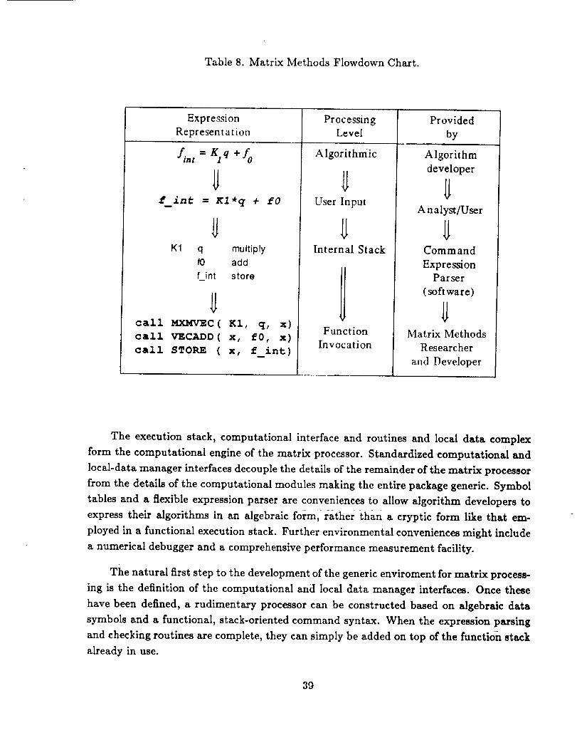
Table 8. Matrix Methods Flowdown Chart.
Expression
Representation
4nt=Sq+fo
Uf_int = Kl*q +
K1 q multiply
fO add
f_int store
fO
Ucall MXMVEC( K1, q, x)
call VECADD ( x, f0, x)
call STORE ( x, f_int)
ProcessingLevel
Algorithmic
UUser Input
UInternal Stack
Function
Invocation
Provided
by
Algorithm
developer
UA nalyst/User
UCommand
Expression
Parser
(soft ware)
UMatrix Methods
Researcher
and Developer
The execution stack, computational interface and routines and local data complex
form the computational engine of the matrix processor. Standardized computational and
local-data manager interfaces decouple the details of the remainder of the matrix processor
from the details of the computational modules making the entire package generic. Symbol
tables and a flexible expression parser are conveniences to allow algorithm developers to
express their algorithms in an algebraic form, rather than a cryptic form like that em-
ployed in a functional execution stack. Further environmental conveniences might include
a numerical debugger and a comprehensive performance measurement facility.
The natural first step to the development of the generic enviroment for matrix process-
ing is the definition of the computational and local data manager interfaces. Once these
have been defined, a rudimentary processor can be constructed based on algebraic data
symbols and a functional, stack-oriented command syntax. When the expression parsing
and checking routines are complete, they can simply be added on top of the function stack
already in use.
39
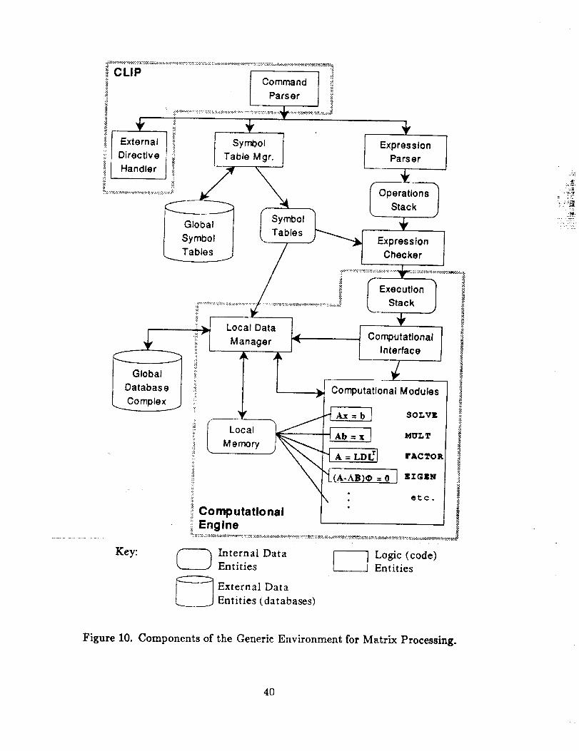
.;>:¢".¢.:-:-:.:-:.:-:_<.:.:.:+:-:.x.:.:+:.:.:.:+:.:.:.:.:.:+:.:..:.:.:...:....:. -:....:...x.:.:.:.:.:.- ,:._:_._:.:.:_.:.:.:.:+_.>:_=.:.:.:.;_:._.:::.:._.:...x._..+:._:_.:_.:: L
ii CLIP _iCommand _:_
Parser i!i
,xt°m.,l! l,,_bo, t " ,_0,..,ooj::i! Directive i!ii / Table Mgr. J Parser I
iii Handler j!!_ ..... _f i
12_ °' I , J_ E_0_.s,onr
/ i_.................._7::2::?................i:: L Stack J _
Looaoatar. I *!ii ' ,- Computational Modulesi_i - i: _ "_ Ax = b t SOLVg ;_!'_
_; Local
;_::(,. Memory I_ I Ab=x ] .UT-T
i! _ X_ t A = LDI_] I'ACTOg
\ etc.ii Computational
ii Engine
Key: _ Lnternal Data _ Logic (code)Entities Entities
_ External Data
Entities (databases)
,_oe
Figure 10. Components of the Generic Environment for Matrix Processing.
4O
4.4 Concluding Remarks
The purpose of the Testbed is to promote advanced methods research and development
for analyzing the aerospace structures of the 1990's using parallel and vector processing
computers. The present Testbed software must be enhanced to provide an environment for
advanced development. New flexible and extendable matrix data structures and utilities
are necessary to enable the Testbed to fulfill its role in the productive development of
improved computational structural mechanics algorithms.
A simple repackaging of the logic structures and functional organization of the SPAR
matrix processors in a modern, structured form is of limited value. The explicit nodal
orientation of the system matrix structure should be abandoned and all matrix operations
should be made available in the context of a single processor, rather than in the present
menagerie of TOPO, K, M, KG, INV, SSOL, AUS, SYN, etc. While the nodal orientation
of the system vectors is convenient from a usage standpoint, one should recognize that
it is the function of the finite-element formulations, not the matrix algebra software, to
translate the governing partial differential equations into an algebraic form. Requiring the
matrix software to conform to a specific finite-element context severely limits the algebraic
utility of the matrix software while providing only marginal convenience in conventional
executions. What is required is a different approach - one that ensures flexibility while
not sacrificing functionality or efficiency.
The advocated approach is to develop the generic environment for matrix processing,
discussed in Section 4.2. This approach is a departure from past, functionally oriented
approaches in that the matrix software environment is to be constructed without specific
reference to particular matrix data structures or software kernels. Instead, an accom-
modating standard interface set is to be used to allow multiple kernels to be referenced
within a single processor. Such an approach ensures a contextual uniformity to the invo-
cation of all matrix software and reduces the workload for any subsequent CSM researcher
implementing new matrix tools since user and database interfaces are provided with the
environment. One of the goals of this approach is to ensure that the _environmental"
software is not unduly burdened with overhead, so that the kernels themselves can be
optimized to produce run-time efficiency.
Finally, while this document does not address matrix data structures other than the
present Testbed sparse and a generic skyline structures, one should carefully consider other
organizations as well. For instance, frontal and multifrontal approaches are rapidly gaining
in popularity as reordering algorithms for these sparse structures are becoming more robust
and vectorization of multifrontal solvers has been accomplished with great success. These
matrix structures are certainly good candidates for implementation in the Testbed and
41

such an implementation would no doubt assist in the advancement of the state of the art
in computational structural mechanics. One should be cautious, however, at leaping to
the adoption of one particular structure in favor of all others since no one structure will
provide both the efficiency and the flexibility necessary to develop and exercise the wide
variety of CSM algorithms expected to result from research and development use of the
Testbed.
42
5. References
1. Stewart, Caroline B. (compiler): The Computational Structural Mechanics Testbed
User's Manual. NASA TM-100644, 1989.
2. Whetstone W. D.: Computer Analysis of Large Linear Frames. Journal of the Struc-
turalDimsion, ASCE, vol, 95, no. STll, November 1969, pp. 2401-2417.
3. Regelbrugge, Marc E. and Wright, Mary A.: The CSM Testbed Matrix Processors
Internal Logic and Dataflow Descriptions. NASA CR-181742, 1988.
4. Felippa, Carlos A.: Solution of Linear Equations with Skyline-Stored Symmetric Ma-
trix. Computers and Structures, vol. 5, 1978, pp. 13-29.
5. Wright, Mary A.; Regelbrugge, Marc E.; and Felippa, Carlos A.: The Computational
Structural Mechanics Testbed Architecture: Volume IV- The Global-Database Man-
ager GAL-DBM. NASA CR-178387, January 1989.
6. Gibbs, Norman E.; Poole, William G., Jr.; and Stockmeyer, Paul K.: An Algorithm for
Reducing the Bandwidth and Profile of a Sparse Matrix. SIAM Journal of Numerical
Analysis, vol. 13, no. 2, April 1976, pp. 236-250.
7. Stewart, Caroline B. (compiler): The Computational Structural Mechanics Testbed
Data Library Description. NASA TM-100645, 1988.
8. Felippa, Carlos A.: Iterative Procedures for Improving Penalty Function Solutions of
Algebraic Systems. International Journal for Numerical Methods in Engineering, vol.
12, 1978, pp. 821-836.
9. Whetstone, W. D.: SPAR Structural Analysis System Reference Manual, vols. i-4.
NASA CR 158970-1, December 1978.
10. Almroth, B. O.; Brogan, F. A.; and Stanley, G. M.: Structural Analysis of Gen-
eral Shells, vol. II - User Instructions for STAGSC-1, Report No. LMSC-D633873,
Lockheed Pals Alto Research Laboratory, Pals Alto, CA, December 1982.
11. Rankin, C. C.; Stehlin, P.; and Brogan, F. A.: Enhancements to the STAGS Computer
Code. NASA CR-4000, November 1986.
12. Riks, E.: On the Numerical Solution of Snapping Problems in the Theory of Elastic
Stability:SUDDAR Report No. 410, Stanford University,Stanford CA, 1970.
43
13. Riks, E.: Progress in Collapse Analysis, Journal of Pressure Vessel Teehnoloffy, ASME,
vol. 109, 1987, pp. 33-41.
14. Crisfield, M. A.: A Fast incremental/Iterative Solution Procedure that Handles Snap-
Through. Computers and Structures, vol. 13, 1983, pp. 55-62.
15. Thurston, G. A.; Brogan, F. A.; and Stehlin, P.: Postbuckling Analysis Using a
General-Purpose Code. AIAA Journal, vol. 24 no. 6, June 1986, pp. i013-1020.
16. Rankin, C. C. and Brogan, F. A.:: Application of the ThurSton Bifurcati0n Solution
Strategy to Problems with Modal Interaction. AIAA Paper No. 88-2286_ 1988,
44
Report Documentation Page
1.NASAReportCR-181951N°" 12. Government Accession No. 3. Reciptent's Catalog No.
4. Title and Subtitle
Comparison of Two Matrix Data Structures for Advanced CSM
Testbed Applications
7. Author(s)
M. E. Regelbrugge, F. A. Brogan, B. Nour-Omid, C. C. Rankin and
M. A. Wright
9. Performing Organization Name and Address
Lockheed Missiles and Space Company, Inc.
Research and Development Division3251 Hanover Street
Palo Alto, California 94304
12. Sponsoring Agency Name and Address
National Aeronautics and Space Administration
Langley Research Center
Hampton, VA 23665-5225
5. Report Date
December 1989
6. Performing Organization Code
8. Performing Organization Report No.
10. Work Unit No.
505-63-01-10
11. Contract or Grant No.
NAS1-18444
13. Type of Report and Period Covered
Contractor Report
14. Sponsoring Agency Code
15. Supplementary Notes
Langley Technical Monitors: W. Jefferson Stroud and Norman F. Knight, Jr.
16. Abstract
This document is divided into three sections. The first section describes data storage schemes presently
used by the CSM Testbed sparse matrix facilities and similar, skyline (profile) matrix facilities. The
second section contains a discussion of certain features required for the implementation of particular
advanced CSM algorithms, and how these features might be incorporated into the data storage schemes
described previously. The third section presents recommendations, based on the discussions of the prior
sections, for directing future CSM Testbed development to provide necessary matrix facilities for advanced
algorithm implementation and use.
17.Key Words (Suggestedby Authors(s))Structuralanalysis
Matrix methods
Substructuring
19. Security Classlf.(of this report)Unclassified
18. DistributionStatement
Unclassified--Unlimited
Subject Category 59
20. Security Classif.(of this page)Unclassified 21. No. of Pages ] 22. Price51 l A04NASA FORM 1616 oct se
For sale by the National Technical Informatlc, n Service, Springfield, Virginia 22161-2171