comparison of system identification techniques for the ... · nasa technical memorandum 110279...
TRANSCRIPT
NASA Technical Memorandum 110279
Comparison of System Identification Techniquesfor the Hydraulic Manipulator Test Bed (HMTB)
A. Terry Morris
Langley Research Center, Hampton, Virginia
September 1996
National Aeronautics and
Space AdministrationLangley Research CenterHampton, Virginia 23681-0001
https://ntrs.nasa.gov/search.jsp?R=19970001261 2020-04-02T23:33:52+00:00Z

Table of Contents
List of Tables ..................................................................................... iii
List of Figures ................................................................................... iv
Symbols and Acronyms ..................................................................... viii
go Introduction ............................................................................ 1
1. DOSS Background ........................................................ 2
2. Hydraulic Manipulator Test Bed (HMTB) ..................... 5
3. Remote Power Controller Module ................................. 8
4. System Identification Techniques .................................. 9
Ho Experiment Design ................................................................. 10
1. Overall Design Process ................................................. 10
2. Input Excitations ........................................................... 11
A. Description of Input Excitations ............................... 11
B. Generation of Input Excitations ................................ 18
3. Input Excitation and Control ......................................... 18
A. Single Joint Excitation ............................................. 19
B. Multiple Joint Excitation with Bias Compensation... 20
4. 1553 Bus Data Acquisition ........................................... 215. 1553 Bus Format to ASCII Conversion ......................... 22
Nonparametric Model Estimation .......................................... 23
1. Pr6cedure Description and Rationale ............................. 23
2. Shoulder Yaw Joint ....................................................... 24
A. Transfer Function Analysis ....................................... 24
B. Correlation Analysis ................................................. 26
C. Spectral Analysis ...................................................... 293. Shoulder Pitch and Elbow Pitch Joints ........................... 35
4. Nonparametric Conclusions ........................................... 35
IWi Parametric Model Estimation:
Transfer Function and State-Space System Identification ..... 361. Parametric Procedures .................................................... 36
2. Parametric Black-Box Models ........................................ 38
3. Identification of Shoulder Yaw Joint .............................. 39
A. Preliminary Model Estimates ..................................... 39
B. Determination of Best Model Estimate ....................... 46
C. SISO State-Space Estimate ........................................ 464. Identification of Shoulder and Elbow Pitch Joints ........... 47
5. State-Space Multivariable Representation ...................... 49
Vi Parametric Model Estimation:
Observer/Kalman Filter Identification ...................................
1. OKID Background and Procedure ..................................
2. Identification of Shoulder Yaw Joint ..............................
A. Determine Markov Parameter Set ..............................
B. OKID State-Space Estimate ......................................
C. Analysis ....................................................................
3. Identification of Shoulder and Elbow Pitch Joints ..........
4. State-Space Multivariable Representation ......................
Vii Comparison of Identified Models ............................................
2.
3.
4.
5.
6.
Identified Model Forms .................................................
Transfer Function Analysis ............................................
Pole/Zero Map ..............................................................
RPCM Fit Comparison ..................................................
M/MO Chirp Fit Comparison ........................................
Comparison Results ......................................................
VIIo Conclusions ..............................................................................
I. SuggestionsforFuture Work .........................................
2. Model Reference Control..............................................
References ..........................................................................................
Appendix A.A.1
A.2
A.3
Plots and Graphs .......................................................
Nonparametric Plots .....................................................
Classical Parametric Plots .............................................
OKID Parametric Plots .................................................
50
50
52
52
53
55
57
58
59
59
61
64
66
73.
79
82
82
82
84
85
86
101
112
ii

List of Tables
Table
Number
Table
Description
PageNumber
Table 1.
Table 2.Single-Input, Single-Output Tests.
Multi-Input, Multi-Output Tests.
2O
2O
111
List of Figures
Figure
NumberFigure
DescriptionPageNumber
Figure 1.
Figure 2.
Figure 3.
Figure 4.
Figure 5.
Figure 6.
Figure 7.
Figure 8.
Figure 9.
Figure 10.
Figure 11.
Figure 12.
Figure 13.
Figure 14.
Figure 15.
Figure 16.
Figure 17.
Figure 18.
Figure 19.
Figure 20.
Figure 21.
Figure 22.
Figure 23.
Figure 24.
Figure 25.
Figure 26.
Figure 27.
Figure 28.
Figure 29.
Figure 30.
Figure 31.
Figure 32.
Figure 33.
Figure 34.
Figure 35.
Figure 36.
Figure 37.
Figure 38.
Figure 39.
Space Station Freedom. 3
Canada's SSRMS and SPDM working on Freedom's truss. 3
NASA's Flight Telerobotic Servicer fiTS). 4
LaRC's Hydraulic Manipulator Test Bed (HMTB). 5
The Hydraulic Manipulator Test Bed Setup. 6
The HMTB Hydraulic Manipulator. 6
The Aft Flight Deck (AFD). 7
Internal view of AFD mockup. 7
Remote Power Controller Module (RPCM) ORU. 8
Overall Experiment Design. 10
Simulated White Noise. 12
Sum of Sinusoids. 14
PSD of Sum of Sinusoids. 14
(a) Pseudorandom Binary Sequence (b) PSD of PRBS. 15
(a) Chirp Waveform (b) PSD of Chirp Waveform. 17
(a) Bipolar Ramping Pulse (b) PSD of BRP. 17
Waveform Generation Software User Interface. 18
Single Axis Interface Configuration. 19
Multiple Axes Interface with Bias Compensation. 21
Shoulder Yaw Sum of Sinusoids UO at 10 Hertz. 24
Shoulder Yaw Sum of Sinusoids Activity. 25
Shoulder Yaw Transfer Function Estimate. 26
Shoulder Yaw PRBS Data. 27
Shoulder Yaw PRBS Activity. 28
Shoulder Yaw Correlation Plots. 28
Shoulder Yaw Bipolar Ramping Pulse Data. 29
Shoulder Yaw Estimated Disturbance Spectrum. 30
Shoulder Yaw Estimated Output Spectrum. 30
Shoulder Yaw Estimated Input Power Spectrum. 31
Shoulder Yaw Estimated Cross-Spectrum. 31
Shoulder Yaw Sum of Sinusoids Input. 32
Shoulder Yaw Sum of Sinusoids Activity. 32
Shoulder Yaw Estimated Disturbance Spectrum. 33
Shoulder Yaw Estimated Output Spectrum. 33
Shoulder Yaw Estimated Input Power Spectrum. 34
Shoulder Yaw Estimated Cross-Spectrum 34
System Identification Process. 36
System Identification Operator Interface. 37
Shoulder Yaw ARMAX Residuals. 40
iv
Figure40.
Figure 41.
Figure 42.
Figure 43.
Figure 44.
Figure 45.
Figure 46.
Figure 47.
Figure 48.
Figure 49.
Figure 50.
Figure 51.
Figure 52.
Figure 53.
Figure 54.
Figure 55.
Figure 56.
Figure 57.
Figure 58.
Figure 59.
Figure 60.
Figure 61.
Figure 62.
Figure 63.
Figure 64.
Figure 65.
Figure 66.
Figure 67.
Figure 68.
Figure 69.
Figure 70.
Figure 71.
Figure 72.
Figure 73.
Figure 74.
Figure 75.
Figure 76.
Figure 77.
Figure 78.
Figure 79.
Figure 80.
Figure 81.
Shoulder Yaw
Independence.
Shoulder Yaw
Shoulder Yaw
Shoulder Yaw
Shoulder Yaw
Shoulder Yaw
Shoulder Yaw
Shoulder Yaw
ARMAX Residual Whiteness and
ARMAX Pole-Zero Plot.
ARMAX Output Comparison.
ARMAX Cross-Validation.
OE Residuals.
OE Residual Whiteness and Independence.OE Pole-Zero Plot.
OE Output Comparison.Shoulder Yaw OE Cross-Validation.
Bode Plots of the _, ARX, and OE Estimates.
Shoulder Yaw System and Observer Markov Parameters.
Shoulder Yaw Output Prediction Errors.
Shoulder Yaw Hankel Matrix.
Shoulder Yaw Bode Plot of State-Space Estimate.
Shoulder Yaw Predicted Versus Measured Output.
Shoulder Yaw Chirp Cross-Validation.
ARMAX Structure Block Diagram.
OE Structure Block Diagram.
SyslD Shoulder Yaw Bode Plots.
SyslD Shoulder Pitch Bode Plots.
SysID Elbow Pitch Bode Plots.OKID Shoulder Yaw Bode Plots.
OKID Shoulder Pitch Bode Plots.
OKID Elbow Pitch Bode Plots.
SysID Multivariable Model Pole/Zero Map.
OKID Multivariable Model Pole/Zero Map.
Multivariable RPCM Experiment Data.
SyslD RPCM Shoulder Yaw Comparison.
SyslD RPCM Shoulder Pitch Comparison.
SyslD RPCM Elbow Pitch Comparison.
SyslD RPCM MIMO Residuals.
SysID Shoulder Yaw and Pitch Residual Whiteness.
SysID Elbow Pitch Whiteness and Shoulder Yaw
Independence.
OKID RPCM Shoulder Yaw Comparison.
OKID RPCM Shoulder Pitch Comparison.
OKID RPCM Elbow Pitch Comparison.
OKID RPCM M/MO Residuals.
OKID Shoulder Yaw and Pitch Residual Whiteness.
OKID Elbow Pitch Whiteness and Shoulder Yaw
Independence.
Multivariable Chirp Experiment Data.
SysID Chirp Shoulder Yaw Comparison.
SysID Chirp Shoulder Pitch Comparison.
40
41
42
42
43
44
44
45
45
46
53
54
54
55
56
56
60
60
61
62
62
63
63
64
65
65
66
67
67
68
68
69
69
70
71
71
72
72
73
74
75
75
Figure82.Figure83.Figure84.
Figure 85.
Figure 86.
Figure 87.
Figure 88.
Figure A1.
Figure A2.
Figure A3.
Figure A4.
Figure A5.
Figure A6.
Figure A7.
Figure A8.
Figure A9.
Figure A10.
Figure A11.
Figure A12.
Figure A13.
Figure A14.
Figure A15.
Figure A16.
Figure A17.
Figure A18.
Figure A19.
Figure A20.
Figure A21.
Figure A22.
Figure A23.
Figure A24.
Figure A25.
Figure A26.
Figure A27.
Figure A28.
Figure A29.
Figure A30.
Figure A31.
Figure A32.
Figure A33.
Figure A34.
Figure A35.
Figure A36.
SysID Chirp Elbow Pitch Comparison.
SysID MIMO Chirp Residuals.
OKID Chirp Shoulder Yaw Comparison.
OKID Chirp Shoulder Pitch Comparison.
OKID Chirp Elbow Pitch Comparison.
OKID M/MO Chirp Residuals.
Model Reference Control System for DOSS.Shoulder Pitch I/O Data.
Shoulder Pitch Transfer Function Estimate.
Shoulder Pitch PRBS Data.
Shoulder Pitch Correlation Plots.
Shoulder Pitch Bipolar Ramping Pulse Data.
Shoulder Pitch BRP Activity.
Shoulder Pitch Estimated Disturbance Spectrum.
Shoulder Pitch Estimated Output Spectrum.
Shoulder Pitch Estimated Input Power Spectrum.
Shoulder Pitch Estimated Cross-Spectrum.
Shoulder Pitch Sum of Sinusoids Activity.
Shoulder Pitch Estimated Disturbance Spectrum.
Shoulder Pitch Estimated Output Spectrum.
Shoulder Pitch Estimated Input Power Spectrum.
Shoulder Pitch Estimated Cross-SpectrumElbow Pitch I/O Data.
Transfer Function Estimate.
PRBS Data.
Correlation Plots.
Bipolar Ramping Pulse Data.
Estimated Disturbance Spectrum.
Estimated Output Spectrum.
Estimated Input Power Spectrum.
Estimated Cross-Spectrum
Sum of Sinusoids I/0 Data.
Estimated Disturbance Spectrum.
Estimated Output Spectrum.
Estimated Input Power Spectrum.
Estimated Cross-SpectrumARMAX Residuals.
ARMAX Residual Whiteness and
Elbow Pitch
Elbow Pitch
Elbow Pitch
Elbow Pitch
Elbow Pitch
Elbow Pitch
Elbow Pitch
Elbow Pitch
Elbow Pitch
Elbow Pitch
Elbow Pitch
Elbow Pitch
Elbow Pitch
Shoulder Pitch
Shoulder Pitch
Independence.Shoulder Pitch
Shoulder Pitch
Shoulder Pitch
ARMAX Pole-Zero Plot.
ARMAX Output Comparison.
ARMAX Cross-Validation.
Shoulder Pitch OE Residuals.
Shoulder Pitch OE Residual Whiteness and
Independence.
76
76
77
78
78
79
83
86
86
87
87
88
88
89
89
90
90
91
91
92
92
93
93
94
94
95
95
96
96
97
97
98
98
99
99
100
101
101
102
102
103
103
104
vi
FigureA37.FigureA38.FigureA39.FigureA40.FigureA41.FigureA42.
FigureA43.FigureA44.FigureA45.FigureA46.FigureA47.FigureA48.FigureA49.FigureA50.FigureA51.FigureA52.FigureA53.FigureA54.FigureA55.FigureA56.FigureA57.FigureA58.FigureA59.FigureA60.FigureA61.FigureA62.FigureA63.
ShoulderPitchOE Pole-Zero Plot. 104
Shoulder Pitch OE Output Comparison. 105Shoulder Pitch OE Cross-Validation. 105
Bode Plots of the ARMAX, ARX, and OE Estimates. 106
Elbow Pitch ARMAX Residuals. 106
Elbow Pitch ARMAX Residual Whiteness and
Independence. 107Elbow Pitch ARMAX Pole-Zero Plot. 107
Elbow Pitch ARMAX Output Comparison. 108Elbow Pitch ARMAX Cross-Validation. 108
Elbow Pitch OE Residuals. 109
Elbow Pitch OE Residual Whiteness and Independence. 109Elbow Pitch OE Pole-Zero Plot. 110
Elbow Pitch OE Output Comparison. 110Elbow Pitch OE Cross-Validation. 111
Bode Plots of the ARMAX, ARX, and OE Estimates. 111
Shoulder Pitch System and Observer Markov Parameters. 112
Shoulder Pitch Output Prediction Errors. 112
Shoulder Pitch Hankel Matrix. 113
Shoulder Pitch Bode Plots of State-Space Estimate. 113
Shoulder Pitch Predicted Versus Measured Output. 114
Shoulder Pitch Chirp Cross-Validation. 114
Elbow Pitch System and Observer Markov Parameters. 115
Elbow Pitch Output Prediction Errors. 115
Elbow Pitch Hankel Matrix. 116
Elbow Pitch Bode Plots of State-Space Estimate. 116
Elbow Pitch Predicted Versus Measured Output. 117
Elbow Pitch Chirp Cross-Validation. 117
vii

Symbols
C,_(r )
caoe(t)
EI]fG(q),n(z)
Ha,)
H(o.)K
]d
0
¢Ru(n)
R_(v)
¢(w)u(t)vaov(t)v(o )W
w(OxaO
y(t)A
y(t)Y
Y
AcronymsAFD
ARMAX
ARX
BRP
BW
CSA
DOF
DOSS
ERA
ESA
Symbols and Acronyms
covariance function
damping ratio
residuals (equation errors)white noise
expectation operator
frequency
transfer function
Hankel matrix
disturbance dynamics
Kalman filter gain
mean
parameter vector
phase
autocorrelation matrix
cross-correlation function
spectral density function
input signal
input vector
disturbances
loss function
radian frequency
simulated white noise processstate vector
estimate of state vector
estimated measurement
measured output
predicted output
system Markov parameters
observer Markov parameters
Aft Flight Deck
Autoregressive Moving Average with Exogenous Variables
Autoregressive with Exogenous Variables
Bipolar Ramping PulseBandwidth
Canadian Space Agency
Degree of Freedom
Dexterous Orbital Servicing System
Eigensystem Realization Algorithm
European Space Agency
..°
viii

ESD
EVA
FFT
FTS
GND
HC
HMTB
IBM
IV4
JEM
LaRC
LSE
MEM
MIMO
MIO
MMAG
MPESS
MSS
NASA
OE
OKID
ORU
PC
PE
PEM
PRBS
PSD
RPCM
SISO
SOCIT
SPDM
SSF
SSRMS
STS
SyslDWSM
Emergency Shutdown
Extravehicular Activity
Fast Fourier Transform
Flight Telerobotic ServicerGround
Hand Controller
Hydraulic Manipulator Test BedInternational Business Machines
Four Stage Instrument Variable
Japanese Experiment Module
Langley Research Center
Least Squares Estimate
Maximum Entropy Method
•Multi-Input, Multi-Output
Multi Input/Output
Martin Marietta Astronautics Group
Multi-purpose Experiment Support Structure
Mobile Servicing System
National Aeronautics and Space Administration
Output ErrorObserver/Kalman Filter Identification
Orbital Replacement Unit
Personal Computer
Persistently ExcitingPrediction Error Method
Pseudorandom Binary Sequence
Power Spectral DensityRemote Power Controller Module
Single-Input, Single-Output
System/Observer/Controller Identification Toolbox
Special Purpose Dexterous Manipulator
Space Station Freedom
Space Station Remote Manipulator System
Space Transportation System
System Identification
Western Space and Marine
ix

L Introduction
The main objective of this thesis is to identify dynamical models of the Hydraulic
Manipulator Test Bed (HMTB). In particular, system identification techniques will be
used to identify the joint dynamics and to validate the correctness of the HMTB models.
Though dynamic model verification has been studied and performed for the DOSS flight
manipulator, dynamic system identification for the hydraulic kinematically-equivalent
ground-based DOSS manipulator located in the hydraulic manipulator test bed (HMTB)
facility at the NASA Langley Research Center has not been studied in detail. This thesis
will describe, apply, and compare system identification techniques for three joints
(shoulder yaw, shoulder pitch, and elbow pitch) of the seven DOF hydraulic manipulator
for the purpose of obtaining an adequate dynamic model of HMTB during insertion of the
remote power controller module ORU.
To perform the identification, a series of single-input, single-output (SISO) and
multi-input, multi-output (MIMO) experiments will be performed. Nonparametric and
parametric identification techniques will be explored in order to develop representative
models of the selected joints. The identified SISO model estimates will be validated. The
best performing models will be used for a decoupled multivariable state-space model. It
should be noted that each identified model represents an open-loop representation of the
closed-loop implementation for each joint. It is not the purpose of this thesis to determine
the effective inertia or the effective damping coefficients for the HMTB links. The
manipulator is localized about a representative space station orbital replacement unit
(ORU) exchange task allowing the use of linear system identification methods. The
parametric models will be compared to determine the best dynamic model for performingthe ORU task.
System identification techniques have been applied in many different fields. The
purpose of the identified models in this thesis is to use them in a control application. The
thesis concludes by proposing a model reference control system to aid in astronaut ground
tests. This approach would allow the identified models to mimic on-orbit dynamic
characteristics of the actual flight manipulator thus providing astronauts with realistic on-
orbit responses to perform space station tasks in a ground-based environment.
The process of system identification starts by performing an identification
experiment, that is, exciting the system using some sort of input signal and observing the
output over a time interval [9]. Once the experimental data is recorded, parametric or
nonparametric analysis can be performed. In nonparametric analysis, a system's transfer
function, impulse response, or step response is extracted from the experimental data in
order to determine transient or frequency response characteristics of the system. This
method, however, is often sensitive to noise and usually does not give very accurate
results [9]. In parametric analysis, the recorded input and output sequences are fitted to a
parametric model. This process begins by determining an appropriate model form. Next,
some statistically based method is used to estimate the unknown parameters of the model.
The model is then tested or validated to determine if it appropriately represents the
dynamic system.
The remainder of this chapter provides historical background of the DOSS
manipulator, the Hydraulic Manipulator Test Bed (HMTB) housed at the NASA Langley

ResearchCenter, and the orbital replacement unit hardware used by the manipulator.
Most of this information has not been published before. The chapter concludes by
providing a literature search on system identification techniques used in this thesis.
Chapter II will describe the overall experiment design process developed
specifically for the hydraulic manipulator test bed (HMTB). As a precursor to parametric
identification, Chapter III will describe the application of nonparametric methods used to
extract characteristics of the unknown joints. Parametric model estimation techniques
primarily used for control system identification will be applied in Chapter IV. In this
technique, transfer function models describing each joint and its associated disturbances
are analyzed to yield an adequate state-space model approximation. The second
parametric technique, used primarily in modal system identification, will be employed in
Chapter V. This technique uses a minimum realization algorithm to determine a model
with the smallest state-space dimension among all realizable systems. Comparisons of the
parametric models will be shown in Chapter VI. Chapter VII concludes the thesis by
providing suggestions for future work. A model reference control system is proposed to
provide astronauts with realistic on-orbit responses to perform space station tasks on theground.
Matlab menu-driven system identification software programs were developed for
this project. One of the programs, a menu-driven script written for nonparametric and
parametric evaluation of the input/output data using functions from the MA TLAB System
Identification Toolbox. Another menu-driven program was used to identify models using
the Observer/Kalman Filter Identification (OKID) technique, provided in the
System�Observer�Controller Identification Toolbox (SOCIT). This last program script
used several toolboxes to perform MIMO comparisons for identified models.
1. Dexterous Orbital Servicing System (DOSS) Background
In 1984 President Reagan directed the National Aeronautics and SpaceAdministration (NASA) to build a space station. He invited allies of the United States to
join in the challenge of creating a machine that could be manned and operated beyond the
year 2000 [1]. Space Station Freedom shown in Figure 1 was the first major co-operative
program of the governments of the U.S., Japan, the 10 nations of the European Space
Agency (ESA), and Canada for the utilization and operation of a microgravity laboratory
environment in space. Each government was responsible for furnishing specific user
elements of Space Station Freedom. The United States through the direction of the
National Aeronautics and Space Administration (NASA) was responsible for the design,
development, and construction of the truss assembly infrastructure, the crew living
quarters (US Habitat Module), and the US Laboratory Module. Japan would develop and
assemble the Japanese Experiment Module (JEM). The European Space Agency (ESA)
and its member states would develop their own Free-Flying Laboratory named Columbus
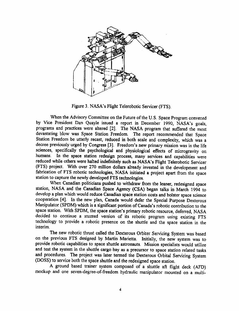
and a polar platform. Canada's responsibility involved providing the Mobile Servicing
System (MSS), a complex robotic machine used to assemble, service, and maintain most
of the station. The MSS's major robotic components are the Space Station Remote
Manipulator System (SSRMS) and the Special Purpose Dexterous Manipulator (SPDM)shown in Figure 2.
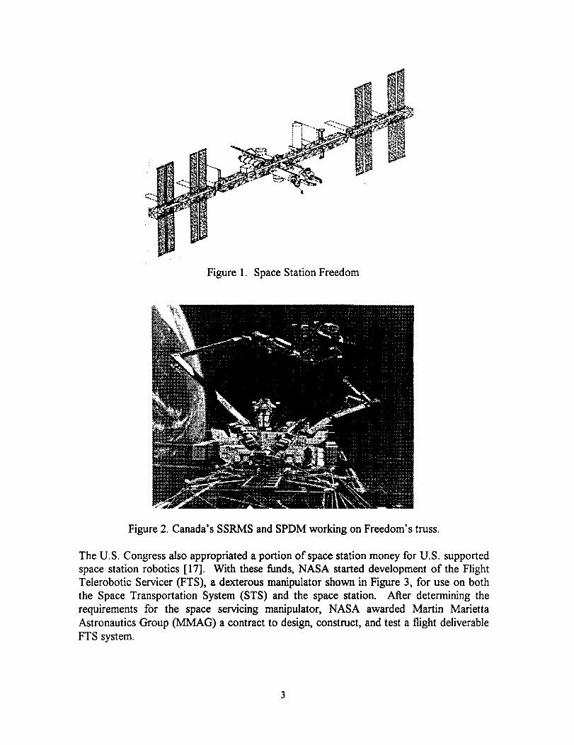
Figure1. SpaceStationFreedom
Figure 2. Canada's SSRMS and SPDM working on Freedom's truss.
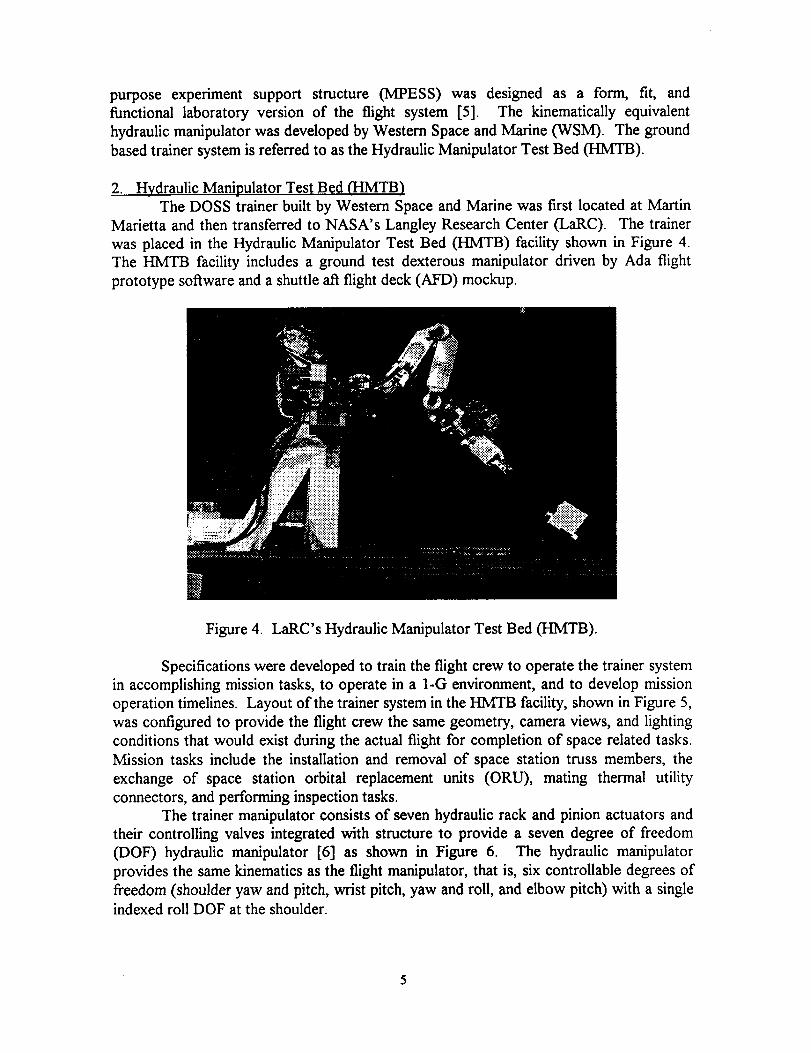
The U.S. Congress also appropriated a portion of space station money for U.S. supported
space station robotics [ 17]. With these funds, NASA started development of the Flight
Telerobotic Servicer (FTS), a dexterous manipulator shown in Figure 3, for use on both
the Space Transportation System (STS) and the space station. After determining the
requirements for the space servicing manipulator, NASA awarded Martin Marietta
Astronautics Group (MMAG) a contract to design, construct, and test a flight deliverable
FTS system.
A/
f
Figure 3. NASA's Flight Telerobotic Servicer (FTS).
When the Advisory Committee on the Future &the U.S. Space Program convened
by Vice President Dan Quayle issued a report in December 1990, NASA's goals,
programs and practices were altered [2]. The NASA program that suffered the most
devastating blow was Space Station Freedom. The report recommended that Space
Station Freedom be utterly recast, reduced in both scale and complexity, which was a
decree previously urged by Congress [3]. Freedom's new primary mission was in the life
sciences, specifically the psychological and physiological effects of microgravity on
humans. In the space station redesign process, many services and capabilities were
reduced while others were halted indefinitely such as NASA's Flight Telerobotic Servicer
(FTS) project. With over 270 million dollars already invested in the development and
fabrication of FTS robotic technologies, NASA initiated a project apart from the spacestation to capture the newly developed FTS technologies.
When Canadian politicians pushed to withdraw from the leaner, redesigned space
station, NASA and the Canadian Space Agency (CSA) began talks in March 1994 to
develop a plan which would reduce Canadian space station costs and bolster space science
cooperation [4]. In the new plan, Canada would defer the Special Purpose Dexterous
Manipulator (SPDM) which is a significant portion &Canada's robotic contribution to the
space station. With SPDM, the space station's primary robotic resource, deferred, NASA
decided to continue a stunted version of its robotic program using existing FTS
technology to provide a robotic presence on the shuttle and the space station in theinterim.
The new robotic thrust called the Dexterous Orbiter Servicing System was based
on the previous FTS designed by Martin Marietta. Initially, the new system was to
provide robotic capabilities to space shuttle astronauts. Mission specialists would utilize
and test the system in the shuttle cargo bay as a precursor to space station related tasks
and procedures. The project was later termed the Dexterous Orbital Servicing System
(DOSS) to service both the space shuttle and the redesigned space station.
A ground based trainer system composed of a shuttle ai_ flight deck (AFD)
mockup and one seven-degree-of-freedom hydraulic manipulator mounted on a multi-
4
purpose experimentsupport structure (MPESS) was designed as a form, fit, and
functional laboratory version of the flight system [5]. The kinematically equivalent
hydraulic manipulator was developed by Western Space and Marine (WSM). The ground
based trainer system is referred to as the Hydraulic Manipulator Test Bed (HMTB).
2. Hydraulic Manipulator Test Bed (HMTB)
The DOSS trainer built by Western Space and Marine was first located at Martin
Marietta and then transferred to NASA's Langley Research Center (LaRC). The trainer
was placed in the Hydraulic Manipulator Test Bed (HMTB) facility shown in Figure 4.
The HMTB facility includes a ground test dexterous manipulator driven by Ada flight
prototype software and a shuttle aft flight deck (AFD) mockup.
.ii:
Figure 4. LaRC's Hydraulic Manipulator Test Bed (HMTB).
Specifications were developed to train the flight crew to operate the trainer system
in accomplishing mission tasks, to operate in a 1-G environment, and to develop mission
operation timelines. Layout of the trainer system in the HMTB facility, shown in Figure 5,
was configured to provide the flight crew the same geometry, camera views, and lighting
conditions that would exist during the actual flight for completion of space related tasks.
Mission tasks include the installation and removal of space station truss members, the
exchange of space station orbital replacement units (ORU), mating thermal utility
connectors, and performing inspection tasks.
The trainer manipulator consists of seven hydraulic rack and pinion actuators and
their controlling valves integrated with structure to provide a seven degree of freedom
(DOF) hydraulic manipulator [6] as shown in Figure 6. The hydraulic manipulator
provides the same kinematics as the flight manipulator, that is, six controllable degrees of
freedom (shoulder yaw and pitch, wrist pitch, yaw and roll, and elbow pitch) with a single
indexed roll DOF at the shoulder.
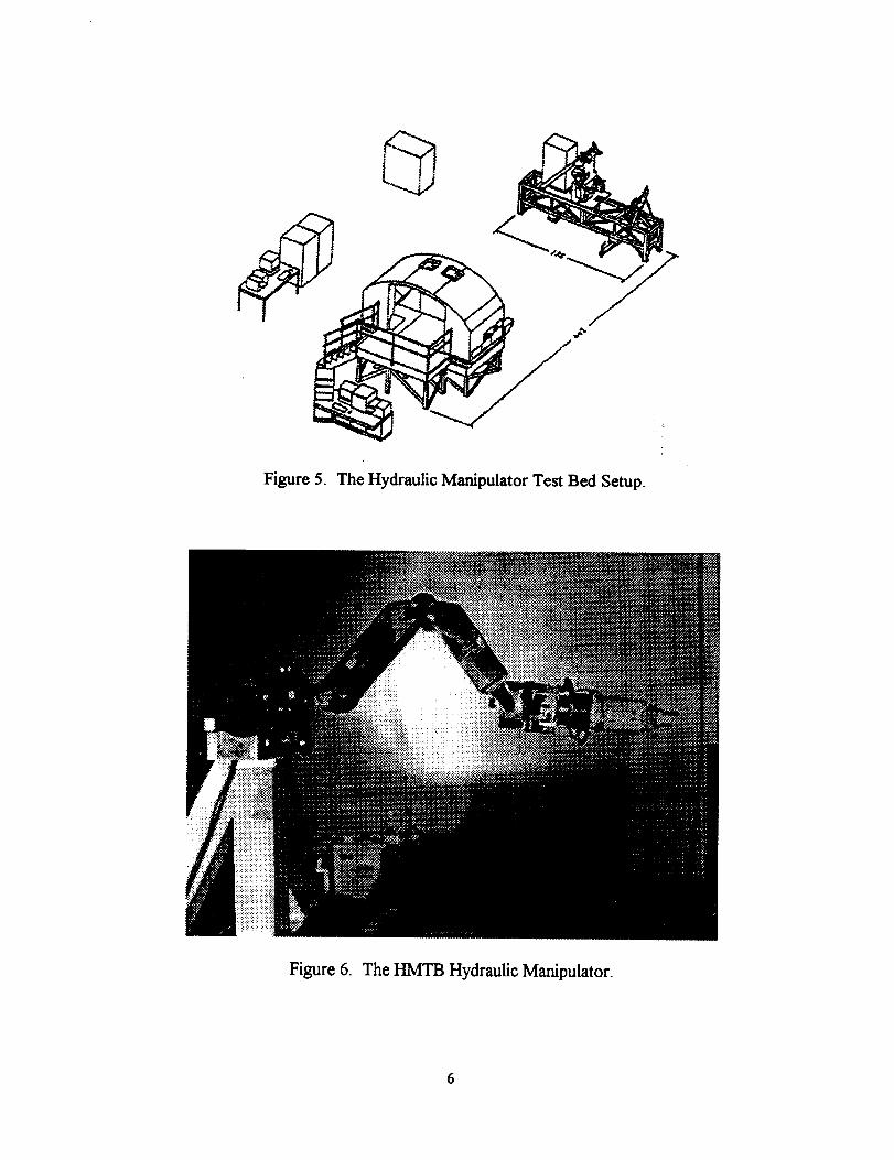
Figure5. The Hydraulic Manipulator Test Bed Setup.
Figure 6. The HMTB Hydraulic Manipulator.
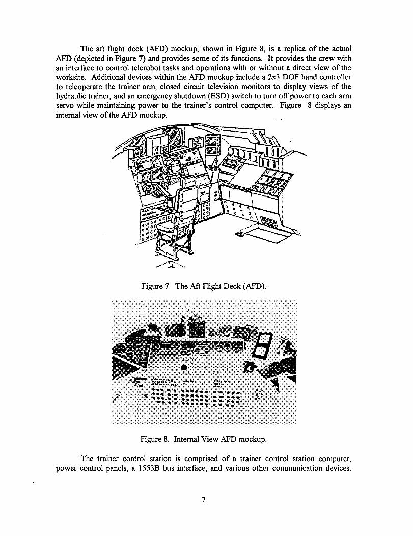
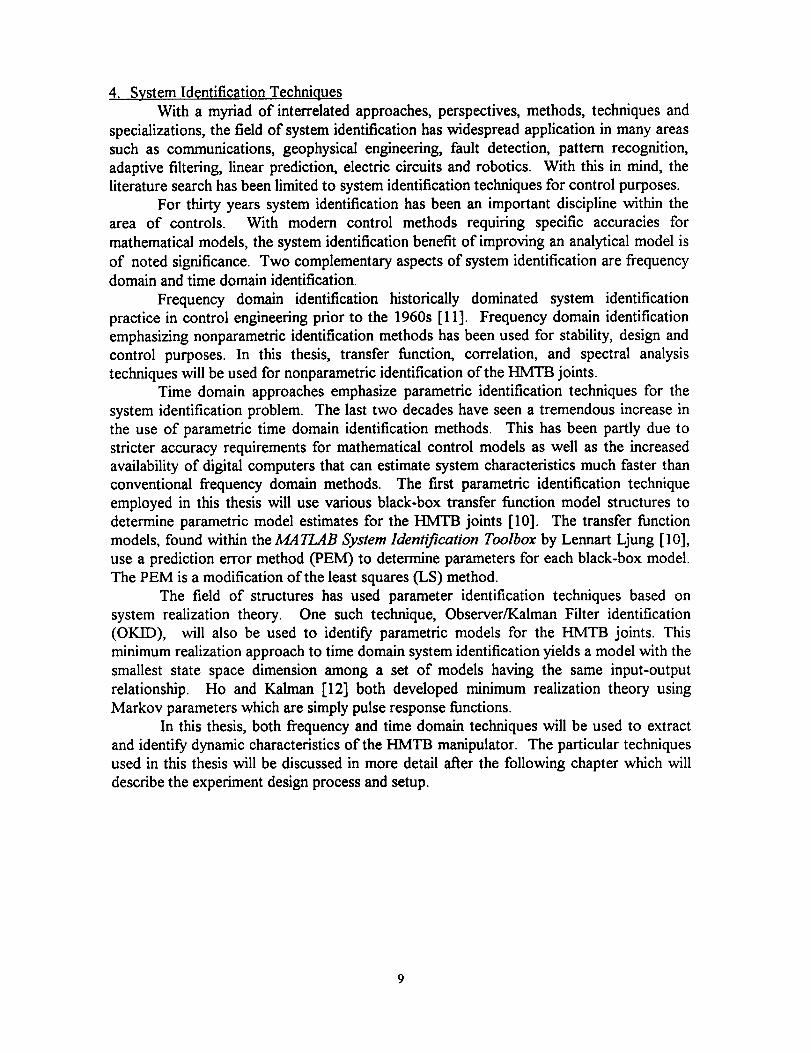
The ai_ flight deck (AFD) mockup, shown in Figure 8, is a replica of the actual
AFD (depicted in Figure 7) and provides some of its functions. It provides the crew with
an interface to control telerobot tasks and operations with or without a direct view of the
worksite. Additional devices within the AFD mockup include a 2x3 DOF hand controller
to teleoperate the trainer arm, closed circuit television monitors to display views of the
hydraulic trainer, and an emergency shutdown (ESD) switch to turn offpower to each arm
servo while maintaining power to the trainer's control computer. Figure 8 displays an
internal view of the AFD mockup.
Figure 7. The Aft Flight Deck (AFD).
i8: !:: :.:: :_:_!! i?i?!:: i : :.:_ :::!:::!:i:_:i:i:!:i:i:!:i:i:!:i:i:i:i:::_81:i:_:i:!:_:i-i:_:i:::::i:i:_:i:i:i:i:i:!i:i:i:i:i:i:_:18_:i:i:_:i:i:_:i:i:i:i:i:i:_:i:i:_:i:i?1:181:1:!:71:i:_:i:i:_:i:i:i:i:i:!:?i:i:_:!-i:!:i:i:i:?i:i:i:!:i:i:!:i:!:?i_i:i:i
i_!iiiii!i!i!i!i_i!iii!i!iii!ii!ii_ii!iiiiiiiiii!_i_iiiiii_i!i!i__ii_i_!_i__ii_!_ii!___!i!iii!i_i!i!i_i__!_iiii_iii_!!i_i!ii_i___i_!_!_i_!ii!__!ii_ii_ii_!i!_i_i_!ii_!_!_!_!_i_ii!_!i!i!___iiii!iiii_!ii_iii___i_i_i___!_i_i_i_iii_!ii_!_i!i_iii!!!!____i!i_____!__i!__iii_iii_!iiiiii!!!!
i i i i ii ii iii iii iiii iii iiiiiiii ii i ii! iiiiiiii iii ii i Eii / i iiiiiiiiiiiiiiiiiiiiiiiiiii iiiiiiiiiiiiiii iii iiiiiiiiiiiiiiiiiiiiiiiiiiiiiii iiiiiiiiiiiiiii!iiiiiiiiii i iiiiii ii ii i i i ii ::::i_!i!i_....... _ !i.iilg_.i.:.i::.:_:::>_:?!.................
!:_i!i !_i_i!_"" :i:..... "il _: 7k" _i: .. "" :::::::::::::::::::::::::::::::::::::::::::::::::
::::::::::::::::::::::::::::::::::::::::::::::::::::::: ::::: ::::: . ::::::-::: ::. 6 .:_111.:_1_:: ::_!_::::11_::;:;11_d_ _: : ;::: : : : : : : :. :.:._._:;::: :. : :.. :.. : : : :. : :: :::_,..:'?:.::: :.::.:: : ::::::::::::::::::::::::::::.:.: ...._:_..:'!_.._::..:_ _:'.1_'_ _: ':' *_:' _i _'"'" ":'_ ":_ _' _':":.................. :' :'::-':!:!_::i:_i: :: : !: !:i:!:!iiii:i:i!:_i!i!i_ii:iii:i_i_i_K_:i_ _? ::: :F :_!:_8. :8 _ :i:_:_ .-.: Q i:_:_:i:i:i:i:!:_:i:i:_:!:i:i8!:i:!:!:!:!:!:i:_Si:i:!:i:!:i:i:i:!8 !:_:i::!:!:!:: :: :: i:i: ::i:i::i:i::::::::_:i:i:::::i:i:::i:::::::::i:::_::::::::::::::::::::::::::::::::8::::_:_ i._: _: ._.::_:i._:_ :i_:i: [:_ ,ll _:[:i:!:_:i:iS_:_:!:i:i8 !:i:_:_:i:_:_:_:_:_:_:_:_:_:_:i:_:_:_8i:i:_:_:i:i:_i_:_:_:i:i:_:
:i:: :i:i: :i:i::i:i:: :i: :i:i:!:i:!:!:i:i:i::!:!:!:!:i:!:!:!:!:!8 !:!:!:i:i:!:!:i:!:!:!:!:i:!:!:i:!:!:i:i:!8!:!8 i:_:!:i:i:!8 !:i8 i:i:!:i:i:i:i:!:i:i:i8i:i:!:i:i:i8 _:_:_:i:_8 i:i:i:i:i:i:_:_:!:_:i:_;_:_:i:_81:i8i:i8 i:i:i8 i:i8i:i :_:i:!:i:?:i:_:_:: 81:i
_i::i::::i::::ii::::::::::::::::::::::::::::::::::::::::::::::::::::::::ii::i::::::::::::::::::::::::::::::::::::::::::::::::i::::::::::::::::::::::::::::::::::::::::::::::::::::::::::::::i::::i::i::::::::::::::::::::::::::::::::::::::i!::!i::::::::ii::::::::i::::::i::::::i::i::i::::i:::::::::::::::::::::::::::::::::::i_ii::ii:::::::::::j:i::::::i
Figure 8. Internal View AFD mockup.
The trainer control station is comprised of a trainer control station computer,
power control panels, a 1553B bus interface, and various other communication devices.

The trainer control station computer provides software for control of training, and setting
up training conditions. The 1553B bus monitors commands and responses between the
control computer, the joint controllers, and the 2x3 DOF hand controller.
According to FTS trainer specifications, the HMTB facility at NASA LaRC is an
adequate, ground based version of the system to be used by shuttle flight crew members in
accomplishing mission tasks. HMTB configuration provides the crew with the same
geometry, similar camera views, identical manipulator kinematic configuration, the same
software control, and lighting conditions that would exist during an actual space shuttleflight.
3. Remote Power C0ntr011¢r Module
One of the primary mission tasks on the space station will be the maintenance of
orbital replacement units (ORUs). With approximately 70 remote power controller
module (RPCM) ORUs located on various port and starboard clusters of the space
station, extravehicular activities (EVA) performed by the space station crew members
would be difficult, impractical, and potentially hazardous [7]. Robotic servicing of the
RPCM by the DOSS system would minimize the EVA crew time and significantly increasecrew safety.
There are six types of RPCMs each varying in power capacity while maintaining
identical physical dimensions. Each RPCM, (mock-up shown in Figure 9), is responsible
for regulating and distributing secondary power to critical space station components.
Therefore, replacement of failed RPCMs by a dexterous manipulator would provide a
crucial space station maintenance service. Successful completion of an RPCM exchange
procedure lies in the ability of the dexterous manipulator to extract the failed ORU, to
exchange the failed ORU with a new one, and to carefully insert the new ORU. For the
purpose of this thesis, data from the RPCM ORU exchange task will be used to validate
different dynamical models for the HMTB joints.
ii_iiii!:!_:i:i.ii....::_i::-_._,• i:
:iiiiii/._ !:: :!._i
Figure 9. Remote Power Controller Module (RPCM) ORU Mockup.
8
4. System Identification Techniques
With a myriad of interrelated approaches, perspectives, methods, techniques and
specializations, the field of system identification has widespread application in many areas
such as communications, geophysical engineering, fault detection, pattern recognition,
adaptive filtering, linear prediction, electric circuits and robotics. With this in mind, the
literature search has been limited to system identification techniques for control purposes.
For thirty years system identification has been an important discipline within the
area of controls. With modern control methods requiring specific accuracies for
mathematical models, the system identification benefit of improving an analytical model is
of noted significance. Two complementary aspects of system identification are frequency
domain and time domain identification.
Frequency domain identification historically dominated system identification
practice in control engineering prior to the 1960s [11]. Frequency domain identification
emphasizing nonparametric identification methods has been used for stability, design and
control purposes. In this thesis, transfer function, correlation, and spectral analysis
techniques will be used for nonparametric identification of the HMTB joints.
Time domain approaches emphasize parametric identification techniques for the
system identification problem. The last two decades have seen a tremendous increase in
the use of parametric time domain identification methods. This has been partly due to
stricter accuracy requirements for mathematical control models as well as the increased
availability of digital computers that can estimate system characteristics much faster than
conventional frequency domain methods. The first parametric identification technique
employed in this thesis will use various black-box transfer function model structures to
determine parametric model estimates for the HM joints [10]. The transfer function
models, found within the MA TLAB System Identification Toolbox by Lennart Ljung [ 10],
use a prediction error method (PEM) to determine parameters for each black-box model.
The PEM is a modification of the least squares (LS) method.
The field of structures has used parameter identification techniques based on
system realization theory. One such technique, Observer/Kalman Filter identification
(OKID), will also be used to identify parametric models for the HMTB joints. This
minimum realization approach to time domain system identification yields a model with the
smallest state space dimension among a set of models having the same input-output
relationship. Ho and Kalman [12] both developed minimum realization theory using
Markov parameters which are simply pulse response functions.
In this thesis, both frequency and time domain techniques will be used to extract
and identify dynamic characteristics of the HMTB manipulator. The particular techniques
used in this thesis will be discussed in more detail atter the following chapter which will
describe the experiment design process and setup.
1I. Experiment Design
This chapter will describe the overall experiment design process developed
specifically for the hydraulic manipulator test bed (HMTB) at the NASA Langley
Research Center. The experiment design has been modularly configured and developed
within physical hardware limitations and temporal constraints.
1. Overall Design Process
The steps of identifying dynamic models of the manipulator joints involve
designing an experiment, selecting a model structure, choosing a criterion to fit, and
devising a procedure to validate the chosen model. With the goal of obtaining a 'good
and reliable' model estimate, Ljung [10] emphasizes the importance of the experiment
design and the selection of its associated variables. Since a good model is not likely to be
obtained from bad experiments, identification experiments should be selected to effectively
characterize all the important modes of the system. This involves selecting persistently
exciting (pc) input signals, that is, input signals which have strictly positive spectral
density functions for all frequencies in the frequency band which is of interest for the
intended application of the model.
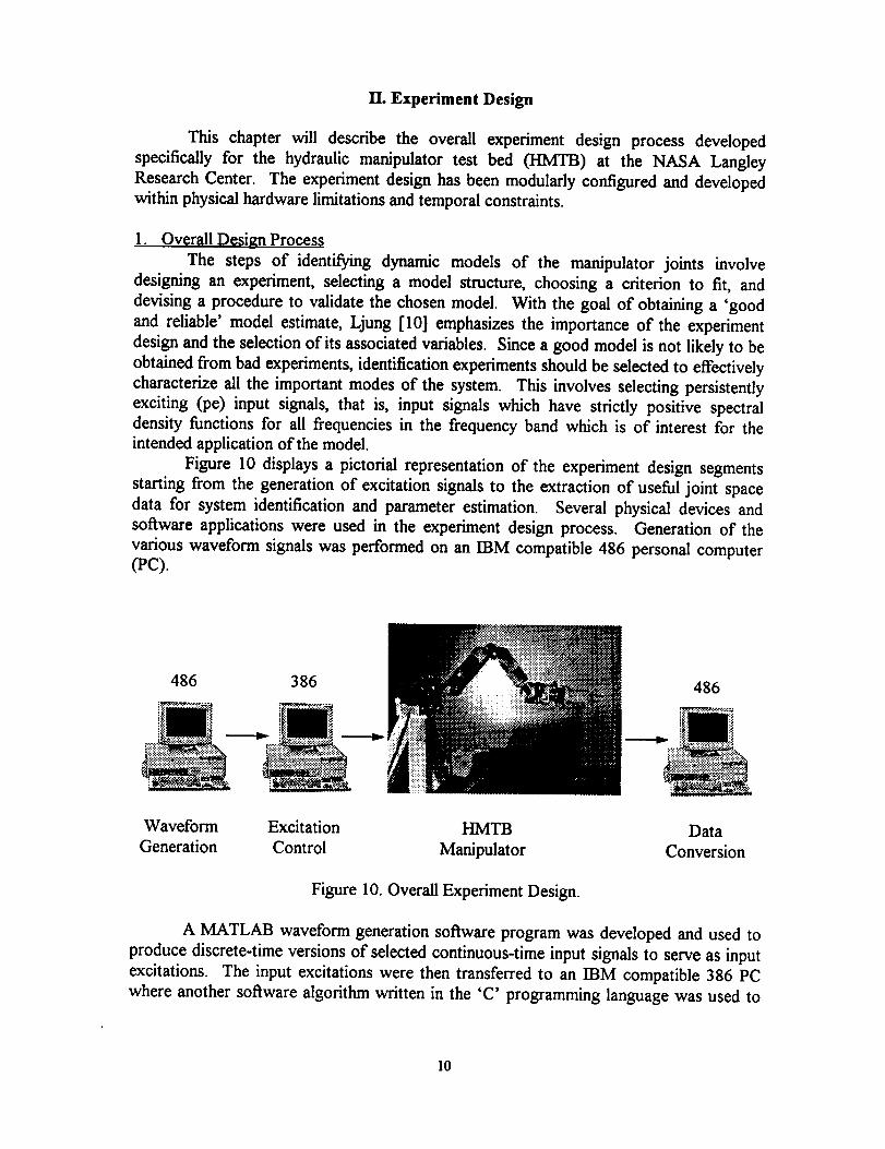
Figure 10 displays a pictorial representation of the experiment design segments
starting from the generation of excitation signals to the extraction of useful joint space
data for system identification and parameter estimation. Several physical devices and
software applications were used in the experiment design process. Generation of the
various waveform signals was performed on an IBM compatible 486 personal computer(PC).
486 386
:::::::::::::::::.::.::..::.... -:i:!:'.':!:_::..!::::.'>.:::::._:
486
_._._:::_:!:_-'.%::i:78_:_;
Waveform Excitation
Generation ControlHMTB Data
Manipulator Conversion
Figure 10. Overall Experiment Design.
A MATLAB waveform generation software program was developed and used to
produce discrete-time versions of selected continuous-time input signals to serve as input
excitations. The input excitations were then transferred to an IBM compatible 386 PC
where another sot_ware algorithm written in the 'C' programming language was used to
10
modulatevarious waveform parameters and to channel the input excitations to specified
joints of the HMTB manipulator. While the HMTB manipulator arm responded to the
input excitations, a data acquisition program written in the Ada programming language
was used to extract joint data from the 1553 bus and to record the data to the HMTB
Control Computer. This data includes the actual input/output time history from each joint.
The recorded 1553 data file was then converted to an ASCII flat file format using an
additional algorithm developed using the Matlab language. The ASCII flat file containing
input/output time histories was then used for nonparametric and parametric analysis.
Prior to the identification experiments, assumptions were made as to the model
form and bandwidth of the open-loop dynamics for each joint. First, a PD control model
with feedforward torque was assumed for each joint. This assumption was based on
analytical models of the flight arm and partial documentation for the ground-based
manipulator. Because of the size of the HMTB manipulator as well as its intended
purpose, the bandwidth for each joint was assumed to correspond to astronaut response
times (3 to 5 Hertz). Due to this assumption, all input excitations used in this
identification were limited to 10 Hertz to satisfy the Nyquist requirement. At least a
second order model was expected due to proportional (P) and derivative (D) components
initially assumed for each PD control loop. The following sections will provide more
detail on the experiment design segments.
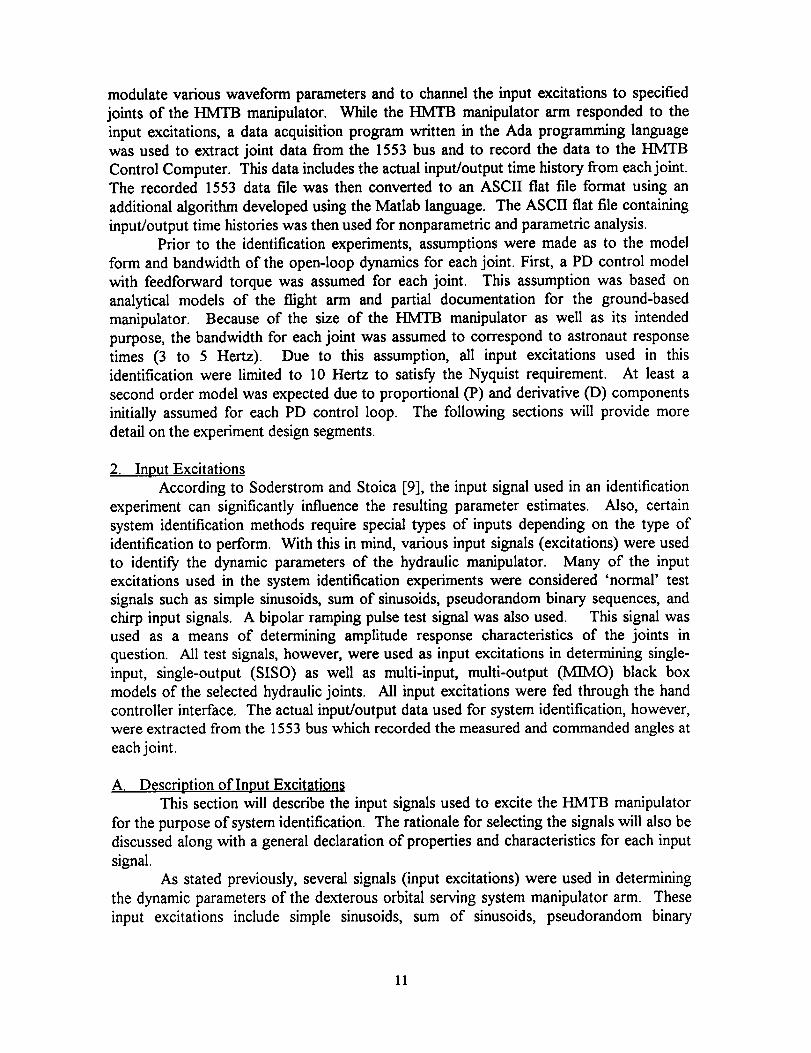
2. Input Excitations
According to Soderstrom and Stoica [9], the input signal used in an identification
experiment can significantly influence the resulting parameter estimates. Also, certain
system identification methods require special types of inputs depending on the type of
identification to perform. With this in mind, various input signals (excitations) were used
to identify the dynamic parameters of the hydraulic manipulator. Many of the input
excitations used in the system identification experiments were considered 'normal' test
signals such as simple sinusoids, sum of sinusoids, pseudorandom binary sequences, and
chirp input signals. A bipolar ramping pulse test signal was also used. This signal was
used as a means of determining amplitude response characteristics of the joints in
question. All test signals, however, were used as input excitations in determining single-
input, single-output (SISO) as well as multi-input, multi-output (MIMO) black box
models of the selected hydraulic joints. All input excitations were fed through the hand
controller interface. The actual input/output data used for system identification, however,
were extracted from the 1553 bus which recorded the measured and commanded angles at
each joint.
A. Description of Input Excitations
This section will describe the input signals used to excite the HMTB manipulator
for the purpose of system identification. The rationale for selecting the signals will also be
discussed along with a general declaration of properties and characteristics for each input
signal.
As stated previously, several signals (input excitations) were used in determining
the dynamic parameters of the dexterous orbital serving system manipulator arm. These
input excitations include simple sinusoids, sum of sinusoids, pseudorandom binary
11

sequences, bipolar ramping pulses, and chirp signals. Each signal was used to excite three
joints (shoulder yaw, shoulder pitch, and elbow pitch) of the HMTB arm. Modulation of
signal parameters will be discussed later.
Good identification experiments provide informative data by which different
models can be discriminated within an intended model set. To provide this informative
data, persistently exciting (pe) input signals must be selected [ 10]. An input signal u(n) is
said to be pe of order m if the spectral density O(w) is not equal to zero for at least m
points in the interval -a" < w < tr for discrete-time systems. With the spectral density
O(w) defined as the discrete Fourier transform of the correlation function, that is,
1 f. )e-*_O(w) = _ R_(r , (2.1)2/r ,__
it has also been determined that u(n) is pe of order m if the limit of the autocorrelation
function exists, that is,
R,,(r)= lim 1"-,= N Z u(t + r),, _(t) (2.2)
t=l
and the autocorrelation matrix
I R_(0) g_(1) .. R=(n-1)]
R,,(n)= /R_(.-1) R_(0) " J (2.3)/LRo(i.n) .... g,.io)
is nonsingular [ 10].
exciting of all orders [9].
3
2
The white noise signal e(t), simulated in Figure 11, is persistently
White Noise
1
0
-1
-2
-30i I I
20 40 60|
80 100
Figure 11. Simulated White Noise.
12
Sinusoidal Input
For the most simple input excitation, a sinusoid was selected to provide frequency
response characteristics at a particular frequency and phase shift. Because of its
simplicity, this signal was selected primarily for test purposes, that is, to determine if the
joint in question was indeed responding to the input signal. Using a sinusoidal input
u(t) = a sin( wt ), (2.4)
the steady state output, assuming the system is linear, will become
Y(O = b sin( wt + _ ) (2.5)
where
b=aIa( )l, and (2.6)
= arg[G(/w)]. (2.7)
The phase # for this signal will be negative, else the system is responding with no input.
It should be noted that this input excitation is rather sensitive to disturbances (noise) and
could be improved by repeating the sinusoid at a number of frequencies to obtain a
graphical representation of the transfer function G(/w) as a function ofw.
Sum of Sinusoids
A sum of sinusoids provides a slight variation from the simple sinusoid by
increasing the number of sinusoidal inputs with distinct frequency components which
yields a greater bandwidth (BW) in the frequency domain. This type of input is used
primarily in transfer function analysis. The discrete-time sum of two sinusoids input
expressed mathematically as
u(n) = al sin( win ) + a2 sin( w_n ) (2.8)
where
0 < w_ < w2 < 2x (2.9)
was used in the identification experiments, though the number of sinusoids need not be
limited to two. As a general rule, the input u(n) will be pe of order 2m where m is the
number ofsinusoids in the sum [9]. Therefore, to identify a fourth order system, only two
sinusoids need be summed. The power spectral density for an infinite sequence of the sumof sinusoids is
2
[8(w-w,)+8(w+w,)] + a2= T T [a(w- w2)+ + ] (2.10)
13
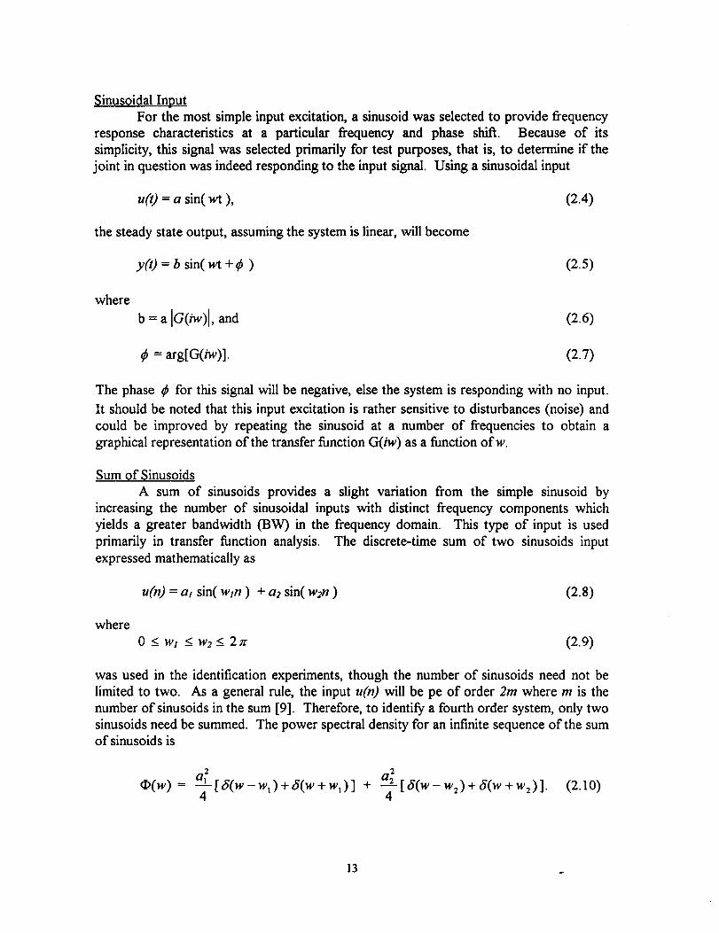
Sincethereare exactly m=4 nonzero points in the interval (-n', n" ], the actual input signal
u(n) is said to be pe of order at least 4. Figure 12 displays a sum of two sinusoids signal
where a_ = 1.0, a2 = 1.0, wz = 0.02a', and w2 = 0.08n-. Figure 13 displays a plot of the
estimated power spectral density of the sum of sinusoids signal. Plots of the actual
excitation signals used for system identification of the HMTB joints are shown in the next
chapter along with their power spectral densities.
For notation purposes, the term 'sum of sinusoids at 10 Hertz' used in this thesis
means that the highest frequency componentJ_ of the given conditionJ_ = 4fi for the sum
of two sinusoids input will be equal to 10 Hz. This also implies that the lower frequency
componentfi is equal to 2.5 Hz. For all sum of two sinusoids experiments performed on
the HMTB joints, the arbitrarily selected condition_ = 4fi will hold.
2
1.5
1
0.5
0
-0.5
-1
-1.5
WaveformPlot
20 40 60 80 100
Figure 12. Sum ofSinusoids.
60 . PSD of Sum of S!nusoids ,...........::...........::...........4or''',_ .............. .,...........:............,...........
Power 30 r - ..... 1---i ........... i ........... ; ........... i ...........
Spec 20 l-........ I_-i ........... i ........... i ........... i ...........Mag I f I ,_ : : :
(0B> ....i...........i...........i-10 i " ' ........ : "'" : ...........
-30_ 5 10 15 20 25Freauencv
Figure 13. PSD of Sum of Sinusoids.
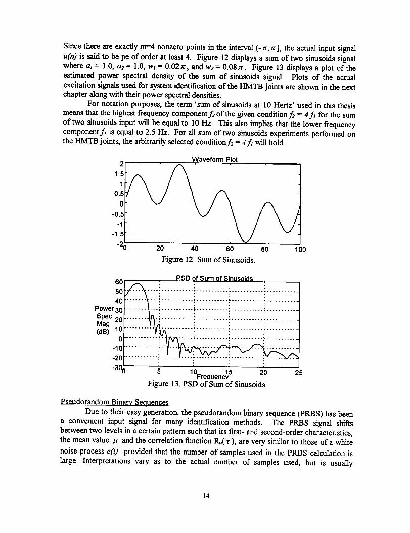
Pseudorandom Binary_ Sequences
Due to their easy generation, the pseudorandom binary sequence (PRBS) has been
a convenient input signal for many identification methods. The PRBS signal shifts
between two levels in a certain pattern such that its first- and second-order characteristics,
the mean value _ and the correlation function 1%(r), are very similar to those of a white
noise process e(t) provided that the number of samples used in the PRBS calculation is
large. Interpretations vary as to the actual number of samples used, but is usually
14
experimentdependent.Therefore,this type of input signal applies itself well to determine
correlation effects of various system parameters. Since the PRBS is band-limited and is
periodic, it differs from a true white noise process. The PRBS is said to be pe of order
equal to its period. Soderstrom and Stoica [9] indicate that in most cases the period of a
PRBS is chosen to be of the same order as the number of samples in the experiment, or
larger. Figure 14(a) depicts the PRBS signal. Its mathematical expression can be realized
as
u(O = (Cl + C2) + (C1 - C_)sign(R(r ) u(t-l) + w(t) ) (2.11)
where
C_ and C2 are permissible binary levels,
R( r ) is the covariance function, and
w(t) is a simulated white noise process.
Figure 14(b) displays the power spectral density of the PRBS input signal.
1.5 W_v_.fnrm pint
1
0.5
0
-0.5
-1
-1_50
L_
4'o do 8'0 100
PSD of PRBS
5o ......... i....................iii.!!.. iii ii
Power 40Spect
Mag ii I il
(dB)
,
100 5 1Q_ 15 20 25Prequencv
Figure ]4. (a) Pseudorandom Binary Sequence (b) PSD of PRBS.
15
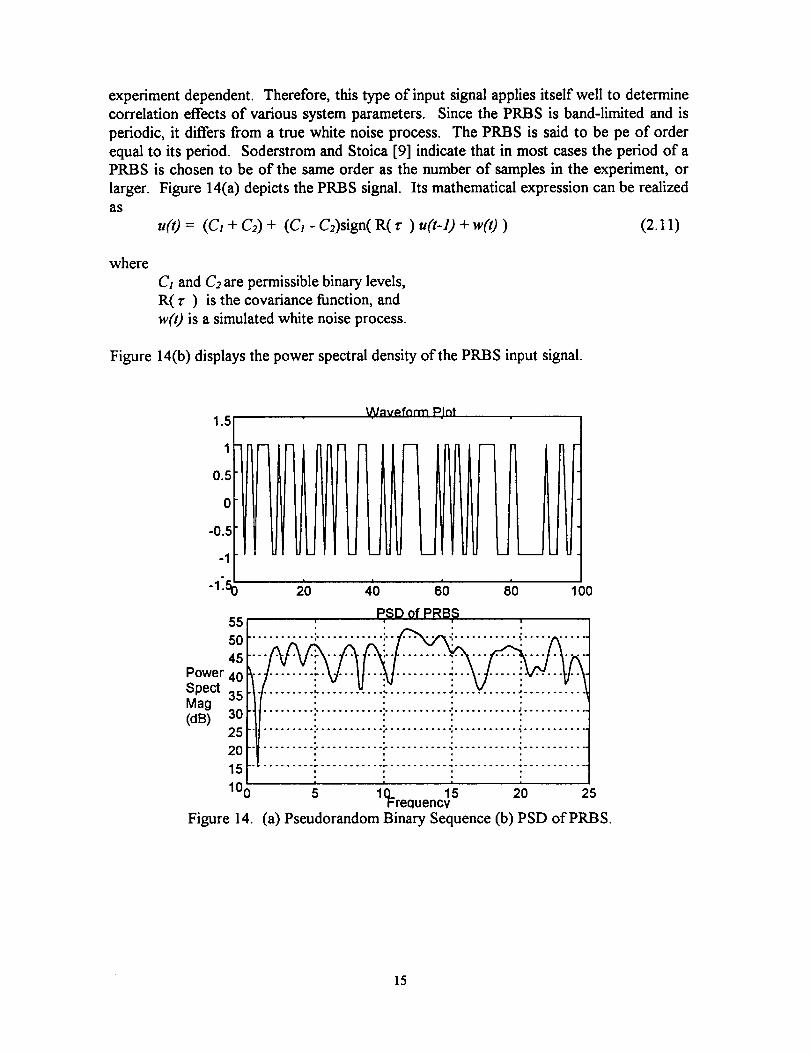
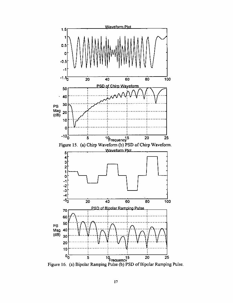
Chirp_ Signal
Chirp is a technique invented by B. M. Oliver at Bell Labs in which signals are
represented by a rapid up or down sweep in frequency [13]. Chirp signals (sine sweeps)
have been used for both radar and communication applications. This waveform was
chosen as an input signal because of its selectable frequency range. Chirp signals have
been known to produce regions with low power spectrum [14]. For this reason, Franklin,
Powell, and Workman [14] describe an expression for a chirp signal that does not have
low power spectrum in the desired bandwidth. Their chirp waveform is expressed as
rk = Ao+aksin2n'j_k, (2.12)
ak=a,,,,= sat (p---_l sat[-_-I, and (2.13)
where
=Y,,or,+ -A.. ),
N = number of points in the data window,
Ao = constant reference offset adjustment,
a,,,_,= maximum amplitude,
p = fraction of window length for amplitude ramps,
./',t,,,, = starting frequency of chirp, and
./',top = stopping frequency of chirp.
(2.14)
The chirp expression used in the identification experiments of this thesis, however, can be
characterized with the following equation:
u(t) = cos( 2a'(f I +tA) + 2nfot ) (2.15)
where
35 is the starting frequency,
is the ending frequency,
fo is the center frequency, and
A .35.
A chirp waveform is shown in Figure 15(a) having values35 = 1 Hz, fo= 4 Hz, andfh = 2
Hz. The power spectral density of the chirp is shown in Figure 15(b).
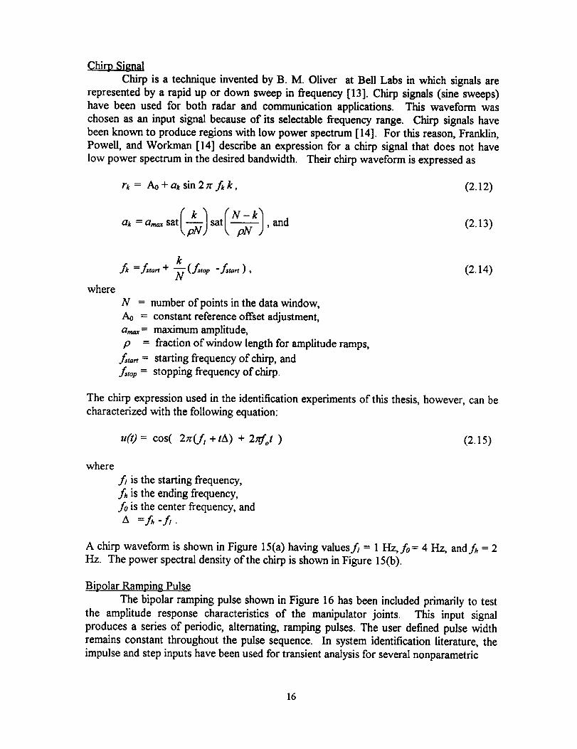
Bipolar Ramping Pulse
The bipolar ramping pulse shown in Figure 16 has been included primarily to test
the amplitude response characteristics of the manipulator joints. This input signal
produces a series of periodic, alternating, ramping pulses. The user defined pulse width
remains constant throughout the pulse sequence. In system identification literature, the
impulse and step inputs have been used for transient analysis for several nonparametric
16
1.5 VVaveform P.Iot
1
0.5
0
-0.5
-1
-1.50 20 40i
80 100
5O
4O
PS 30
Mag(dB) 20
10
0
-lo6
Figure 15.
543
210'
-1-2
-3-4
-50
PSD of Chim Waveform
..........i...........i....• iiii : ii::| I ! I
5 10Frequency5-- . 20 25
(a) Chirp Waveform (b) PSD of Chirp Waveform.
Wnvefnrm Pint
2'0 4'0 6'0 8'0 looPSD of Bioolar Ram )inaPulse
7°1.. i i - i
6o_-\ ......::............::............!..........._............
PSMag_00I_l.__50 .... i......... i............ i ........... ":............
40 i....... i........ ::....... ! .......
(dB) 30 ' " ": ...... i " "i .....
00 5 10._ 15 20 25hreauencv
Figure 16. (a) Bipolar Ramping Pulse (b) PSD of Bipolar Ramping Pulse.
17
identification experiments. This sequence of alternating, ramping pulses will serve as a
test signal for parametric model estimation.
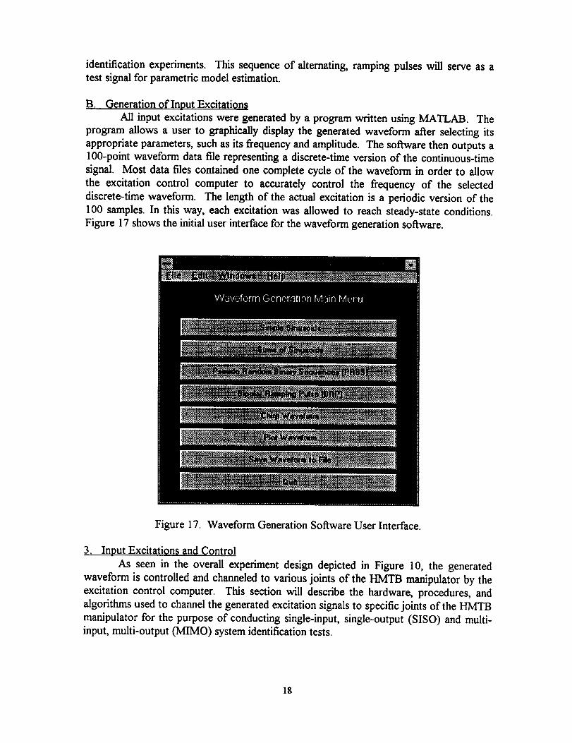
B. Generation 0fInput Excitations
All input excitations were generated by a program written using MATLAB. The
program allows a user to graphically display the generated waveform aiter selecting its
appropriate parameters, such as its frequency and amplitude. The soitwar¢ then outputs a
100-point waveform data file representing a discrete-time version of the continuous-time
signal. Most data files contained one complete cycle of the waveform in order to allow
the excitation control computer to accurately control the frequency of the selected
discrete-time waveform. The length of the actual excitation is a periodic version of the
100 samples. In this way, each excitation was allowed to reach steady-state conditions.
Figure 17 shows the initial user interface for the waveform generation sottwar¢.
Figure 17. Waveform Generation Soi_ware User Interface.
3. Input Excitations and Control
As seen in the overall experiment design depicted in Figure 10, the generated
waveform is controlled and channeled to various joints of the HMTB manipulator by the
excitation control computer. This section will describe the hardware, procedures, and
algorithms used to channel the generated excitation signals to specific joints of the HMTB
manipulator for the purpose of conducting single-input, single-output (SISO) and multi-
input, multi-output (MIMO) system identification tests.
18
A. Single Joint Excitation
The excitation control computer, an IBM 386 PC, was used to perform all system
identification tests. This PC contained the AT-MIO-16 National Instruments data
acquisition board [15]. The AT-MIO-16 applies itself well to various multifunction
analog, digital, and timing applications. In the experiment design, the AT-MIO-16 was
used to convert the discrete-time input waveform to an equivalent frequency modulated
analog signal. This was accomplished by forming a periodic version of each 100-sample
waveform and then outputting the new frequency modulated signal through the digital-to-
analog converter.
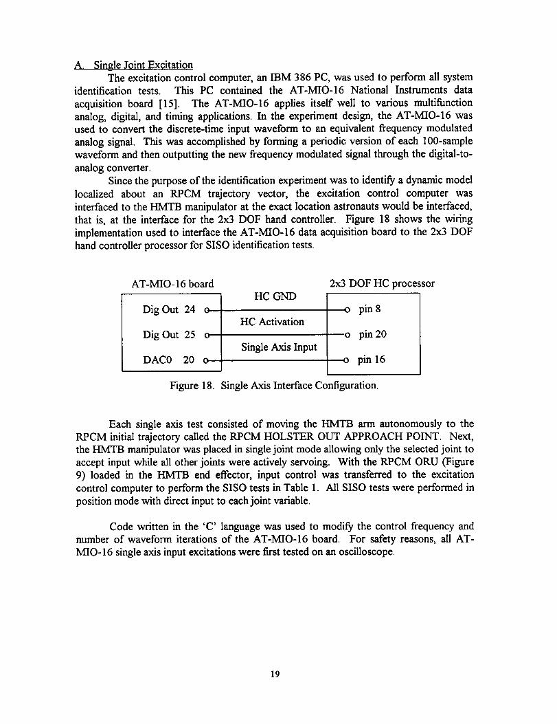
Since the purpose of the identification experiment was to identify a dynamic model
localized about an RPCM trajectory vector, the excitation control computer was
interfaced to the HMTB manipulator at the exact location astronauts would be interfaced,
that is, at the interface for the 2x3 DOF hand controller. Figure 18 shows the wiring
implementation used to interface the AT-MIO-16 data acquisition board to the 2x3 DOF
hand controller processor for SISO identification tests.
AT-MIO- 16 board
Dig Out 24 o
Dig Out 25 o
DAC0 20 o
HC GND
HC Activation
Single Axis Input
2x3 DOF HC processor
o pin 8
o pin 20
o pinl6
Figure 18. Single Axis Interface Configuration.
Each single axis test consisted of moving the HMTB arm autonomously to the
RPCM initial trajectory called the RPCM HOLSTER OUT APPROACH POINT. Next,
the HMTB manipulator was placed in single joint mode allowing only the selected joint to
accept input while all other joints were actively servoing. With the RPCM ORU (Figure
9) loaded in the HMTB end effector, input control was transferred to the excitation
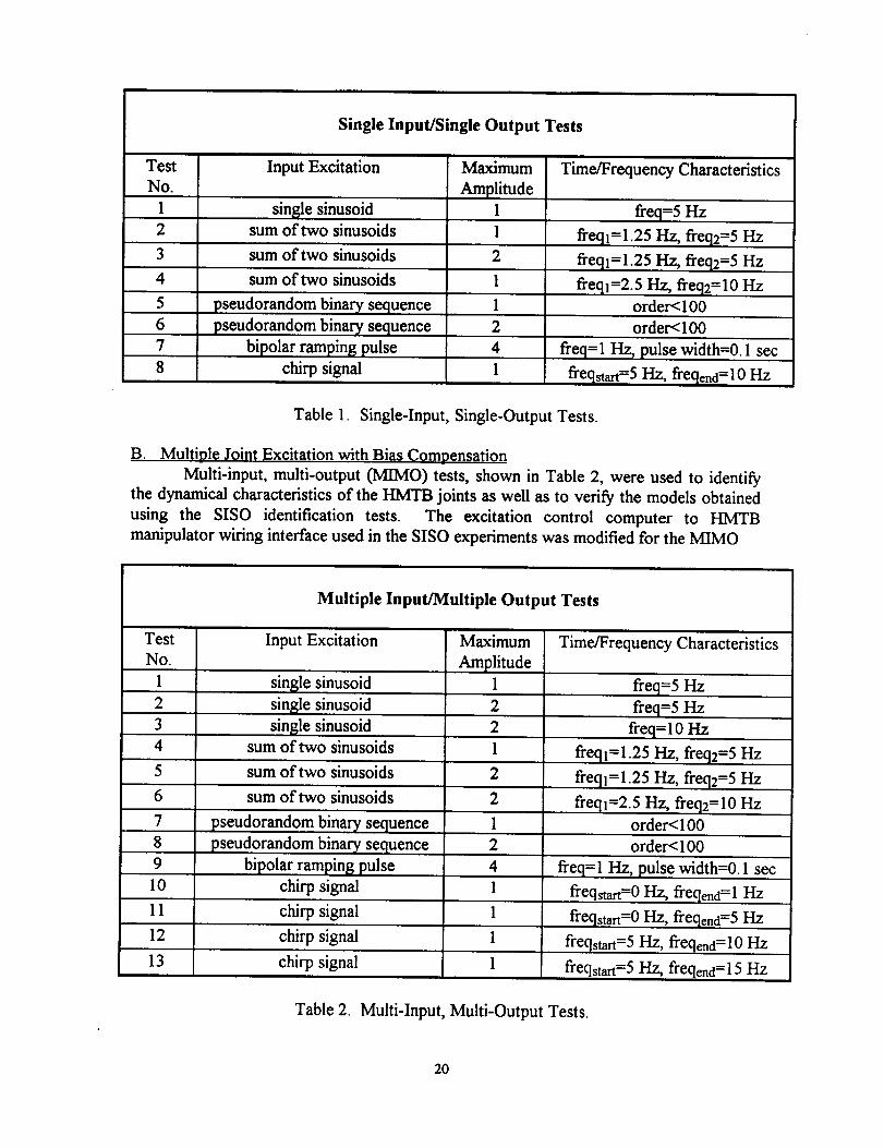
control computer to perform the SISO tests in Table 1. All SISO tests were performed in
position mode with direct input to each joint variable.
Code written in the 'C' language was used to modify the control frequency and
number of waveform iterations of the AT-MIO-16 board. For safety reasons, all AT-
MIO-16 single axis input excitations were first tested on an oscilloscope.
19
Single Input/Single Output Tests
Test
No.
1
2
3
4
5
6
7
Input Excitation
single sinusoid
sum of two sinusoids
sum of two sinusoids
sum of two sinusoids
pseudorandom binary sequence
pseudorandom binary sequence
bipolar ramping pulse
chirp signal
Maximum
Amplitude
1
Time/Frequency Characteristics
freq=5 Hz
1
2 order<100
4
freql=1.25 Hz, freq2=5 Hz
freql=l.25 Hz, freq2=5 Hz
freql=2.5 Hz, freq2=10 Hzorder< 100
freq=l I-Iz, pulse width=0.1 sec
freqstart=5 Hz, freqend=10 Hz
Table 1. Single-Input, Single-Output Tests.
B. Multiple Joint Excitation with Bias Compensation
Multi-input, multi-output (MIMO) tests, shown in Table 2, were used to identify
the dynamical characteristics of the HM joints as well as to verify the models obtained
using the SlSO identification tests. The excitation control computer to HMTB
manipulator wiring interface used in the SlSO experiments was modified for the MIMO
Multiple Input/Multiple Output Tests
Test
No.
1
2
3
4
5
6
7
10
11
12
13
Input Excitation
sinsle sinusoid
single sinusoid
sinl_le sinusoid
sum of two sinusoids
Maximum
Amplitude1
pseudorandom binary sequence
pseudorandom binary sequence
bipolar ramping pulse
chirp signal
2
2
1
sum of two sinusoids 2
sum of two sinusoids 2
1
chirp signal
chirp signal
chirp signal
Time/Frequency Characteristics
freq=5 Hz
freq=5 Hz
freq=l 0 Hz
freql=1.25 Hz, freq2=5 Hz
freql=1.25 Hz, freq2=5 Hz
freq !=2.5 Hz, freq2 = 10 Hz
order<100
order<100
freq=l FIz, pulse width=O. 1 sec
freqstart=O Hz, freqend=l Hz
freqstart=0 Hz, freqencl=5 Hz
freqstart=5 Hz, freqend=l 0 Hz
freqstart=5 Hz, freqend=l 5 Hz
Table 2. Multi-Input, Multi-Output Tests.
20
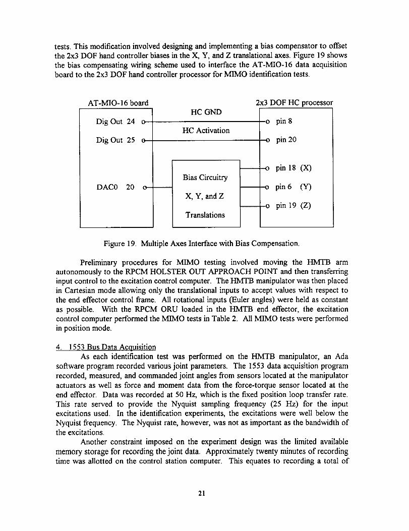
tests. This modification involved designing and implementing a bias compensator to offset
the 2x3 DOF hand controller biases in the X, Y, and Z translational axes. Figure 19 shows
the bias compensating wiring scheme used to interface the AT-MIO-16 data acquisition
board to the 2x3 DOF hand controller processor for MIMO identification tests.
AT-MIO- 16 board
Dig Out 24 o
Dig Out 25 o
DAC0 20 o
HC GND
HC Activation
Bias Circuitry
X, Y, and Z
Translations
2x3 DOF HC processor
o pin 8
o pin 20
o pinl8 (X)
• o pin 6 (Y)
o pinl9 (Z)
Figure 19. Multiple Axes Interface with Bias Compensation.
Preliminary procedures for MIMO testing involved moving the HMTB arm
autonomously to the RPCM HOLSTER OUT APPROACH POINT and then transferring
input control to the excitation control computer. The HMTB manipulator was then placed
in Cartesian mode allowing only the translational inputs to accept values with respect to
the end effector control frame. All rotational inputs (Euler angles) were held as constant
as possible. With the RPCM ORU loaded in the HMTB end effector, the excitation
control computer performed the MIMO tests in Table 2. All MIMO tests were performed
in position mode.
4. 1553 Bus Data Acquisition
As each identification test was performed on the HMTB manipulator, an Ada
software program recorded various joint parameters. The 1553 data acquisition program
recorded, measured, and commanded joint angles from sensors located at the manipulator
actuators as well as force and moment data from the force-torque sensor located at the
end effector. Data was recorded at 50 Hz, which is the fixed position loop transfer rate.
This rate served to provide the Nyquist sampling frequency (25 Hz) for the input
excitations used. In the identification experiments, the excitations were well below the
Nyquist frequency. The Nyquist rate, however, was not as important as the bandwidth ofthe excitations.
Another constraint imposed on the experiment design was the limited available
memory storage for recording the joint data. Approximately twenty minutes of recording
time was allotted on the control station computer. This equates to recording a total of
21

five experiment tests per run. After each set of five tests, the recorded files would have to
be transferred to another computer to provide memory for another set of tests.
5. 1553 Bus Format to ASCII Conversion
The final segment of the experiment design involved converting the 1553 recorded
data file to an ASCII flat file format. This task was performed by a MATLAB conversion
program. The conversion program extracted measured and commanded joint data fromthe 1553 formatted data file to be identified and saved this data in an ASCII flat file format
to be used for nonparametric and parametric analysis.
22
Ill. Nonparametric Model Estimation
As a precursor to parametric identification, nonparametric methods are used first
to extract characteristics of the unknown system which provides information in how to
apply various parametric techniques. This chapter will show results of applying frequency,
correlation, and spectral analysis techniques to the shoulder yaw, shoulder pitch, and
elbow pitch joints of the HMTB manipulator. The results will help determine appropriate
parametric model structures for the next chapter.
1. Procedure Description and Rationale
Nonparametric model estimation involves determining a system's characteristics
from Bode plots and plots of input/output cross-correlation. Though sufficient,
nonparametric methods give only moderately accurate models. For time domain
nonparametric analysis, the impulse response and the step response are both useful in
determining some basic control related characteristics of a system such as delay time,
static gain and dominating time constants. Frequency domain techniques provide
information such as the estimated transfer function, the bandwidth of a system, and a
system's phase characteristics. The techniques employed in this investigation include
transfer function analysis, correlation analysis, and spectral analysis.
Transfer function analysis was used to determine the frequency response of the yet
to be identified system. This information helped to determine the frequency range of the
input excitations to be used in the identification experiments. The frequency response
approach was performed by applying a sum of sinusoidal inputs to the system and then
recording the input/output time histories for each joint. Autocorrelation and cross-
correlation functions were first computed from the data and then transformed to power
spectral density and cross-power spectral density estimates, respectively. Spectral
estimates were smoothed and averaged by using a Hamming window with the lag length
approximately equal to a tenth of the number of data points. The estimated transfer
function for each joint was computed as the ratio of the cross-power spectrum to the input
power spectrum. Each joint's transfer function estimate was represented in the form of
Bode plots.
Correlation analysis techniques were employed to provide information on the
degree of linear dependence of a system's parameters, that is, how well future values of
the data can be predicted based on past observations. Correlation analysis is usually based
on white noise or any input signal that is independent of the disturbances. A distinct
advantage of correlation techniques is its insensitivity to additive noise on the output [9].
Spectral analysis, a very versatile nonparametric technique, used various
persistently exciting input signals to yield spectral estimates of the system. The spectral
density or spectrum is a frequency domain function used to measure the frequency
distribution of the mean square value of the data. Spectral estimates for each joint were
computed using a Hamming window with the lag length approximately equal to a tenth of
the number of data points.
23
2. Shoulder Yaw Joint
A. Transfer Function Analysis
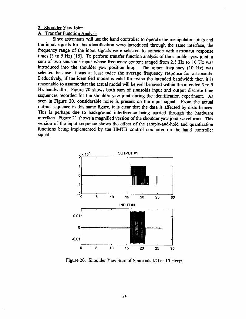
Since astronauts will use the hand controller to operate the manipulator joints and
the input signals for this identification were introduced through the same interface, the
frequency range of the input signals were selected to coincide with astronaut response
times (3 to 5 Hz) [16]. To perform transfer function analysis of the shoulder yaw joint, a
sum of two sinusoids input whose frequency content ranged from 2.5 Hz to 10 Hz was
introduced into the shoulder yaw position loop. The upper frequency (10 Hz) was
selected because it was at least twice the average frequency response for astronauts.
Deductively, if the identified model is valid for twice the intended bandwidth then it is
reasonable to assume that the actual model will be well behaved within the intended 3 to 5
Hz bandwidth. Figure 20 shows both sum of sinusoids input and output discrete time
sequences recorded for the shoulder yaw joint during the identification experiment. As
seen in Figure 20, considerable noise is present on the input signal. From the actual
output sequence in this same figure, it is clear that the data is affected by disturbances.
This is perhaps due to background interference being carded through the hardware
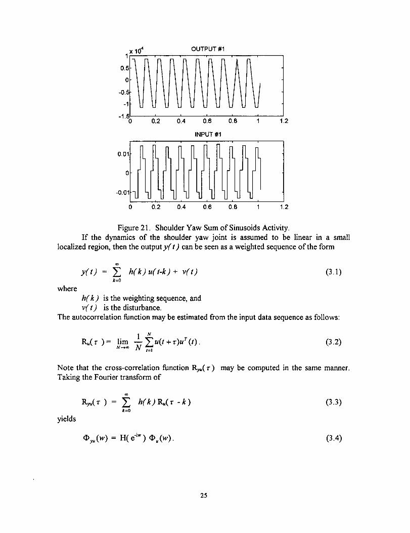
interface. Figure 21 shows a magnified version of the shoulder yaw joint waveforms. This
version of the input sequence shows the effect of the sample-and-hold and quantization
functions being implemented by the HMTB control computer on the hand controllersignal.
2 xl_
1
0
-1
-20
OUTPUT #1
llllll/III I I I I
5 10 15 20 25 30
INPUT #1
0 5 10 15 20 25 30
Figure 20. Shoulder Yaw Sum of Sinusoids I/O at 10 Hertz.
24
xlO"1
0.50 l-0.5
-1
-1.50 012
0.01
OUTPUT #1
'i' 016 '0,4 0.8
, i
'l lI i
0.2 0.4
JI
1
INPUT #1i
i i
0.6 0.8
1.2
-0.01 "1.i
0 1 1.2
Figure 21. Shoulder Yaw Sum of Sinusoids Activity.
If the dynamics of the shoulder yaw joint is assumed to be linear in a small
localized region, then the output y(t) can be seen as a weighted sequence of the form
where
y(t) = _ h(k) u(t-k) + v(t) (3.1)k=0
h(k) is the weighting sequence, and
v(t) is the disturbance.
The autocorrelation function may be estimated from the input data sequence as follows:
R.(r)= lim --1 N,,-_ N _"(t + _).T(t). (3.2)t=l
Note that the cross-correlation function R_(r) may be computed in the same manner.
Taking the Fourier transform of
Ry,(r ) = _ h(k)I_(r -k) (3.3)k=0
yields
_.,(w) = H( e"i* ) O.(w). (3.4)
25

The estimated transfer function is computed as
H(e "i*) = t_,(w) / t_=(w). (3.5)
The discrete-time transfer function estimate for the sum of sinusoids data sequence isshown in Figure 22.
10 0
10 -_
10 .2
10 .310 0
2OO
AMPLITUDE PLOT, input # 1 output # 1-i
..... I ....... =
101 10 2 103
0
pha_O
-400 .......100 101 10 2 10 3
frequency (rad/sec)
Figure 22. Shoulder Yaw Transfer Function Estimate.
Graphical interpretation of this transfer function yields a gain less than one for the
entire bandwidth with a low frequency cutoff at approximately w= 6 rad/sec. The
negative slope slightly above the break frequency indicates a second-order system until
approximately 10 rad/sec. The rest of the graph shows additional resonances and
disturbances of the system above 10 rad/sec.
B. Correlation Analy_;is
Correlation analysis techniques were applied to the shoulder yaw joint to provide
information on the degree of linear dependence of the input and output of the joint.
Correlation analysis is usually based on white noise or any input signal that is independent
of the disturbances. For this reason, a pseudorandom binary sequence (PRBS) was used
to excite the joint. PRBS signals simulate white noise statistical properties for the purposeof nonparametric identification. The one difference between PRBS and white noise is its
periodicity. The mathematical PRBS expression has already been shown (2.11). Figure
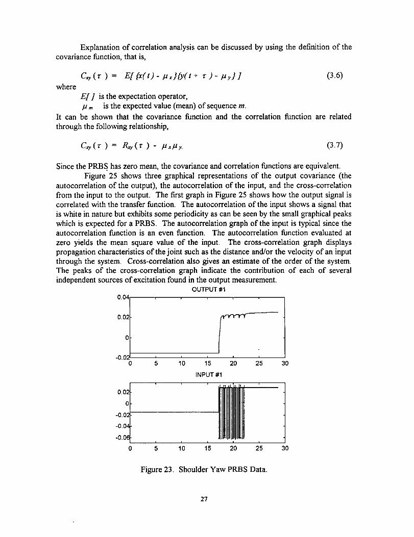
23 shows the entire input/output sequence of the PRBS input signal applied to the
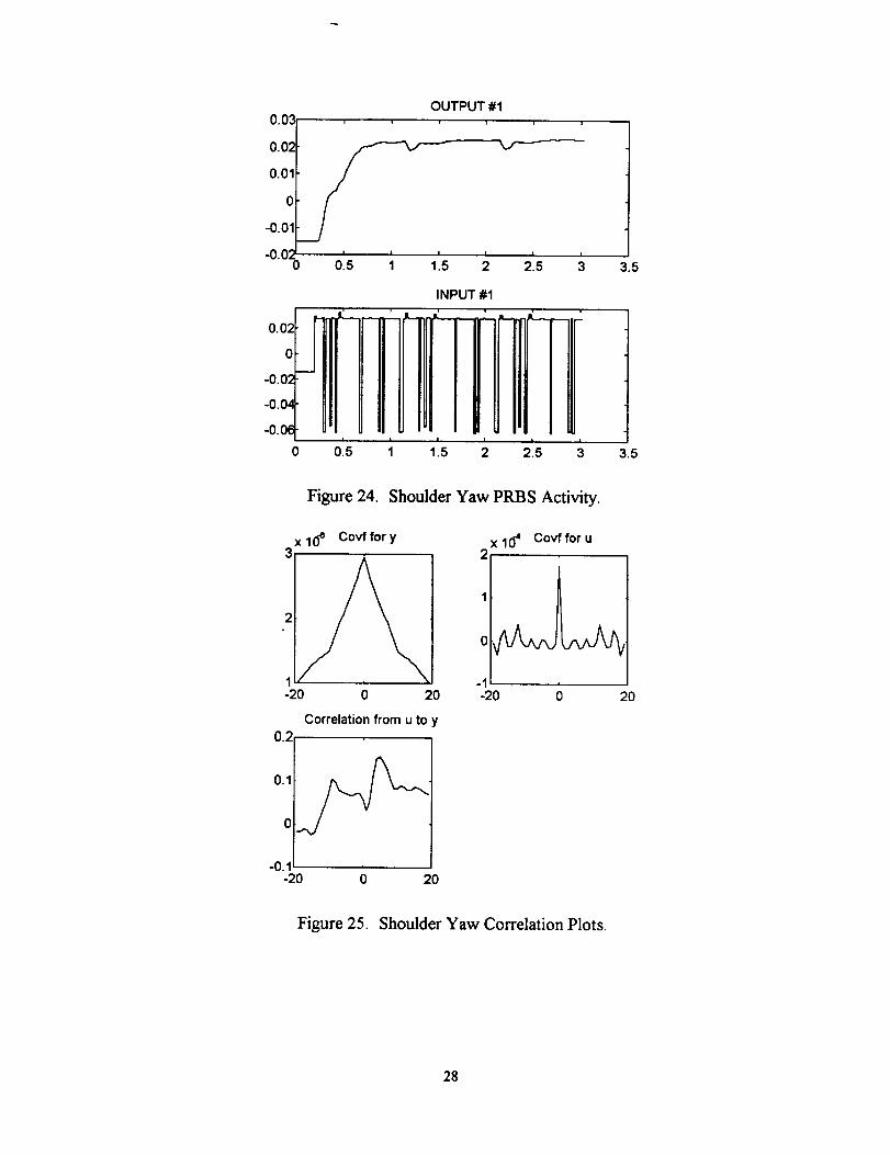
shoulder yaw joint during the identification experiment. Figure 24 shows a magnified
version of the PRBS shoulder yaw joint activity.
26
Explanation of correlation analysis can be discussed by using the definition of the
covariance function, that is,
C_(t ) = E[{x(t)- lZx}{y(t+ t )- lZy}] (3.6)
where
IS[] is the expectation operator,
/z m is the expected value (mean) of sequence m.
It can be shown that the covariance function and the correlation function are related
through the following relationship,
Cxy(r ) = R_v(r ) - ltx/.ty. (3.7)
Since the PRBS has zero mean, the covariance and correlation functions are equivalent.
Figure 25 shows three graphical representations of the output covariance (the
autocorrelation of the output), the autocorrelation of the input, and the cross-correlation
from the input to the output. The first graph in Figure 25 shows how the output signal is
correlated with the transfer function. The autocorrelation of the input shows a signal that
is white in nature but exhibits some periodicity as can be seen by the small graphical peaks
which is expected for a PRBS. The autocorrelation graph of the input is typical since theautocorrelation function is an even function. The autocorrelation function evaluated at
zero yields the mean square value of the input. The cross-correlation graph displays
propagation characteristics of the joint such as the distance and/or the velocity of an input
through the system. Cross-correlation also gives an estimate of the order of the system.
The peaks of the cross-correlation graph indicate the contribution of each of several
independent sources of excitation found in the output measurement.OUTPUT #1
0.04
0.02
-0.020 30
0.02
0
-0.02
-0.0_
-0.0t
0
,
I I I I I
5 10 15 20 25
INPUT #1
[ II al II II I
i[l[lllilllI I I I I
5 10 15 20 25 30
Figure 23. Shoulder Yaw PRBS Data.
27
0.03
0.02
0.01
0
-0.01
-0.02 t0
OUTPUT #1i i _ 1 n
I ! Io._ _ 1'_ _ 2s 3
0.02
0
-0.02
-0.04
-0.06
INPUT #1
I I I / I I
0.5 1 1.5 2 2.5 3
3.5
"4
t3.5
Figure 24. Shoulder Yaw PRBS Activity.
xl_ Covffory3
2//\1-20 0
0.2
0.1
-0.1
2O
Correlation from u to y
-20 0 20
xl04 Covfforu2
1
•1 I-20 0 20
Figure 25. Shoulder Yaw Correlation Plots.
28
C. Spectral Analysis
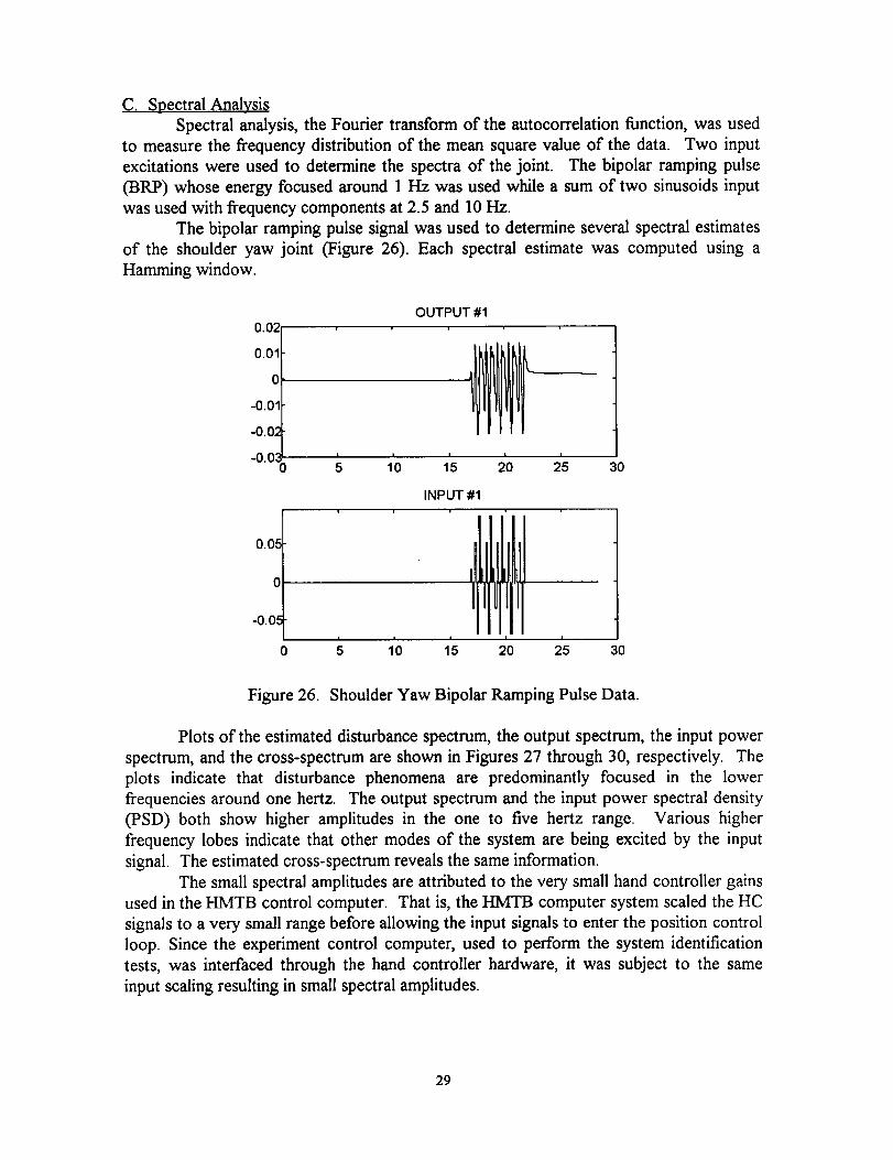
Spectral analysis, the Fourier transform of the autocorrelation function, was used
to measure the frequency distribution of the mean square value of the data. Two input
excitations were used to determine the spectra of the joint. The bipolar ramping pulse
(BRP) whose energy focused around 1 Hz was used while a sum of two sinusoids input
was used with frequency components at 2.5 and 10 Hz.
The bipolar ramping pulse signal was used to determine several spectral estimates
of the shoulder yaw joint (Figure 26). Each spectral estimate was computed using a
Hamming window.
0.0_
0.01
0
-0.01
-0.02
-0.030
OUTPUT #1
I | _ I10 15 0 25 30
INPUT #1
0.05
0
-0.0..=
0I I I I I
5 10 15 20 25 30
Figure 26. Shoulder Yaw Bipolar Ramping Pulse Data.
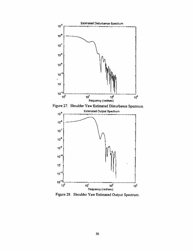
Plots of the estimated disturbance spectrum, the output spectrum, the input power
spectrum, and the cross-spectrum are shown in Figures 27 through 30, respectively. The
plots indicate that disturbance phenomena are predominantly focused in the lower
frequencies around one hertz. The output spectrum and the input power spectral density
(PSD) both show higher amplitudes in the one to five hertz range. Various higher
frequency lobes indicate that other modes of the system are being excited by the input
signal. The estimated cross-spectrum reveals the same information.
The small spectral amplitudes are attributed to the very small hand controller gains
used in the HMTB control computer. That is, the HMTB computer system scaled the HC
signals to a very small range before allowing the input signals to enter the position control
loop. Since the experiment control computer, used to perform the system identification
tests, was interfaced through the hand controller hardware, it was subject to the same
input scaling resulting in small spectral amplitudes.
29
Estimated Disturbance SpectrumlO-5 ...............
lO_
10-7
lo"
lO9
10"1o
10"
10-12lo0
Figure 27.
10 "_ .
lO_
10 -_
10-lo
lO
10"12
10-islOo
Figure 28.
1
- , , . . .
lo1 lO_ i#frequency (radlsec)
Shoulder Yaw Estimated Disturbance Spectrum.
Estimated Output Spectrum
1lO' 1# 1¢
frequency (rad/sec)
Shoulder Yaw Estimated Output Spectrum.
3O
Power Spectral Density (PSD)lO-'
lO_
lO_
10 .7
lO•
10-9 ...........10o 101 102 103
frequency (red/see)
Figure 29. Shoulder Yaw Estimated Input Power Spectrum.
Estimated Cross-SpectrumlO_
lO_
lO_
lff r
10•
10 .9
10.1clOo
....... , ........ i
101 102 103
frequency (red/see)
Figure 30. Shoulder Yaw Estimated Cross-Spectrum.
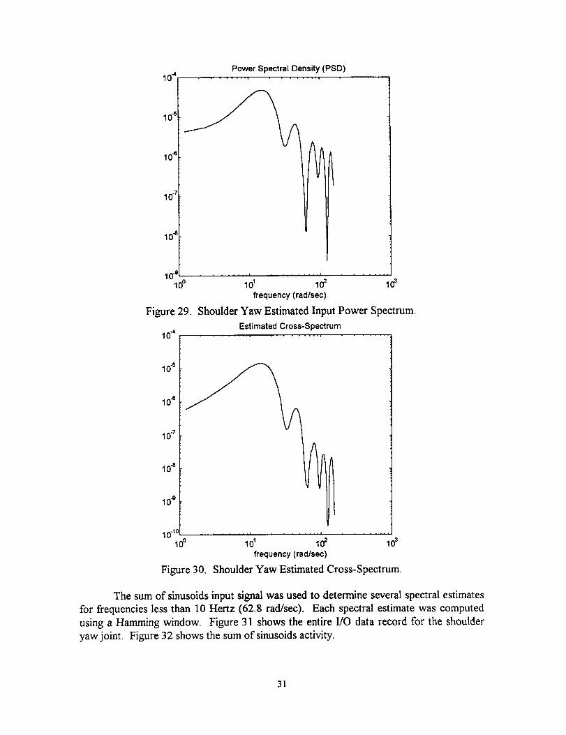
The sum of sinusoids input signal was used to determine several spectral estimates
for frequencies less than 10 Hertz (62.8 rad/sec). Each spectral estimate was computed
using a Hamming window. Figure 31 shows the entire I/O data record for the shoulder
yaw joint. Figure 32 shows the sum of sinusoids activity.
31
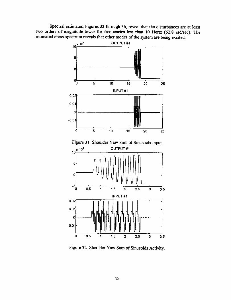
Spectral estimates, Figures 33 through 36, reveal that the disturbances are at least
two orders of magnitude lower for frequencies less than 10 Hertz (62.8 rad/sec). The
estimated cross-spectrum reveals that other modes of the system are being excited.
OUTPUT #1X10⁴I0
I I
"% 5 10 25I I
15 20
0.0;
0.01
........ . . .
-0.01
I
0 5
INPUT #1
I
10 15 20 25
Figure 31. Shoulder Yaw Sum of Sinusoids Input.
I0 x 104 OUTPUT #I
0
I I"% o.s ; 2'.5
0.02
0.01
O_
-0.01
0.5 1
I
115 2
INPUT #1
1.5 2I I
2.5 3 3.5
Figure 32. Shoulder Yaw Sum of Sinusoids Activity.
32
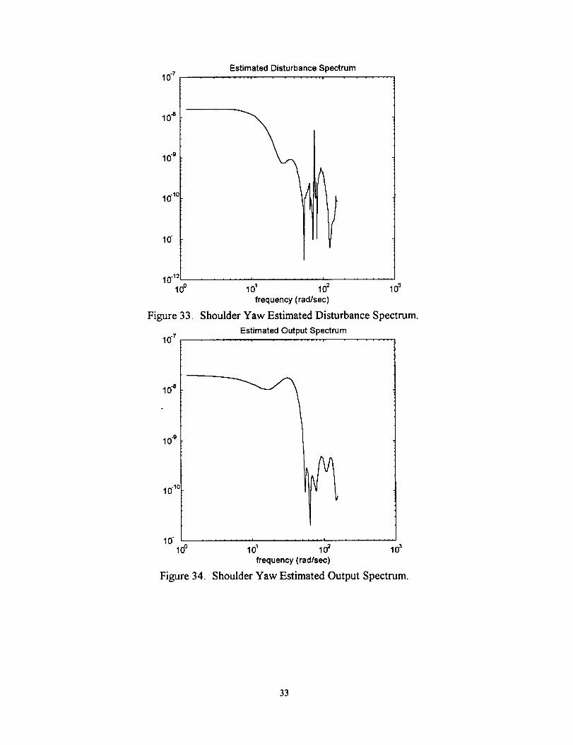
Estimated Disturbance Spectrum10.7 .......
10"8
10g
10"1c
lO
10"1:1o0
Figure 33.
10 .7
101 102 103
frequency (rad/sec)
Shoulder Yaw Estimated Disturbance Spectrum.
Estimated Output Spectrum
lO_
10.9
10-lc
10lO0
Figure 34.
...... , ........ =
lO_ lO2 lO3frequency (rad/sec)
Shoulder Yaw Estimated Output Spectrum
33
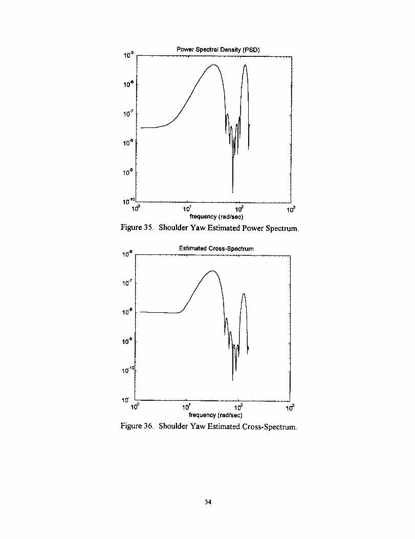
10"s
lO"
10-7
104_
10.9
Power Spectral Density (PSD)
..... , ..= .
101 102 103
frequency (rad/sec)
Figure 35. Shoulder Yaw Estimated Power Spectrum.
Estimated Cross-Spectrum10"e .........
10.7
10"8
10.9
1040
10" ,-, ........ t
10o 101 102 103
frequency (rad/sec)
Figure 36. Shoulder Yaw Estimated Cross-Spectrum.
34
3. Shoulder Pitch and Elbow Pitch Joints
Identical nonparametric procedures performed for the shoulder yaw joint were also
performed for the shoulder pitch and elbow pitch joints. Transfer function analysis for
both joints yielded break frequencies at approximately seven radians per second.
Correlation analysis as applied to both joints yielded two to five delay units from the input
to the output of each joint implying possible system orders. Results from spectral analysis
for each joint indicated that the disturbances were at least an order of magnitude lower
than the output spectrums. Plots and graphs from the nonparametric procedures described
above are displayed in Appendix A. 1 for both shoulder pitch and elbow pitch joints.
4. Nonparametric Conclusions
Transfer function analysis, correlation analysis, and spectral analysis techniques
have been used to determine a crude nonparametric estimation of three HMTB
manipulator joints (shoulder yaw, shoulder pitch, and elbow pitch). The nonparametric
model estimation techniques used in this chapter suggest that parametric models should be
selected to properly model the noise dynamics as well the system's dynamics.
Nonparametric analysis described each joint with minor to moderate process and
measurement disturbances. The plots reveal greater measurement disturbances than
process disturbances. Transfer function analysis of each joint indicates that models need
to be constructed within a 1 to 5 Hz bandwidth.
Errors in the nonparametric estimations may be attributed to several sources:
random errors, bias errors, quantization errors in the experiment design, and choice of
input signal. Random errors are caused by nonlinearities in the system. Bias errors are
due to resolution errors in the spectral density estimates as well as unmeasured inputs that
contribute to the output. Quantization errors are caused by the sample-and-hold function
used in the HMTB control computer when accepting the hand controller input signal.
Velocity limits in the control system also contributed to errors in the estimations. The
experiment design introduced errors on the input measurements with improperly shielded
wires in the experiment control computer interface. When these errors are introduced into
an experiment design, the likelihood of obtaining accurate estimates decreases.
35
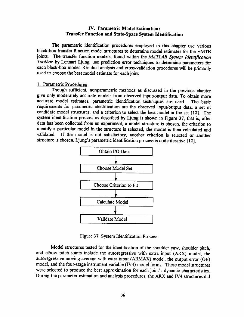
IV. Parametric Model Estimation:
Transfer Function and State-Space System Identification
The parametric identification procedures employed in this chapter use various
black-box transfer function model structures to determine model estimates for the HMTB
joints. The transfer function models, found within the MATIMB System Identification
Toolbox by Lennart Ljung, use prediction error techniques to determine parameters for
each black-box model. Residual analysis and cross-validation procedures will be primarily
used to choose the best model estimate for each joint.
1. Parametric Procedures
Though sufficient, nonparametric methods as discussed in the previous chapter
give only moderately accurate models from observed input/output data. To obtain more
accurate model estimates, parametric identification techniques are used. The basic
requirements for parametric identification are the observed input/output data, a set of
candidate model structures, and a criterion to select the best model in the set [10]. The
system identification process as described by Ljung is shown in Figure 37, that is, after
data has been collected from an experiment, a model structure is chosen, the criterion to
identify a particular model in the structure is selected, the model is then calculated and
validated. If the model is not satisfactory, another criterion is selected or another
structure is chosen. Ljung's parametric identification process is quite iterative [ 10].
Obtain I/O Data
I ooso o oISotI
I oo oC to onto tJ
¢[ Validate Model [
Figure 3 7. System Identification Process.
Model structures tested for the identification of the shoulder yaw, shoulder pitch,
and elbow pitch joints include the autoregressive with extra input (ARX) model, the
autoregressive moving average with extra input (ARMAX) model, the output error (OE)
model, and the four-stage instrument variable (IV4) model forms. These model structures
were selected to produce the best approximation for each joint's dynamic characteristics.
During the parameter estimation and analysis procedures, the ARX and IV4 structures did
36
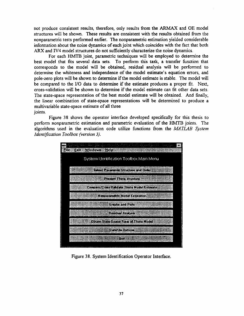
not produce consistent results, therefore, only results from the ARMAX and OE model
structures will be shown. These results are consistent with the results obtained from the
nonparametric tests performed earlier. The nonparametric estimation yielded considerable
information about the noise dynamics of each joint which coincides with the fact that both
ARX and IV4 model structures do not sufficiently characterize the noise dynamics.
For each HMTB joint, parametric techniques will be employed to determine the
best model that fits several data sets. To perform this task, a transfer function that
corresponds to the model will be obtained, residual analysis will be performed to
determine the whiteness and independence of the model estimate's equation errors, and
pole-zero plots will be shown to determine if the model estimate is stable. The model will
be compared to the I/O data to determine if the estimate produces a proper fit. Next,cross-validation will be shown to determine if the model estimate can fit other data sets.
The state-space representation of the best model estimate will be obtained. And finally,
the linear combination of state-space representations will be determined to produce a
multivariable state-space estimate of all three
joints.
Figure 38 shows the operator interface developed specifically for this thesis to
perform nonparametric estimation and parametric evaluation of the HMTB joints. The
algorithms used in the evaluation code utilize functions from the MATLAB System
Identification Toolbox (version 3).
Figure 38. System Identification Operator Interface.
37
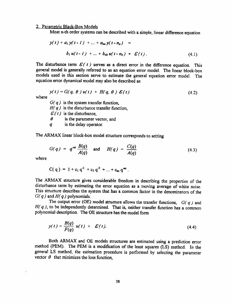
2. Parametric Black-Box Models
Most n-th order systems can be described with a simple, linear difference equation
y(t) + aty(t- 1) +... + a,,y(t-no) =
blu(t-1) +... + b,bu(t-nb) + _(t). (4.1)
The disturbance term ,5"( t ) serves as a direct error in the difference equation. This
general model is generally referred to as an equation error model. The linear block-box
models used in this section serve to estimate the general equation error model. The
equation error dynamical model may also be described as
wherey(t) = G(q, 0 )u(t) + H(q, 0 ) oc(t)
G(q) is the system transfer function,
H(q) is the disturbance transfer function,
_(t) is the disturbance,
0 is the parameter vector, and
q is the delay operator.
(4.2)
The ARMAX linear block-box model structure corresponds to setting
G(q) = q"* B(q) and H(q)- C(q) (4.3)A(q) A(q)
where
C(q) = l+c_q "i +c2q "2 +...+c_q "_.
The ARMAX structure gives considerable freedom in describing the properties of the
disturbance term by estimating the error equation as a moving average of white noise.
This structure describes the system that has a common factor in the denominators of the
G( q ) and H( q ) polynomials.
The output error (OE) model structure allows the transfer functions, G( q ) and
H(q), to be independently determined. That is, neither transfer function has a common
polynomial description. The OE structure has the model form
y(t)- B(q) u(t) + oc'(t). (4.4)F(q)
Both ARMAX and OE models structures are estimated using a prediction error
method (PEM). The PEM is a modification of the least squares (LS) method. In the
general LS method, the estimation procedure is performed by selecting the parameter
vector 0 that minimizes the loss function,
38
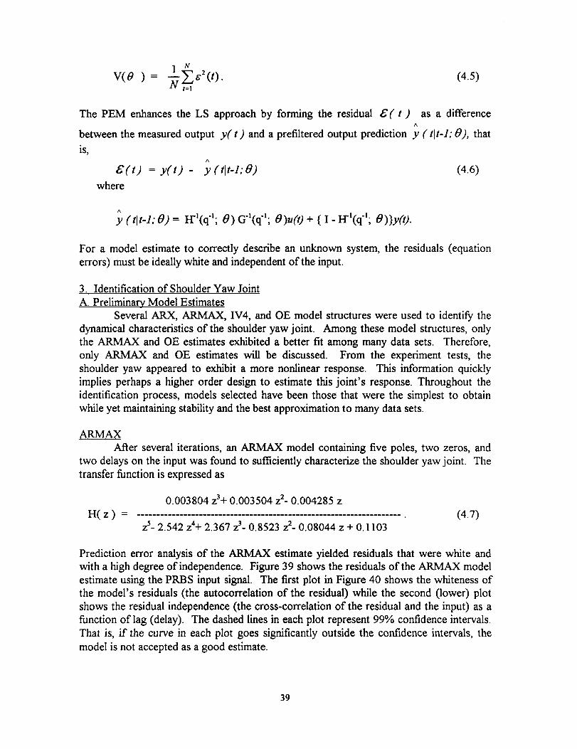
1 N
V(O )- N__62(t). (4.5)t=l
The PEM enhances the LS approach by forming the residual oe( t ) as a differenceA
between the measured output y(t) and a prefiltered output prediction y ( tit-l; 0), that
is,A
C(t) = y(t) - y (tlt-1;O) (4.6)
where
A
y (tit-l; 0) = IT'(q'_; 0) G'_(q"; O)u(O + { I - H'_(q'l; 8)}y(t).
For a model estimate to correctly describe an unknown system, the residuals (equation
errors) must be ideally white and independent of the input.
3. Identification of Shoulder Yaw Joint
A. Preliminary_ Model Estimates
Several ARX, ARMAX, IV4, and OE model structures were used to identify the
dynamical characteristics of the shoulder yaw joint. Among these model structures, only
the ARMAX and OE estimates exhibited a better fit among many data sets. Therefore,
only ARMAX and OE estimates will be discussed. From the experiment tests, the
shoulder yaw appeared to exhibit a more nonlinear response. This information quickly
implies perhaps a higher order design to estimate this joint's response. Throughout the
identification process, models selected have been those that were the simplest to obtain
while yet maintaining stability and the best approximation to many data sets.
ARMAX
After several iterations, an ARMAX model containing five poles, two zeros, and
two delays on the input was found to sufficiently characterize the shoulder yaw joint. The
transfer function is expressed as
0.003804 z3+ 0.003504 z2- 0.004285 z
H(z) ..................................................................... .z 5- 2.542 z4+ 2.367 z 3- 0.8523 z2- 0.08044 z + 0.1103
(4.7)
Prediction error analysis of the ARMAX estimate yielded residuals that were white and
with a high degree of independence. Figure 39 shows the residuals of the ARMAX model
estimate using the PRBS input signal. The first plot in Figure 40 shows the whiteness of
the model's residuals (the autocorrelation of the residual) while the second (lower) plot
shows the residual independence (the cross-correlation of the residual and the input) as a
function of lag (delay). The dashed lines in each plot represent 99% confidence intervals.
That is, if the curve in each plot goes significantly outside the confidence intervals, the
model is not accepted as a good estimate.
39
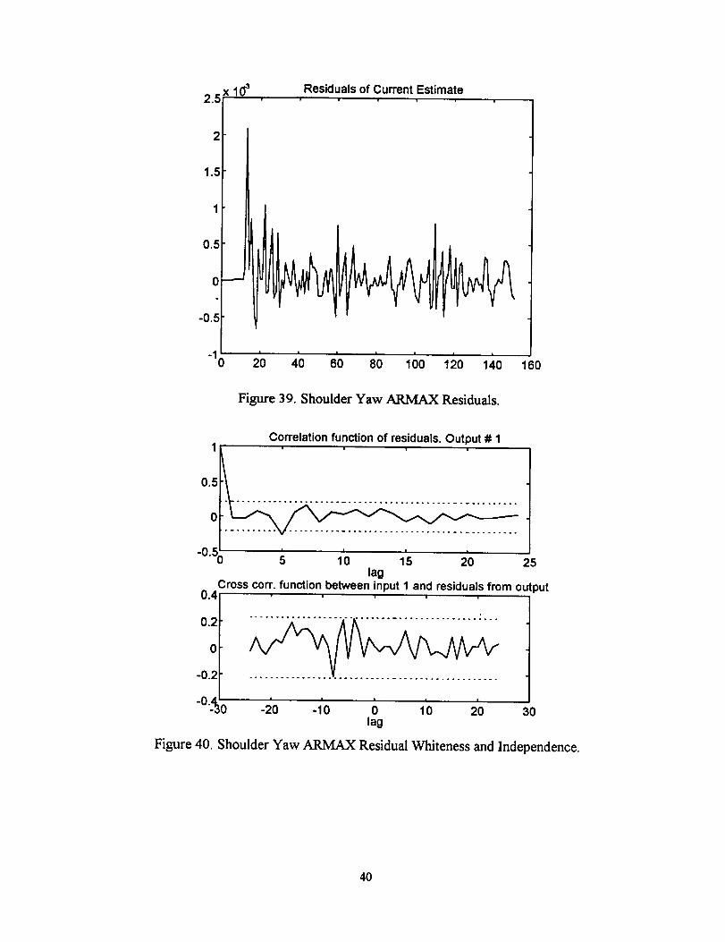
( 103 Residuals of Current Estimate2.5
2
1.5
1
0.5
0
-0.I
-1o 160
J' 4'0 .....20 60 80 100 120 140
Figure 39. Shoulder Yaw ARMAX Residuals.
Correlation function of residuals. Output # 11
0.5_0
s; , , l's '-0. 5 10 20 25lag
Cross corr. function between input 1 and residuals from out )ut0.4
0.20-0.2 ...............................
...4_0 .....-0 -20 -10 0 10 20 30lag
Figure 40. Shoulder Yaw ARMAX Residual Whiteness and Independence.
4O
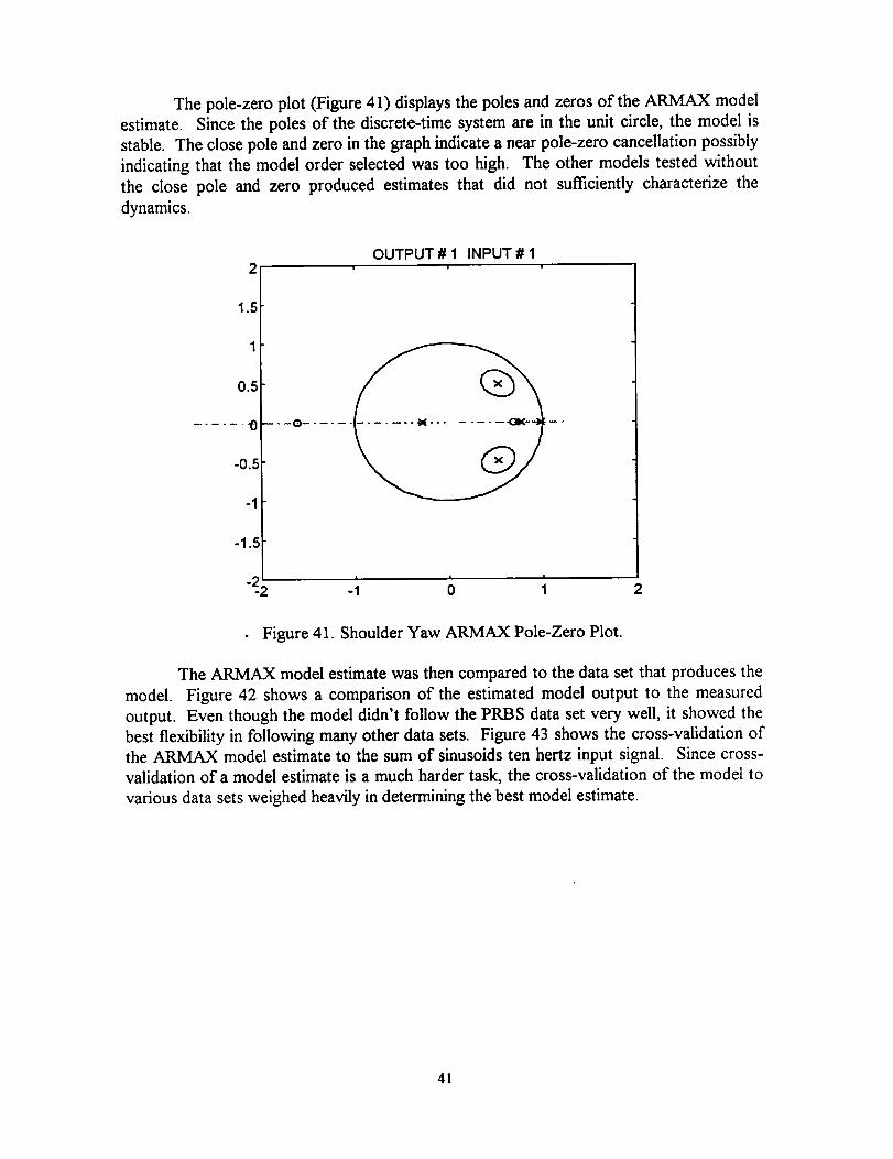
The pole-zero plot (Figure 41) displays the poles and zeros of the ARMAX model
estimate. Since the poles of the discrete-time system are in the unit circle, the model is
stable. The close pole and zero in the graph indicate a near pole-zero cancellation possibly
indicating that the model order selected was too high. The other models tested without
the close pole and zero produced estimates that did not sufficiently characterize the
dynamics.
2
1.5
1
0.5
...... "0 -"-o--- ....
-0.5
-1
-1.5
-22
OUTPUT # 1 INPUT # 1
I | I
-1 0 1 2
Figure 41. Shoulder Yaw ARMAX Pole-Zero Plot.
The ARMAX model estimate was then compared to the data set that produces the
model. Figure 42 shows a comparison of the estimated model output to the measured
output. Even though the model didn't follow the PRBS data set very well, it showed the
best flexibility in following many other data sets. Figure 43 shows the cross-validation of
the ARMAX model estimate to the sum of sinusoids ten hertz input signal. Since cross-
validation of a model estimate is a much harder task, the cross-validation of the model to
various data sets weighed heavily in determining the best model estimate.
41
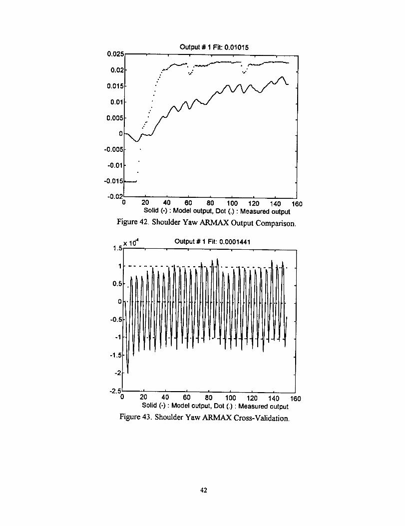
0.025
0.02
0.015
0.01
0.005
0
-0.005
-0.01
-0.015--..,
-0.02'0
Output # 1 Fit: 0.01015v = i v , | ,
• o l oe "°
I i I I I I I
20 40 60 80 100 120 140Solid (-) • Model output, Dot (.) • Measured output
Figure 42. Shoulder Yaw ARMAX Output Comparison.
xl01.5
Output # 1 Fit: 0.0001441
160
1
0.5
0
-2.50 20 40 60 80 100 120 140
Solid (-) • Model output, Dot (.) • Measured output
Figure 43. Shoulder Yaw ARMAX Cross-Validation.
160
42
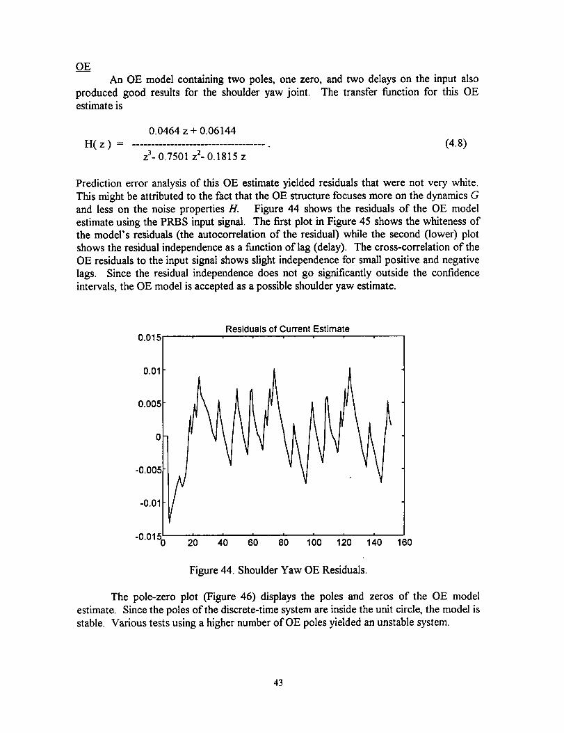
OE
An OE model containing two poles, one zero, and two delays on the input also
produced good results for the shoulder yaw joint. The transfer function for this OE
estimate is
0.0464 z + 0.06144
H(z) .................................... .z3- 0.7501 z2- 0.1815 z
(4.8)
Prediction error analysis of this OE estimate yielded residuals that were not very white.
This might be attributed to the fact that the OE structure focuses more on the dynamics G
and less on the noise properties H. Figure 44 shows the residuals of the OE model
estimate using the PRBS input signal. The first plot in Figure 45 shows the whiteness of
the model's residuals (the autocorrelation of the residual) while the second (lower) plot
shows the residual independence as a function of lag (delay). The cross-correlation of the
OE residuals to the input signal shows slight independence for small positive and negative
lags. Since the residual independence does not go significantly outside the confidence
intervals, the OE model is accepted as a possible shoulder yaw estimate.
0.005
-0.005
-0.01
-0.015 0
Residuals of Current Estimate
I I I I I I I
20 40 60 80 100 120 140 160
Figure 44. Shoulder Yaw OE Residuals.
The pole-zero plot (Figure 46) displays the poles and zeros of the OE model
estimate. Since the poles of the discrete-time system are inside the unit circle, the model is
stable. Various tests using a higher number of OE poles yielded an unstable system.
43

Correlation function of residuals. Output # 11
0.5
0
5; ' 1'0 ' '-0. 5 15 20 25lag
Cross corr. function between input 1 and residuals from out )ut0.4
0.20-0.2
%0 _o ....- -10 0 10 20 30lag
Figure 45. Shoulder Yaw OE Residual Whiteness and Independence.
2
1.5
1
0.5
............. 0
-0.5
-1
-1.5
OUTPUT # 1 INPUT # 1
-_ _ ; 2
Figure 46. Shoulder Yaw OE Pole-Zero Plot.
44
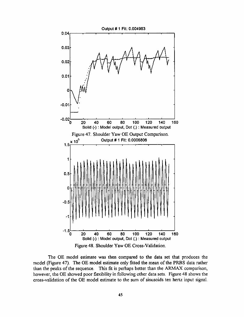
0.04Output # 1 Fit: 0.004963
0.03
0.02
0.01
-0.020 20 40 60 80 100 120 140 160
Solid (-) "Model output, Dot (.) • Measured output
Figure 47. Shoulder Yaw OE Output Comparison.
x 10a Output # 1 Fit: 0.00068061.5
0.5
0
-0.5
-1
-1.50 20 40 60 80 100 120 140 160
Solid (-) • Model output, Dot (.) • Measured output
Figure 48. Shoulder Yaw OE Cross-Validation.
The OE model estimate was then compared to the data set that produces the
model (Figure 47). The OE model estimate only fitted the mean of the PRBS data rather
than the peaks of the sequence. This fit is perhaps better than the ARMAX comparison,
however, the OE showed poor flexibility in following other data sets. Figure 48 shows the
cross-validation of the OE model estimate to the sum of sinusoids ten hertz input signal.
45
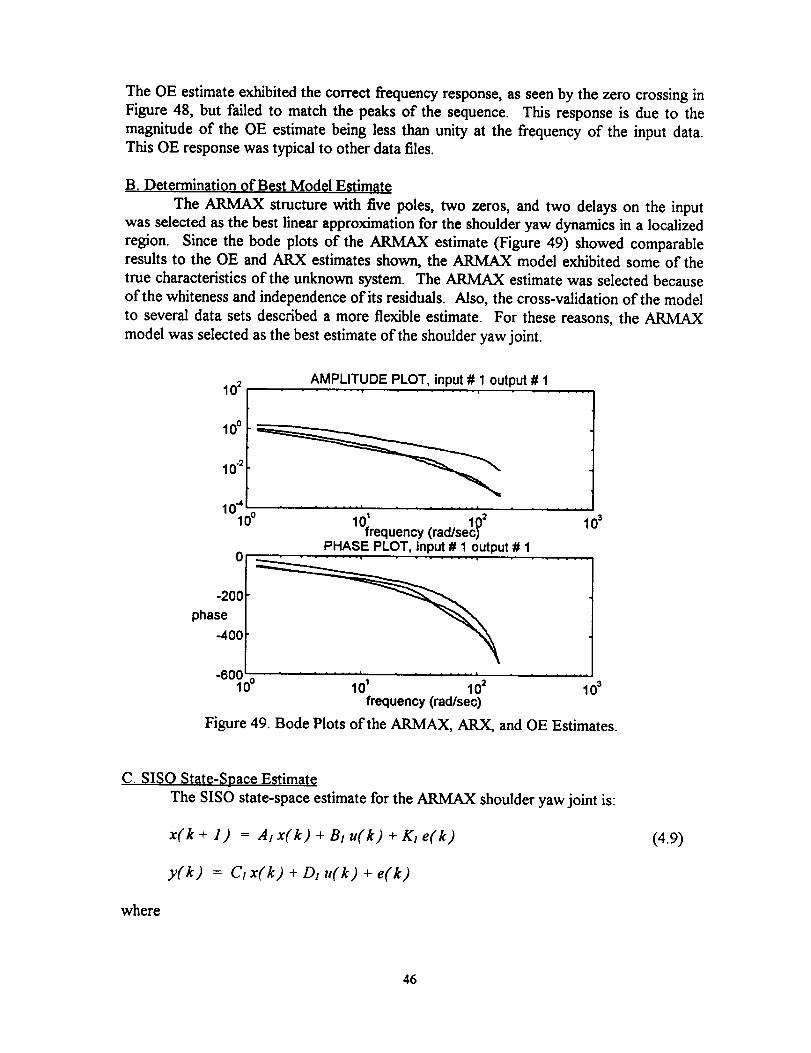
The OE estimate exhibited the correct frequency response, as seen by the zero crossing in
Figure 48, but failed to match the peaks of the sequence. This response is due to the
magnitude of the OE estimate being less than unity at the frequency of the input data.
This OE response was typical to other data files.
B. Determination of B¢s¢ Mode! Eetimate
The ARMAX structure with five poles, two zeros, and two delays on the input
was selected as the best linear approximation for the shoulder yaw dynamics in a localized
region. Since the bode plots of the ARMAX estimate (Figure 49) showed comparable
results to the OE and ARX estimates shown, the ARMAX model exhibited some of the
true characteristics of the unknown system. The ARMAX estimate was selected because
of the whiteness and independence of its residuals. Also, the cross-validation of the model
to several data sets described a more flexible estimate. For these reasons, the ARMAX
model was selected as the best estimate of the shoulder yaw joint.
102AMPLITUDE PLOT, input # 1 output # 1
...... i
,oo 10.2
1O;OO ......' 0;requency (radls;ii = 103
PHASE PLOT, input # 1 output # 1
-200
phase _
- oot- • .... i - --L
-6000° 101 102 103frequency (rad/sec)
Figure 49. Bode Plots of the ARMAX, AEX, and OE Estimates.
C. SISO State-Space Estimate
The SISO state-space estimate for the ARMAX shoulder yaw joint is:
x(k + 1) = As x(k) + Bt u(k) + KI e(k)
y(k) = Ct x(k) + Dj u(k) + e(k)
where
(4.9)
46
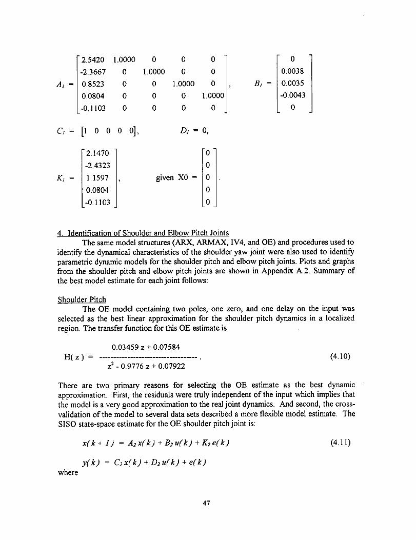
AI
2.5420
-2.3667
= 0.8523
0.0804
-0.1103
1.0000
0
0
0
0
0
1.0000
0
0
0
0
0
1.0000
0
0
0
0
0
1.0000
0
B1 =
0
0.0038
0.0035
-0.0043
0
C1 =
K1 =
[1 0 0
2.1470
-2.4323
1.1597
0.0804
-0.1103
0], 01 =
given X0 =
,
0
0
i0
!0
10
4. Identification of Shoulder and Elbow Pitch Joints
The same model structures (ARX, ARMAX, IV4, and OE) and procedures used to
identify the dynamical characteristics of the shoulder yaw joint were also used to identify
parametric dynamic models for the shoulder pitch and elbow pitch joints. Plots and graphs
from the shoulder pitch and elbow pitch joints are shown in Appendix A.2. Summary of
the best model estimate for each joint follows:
Shoulder Pitch
The OE model containing two poles, one zero, and one delay on the input was
selected as the best linear approximation for the shoulder pitch dynamics in a localized
region. The transfer function for this OE estimate is
0.03459 z + 0.07584
H( z ) .................................... . (4.10)z 2- 0.9776 z + 0.07922
There are two primary reasons for selecting the OE estimate as the best dynamic
approximation. First, the residuals were truly independent of the input which implies that
the model is a very good approximation to the real joint dynamics. And second, the cross-
validation of the model to several data sets described a more flexible model estimate. The
SISO state-space estimate for the OE shoulder pitch joint is:
x(k + l) = A2x(k) + B2u(k) + K2e(k) (4.11)
y(k) = C2 x(k) + D2 u(k) + e(k)where
47

0.9776A2 =
-0.0792
1.0000-
0, B2 =
c_--[1.ooooo1, D_--
[:I, ,vonxo:
0.0346]
0.0758-]
0,
[:1Elbow Pitch
An ARMAX model containing two poles, one zero, and two delays on the input
was found to sufficiently characterize the dynamics of the elbow pitch joint. The transferfunction for this model estimate is expressed as
0.01237 z + 0.0426
H(z) .......................................... .z3- 1.488 z2+ 0.5435 z
(4.12)
There are two primary reasons for selecting the ARMAX estimate as the best dynamic
approximation. First, the residuals were whiter than the OE estimate indicating that the
ARMAX appropriately modeled the noise characteristics of the joint. And second, the
cross-validation of the model to several data sets described a more flexible model estimate.
The SISO state-space estimate for the ARMAX elbow pitch joint is:
x(k + l) = A3x(k) + B3u(k) + K3e(k) (4.13)
y(k) = C_ x(k) + D3 u(k) + e(k)
where
1.4877
Aa = -0.5435
0
1.0000
0
0
c, = [1.0o0oo o],
1.4698 1
0
1.0000 ,
0
93 = 0,
given X0 =
B3 =
48

5. State-Space Multivariable Representation
Each SISO state-space estimate previously determined was identified about an
operating point. For the purpose of this identification, the operating point was chosen to
coincide with the insertion point trajectory vector for the RPCM ORU exchange task.
With each input signal producing only small deviations around the operating point, a local
neighborhood was defined about the RPCM insertion point for which each identified SISO
model is valid. This is the essence of linear approximation of a nonlinear model [18].
The following three-joint, linear, multivariable state-space estimate was formed
using each joint's best dynamic SISO representation:
x(k + l) = Ax(k) + Bu(k) + Ke(k) (4.14)
y(k) = Cx(k) + D u(k) + e(k)
where
A l 0 0 B I 0 0
A = A 2 0 , B = B 2 0 ,
0 A 3 0 B 3
j [00]C l 0 0 D I 0 0
C = C: 0 , D = D 2 0 ,
0 C 3 0 D 3
K
Ii I 0 0K 2 0
0 K 3
The matrices A,, B., C,, D,, and K. where n = 1, 2, or 3 refer to matrices previously
determined in equations 4.9, 4.11, and 4.13. This multivariable state-space estimate will
be used for comparison purposes. The actual RPCM data set along with several MIMOdata sets will be used to cross-validate this multivariable estimate.
49
V. Parametric Model Estimation:
Observer/Kalman Filter Identification
Among alternate system identification procedures are the ones based on system
realization theory. One such technique, used in the identification of space structures, is
Observer/Kalman Filter Identification (OKID). This technique computes Markov
parameters from pulse system response histories using an asymptotically stable observer to
form a stable discrete state-space model. This chapter will briefly discuss the OKID
technique provided in the System/Observer/Controller Identification Toolbox (SOCIT) by
Jer-Nan Juang, Lucas G• Horta, and Mirth Phan [19]. Residual analysis and cross-
validation procedures will be used to identify the best state-space models for the HMTBjoints•
1. OKID Background and Procedure
When a pulse sequence is used as input into the discrete-time state-space dynamicequation
x(k + 1) = A x(k) + B u(k) (5.1)
y(k) = C x(k) + D u(k),
the resulting series of equations can be formed into a pulse-response matrix Y, that is,
V = [ D CB CAB ..... C AkIB ]. (5.2)
The elements of the matrix Y are known as the system Markov parameters. System
realization involves determining the matrices A, B, C, and D from the system Markov
parameters to satisfy the state and measurement equations (5.1) [8]. Minimum realization
theory, attributed to Ho and Kalman [12], determines a model with the smallest state-
space dimension among all realizable systems. The procedure starts by forming the
generalized Hankel matrix composed of Markov parameters in the following manner:
H(k-1) =
Yk+l Yk+2 .. Yk÷_ J .
(5.3)
If the number of rows a and the number of columns fl are greater than the order of the
system, then the Hankel matrix is of rank n. This realization algorithm extracts linear
state-space matrix components from noise-free data.
For noisy input/output sequences, the Eigensystem Realization Algorithm (ERA)
produces better results [8]. By deleting specific rows and columns of the Hankel matrix,
ERA forms a block data matrix composed of strongly measured Markov sequence
components. A minimum realization may be obtained by factorization of the block data
50
matrix using singular value decomposition. The order of the identified system is
determined by selecting the number of significant singular values.
Observer/Kalman Filter Identification is determined by inserting an observer into
the discrete-time state-space dynamic equation (5.1) to form the discrete-time state-space
observer model
x(k + l) = A x(k) + B v(k) (5.4)
y(k) = Cx(k) + D u(k),
where
A = A+GC,
D
B = [ B+GD -G], and
v(k)= Iu(k) 1.
Ly(k)_J
When a pulse sequence is used as input into the observer model (5.4), the following
observer Markov parameters may be computed:
= [D CB CAB ..... C'_k"_ l. (5.5)
The OKID technique then computes the system Markov parameters from the observer
Markov parameters for minimum realization of a state-space model estimate. It is obvious
from (5.5) that the matrices A, B, C, and D are embedded in the observer Markov
parameters. Since the observer gain G may be arbitrarily chosen, the OKID routine
creates a deadbeat observer by simply placing all the eigenvalues of A at the origin
producing an asymptotically stable observer. Setting G to be the deadbeat observer gain
allows for a minimum number of Markov parameters to describe the input/output
relationship of a system [8].
Juang [8] describes the relationship between the state-space observer model and
the Kalman filter equation
X(k+ l) = AX(k)+Bu(k)+K_r(k) (5.6)
where
(k}
¢¢(k}K
= c (k} + Du(k),
is the estimated state,
is the estimated measurement,
is the Kalman filter gain, and
51
ocr (k) is the residual defined as the difference y(k) -y (k).
The observer gain is said to be the steady-state Kalman filter gain
g=-a (5.7)
in theory if the residuals are identically zero, C r (k) = 0, and the data length is
sufficiently long to produce negligible truncation error. Theoretical background of the
OKID technique is found in the text Applied System Identification by Jer-Nan Juang [8].
For each joint, system and observer parameters will first be determined. Next, theassociated prediction errors will be computed. The Hankel matrix will be shown for
proper order selection. After selecting the system order from the Hankel singular values,
the state-space estimate will be realized. This realization will also yield the Kalman filter
gain which for the purposes of this investigation will be approximated to the observer gain
since each estimate will be selected to minimize the residuals and the arm will be operatedin a localized region to minimize system nonlinearities. Each model estimate will be
compared to the data set that produced the model as well as cross-validated to another
data set. A three-joint multivariable state-space model will be determined from the threeSISO state-space estimates.
2. Identification of Shoulder Yaw Joint
A. Determine Markov Parameter Set
An upper bound for the OKID model order must first be specified to compute an
estimate. Using a fifth order system as the upper bound, five independent observer
parameters were initially computed to identify the shoulder yaw state-space model using
the PRBS input/output data. The system and observer Markov parameters for the
shoulder yaw joint are shown in Figure 50. As seen in Figure 50, the rate of decay for the
observer parameters is much larger than that for the system Markov parameters. This
demonstrates the advantage of the deadbeat observer in minimizing the number of pulse
response samples used to realize the state-space equation [8]. The relatively high number
of independent Markov parameters shown in the plot indicates that the shoulder yaw jointexhibits relatively significant nonlinear characteristics.
52
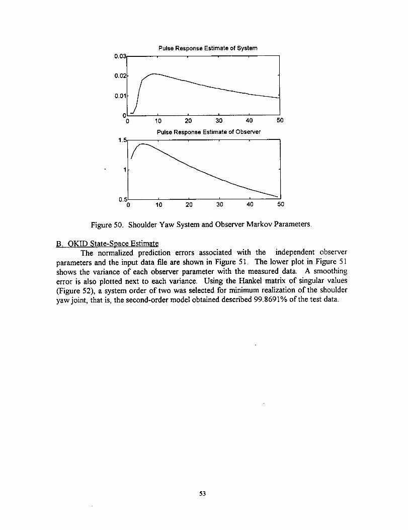
0.03
0.02
0.01
00
1.5
Pulse Response Estimate of Systemv
i I i
10 20 30 40
Pulse Response Estimate of Observer
50
0.50 10 20 30 40 50
Figure 50. Shoulder Yaw System and Observer Markov Parameters.
B. OKID State-Space Estimate
The normalized prediction errors associated with the independent observer
parameters and the input data file are shown in Figure 51. The lower plot in Figure 51
shows the variance of each observer parameter with the measured data. A smoothing
error is also plotted next to each variance. Using the Hankel matrix of singular values
(Figure 52), a system order of two was selected for minimum realization of the shoulder
yaw joint, that is, the second-order model obtained described 99.8691% of the test data.
53
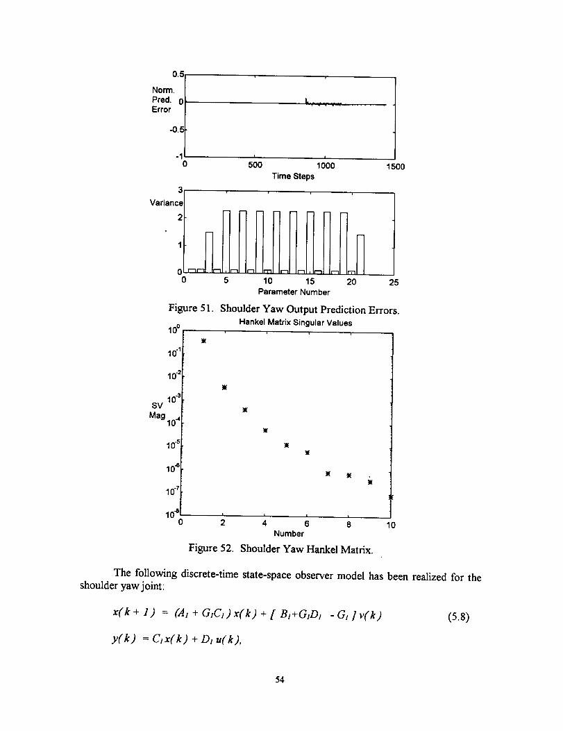
0.5
Norm.
Pred. 0Error
-0..=
-10
3
Variance
2
1
00
lO0
10-1
L ............
I I
500 1000 1500
Time Steps
5 10 15 20 25Parameter Number
Figure 51. Shoulder Yaw Output Prediction Errors.
Hankel Matrix Singular Values= i
lO+SV
Mag 10"4
lff s
lO•
10-7
100
]K
2 4 6 8Number
Figure 52. Shoulder Yaw Hankel Matrix.
10
The following discrete-time state-space observer model has been realized for theshoulder yaw joint:
x(k + 1) = (AI + GICI) x(k) + [ B1+GIDI - Gt ] v(k) (5.8)
y(k) = Clx(k) + DI u(k),
54
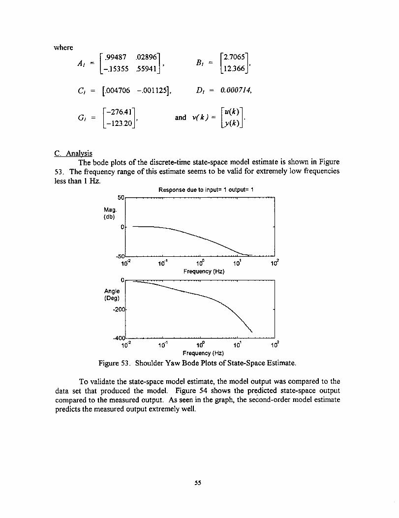
where
__r.9948,.0=8961A, L-.15355 55941J' B, = L12.366j,
C, = [.004706 -.001125], D, = 0.000714,
r.<,,,lG, = -123.20J' and v(k)= Iy(k)- 1.
C. Analysis
The bode plots of the discrete-time state-space model estimate is shown in Figure
53. The frequency range of this estimate seems to be valid for extremely low frequencies
less than 1 Hz.
Response due to input= 1 output= 150 ........
Mag.(db)
-50 , ' .......10.2 10-1 100 101
Frequency (Hz)
0
Angle,Oe_ ;Ot-400' ........................
10-2 10"1 10° 101
Frequency (Hz)
Figure 53. Shoulder Yaw Bode Plots of State-Space Estimate.
To validate the state-space model estimate, the model output was compared to the
data set that produced the model. Figure 54 shows the predicted state-space output
compared to the measured output. As seen in the graph, the second-order model estimate
predicts the measured output extremely well.
55
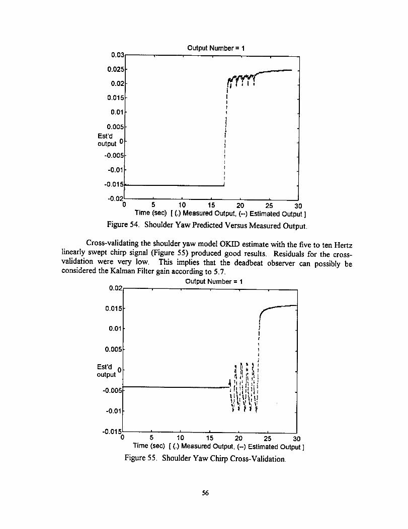
0.03
0.025
0.02
0.015
0.01
0.005
Est'doutput 0
-0.00. t
-0.01
-0.01,=
-0.020
Figure 54.
Output Number = 1
I I I I I
5 10 15 20 25 30
Time (sec) [ (.) Measured Output, (-) Estimated Output ]
Shoulder Yaw Predicted Versus Measured Output.
Cross-validating the shoulder yaw model OKID estimate with the five to ten Hertz
linearly swept chirp signal (Figure 55) produced good results. Residuals for the cross-
validation were very low. This implies that the deadbeat
considered the Kalman Filter gain according to 5.7.
Output Number = 10.02
0.015
0.01
0.005
Est'd 0output
-0.005
-0.01
-0.0150
observer can possibly be
r------
Figure 55.
• _: I j I:._1 $.(:l!l,IJ
I I I I I
5 10 15 20 25 30Time (sec) [ (.) Measured Output, (-) Estimated Output ]
Shoulder Yaw Chirp Cross-Validation.
56
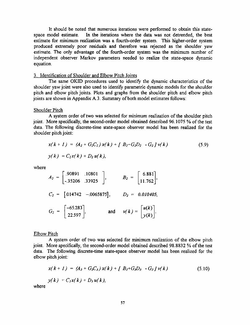
It should be noted that numerous iterations were performed to obtain this state-
space model estimate. In the iterations where the data was not detrended, the best
estimate for minimum realization was a fourth-order system. This higher-order system
produced extremely poor residuals and therefore was rejected as the shoulder yaw
estimate. The only advantage of the fourth-order system was the minimum number of
independent observer Markov parameters needed to realize the state-space dynamic
equation.
3. Identification of Shoulder and Elbow Pitch Joints
The same OKID procedures used to identify the dynamic characteristics of the
shoulder yaw joint were also used to identify parametric dynamic models for the shoulder
pitch and elbow pitch joints. Plots and graphs from the shoulder pitch and elbow pitch
joints are shown in Appendix A.3. Summary of both model estimates follows:
Shoulder Pitch
A system order of two was selected for minimum realization of the shoulder pitch
joint. More specifically, the second-order model obtained described 96.1075 % of the test
data. The following discrete-time state-space observer model has been realized for the
shoulder pitch joint:
x(k + 1) = (A_ + G2C_)x(k) + [ B_+G_D2 -G_lv(k) (5.9)
y(k) = C2x(k) + u(k),
where
= [.90891 .I0801 ] B2= [ 688'IA_ L-.35206 .33925 ' L11.762J'
c2 = [.014742 -.0065875], /92 = 0.010405,
62 = and v(k) = ["(k)l.Ly(k)J
Elbow Pitch
A system order of two was selected for minimum realization of the elbow pitch
joint. More specifically, the second-order model obtained described 98.8832 % of the test
data. The following discrete-time state-space observer model has been realized for the
elbow pitch joint:
x(k + 1) = (A.3 + G3C._)x(k) + [ B3+G.,_D3 -G3]v(k) (5.10)
y(k) = C3x(k) + D3 u(k),
where
57
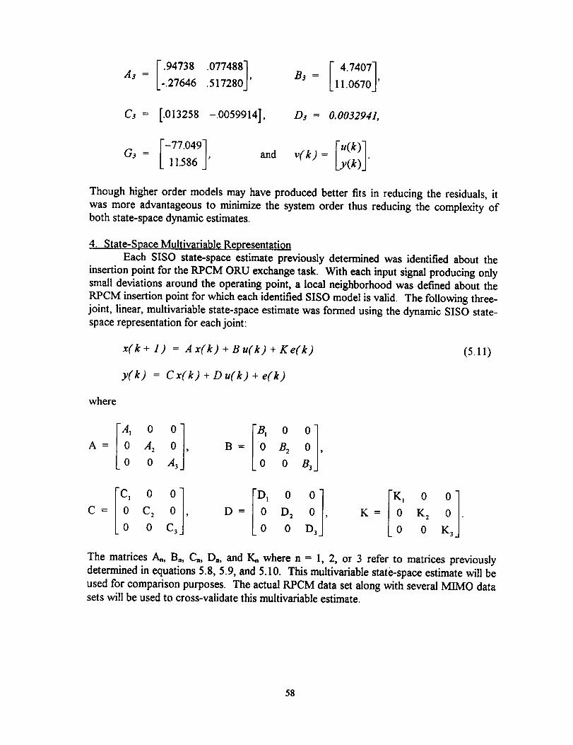
= .o 4,sI lA_ I_-.27646 .517280J' B_ = I 1.0670I'
C3 = [.013258 -.0059914], D_ = 0.0032941,
F-77.o491 F,(k)].G_ = L 11.586 .]' and v(k) = LY(k)J
Though higher order models may have produced better fits in reducing the residuals, it
was more advantageous to minimize the system order thus reducing the complexity ofboth state-space dynamic estimates.
4. State-Space Multivariable Representation
Each SISO state-space estimate previously determined was identified about the
insertion point for the RPCM ORU exchange task. With each input signal producing onlysmall deviations around the operating point, a local neighborhood was defined about the
RPCM insertion point for which each identified SISO model is valid. The following three-
joint, linear, multivariable state-space estimate was formed using the dynamic SISO state-space representation for each joint:
x(k + l) = Ax(k) + Bu(k) + Ke(k) (5.11)
y(k) = Cx(k) + D u(k) + e(k)
where
i!,0o] o0A = A 2 0 , B = B 2 0
0 A3 0 B3
i!00] ii001 i!0ojC = C 2 0 , D = D 2 0 , K = K 2 0 .
0 C 3 0 D 3 0 K 3
The matrices A,, B,, C,, D,, and K_ where n = 1, 2, or 3 refer to matrices previously
determined in equations 5.8, 5.9, and 5.10. This multivariable state-space estimate will be
used for comparison purposes. The actual RPCM data set along with several MIMO data
sets will be used to cross-validate this multivariable estimate.
58
VI. Comparison of Identified Models
This chapter will compare the multivariable state-space model estimate obtained
using prediction error techniques within Lennart Ljung's System Identification Toolbox
and the multivariable state-space model estimate obtained using the Observer/Kalman
Filter identification (OKID) technique provided in the System�Observer/Controller
Identification Toolbox (SOCIT) by Jer-Nan Juang, Lucas G. Horta, and Minh Phan.
Frequency plots and pole/zero maps for each estimate will be shown. Both multivariable
estimates will be compared to data sets obtained from an RPCM experiment and a MIMO
experiment using the chirp signal. Fit comparisons and residual analysis will be performed
for each state-space estimate.
1. Identified Model Forms
The identification techniques investigated and described in the previous chapters
represent parametric models of the form
y(t) = G(q) u(t) + v(t) (6.1)
where
G(q) is the open-loop transfer function, and
v(t) represents the disturbances.
This linear equation attempts to describe the open-loop dynamic characteristics of each of
the three HMTB joints with additive disturbances. It should be noted that this dynamic
equation is, in essence, an open-loop representation of the actual closed-loop dynamical
implementation for each joint. This implies that the actual closed-loop dynamics will be
embedded within the open-loop description of each joint. For high noise-to-signal ratios in
the I/O time histories of each joint, the disturbances may be represented as
v(t) : H(q) e(t) (6.2)
where
H(q) is the disturbance dynamics, and
e(t) represents white noise.
In the System Identification Toolbox, prediction error techniques were used to
determine ARMAX and OE black-box model structures for each joint. The ARMAX
structure forms the joint dynamics according to the block diagram shown in Figure 56.
The OE structure differs from the ARMAX structure by allowing the disturbances (noise)
to go unfiltered as shown in Figure 57. The parametric black-box model developed for
each joint was then converted to a SISO state-space estimate.
59
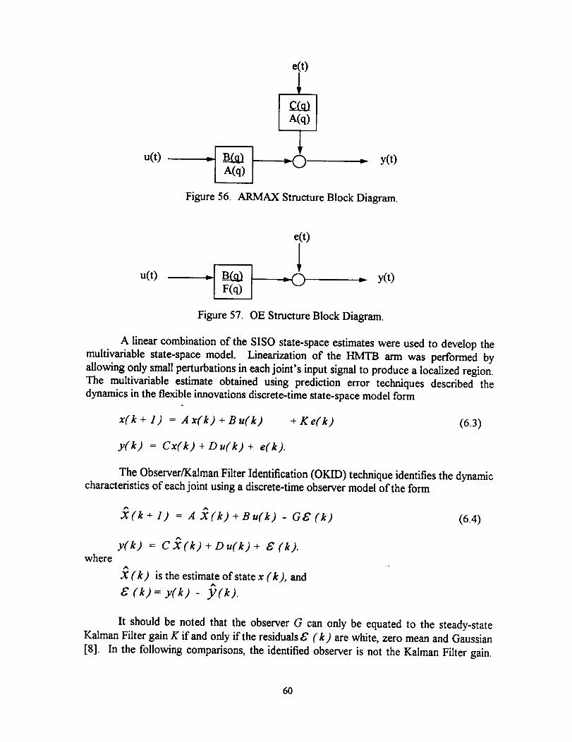
e(t)
u(t) =1 I
i A(q)i = y(t)I |
Figure 56. ARMAX Structure Block Diagram.
e(t)
u(t) -I B_cq I-I F(q)[ =O -_ y(t)
Figure 57. OE Structure Block Diagram.
A linear combination of the SISO state-space estimates were used to develop the
multivariable state-space model. Linearization of the HMTB arm was performed by
allowing only small perturbations in each joint's input signal to produce a localized region.
The multivariable estimate obtained using prediction error techniques described the
dynamics in the flexible innovations discrete-time state-space model form
x(k + 1) = A x(k) + B u(k) + Ke(k) (6.3)
y(k) = Cx(k) + D u(k) + e(k).
The Observer/Kalman Filter Identification (OKID) technique identifies the dynamiccharacteristics of each joint using a discrete-time observer model of the form
._(k + 1) = A ._(k) + Bu(k) - Gg (k) (6.4)
wherey(k) = C X(k) + Du(k) + oc (k).
(k) is the estimate of state x (k), and
c (k)= y(k) - f_(k).
It should be noted that the observer G can only be equated to the steady-state
Kalman Filter gain K if and only if the residuals g' (k) are white, zero mean and Gaussian
[8]. In the following comparisons, the identified observer is not the Kalman Filter gain.
60

The computedobserverG simply minimizes the residuals due to nonlinearities in each
joint, non-whiteness of the noise processes, and correlation effects between the residual
and the input signal.
Both multivariable model estimates will be compared using equivalent state-space
representations, that is K = -G where K in this case is simply a residual filter. For
notation purposes, the multivariable model identified using prediction error techniques will
be called the SysID model and the model identified using the Observer/Kalman Filter
Identification (OKID) technique will be called the OKID model.
2. Transfer Function Analysis
The transfer function G(q) from equation 6.1 may expressed in terms of the state-
space matrices A, B, C, and D as
G( q ) = C ( q I - A )I B + D. (6.5)
Bode plots for the SysID MIMO model shown in Figures 58 - 60 describe the frequency
and phase response characteristics of the shoulder yaw, shoulder pitch, and elbow pitch
joints, respectively.
0
Gain dB
-50
0
- 180Phase
(deg)-36C
-54C
10.2 10 "1
Figure 58.
0 ..... ;;;i ; ; ;;;;;;i ; ; ; ;;;;;i ; ; ;E;;;;I ........
.... .---.-.,- : 1 :st.-----:-- "-i _ _ .... ---t-- _-;--:-;-:-:-:l .... "--:--:- t-.'-:-:f: ..... :-- -:-.7-." {'i"
....iiiiiiiiiiiii ii iiiiiiilo -_ aoo lO_ lo2 lO3
Frequency (rad/sec)input 1
i i i ii i il iiiiiiii i_ il i il ili ! !ii.... ... e..,. t = H t......,.. I. _ .,.l_,_ .... 1. ° t ._ _.....,..1 .... _. ... k _ .._l,.....,...'..,. _ J _ _t
lo ° lo 1 lo _ lo3Frequency (rad/sec)
Sys[D Shoulder Yaw Bode Plots.
61
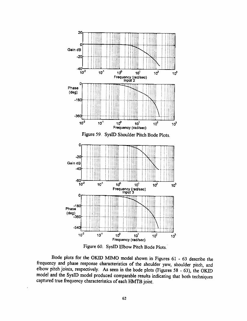
i iiii_ii!i iiiiiiiii!iii!iiii iiiiiiiii iiiiiii
o.......iiiiiiiL_iii_i!__ii_ii_Gain dB
-20
( J I I I
"4_0-2 10-1 10o 101 102 103
Frequency. _ad/sec)mpu(_
0
-i i ii;ii;l-,, iJJlJ!;j!J!iEijiiEEii!iif!iii!!iJ!j!ijii-18( ..............
. ....iJJiiiiiiif!10.2 10-1 100 101 102 103
Frequency (rad/sec)
Figure 59. SysID Shoulder Pitch Bode Plots.
-20
Gain dB
-40
0
-180Phase
(deg_)360
-541
....iiii!!!iiiii.... ii!i!ii..............i!ii!........."602 10"I 100 101 102 103
Frequency. _ad/sec)inpu(_
i!!iii!iiiii!!iiiiiiii !iljji!iili ii11111; i ii_;i;_i : ::::::i i ii_iiil; i"i_iiiil
1#10"2 10"1 10o 101 102
Frequency (rad/sec)
Figure 60. SysID Elbow Pitch Bode Plots.
Bode plots for the OKID MIMO model shown in Figures 6] - 63 describe the
frequency and phase response characteristics of the shoulder yaw, shoulder pitch, and
elbow pitch joints, respectively. As seen in the bode plots (Figures 58 - 63), the OKID
model and the SysID model produced comparable results indicating that both techniques
captured true frequency characteristics of each HMTB joint.
62
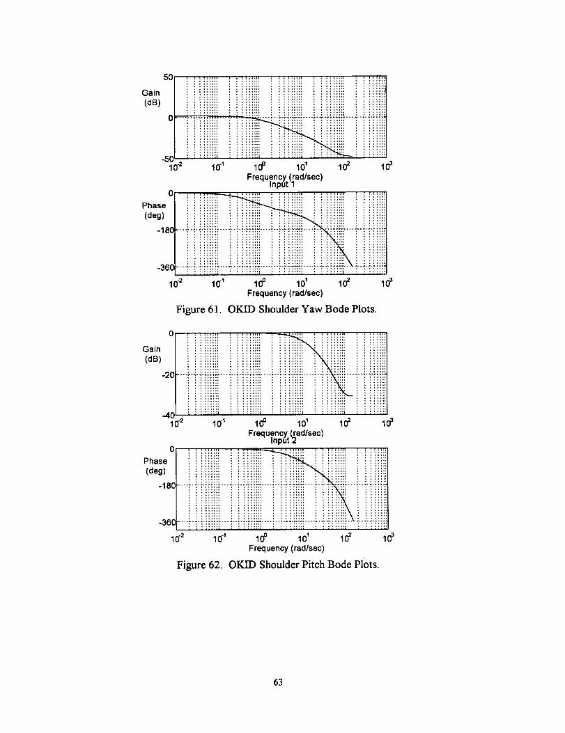
50 ; ; ; ;_;;_1 i i il;l_l i ; i ;;_Jll _ i ;;;;;_1 ; ; ;;;i;;:
! !_!!i!ii i _i!!!iii i iiiiiiii !!!!!!iii i i!iiiiiGain _ ii!!!_ii i iiii[!!i ! i!iiiiii i iiiiiii! i !!!i!!i
(dB) ::ii::i'::::::::::::::::::::::::::::::::: !i::iiii::i i ::iiii::i: : ::::::: : : ::::::: : :::::::: : : ::::::: : : ::::::
° 'i"i'i' iiii -5_'o2 lO" lO0 lO' lO2 o_
Frequency (radlsec)input 1
, , ..... - ; ;_;;;tl ; ; _;i;;;i .... ;;;;; ........
-360 ............................................
10.2 10"1 100 101 102 103Frequency (rad/sec)
OKE) Shoulder Yaw Bode ])lots.Figure 61.
0
Gain
(dB)
-20
0
Phase
(deg)
-18(:
Figure 62.
....i.i.i.ililil...i..t.i.iiiii.. i..i.l.iiiii_4_,o.2n lO" lO0 lO' lO= lO3
Frequency. (.[ad/sec)Input2
100 10' 102 103
Frequency (rad/sec)
OKE) Shoulder ])itch Bode ])lots.
63
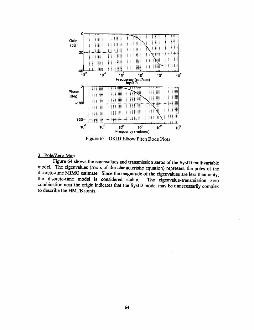
0
iiiiiiiiiiiiiiilliiiiiill!ii!!iiiii!iiiiii-20 ...................................
-4002 1_' lO0 lo 1 102 103
Frequency. _ad/sec)Input_
0
Phase(deg) iiiiiiiii! } iiiiiii iiiiiiifii__....i ii!iiiii! ! i!iiiiiiiill
-18C ...................................
....iiiiiiiiiij iJ10.2 10-1 10o 101 102 103
Frequency (racl/sec)
Figure 63. OKID Elbow Pitch Bode Plots.
3. Pole/Zero Map
Figure 64 shows the eigenvalues and transmission zeros of the SysID multivariable
model. The eigenvalues (roots of the characteristic equation) represent the poles of the
discrete-time MIMO estimate. Since the magnitude of the eigenvalues are less than unity,
the discrete-time model is considered stable. The eigenvalue-transmission zero
combination near the origin indicates that the SyslD model may be unnecessarily complexto describe the HMTB joints.
64
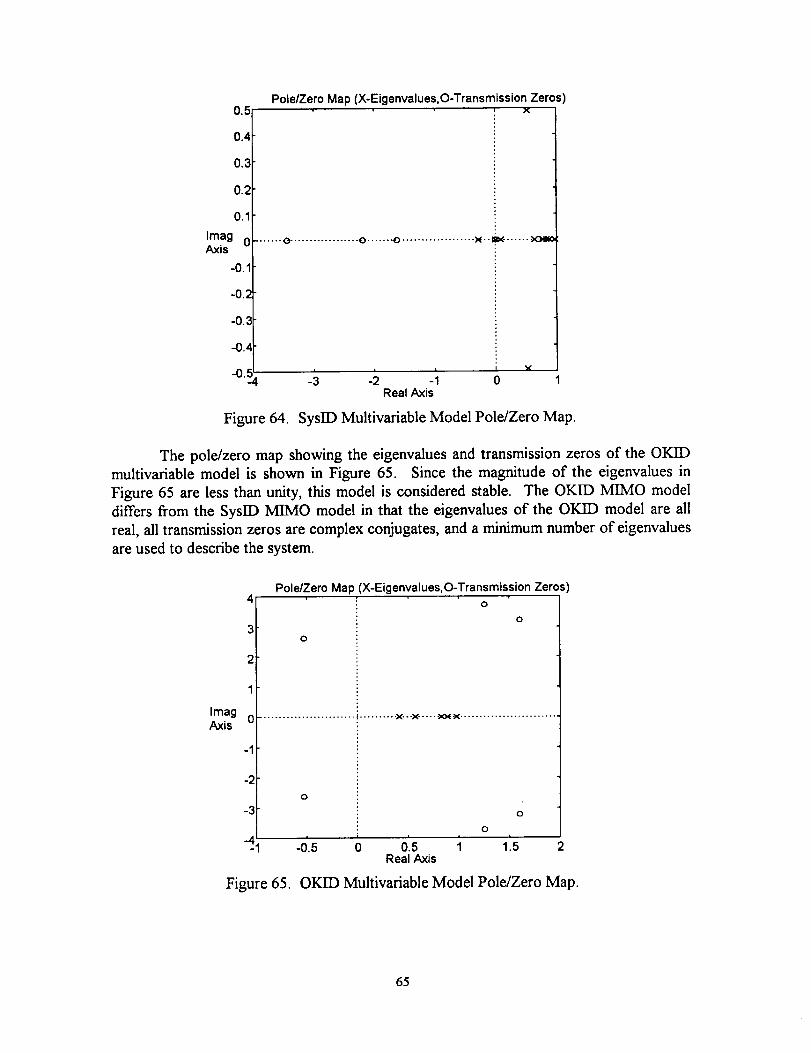
0.5
0.4
0.3
0.2
0.1
Imag 0Axis
-0.1
-0.2
-0._
-0.4
-0.5..Z
Figure 64.
Pole/Zero Map (X-Eigenvalues,O-Transmission Zeros)x
...... O .................. O ....... O ................... _--II1_ ......
vi i i
-3 -2 -1 0 1Real Axis
SysID Multivariable Model Pole/Zero Map.
The pole/zero map showing the eigenvalues and transmission zeros of the OKID
multivariable model is shown in Figure 65. Since the magnitude of the eigenvalues in
Figure 65 are less than unity, this model is considered stable. The OKID MIMO model
differs from the SyslD MIMO model in that the eigenvalues of the OKID model are all
real, all transmission zeros are complex conjugates, and a minimum number of eigenvalues
are used to describe the system.
ImagAxis
4
3
2
1
0
Pole/Zero Map (X-Eigenvalues,O-Transmission Zeros)O
O
-1
-2
-3
4_.
0
......................... i .......... X---X ..... .I,0,( _<........................
0
0
i i i i i
-0.5 0 0.5 1 1.5Real Axis
Figure 65. OKID Multivariable Model Pole/Zero Map.
65
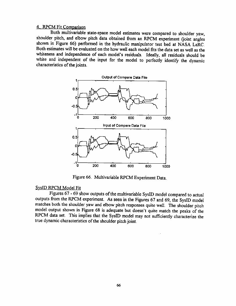
4. RPCM Fit Comparison
Both multivariable state-space model estimates were compared to shoulder yaw,
shoulder pitch, and elbow pitch data obtained from an RPCM experiment (joint angles
shown in Figure 66) performed in the hydraulic manipulator test bed at NASA LaRC.
Both estimates will be evaluated on the how well each model fits the data set as well as the
whiteness and independence of each model's residuals. Ideally, all residuals should be
white and independent of the input for the model to perfectly identify the dynamiccharacteristics of the joints.
Output of Compare Data File
0.5
0
-0._
0 200 400 600I
800 1000
Input of Compare Data File
0.5
0
-0.5
-10I I I I
200 400 600 800 1000
Figure 66. Multivariable RPCM Experiment Data.
SyslD RPCM Model Fit
Figures 67 - 69 show outputs of the multivariable SyslD model compared to actual
outputs from the RPCM experiment. As seen in the Figures 67 and 69, the SysID model
matches both the shoulder yaw and elbow pitch responses quite well. The shoulder pitch
model output shown in Figure 68 is adequate but doesn't quite match the peaks of the
RPCM data set. This implies that the SyslD model may not sufficiently characterize the
true dynamic characteristics of the shoulder pitch joint.
66
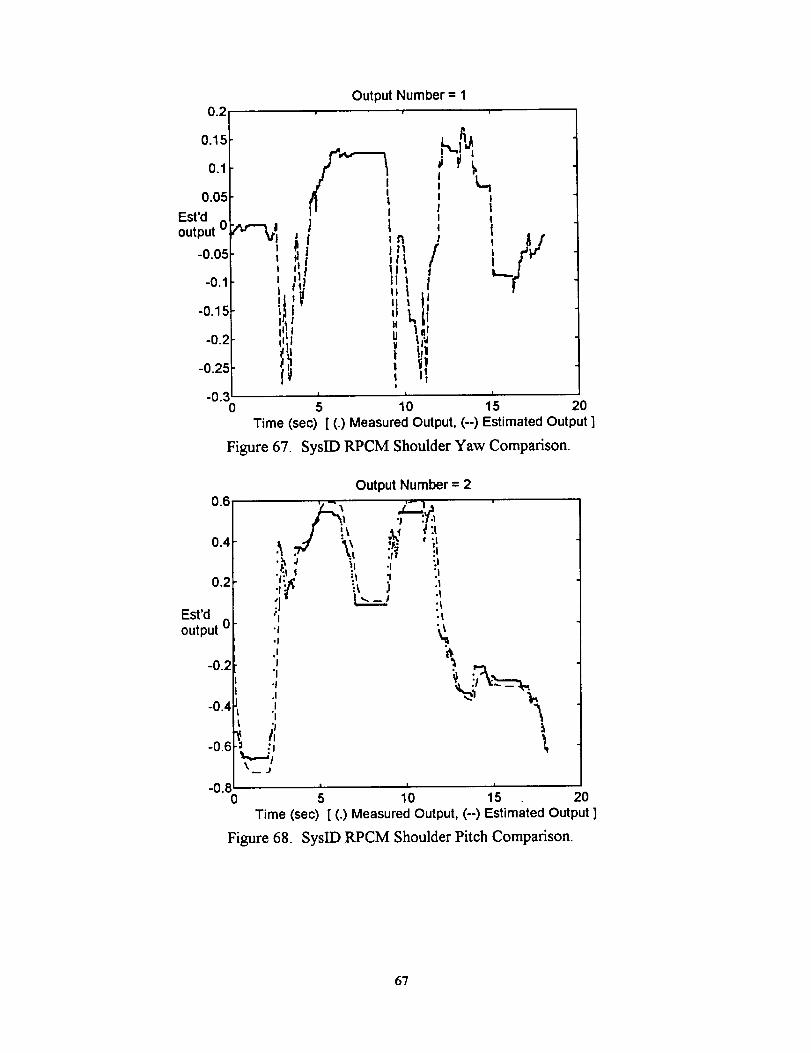
0.2
0.15
0.1
0.05
Est'd0
output
-0.05
-0.1
-0.15
-0.2
-0.25
-0.3
_j
:VI-!t
Output Number = 1=
, ¼I I
I I II !
I ,I ,, _I_j
I r , V
I I
0 5 15 20
f_11/iII111taII t
l!
u
!t!
I
10
Time (sec) [ (.) Measured Output, (--) Estimated Output ]
Figure 67. SysID RPCM Shoulder Yaw Comparison.
0.6
0.4
0.2
Est'doutput 0
-0.2
-0.4
-0.6
Output Number = 2
• h J
• _l t
"1,I
.I!
"1.!.II
"1
il
222
t ;I• I r :1
}1 -I "1
"1.|.t
.t
-0.8 ' ' '0 5 10 15 20
Figure 68.
Time (sec) [ (.) Measured Output, (--) Estimated Output ]
SyslD RPCM Shoulder Pitch Comparison.
67
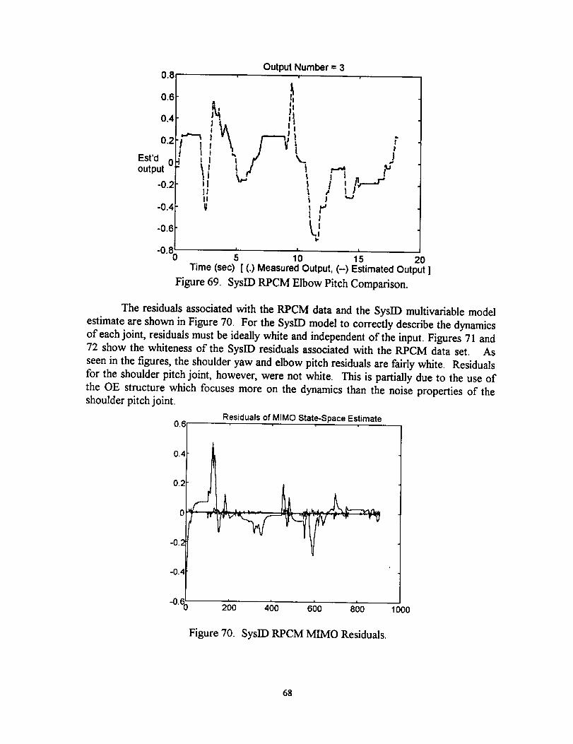
Output Number = 30.8
0.6
0.4
0.2
Est'd 0output
-0.2
-0.4
-0.6
-0.80
A
I'I
I I
!Jt!
i
%. !
l I |I )I[If
1'0 1_5 20Time (sec) [ (.) Measured Output, (-) Estimated Output ]
Figure 69. SysID RPCM Elbow Pitch Comparison.
The residuals associated with the RPCM data and the SysID multivariable model
estimate are shown in Figure 70. For the SysID model to correctly describe the dynamics
of each joint, residuals must be ideally white and independent of the input. Figures 71 and72 show the whiteness of the SysID residuals associated with the RPCM data set. As
seen in the figures, the shoulder yaw and elbow pitch residuals are fairly white. Residuals
for the shoulder pitch joint, however, were not white. This is partially due to the use of
the OE structure which focuses more on the dynamics than the noise properties of theshoulder pitch joint.
Residualsof MIMO State-Space Estimate0.6 ....
0.4
0.2
0
-0.
O_ 200 400 600 800 1000
Figure 70. SysID RPCM MIMO Residuals.
68
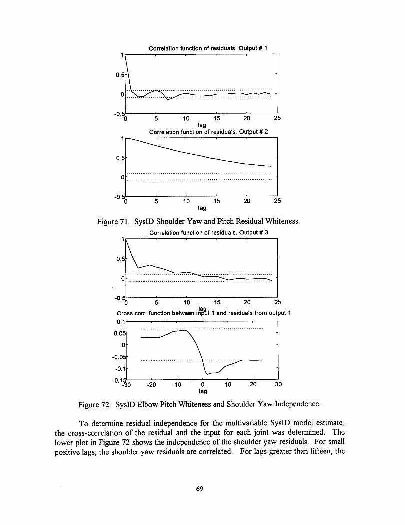
0
-0.5
0.5
-o.so
Figure 72.
Correlation function of residuals. Output # 1
Figure 71.
I I I I
0 5 10 15 20lag
Correlation function of residuals. Output # 2
25
i I I I
5 10 15 20 25
lag
SysID Shoulder Yaw and Pitch Residual Whiteness.
Correlation function of residuals. Output # 31
0.50'
-0.5 I I I I
5 10 15 20 25
0.1
0.0_=
0
-0.05
-0.1
-0.1_0
aCross corr. function between np'tJt1 and residuals from output 1
.........................................................
I I l I l
-20 -10 0 10 20 30lag
SysID Elbow Pitch Whiteness and Shoulder Yaw Independence.
To determine residual independence for the multivariable SysID model estimate,
the cross-correlation of the residual and the input for each joint was determined. The
lower plot in Figure 72 shows the independence of the shoulder yaw residuals. For small
positive lags, the shoulder yaw residuals are correlated. For lags greater than fifteen, the
69
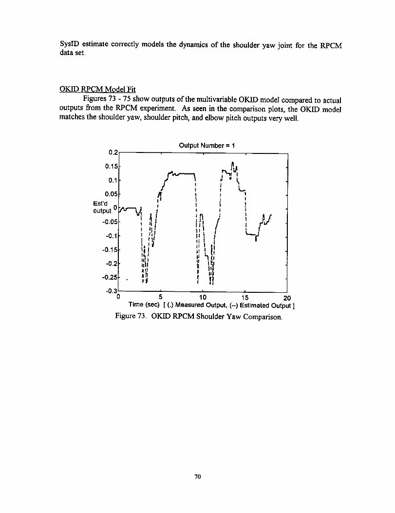
SysID estimate correctly models the dynamics of the shoulder yaw joint for the RPCMdata set.
OKID RPCM Model Fit
Figures 73 - 75 show outputs of the multivariable OKID model compared to actual
outputs from the RPCM experiment. As seen in the comparison plots, the OKID model
matches the shoulder yaw, shoulder pitch, and elbow pitch outputs very well.
0.2
0.15
0.1
0.05
Est'd
-0.05
-0.1
!iJlh!
-0.2 Idl
roll
-0.25 _11
-0.30
Figure 73.
Output Number = 1
I/1
I !t
11 a
11 3
II!!f1
I
J!!
JII
J
[
L.1!|i
11
I I I
5 10 15 20Time (sec) [ (.) Measured Output, (--) Estimated Output ]
OKID RPCM Shoulder Yaw Comparison.
70
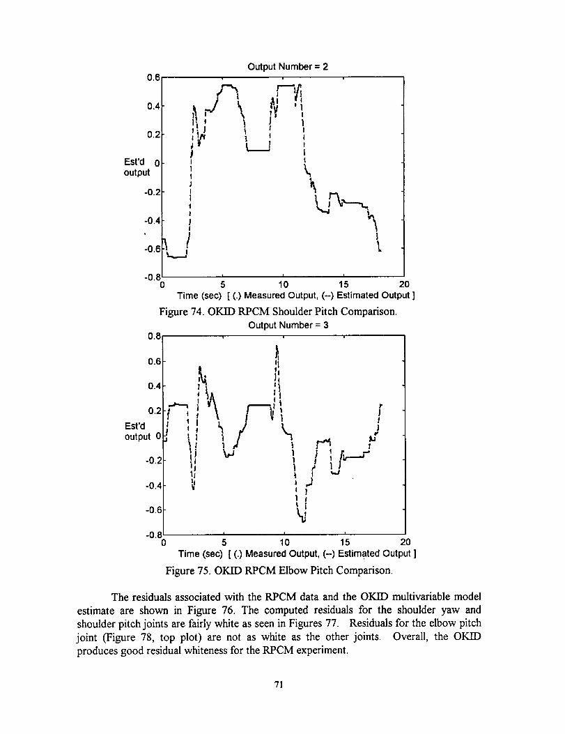
0.6
0.4
0.2
Est'd 0output
-0.2
1I
-0.4 !I
Output Number = 2
I 1
I tI||
1II
0"6I_!
_0.8/0 5
I
k
I
I I
10 15 20Time (sec) [ (.) Measured Output, (-) Estimated Output ]
Figure 74. OKID RPCM Shoulder Pitch Comparison.
Output Number = 30.8 , , ,
0.6
0.4
0.2
Est'doutput 0
-0.2
-0.4
-0.6
-0.8 I0
!
t I
Ij11!fI
I!1
l
1')!
t
| i
I
10I I
5 15 20Time (sec) [ (.) Measured Output, (--) Estimated Output ]
Figure 75. OIGD RPCM Elbow Pitch Comparison.
The residuals associated with the RPCM data and the OKID multivariable model
estimate are shown in Figure 76. The computed residuals for the shoulder yaw and
shoulder pitch joints are fairly white as seen in Figures 77. Residuals for the elbow pitch
joint (Figure 78, top plot) are not as white as the other joints. Overall, the OKID
produces good residual whiteness for the RPCM experiment.
71
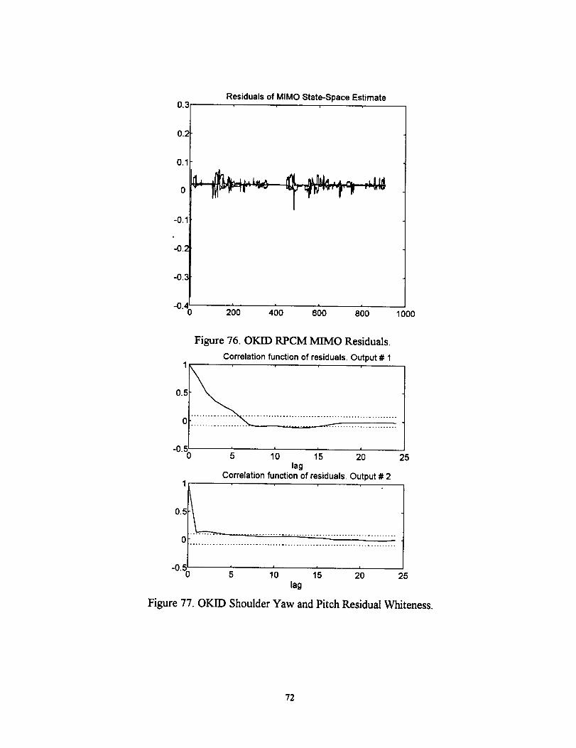
0.3
0.2
0.1
0
-0.1
-0.2
-0.3
Residuals of MIMO State-Space Estimate
0 0 | i i-0. 2 0 400 600 800 1000
0.5
0
-0._=
Figure 76. OKID RPCM MIMO Residuals.
Correlation function of residuals. Output # 1
...........i iiiiiiiio
I | I I
0 5 10 15 20 25lag
Correlation function of residuals. Output # 21
0.5
0........................................................................
fi I I I I
"0'-0 5 10 15 20 25
lag
Figure 77. OKID Shoulder Yaw and Pitch Residual Whiteness.
72
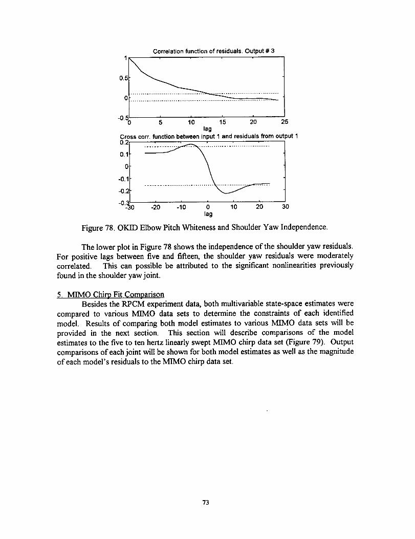
Correlation function of residuals. Output # 3
0.5
-0.1
-0.2
-0..3_0
-0.5 10 15 20 25
lagCross corr. function between input 1 and residuals from out)ut 1
0.2
0.1
0
I I I I I
-20 -10 0 10 20 30lag
Figure 78. OKID Elbow Pitch Whiteness and Shoulder Yaw Independence.
The lower plot in Figure 78 shows the independence of the shoulder yaw residuals.
For positive lags between five and fifteen, the shoulder yaw residuals were moderately
correlated. This can possible be attributed to the significant nonlinearities previously
found in the shoulder yaw joint.
5. MIMO Chirp Fit Comparison
Besides the RPCM experiment data, both multivariable state-space estimates were
compared to various MIMO data sets to determine the constraints of each identified
model. Results of comparing both model estimates to various MIMO data sets will be
provided in the next section. This section will describe comparisons of the model
estimates to the five to ten hertz linearly swept MIMO chirp data set (Figure 79). Output
comparisons of each joint will be shown for both model estimates as well as the magnitude
of each model's residuals to the MIMO chirp data set.
73
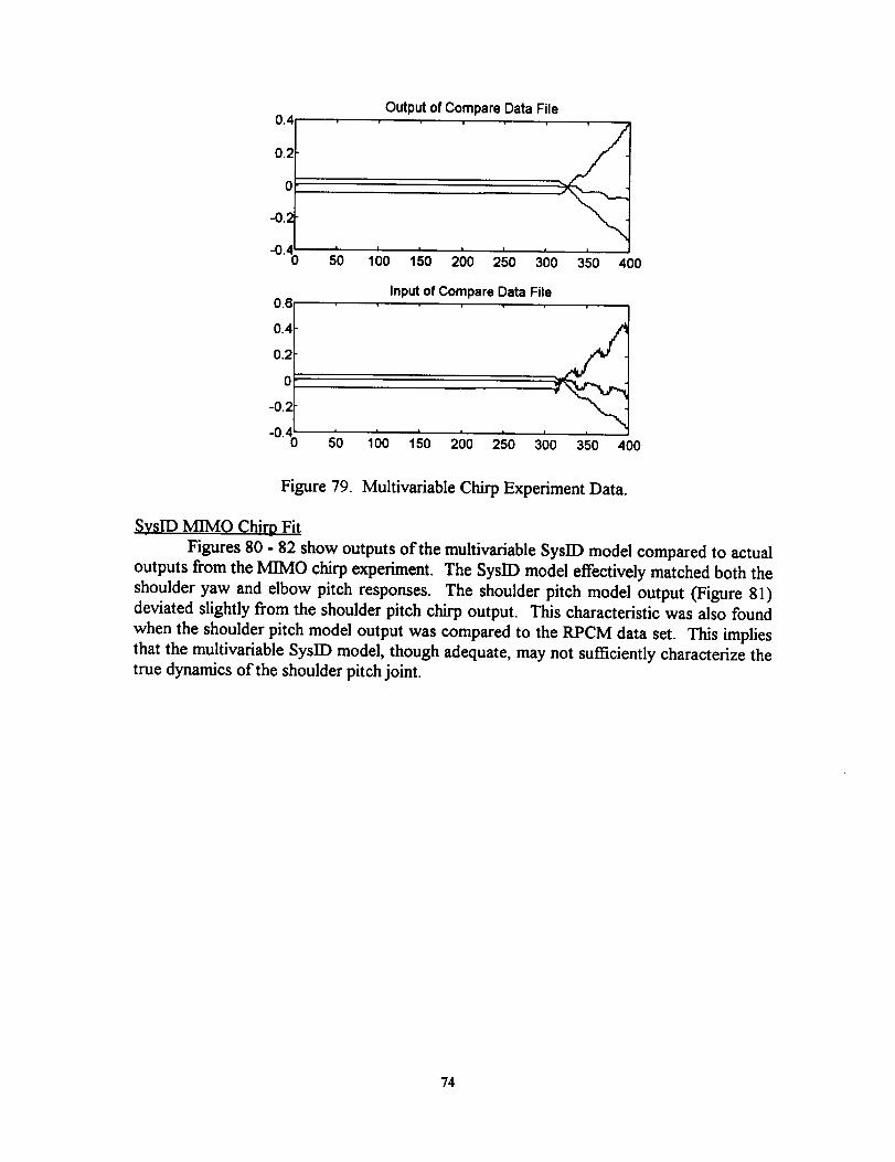
Outputof Compare Data File0.4
O,
•-(_014' , i , , , , , I
0 50 100 150 200 250 300 350 400
0.6Inputof CompareData File
0.4
0.2
0
-0.:
-el I I I I /
50 100 150 200 250I
300 350 400
Figure 79. Multivariable Chirp Experiment Data.
SyslD MIMO Chirp Fit
Figures 80 - 82 show outputs of the multivariable SysID model compared to actual
outputs from the M]MO chirp experiment. The SyslD model effectively matched both the
shoulder yaw and elbow pitch responses. The shoulder pitch model output (Figure 81)deviated slightly from the shoulder pitch chirp output. This characteristic was also found
when the shoulder pitch model output was compared to the RPCM data set. This implies
that the multivariable SysID model, though adequate, may not sufficiently characterize the
true dynamics of the shoulder pitch joint.
74
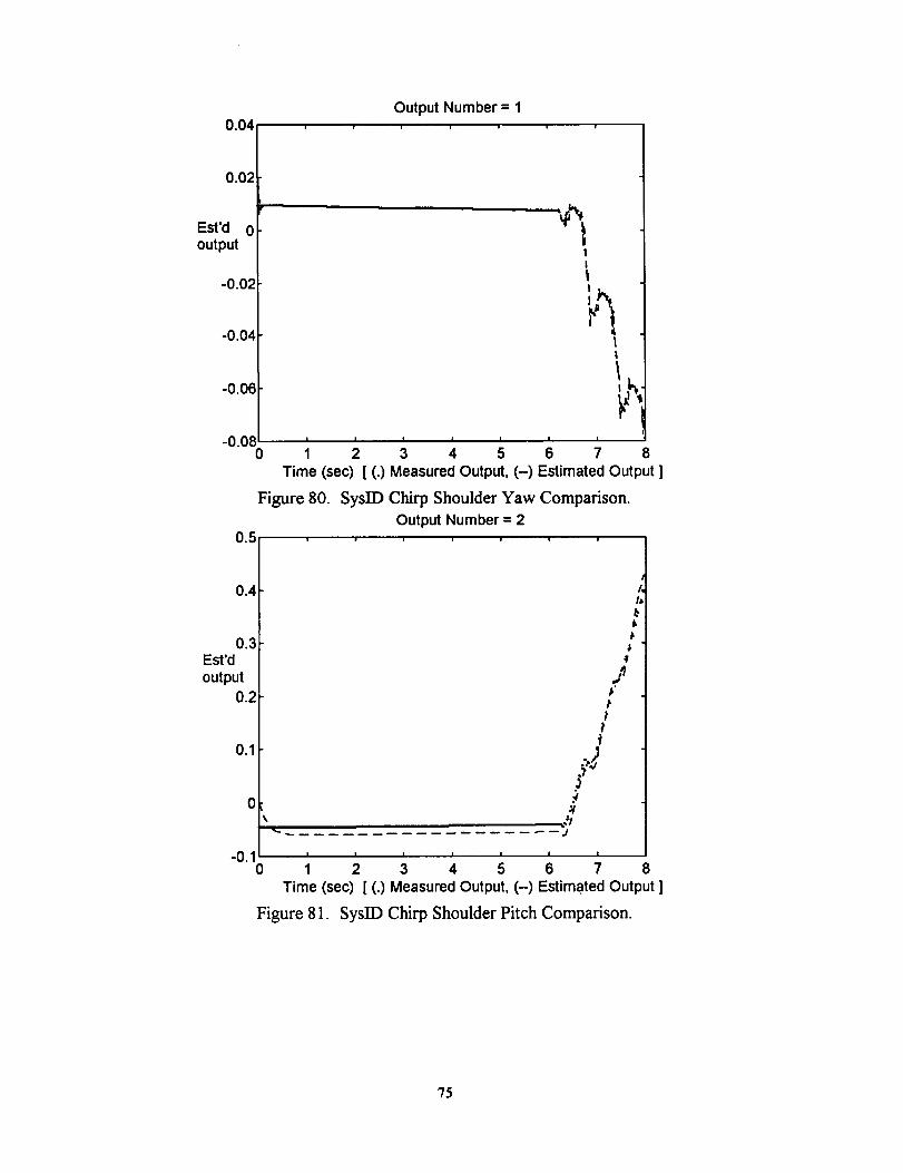
0.04Output Number = 1
0.02
Est'd 0output
-0.02
-0.04
1!t
I
|
-0.080 1 2 3 4 5 6 7 8
Time (sec)[ (.) Measured Output, (--) Estimated Output ]
Figure 80. SysID Chirp Shoulder Yaw Comparison.
Output Number = 20.5 .......
0.4
0.3Est'doutput
0.2
0.1
-0.10
t
/,
l=
I I I I I
1 2 3 4 5 8
t
)
d
| !
6 7
Figure 81.
Time (sec)[ (.) Measured Output, (--) Estimated Output ]
SysID Chirp Shoulder Pitch Comparison.
75
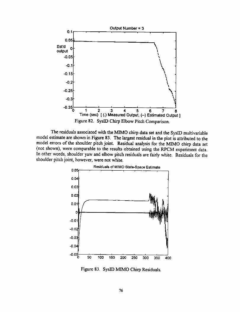
0.1
,0"051
Est d 0 koutput |
/
-0.05
-0.1
-0.15
-0.2
-0.25
-0.3
-0.350
Figure 82.
Output Number = 3i • n i
\tt
\\
!11
Time (sec) [ (.) Measured Output, (-) Estimated Output ]
SysID Chirp Elbow Pitch Comparison.
The residuals associated with the MIMO chirp data set and the SysID multivariable
model estimate are shown in Figure 83. The largest residual in the plot is attributed to the
model errors of the shoulder pitch joint. Residual analysis for the MIMO chirp data set
(not shown), were comparable to the results obtained using the RPCM experiment data.
In other words, shoulder yaw and elbow pitch residuals are fairly white. Residuals for the
shoulder pitch joint, however, were not white.
0.0!Residuals of MIMO State-Space Estimate
0.010
-0.01
-0.(
-0.0
i = i
50 100 150 200 250 300 350 400
Figure 83. SysID MIMO Chirp Residuals.
76
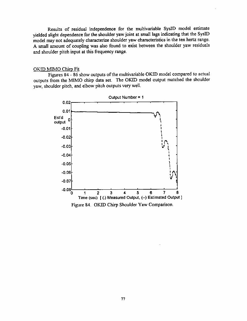
Results of residual independence for the multivariable SysID model estimate
yielded slight dependence for the shoulder yaw joint at small lags indicating that the SysID
model may not adequately characterize shoulder yaw characteristics in the ten hertz range.
A small amount of coupling was also found to exist between the shoulder yaw residuals
and shoulder pitch input at this frequency range.
OKID MIMO Chirp Fit
Figures 84 - 86 show outputs of the multivariable OKID model compared to actual
outputs from the MIMO chirp data set. The OKID model output matched the shoulder
yaw, shoulder pitch, and elbow pitch outputs very well.
Output Number = 10.02 , , ,
0.01
Est'd 0output
-0.01
-0.02
-0.03
-0.04
-0.05
-0.06 I
ozI0
! |
1 2Time (sec)
Figure 84.
I1It
!
|4I
!1|
INV
! , , , , ]
3 4 5 6 7 8[ (.) Measured Output, (-) Estimated Output ]
OKID Chirp Shoulder Yaw Comparison.
77
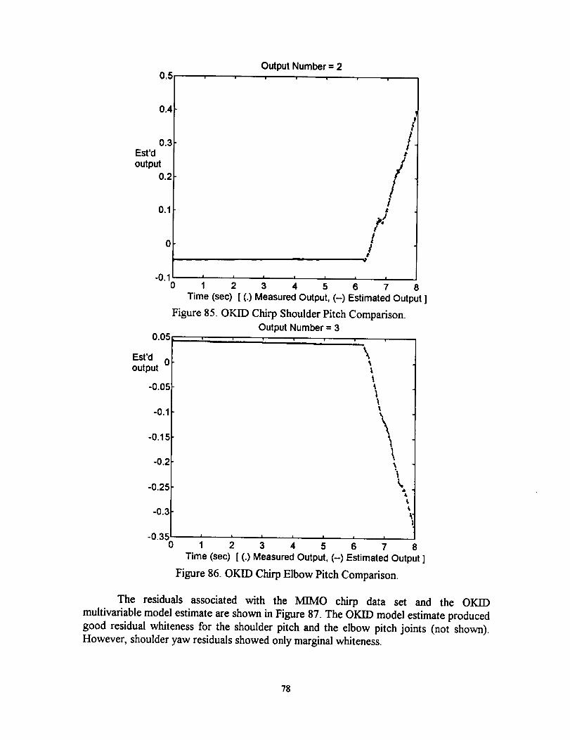
0.5Output Number = 2
i . v
0.4
0.3Est'doutput
0.2
0.1
0
-0.10
i
/4,
J
/!t
t
P/t
, 0.05Est d 0output
-O.OE
-0.1
-0.15
-0.2
-0.25
-0.3,-0.35 j
0
i I I i I I I
1 2 3 4 5 6 7 8Time (sec) [ (.) Measured Output, (-) Estimated Output ]
Figure 85. OKID Chirp Shoulder Pitch Comparison.
Output Number = 3, ! J | w t
\t
t
1!i
\I,
, t7 8
i i I I I I
1 2 3 4 5 6
Time (sec) [ (.) Measured Output, (--) Estimated Output ]
Figure 86. OKID Chirp Elbow Pitch Comparison.
The residuals associated with the MIMO chirp data set and the OKID
multivariable model estimate are shown in Figure 87. The OKID model estimate produced
good residual whiteness for the shoulder pitch and the elbow pitch joints (not shown).
However, shoulder yaw residuals showed only marginal whiteness.
78
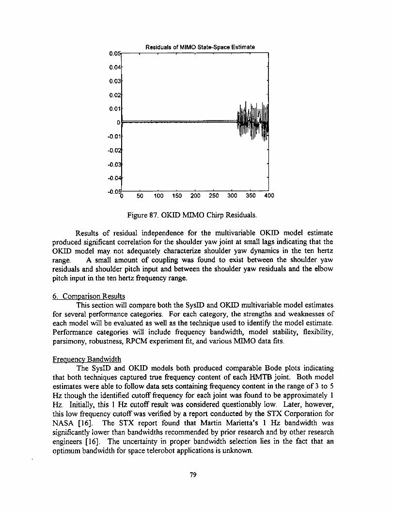
0.0_
0.04
0.02
0.02
0.01
0
-0.01
-0.01
-0.0_
-0.0_
-0.0._
Residuals of MIMO State-Space Estimate
I & I i I I I
50 100 150 200 250 300 350 400
Figure 87. OKID MIMO Chirp Residuals.
Results of residual independence for the multivariable OKID model estimate
produced significant correlation for the shoulder yaw joint at small lags indicating that the
OKID model may not adequately characterize shoulder yaw dynamics in the ten hertz
range. A small amount of coupling was found to exist between the shoulder yaw
residuals and shoulder pitch input and between the shoulder yaw residuals and the elbow
pitch input in the ten hertz frequency range.
6. Comparison Results
This section will compare both the SysID and OKID multivariable model estimates
for several performance categories. For each category, the strengths and weaknesses of
each model will be evaluated as well as the technique used to identify the model estimate.
Performance categories will include frequency bandwidth, model stability, flexibility,
parsimony, robustness, RPCM experiment fit, and various MIMO data fits.
Frequency Bandwidth
The SyslD and OKID models both produced comparable Bode plots indicating
that both techniques captured true frequency content of each HMTB joint. Both model
estimates were able to follow data sets containing frequency content in the range of 3 to 5
Hz though the identified cutoff frequency for each joint was found to be approximately 1
Hz. Initially, this 1 Hz cutoff result was considered questionably low. Later, however,
this low frequency cutoff was verified by a report conducted by the STX Corporation for
NASA [16]. The STX report found that Martin Marietta's 1 Hz bandwidth was
significantly lower than bandwidths recommended by prior research and by other research
engineers [16]. The uncertainty in proper bandwidth selection lies in the fact that an
optimum bandwidth for space telerobot applications is unknown.
79

When compared to data sets containing a greater than 5 Hz frequency content, the
OKID estimate slightly outperformed the SyslD estimate for each joint. This may have
been attributed to inadequate modeling of the SyslD estimate.
Stability
Since the magnitude of the eigenvalues for both multivariable model estimates
were less than unity, both models were found to be stable.
Flexibility
In terms of flexibility, the prediction error techniques used to determine the SysID
model estimate provided numerous approaches to model both the dynamics of the system
as well as the noise properties of the HMTB joints. The OKID technique, though moreaccurate, was less flexible.
Parsimony
The Observer/Kalman filter identification (OKID) technique was more
parsimonious in its attempt to describe the dynamic characteristics of the HMTB joints.
Information extracting using this technique produced a minimum realization in allowing
each joint to be described by a second-order system. In contrast, the SysID model used a
fifth-order model to describe the shoulder yaw dynamics, a second-order model to
describe the shoulder pitch dynamics, and a third-order model to describe the elbow pitchdynamics.
Robustness of estimates
The SyslD model proved to be more robust when compared to the OKID model
estimate. Comparable SysID models were obtained even in the presence of bias errors and
outliners in the data set. For instance, data detrending and/or filtering reduced a particular
SyslD model from a third-order system to a second-order system. In contrast, the OKID
estimate was more sensitive to bias errors and outliners in the data set. One OKID model
required a fourth-order system to describe the dynamics of a joint. However, a second-order model was sufficient when the data set was detrended.
RPCM Experiment Fit
The OKID multivariable model estimate provided a much better fit when
compared to data obtained from the RPCM experiment. The OKID estimate obtained a
more accurate fit by effectively minimizing the residuals for each joint model. The
identified model showed minimal coupling between the joints in the localized region. The
SyslD model estimate consistently showed high residuals for the shoulder pitch SISO
estimate. This can be attributed to the OE model structure used to characterize the joint.
MIMO Data Fits
The OKID estimate produced a better fit when compared to a majority of MIMO
data sets. For low frequency data sets, the SysID estimate modeled the dynamics of the
shoulder yaw joint much better than the OKID estimate. This would imply perhaps a
hybrid model between the OKID estimate (shoulder pitch and elbow pitch) and the SysID
80

estimate(shoulderyaw) to providean overallbettermultivariablemodelestimatefor lowfrequencies.
Overall, the Observer/Kalmanfilter identification(OKID) techniqueproduced a bettermultivariableestimatewhencomparedto the SysIDmultivariablemodelestimate. Menu-driven sottwarewas developedandusedto evaluatethe OKID model and to comparebothmultivariablemodels.
81

Vll Conclusions
Linear, dynamic models for three joints of the hydraulic manipulator test bed
(HMTB) at the NASA Langley Research Center have been identified using nonparametric
and parametric system identification techniques. Nonparametric techniques yielded an
approximate 1 Hz bandwidth for each joint using transfer function analysis, an expectedorder for each joint using correlation analysis, and the degree of process and measurement
disturbances for each joint using spectral analysis. Two different parametric identification
techniques were used and compared in developing dynamic models of the joints. The first
parametric technique, used primarily for control system identification, employed aprediction-error method to produce a stable model estimate. The bandwidth for this
estimate proved adequate when compared to several data sets. An advantage of thistechnique is its flexibility of use. The user has several options, alternatives, and methods
from which to conduct an identification investigation. When compared to the RPCM
experiment data, this technique yielded adequate results. The second parametrictechnique, used primarily in modal system identification, employed a minimum realization
algorithm to produce a stable model estimate using only second-order systems to describe
the characteristics of each joint. This technique was extremely simple to use while yet
providing an adequate bandwidth for the identified models among many data sets. Themodels identified using this technique produced an accurate fit to both the RPCMexperiment data and various MIMO data sets.
Matlab menu-driven system identification software scripts were developed for this
thesis. One program, using functions from the MA TI__B System Identification Toolbox,
was used to perform nonparametric and parametric analysis of the manipulator data. The
other program identified models using the Observer/Kalman Filter Identification (OKID)technique, provided in the System/Obse_er/Controller Identification Toolbox (SOCIT).
The latter program used several toolboxes to perform MIMO comparisons for the
identified multivariable models. Both programs were found to be extremely useful
especially in minimizing the time required to perform nonparametric and parametric
analysis of the data. The programs, modular in design, are easily expandable. Though
written to use data from the manipulator joints, the programs may be easily adapted toincorporate data from any dynamic system for the purpose of identification.
1. Suggestions for Future Work
With the identified models in this investigation valid only in a localized region witha specific loading, additional identification tests should be performed. Recursive
identification methods, in particular, should be performed with several different loading
configurations for the manipulator. Also, a more complete model should be identified bydetermining the dynamic parameters of the shoulder roll, wrist pitch, wrist yaw, and wristroll joints (which were not identified in this thesis).
2. Model Reference Control
A model reference control system is proposed for the previously identified
multivariable dynamic HMTB model. In this controls approach, the behavior of the
ground-based model would closely resemble the behavior of the on-orbit flight model for
82
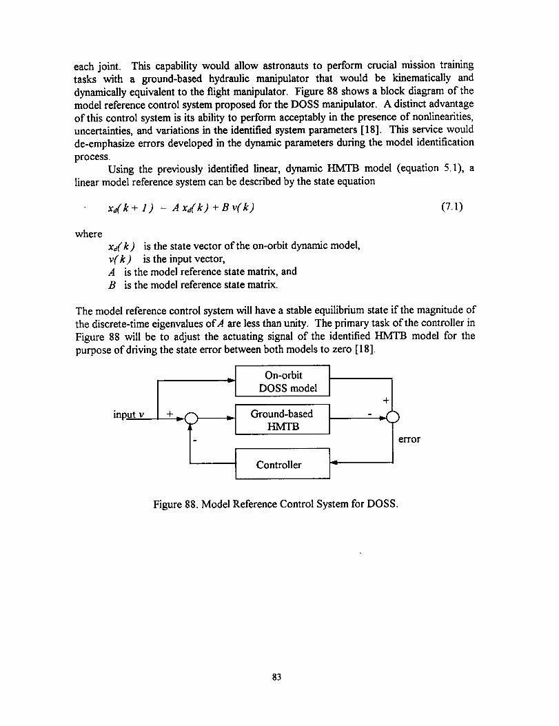
each joint. This capability would allow astronauts to perform crucial mission training
tasks with a ground-based hydraulic manipulator that would be kinematically and
dynamically equivalent to the flight manipulator. Figure 88 shows a block diagram of the
model reference control system proposed for the DOSS manipulator. A distinct advantage
of this control system is its ability to perform acceptably in the presence of nonlinearities,
uncertainties, and variations in the identified system parameters [18]. This service would
de-emphasize errors developed in the dynamic parameters during the model identification
process.
Using the previously identified linear, dynamic HMTB model (equation 5.1), a
linear model reference system can be described by the state equation
xa(k + l) = Axa(k) + Bv(k) (7.1)
where
xd(k) is the state vector of the on-orbit dynamic model,
v(k) is the input vector,
A is the model reference state matrix, and
B is the model reference state matrix.
The model reference control system will have a stable equilibrium state if the magnitude of
the discrete-time eigenvalues of A are less than unity. The primary task of the controller in
Figure 88 will be to adjust the actuating signal of the identified HMTB model for the
purpose of driving the state error between both models to zero [18].
input v
P[ On-orbitDOSS model
+ _ __ _ Ground-based
Controller
+
- _()
error
Figure 88. Model Reference Control System for DOSS.
83
References
[1]
[2][3]
[4]
[5]
[6][7]
[8]
[9]
[lO]
[11]
[12]
[13]
[14]
[15]
[16]
[17]
[18]
[19]
Kohrs, Richard H., "Freedom is an International Partnership," Aerospace America.September 1990.
Fisher, Arthur., "NASA's New Direction," Popular Science, March 1991.
Summary and Principal Recommendations of the Advisory Committee on the
Future of the U.S. Space Program. NASA Headquarters, December 10, 1990.
Lawler, A. and Knapp, B., "Canadian Station Role Revised," Space News.April 25-May 1, 1994.
Flight Telerobotic Servicer (FTS) Requirements Document for Phase C/D.
NASA SS-GSFC-0043, September 1990.
FTS-Trainer Design Review Data Package. WSM E91/004, March 1, 1991.
MSS On-Orbit Operations Concept Document, Vol. 2. SPAR-SS-R0444,December 1992.
Juang, Jer-Nan., Applied System Identification. Prentice-Hall, EnglewoodCliffs, New Jersey, 1994.
Soderstrom, T., and Stoica, P., System Identification. Prentice-Hall, EnglewoodCliffs, New Jersey, 1989.
Ljung, L., System Identification: Theory for the User. Prentice-Hall, EnglewoodCliffs, New Jersey, 1987.
Juang, J.-N., and Pappa, R. S., "A Comparative Overview of Modal Testingand System Identification for Control of Structures." Shock and Vibration
Digest, Vol. 20, No. 5, May 1988, pp. 4-15.
Ho, B. L. and Kalman, R. E., "Effective Construction of Linear State Variables
Models from Input/Output Data," Proceedings of the 3rdAnnual Allerton
Conference on Circuit and System Theory, pp. 449-459, 1965.
Ha, T. T. and Pratt, T., Study of Spread Spectrum Multiple Access Systems
for Satellite Communications with Overlay on Current Services,NASA CR-180827, 1987.
Franklin, G. F., Powell, J. D., and Workman, M. L., Digital Control of DynamicSystems. Second Edition. Addison-Wesley, 1990.
AT-M10-16 User Manual National Instruments Corporation, Part Number320476-01, 1992.
Brooks, T.L., Telerobot Response Requirements. STX Corporation. ReportNumber STX/ROB/90-03. March 1990.
Shattuck, P. L. and Lowrie, J. W., "Flight Telerobotic Servicer Legacy."
Cooperative Intelligent Robotics in Space 111, Vol. 1829, 1992, pp. 60-74.
Ogata, K., Modern Control Engineering. Second Edition. Prentice-Hall,
Englewood Cliffs, New Jersey, 1990.
Juang, J.-N., Horta L., and Phan M., System�Observer�Controller
Identification Toolbox (SOCIT). NASA TM-107566. February 1992.
84

Appendix A. Plots and Graphs
This appendix contains plots and graphs for the shoulder pitch and elbow pitch
joints. Explanation of the graphs are discussed in the main text. The graphs and plots are
divided into three subdivisions as follows:
A.1
A.2
A.3
Nonparametric PlotsClassical Parametric Plots
OKID Parametric Plots.
85
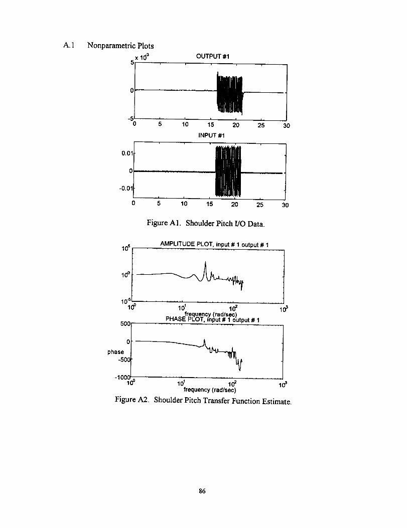
A1 Nonparametric Plots
x Id 35
o
OUTPUT #1
i
ii' 1,0 I ' 2'"% 5 15 20 5
INPUT #1
0 5 10
3O
15 20 25 30
Figure AI. Shoulder Pitch I/O Data.
105 AMPLITUDE PLOT, input # 1 output # 1
lO0
1O1oO
500
0
phase-500
-100_0o
Figure A2
lo' lo_ o3frequency (radlsec)
PHASE PFOT, input # 1 output # 1
10' 102 103frequency (rad/sec)
Shoulder Pitch Transfer Function Estimate.
86
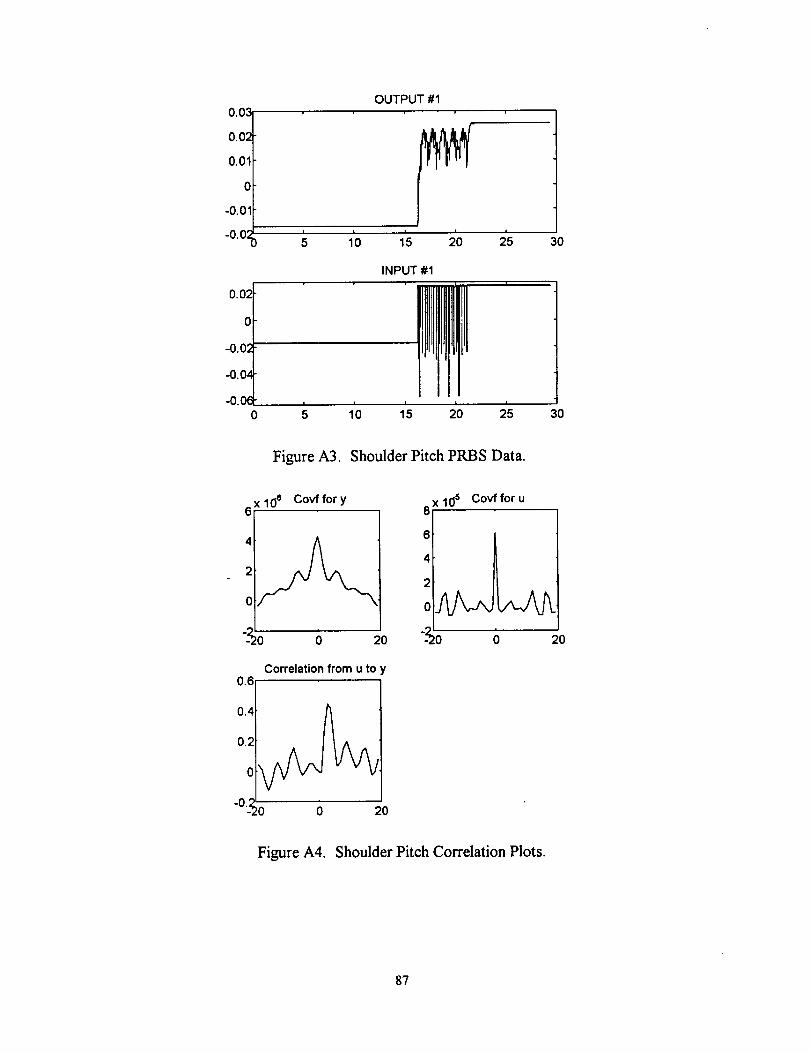
0.03
0.0;
0.01
0
-0.01
OUTPUT #1
-0.0 5 10 15 20 25 30
0.02
0
-0.02
-0.04
-0.060
INPUT #1
' ' ' 2"0 '5 10 15 25 30
Figure A3. Shoulder Pitch PRBS Data.
6xlOe Covffory 8x1_ Covfforu
0 2O 0
Correlation from u to y
0 20
6
4
2
0
20
Figure A4. Shoulder Pitch Correlation Plots.
87
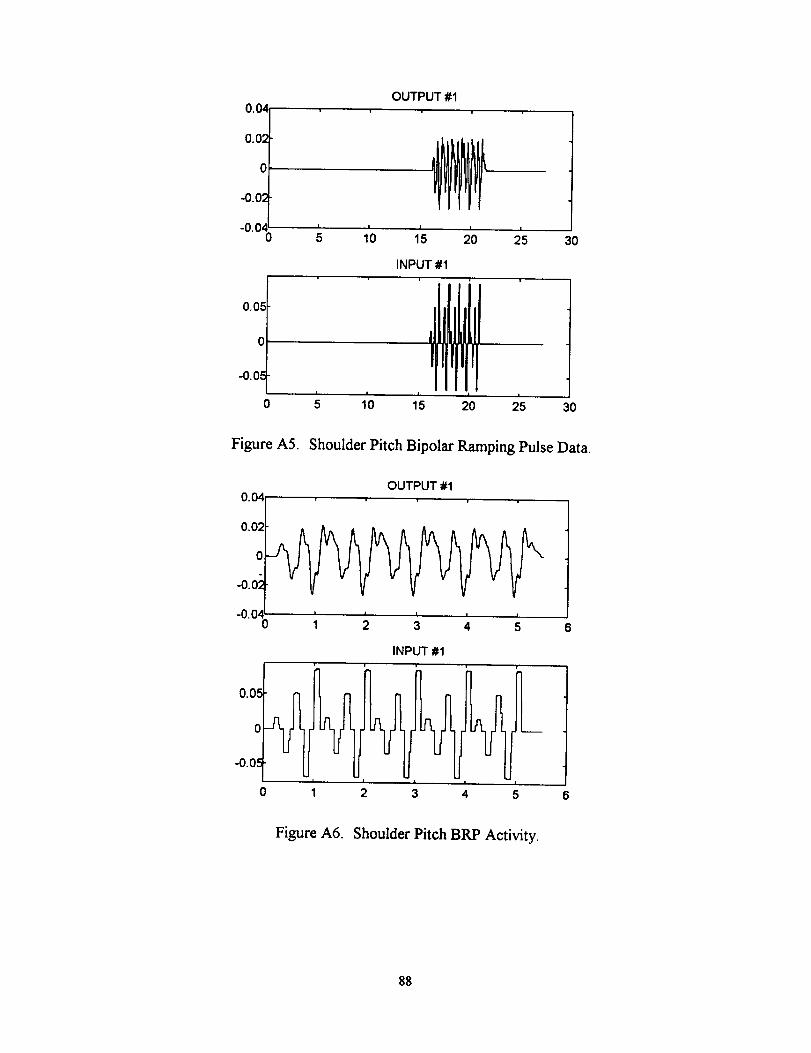
0.04
0.02
0
-0.02
-0.040
0.05
0
-0.05"
0
OUTPUT #1
; ;o l's 2'5 30INPUT #1
I I I I I
5 10 15 20 25 30
Figure A5. Shoulder Pitch Bipolar Ramping Pulse Data.
0.04
0.02
0
-0.0_
-0.040
0.05
o2_,I#
-0.0.=
0
OUTPUT #:1
1 2 5 6
INPUT #1
1 2 3 4 5
Figure A6. Shoulder Pitch BRP Activity.
88
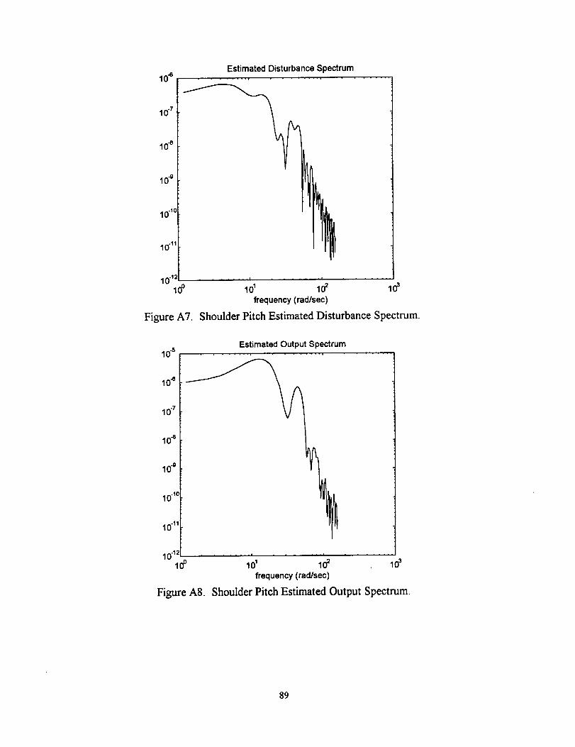
10"s
10.7
10"8
10"g
10"lc
10"_
Figure A7.
Estimated Disturbance Spectrum
.... J ,i •
101 103 103
frequency(rad/sec)
Shoulder Pitch Estimated Disturbance Spectrum.
10.5
lO_
10.7
lO_
10-e
10-lo
10-11
10-12lO0
Figure A8.
Estimated Output Spectrum
101 102 103
frequency (rad/sec)
Shoulder Pitch Estimated Output Spectrum.
89
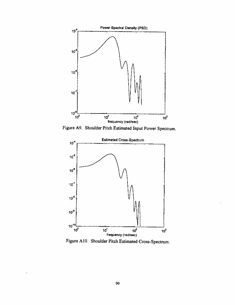
104
lO-'
10"e
10.7
Figure A9.
IO_
Power Spectral Density (PSD)....... , ...... ,
.... i
10' 10= 103
frequency (rad/sec)
Shoulder Pitch Estimated Input Power Spectrum.
Estimated Cross-Spectrum
10-s
I
10-e
10.7
10-s
10.9
101° --loo lo_ lo_
frequency (rad/sec)
Figure A10.
lO'
Shoulder Pitch Estimated Cross-Spectrum.
9o
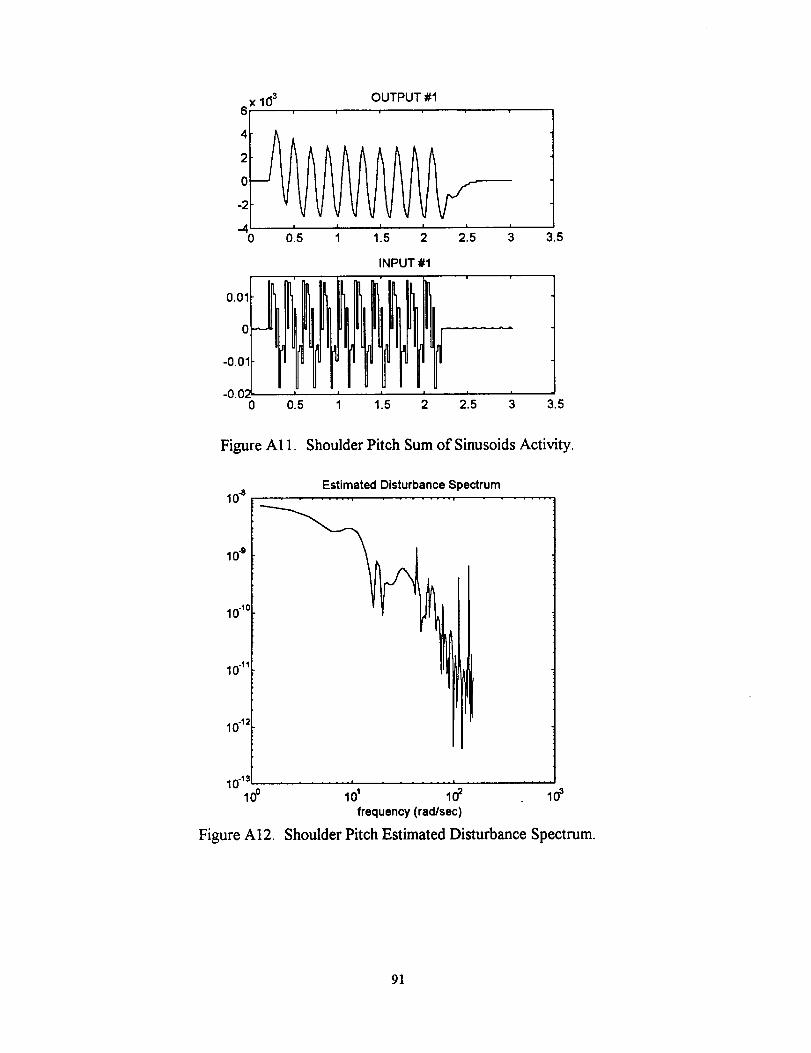
6x 1(33 OUTPUT #1
4
2
0
-2
I"o 1.s I
2.5I
3 3.5
0.01
0
-0.01
-0.02-0
INPUT #1
I I I I I I
0.5 1 1.5 2 2.5 3 3.5
Figure AI 1. Shoulder Pitch Sum of Sinusoids Activity.
lo_
10"°
10-lo
10-11
10-12
Estimated Disturbance Spectrum
10-13 .... - .................lo0 lo' lo= lO'
frequency (rad/sec)
Figure A12. Shoulder Pitch Estimated Disturbance Spectrum.
91
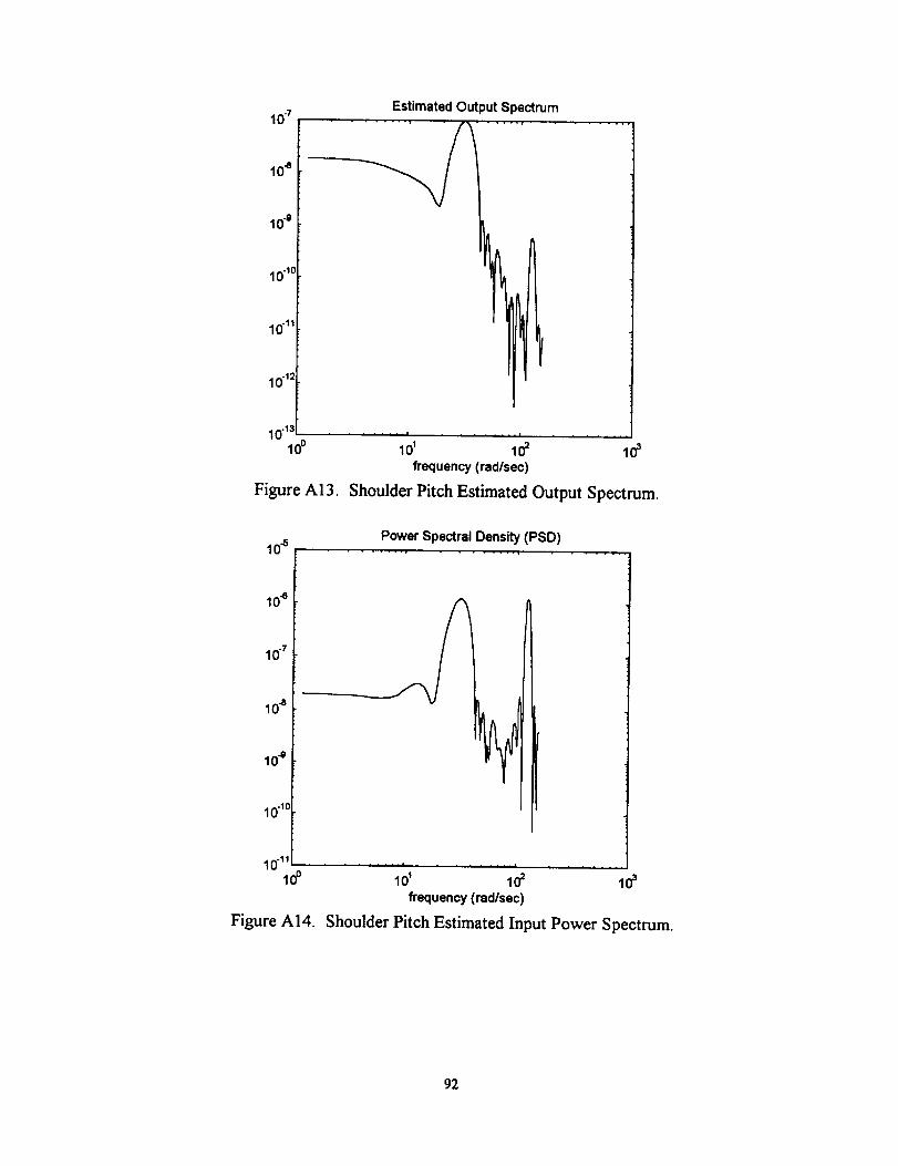
10.7
IO_
10 "9
10 "to
10-'1
10 1;
10 .'3lO0
EstimatedOutput Spectrum
..... . . . .=
lO' lO_ 1#frequency (rad/sec)
Figure A] 3 Shoulder Pitch Estimated Output Spectrum
10 -sPowerSpectralDensity(PSD)
lO_
10 .7
10 "s
lO_
10 "1o
10 ''1
lO0.I .... i
10' 102 I0s
frequency (rad/sec)
Figure AI4. Shoulder Pitch Estimated Input Power Spectrum.
92
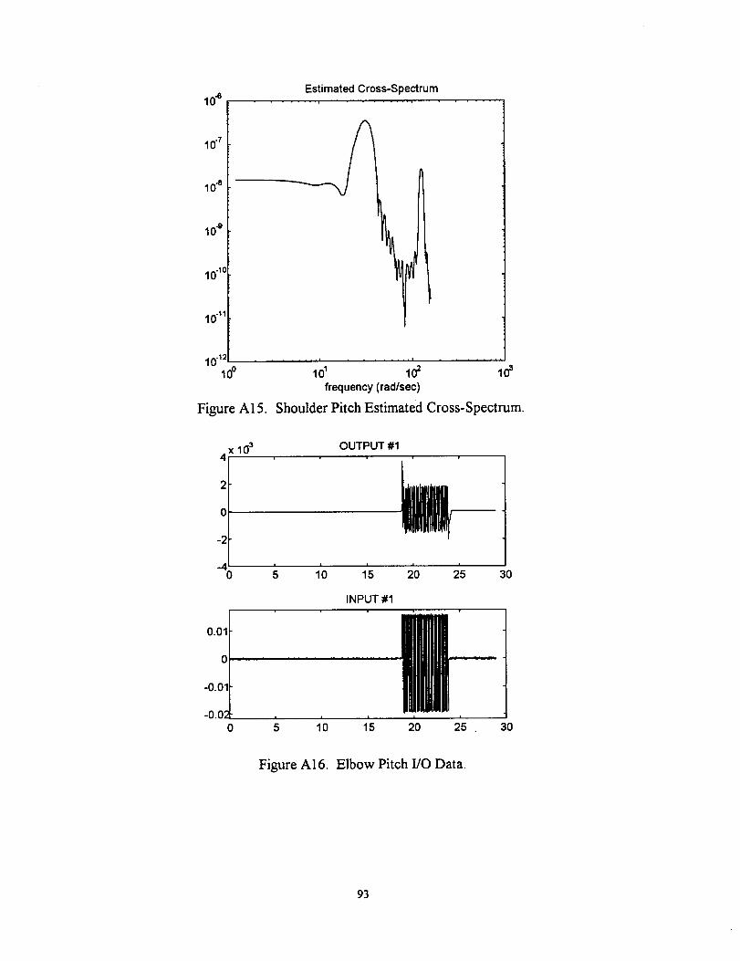
Estimated Cross-Spectrum10"8 ....... , ........
10.7
lO_
10.9
10"10
10-11
101; ...........lOo lOI lO_ lO3
frequency (rad/sec)
Figure A15. Shoulder Pitch Estimated Cross-Spectrum.
X 103 OUTPUT #14
2
0
-2
..d
0 I | i I10 15 20 25 30
0.01
0 ' ' '
-0.01
-0.02I
0 5
INPUT #1
I I
10 15 30I I
20 25
Figure AI6. Elbow Pitch I/O Data.
93
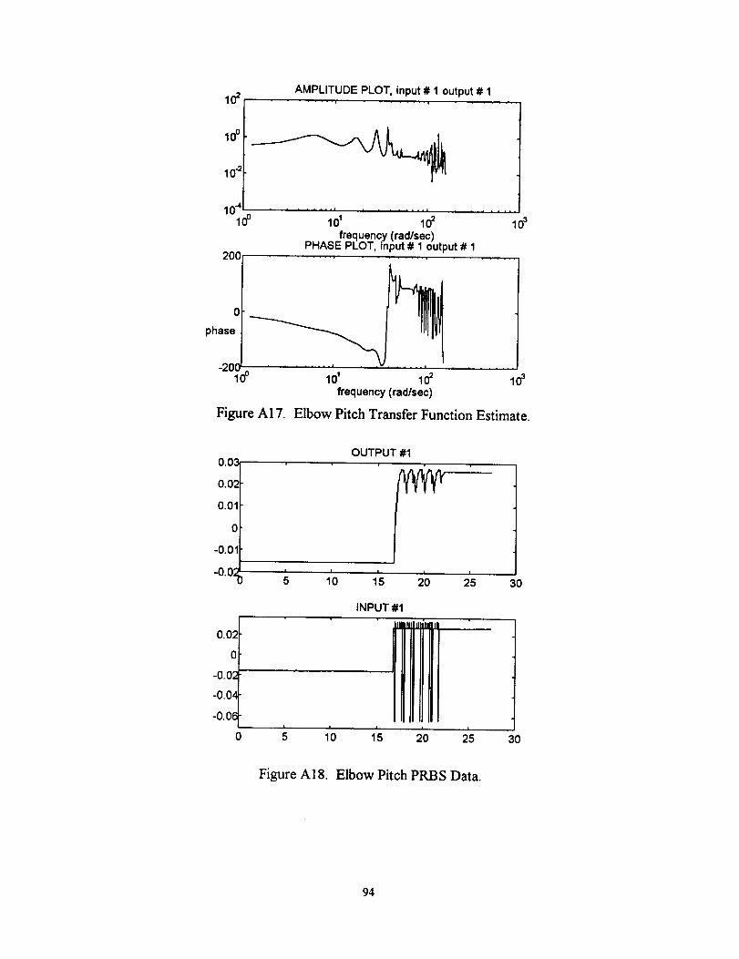
AMPLITUDE PLOT, input # 1 output # 110= .......
10-2
_oo ..........lO lO' 10=frequency (rad/sec)
PHASE PLOT, input # 1 output # 12OO
1@
0
phase
"201C0o
\101 lO=
frequency (rad/sec)
Figure A17.
lO_
Elbow Pitch Transfer Function Estimate.
0.03
0.02
0.01
0
-0.01
-0.0:
0.02
0
-0.02
-0.04
-0.06
0
OUTPUT #1
1'o 1's 2'o 2'_ 30
INPUT #1
| I | | I
5 10 15 20 25 30
Figure A18. Elbow Pitch PRBS Data.
94
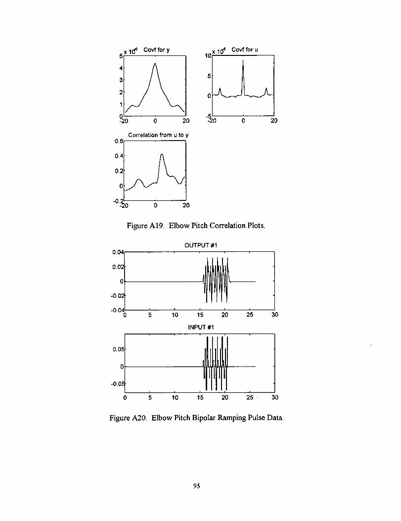
5x10 e Covffory
4
3
2:
q_o-d 20
Correlation from u to y
0 20
10x 10s Covf for u
5
0
-520 0 20
Figure A19. Elbow Pitch Correlation Plots.
0.04
0.02
0
-0.0,_
-0.0,_0
OUTPUT #1
! I; lo ;_ 2'0 2_ 3oINPUT #1
0.0_
0
-0.0,=
0I I I I I
5 10 15 20 25' 30
Figure A20. Elbow Pitch Bipolar Ramping Pulse Data.
95
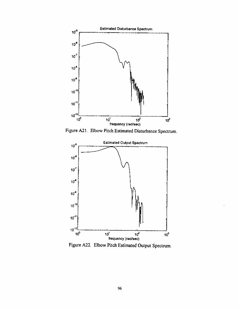
IO_
10.7
lO"
lo"
10-lc
10 -11
10 -1:lO0
Estimated Disturbance Spectrum
frequency (rad/sec)
Figure ._ ]. Elbow Pitch Estimated Disturbance Spectrum.
io_
10"
10 .7
lO"
10.9
10-1c
10"11
10-12lo0
Estimated Output Spectrum
1= • .i
101 102 103
frequency (rad/sec)
FiooureA22. Elbow Pitch Estimated Output Spectrum.
96
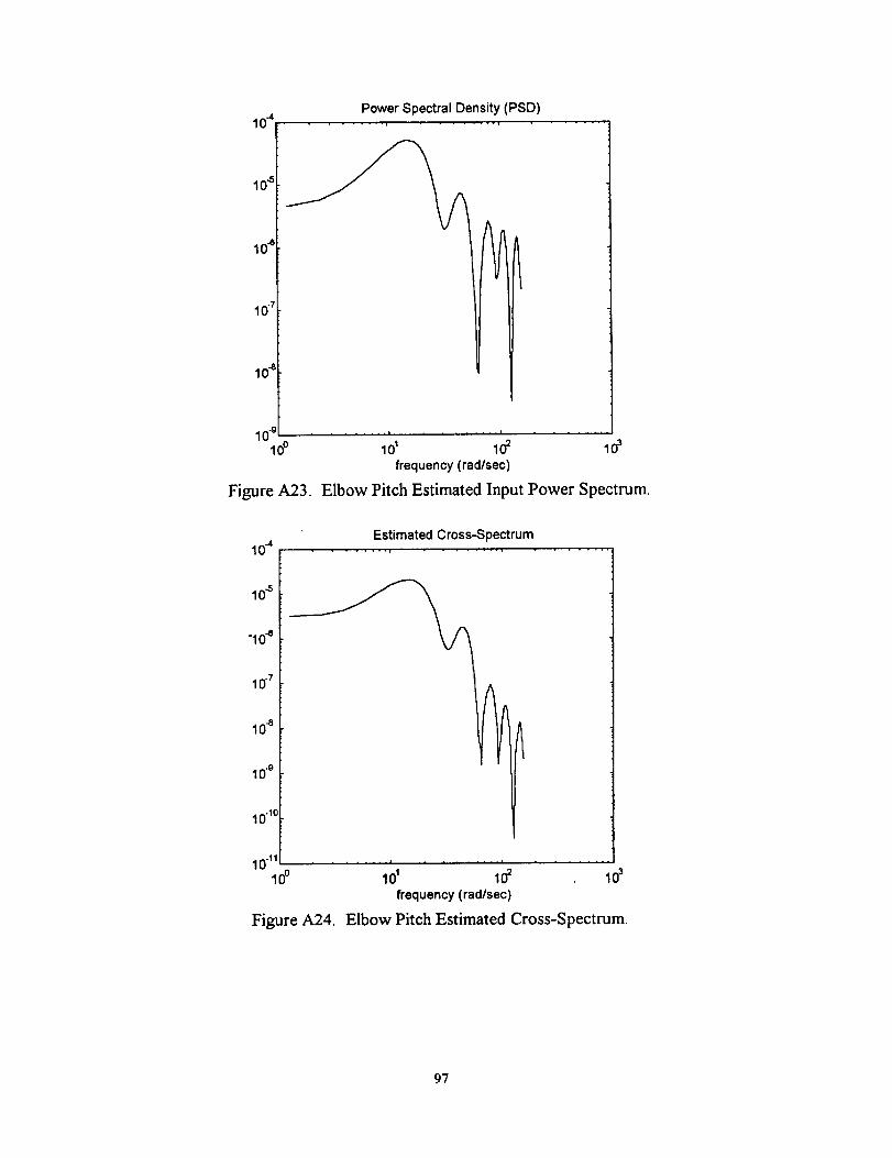
PowerSpectralDensity(PSD)10-4 ...... , ....... ,
lO_
lO_
10.7
10 .... ' ........ i
10o 101 102 103
frequency (rad/sec)
Figure A23. Elbow Pitch Estimated Input Power Spectrum.
Estimated Cross-Spectrum10 -4 ....... ,
lO_
-10_
10-7
IO•
Io*
10"1o
10"11lo0
, , , , .... , ..... i .
lo' lo_ lo_frequency (rad/sec)
Figure A24. Elbow Pitch Estimated Cross-Spectrum
97
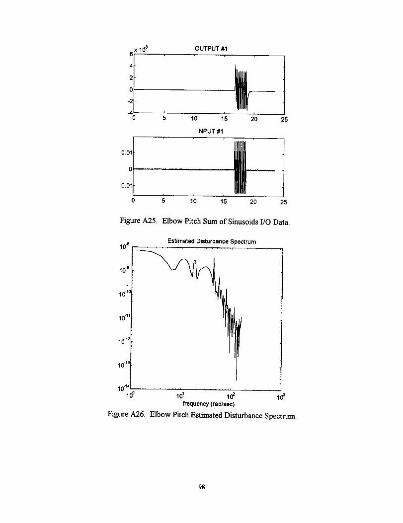
6X 10³OUTPUT #1
4
2
0
-2
-40 ' ' 1'55 10 25
I
20
0.01
0
-0.01
0
INPUT #1
i i
5 10 25i i
15 20
Figure A25. Elbow Pitch Sum of Sinusoids I/O Data.
10-a
10_
10-lo
10-11
10"12
10 "13
10 "14
lOo
Figure A26.
Estimated Disturbance Spectrum
I# 1# lO_frequency (rad/sec)
Elbow Pitch Estimated Disturbance Spectrum.
98
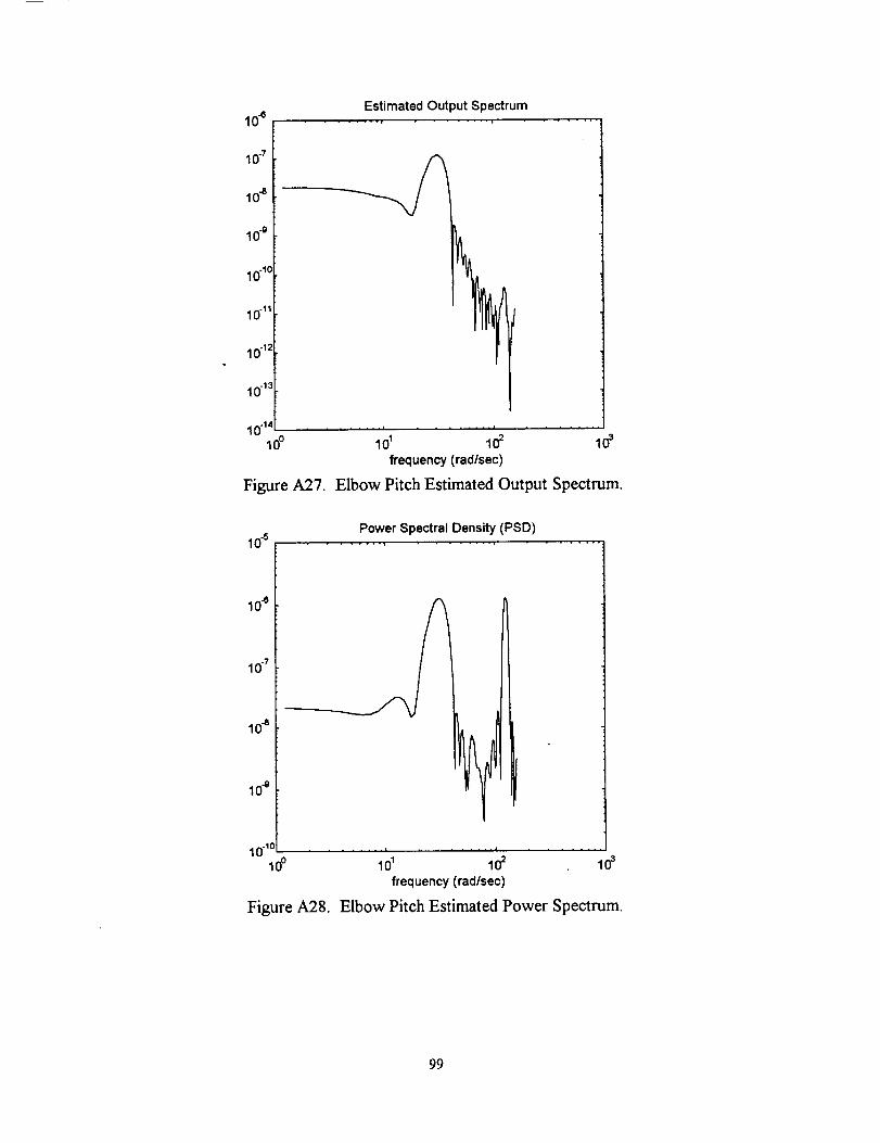
lO_
10 .7
10 -1_
10-1"=
10 "1:
10"1-_
10 -14
lO0
Figure A27.
Estimated Output Spectrum
.... , .... i
lO' lO_ lO_frequency (rad/sec)
Elbow Pitch Estimated Output Spectrum.
Power Spectral Density (PSD)10"s
10 8
10 .7
10 8
10 "g
10 "1c ............lO0 lo1 lO_
frequency (rad/sec)
Figure A28.
lO_
Elbow Pitch Estimated Power Spectrum.
99
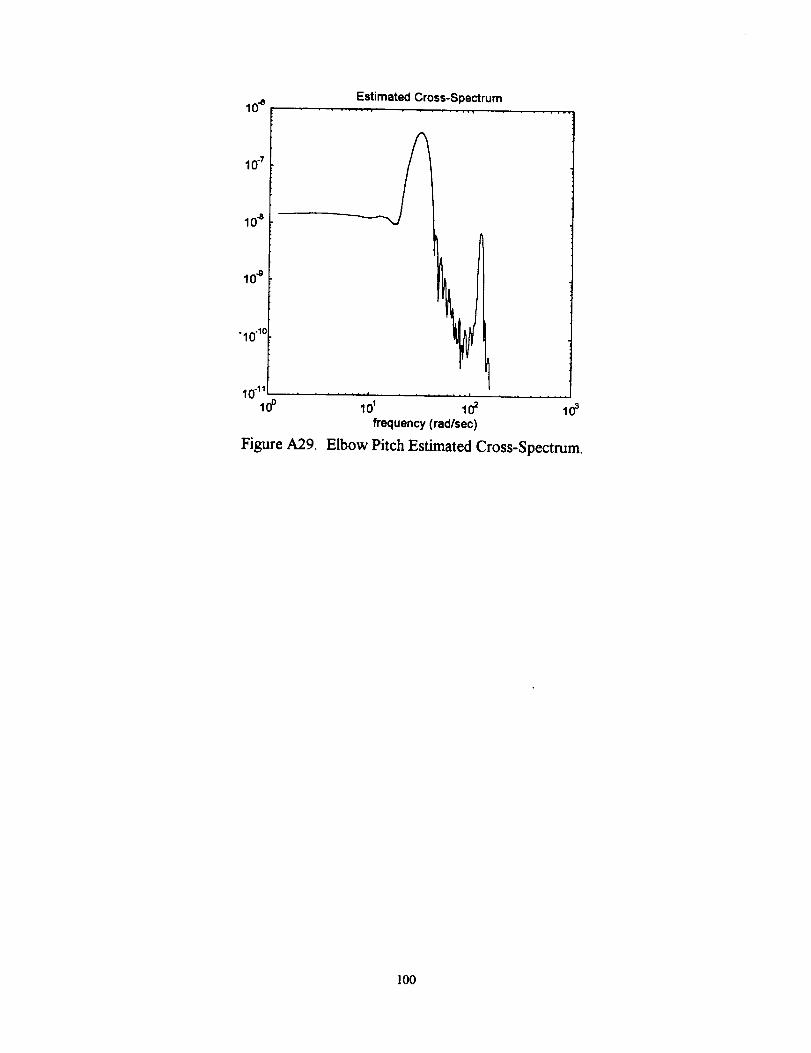
Estimated Cross-Spectrum104 ...............
10.7
10-e
•10-lc
Figure A29
lo' lo= lo'frequency (rad/sec)
Elbow Pitch Estimated Cross-Spectrum
lO0
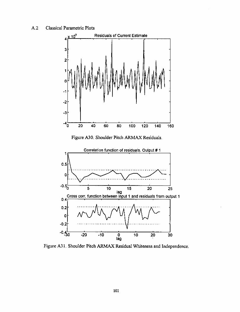
A.2 Classical Parametric Plots
4 x 10³ Residuals of Current Estimate
3
2
1
0
-1
-2
-3
-%
1' ' o'o ' ' 15o '20 40 80 100 140 160
Figure A30. Shoulder Pitch ARMAX Residuals.
Correlation function of residuals. Output # 1
0.5
0
-o.5; ; 1'o 1's 2'0 25lag
Cross corr. function between input I and residuals from out )ut I0.4
0.20-0.2
-o..% -:;o -,'o _ 1`0 2'o 30lag
Figure A31. Shoulder Pitch ARMAX Residual Whiteness and Independence.
101
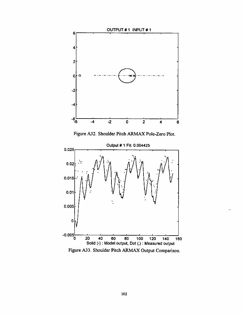
6
4
2
0 o
-2
-4
-6.6
OUTPUT # 1 INPUT # 1
I I / I !
-4 -2 0 2 4
Figure A32. Shoulder Pitch AKMAX Pole-Zero Plot.
0.025
0.02 " "
Output # 1 Fit: 0.004425
*o o
0.015
0.01 "
0.005
0
-0.0050 20 40 60 80 100 120 140 160
Solid (-) " Model output, Dot (.) • Measured output
Figure A33. Shoulder Pitch AR]VIAX Output Comparison.
102
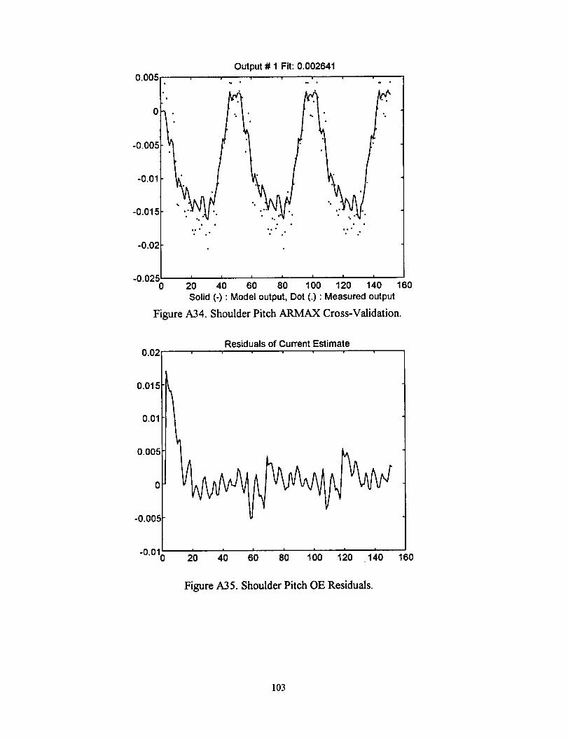
0.005
0
-0.005
-0.01
-0.015
"0"02t
-0.025 /0
Output # 1 Fit: 0.002641
o •
i
I i i I I I i
20 40 60 80 100 120 140 60Solid (-) • Model output, Dot (.) • Measured output
Figure A34. Shoulder Pitch ARMAX Cross-Validation.
0.02
0.015
0.01
0.005
0
-0.005
Residuals of Current Estimate
! I I-°°10 2'0 40 do 80 1;0 120 1;.0 160
Figure A35. Shoulder Pitch OE Residuals.
103
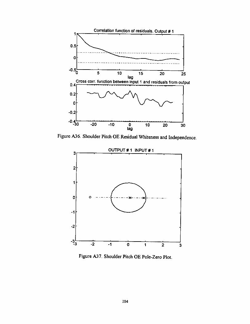
Correlation function of residuals. Output # 1
0.5 t.......
-0.50 5 10 15 20 25
lagCross corr. function between input I and residuals from output0,4 .................................................
0.20
-0.2
-o..% -_o ......-i'o.......o....... io.......2o" 30lag
Figure A36. Shoulder Pitch OE Residual Whiteness and Independence.
3
0
-1
-2
OUTPUT # 1 INPUT # 1
O
I I I3-3 -2 -1 _ 1 :; 3
Figure A37. Shoulder Pitch OE Pole-Zero Plot.
104
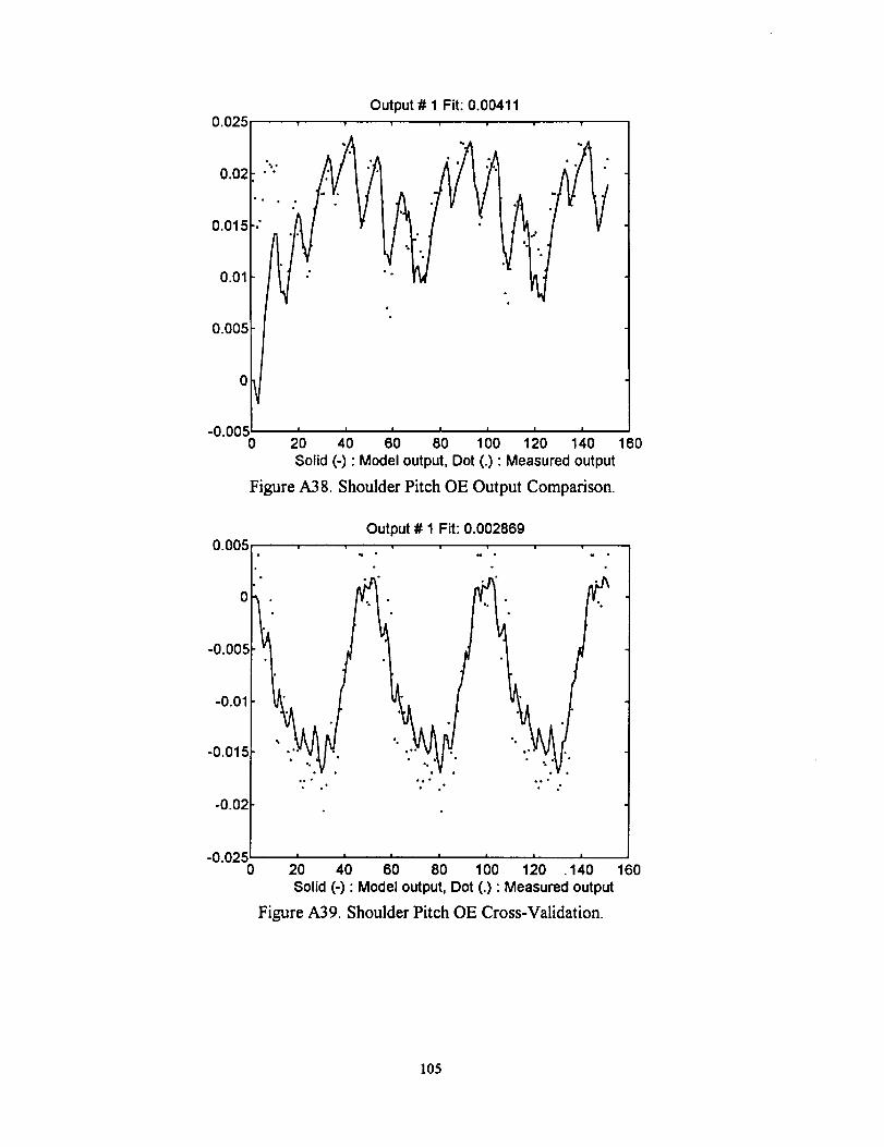
Output # 1 Fit: 0.004110.025
0.02
0.015
0.01
0.005
0
-0.0050 20 40 60 80 100 120 140 160
Solid (-) • Model output, Dot (.) • Measured output
Figure A38. Shoulder Pitch OE Output Comparison.
0.005
-0.005
-0.01
-0.015
-0.02
H°
Output # 1 Fit: 0.002869i
oQo •o•
-0.025 ' ' ' ' ' ' '0 20 40 60 80 100 120 .140 160
Solid (-) " Model output, Dot (.) • Measured output
Figure A39. Shoulder Pitch OE Cross-Validation.
105
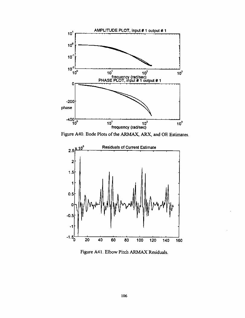
AMPLITUDE PLOT, input # 1 output # 1101 .............
10°
10-1
10-" ............10o 101 102
fre.quency (rad/sec).PHASE PLOT, input # 1 omput # 1
o°o phase /
.40000 .....101 102frequency (rad/sec)
10s
103
Figure A40. Bode Plots of the ARMAX, ARX, and OE Estimates.
x 1032.5
Residuals of Current Estimate
o-0.5
20 40 60 80 100 120 140 160
Figure A41. Elbow Pitch ARMAX Residuals.
106
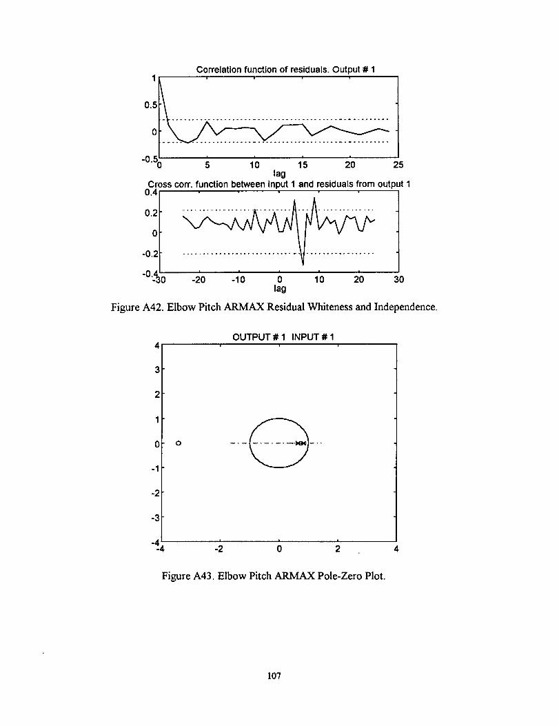
Correlation function of residuals. Output # 11
0.5
-o.5
, • I i
' ' 1"5 '5 10 20 25lag
Cross corr. function between input 1 and residuals from output 10.4
0.2
0
-0.2
-0..4_0I I I
-20 -10 0lag
I I
10 20 3O
Figure A42. Elbow Pitch ARMAX Residual Whiteness and Independence.
4
3
2
1
0
-1
-2
-3
-4
o
OUTPUT # 1 INPUT # 1
| I I
-2 0 2 4
Figure A43. Elbow Pitch ARMAX Pole-Zero Plot.
107
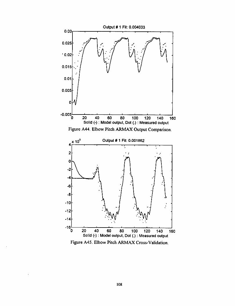
0.03Output # 1 Fit: 0.004003
0.01_
0.00_
0
-0.0050 20 40 60 80 100 120 140 160
Solid (-) • Model output, Dot (.) • Measured output
Figure A44. Elbow Pitch ARMAX Output Comparison.
xlo4
Output # 1 Fit: 0.001862
2
0
-2
-(
-8
-10
-12
-14
-160
." ... ."...._
• °° , •
20 40 60 80 100 120 140 160Solid (-) • Model output, Dot (.) • Measured output
Figure A45. Elbow Pitch _ Cross-Validation.
108
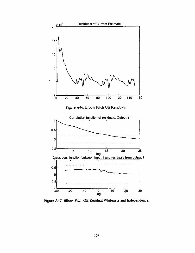
x ld 3 Residuals of Current Estimate20
15
10
5
0
"5O 160a i i i | i i
20 40 60 80 100 120 140
Figure A46. Elbow Pitch OE Residuals.
Correlation function of residuals. Output # 1
0.5
0
0 ! ! i I-0. 5 10 15 20 25lag
Cross corr. function between input 1 and residuals from output 11
0.5
0
-0.5
-.130 .....-20 -10 0 10 20 30lag
Figure A47. Elbow Pitch OE Residual Whiteness and Independence.
109
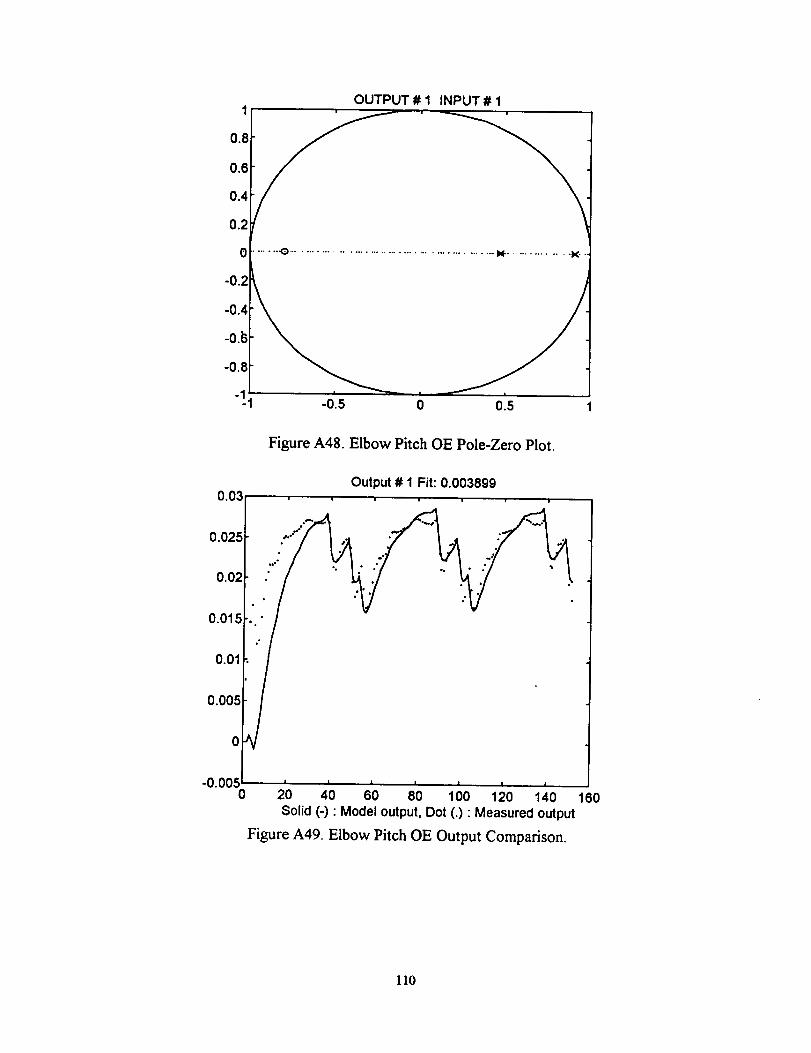
1
0.8
0.6
0.4
0.2
0
-0.2
-0.4
-0.t3
-0.8
-1
OUTPUT # 1 INPUT # 1
-0.5 0 0.5
Figure A48. Elbow Pitch OE Pole-Zero Plot.
Output # 1 Fit: 0.003899
0.025
0.01
0.01
0.005
-0.0050 20 40 60 80 100 120 140 160
Solid (-) "Model output, Dot (.) • Measured output
Figure A49. Elbow Pitch OF. Output Comparison.
110
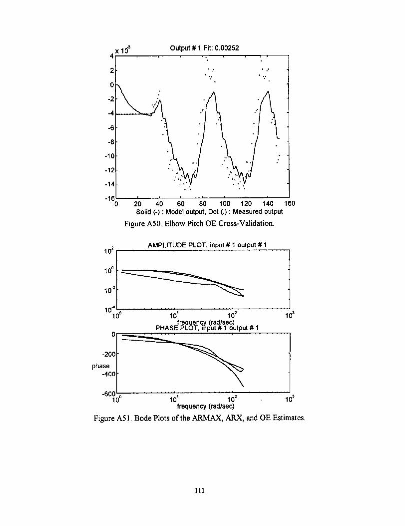
x 1034
2
0
-2
-4
-6
-8
-10
-12
-14
-160
Output # 1 Fit: 0.00252
= = i • , I = i • =
• _ • •
• *.* 16
.',
I I I I I | I
20 40 60 80 100 120 140
Solid (-) : Model output, Dot (.) : Measured output
Figure A50. Elbow Pitch OE Cross-Validation.
%_°" •
• ° ,
• •
6O
102AMPLITUDE PLOT, input # 1 output # 1
,oo 10 .2
10_,0o .................. 101 102
frequency (rad/sec)PHASE PLOT, input # 1 output # 1
103
Pha ot-60100o .................. 101 102 103
frequency (racl/sec)
Figure A51. Bode Plots of the ARMAX, ARX, and OE Estimates.
lll
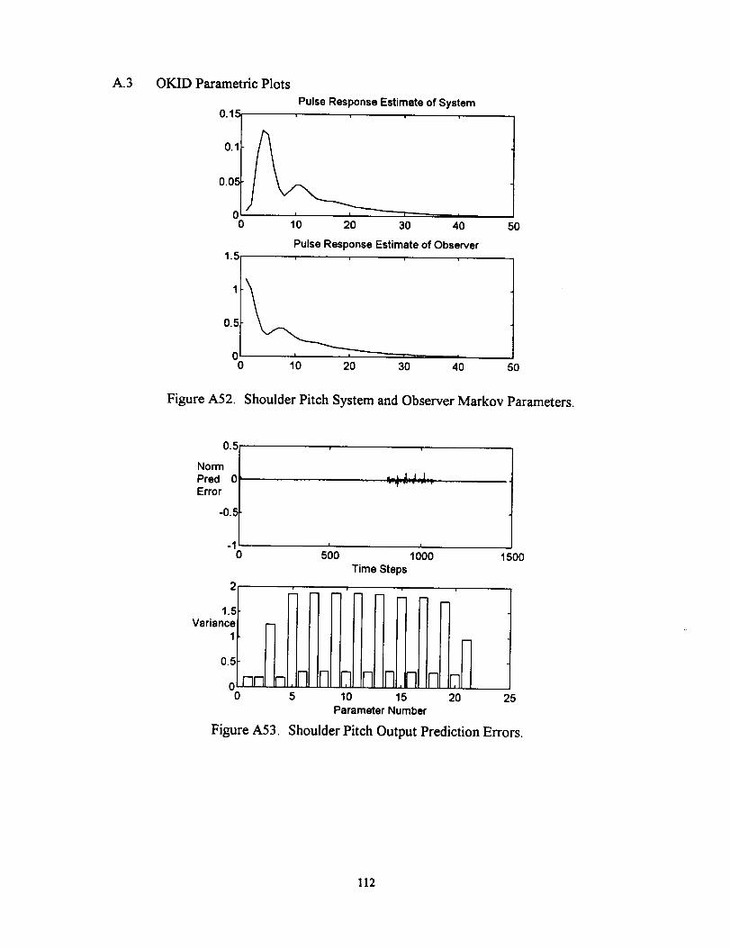
A.3 OKID Parametric Plots
0.1_=
0.1 //_
°,°_/ \0'
0
1.5
Pulse Response Estimate of System
1_0 20 30 40
Pulse Response Estimate of Observer
50
0.5
\!
0 10 20 30 40 50
Figure A52. Shoulder Pitch System and Observer Markov Parameters.
0.5
NormPred 0 'Error
-0.I
-10
,._L_ I. JJ._
I !
500 1000 1500Time Steps
1.5Variance
1
0.5
00
i
Nm
5
Figure A53.
nilnlnnl10 15
Parameter Number
Shoulder Pitch Output Prediction Errors.
r
20 25
112

Hankel Matrix Singular Values101
10o
Mag
10 -1
10.2
10-3
10-4
10s , , , ,0 2 4 6 8
Number
Figure A54. Shoulder Pitch Hankel Matrix.
10
0
Mag.(db)
-20
Response due to input= 1 output= 1
-.40 ........ i ........ l ........ i .......
lO.2 lO" loo lO' ldFrequency (Hz)
0
Angle
(Deg)
-20C
-40C ..................................10.2 10"I 100 101 102
Frequency (Hz)
Figure A55. Shoulder Pitch Bode Plots of State-Space Estimate
113
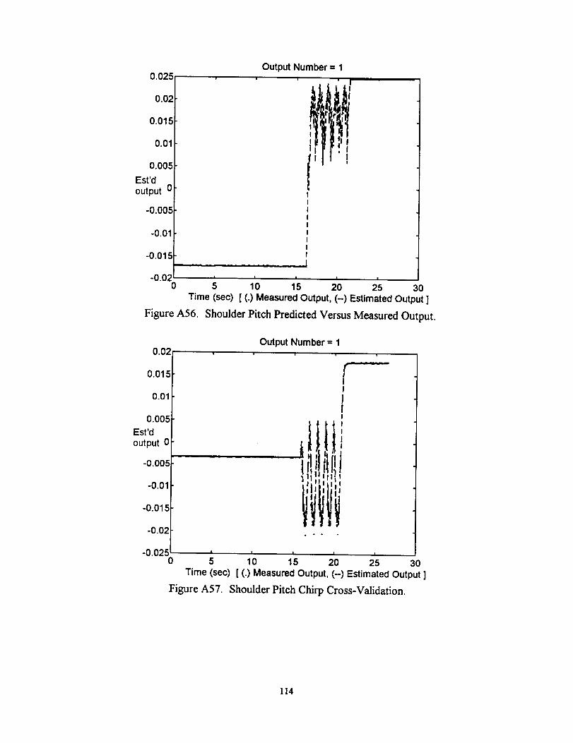
0.025
0.02
0.015
0.01
0.005
Est'doutput 0
-0.005
-0.01
-0.015
-0.020
Figure A56.
Output Number = 1
!
.............. ..]
I I I I I
5 10 15 20 25 30Time (sec)[ (.) Measured Output, (--) Estimated Output ]
Shoulder Pitch Predicted Versus Measured Output.
0.02
0.015
0.0"
0.005
Esrdoutput 0
-0.005
-0.01
-0.015
-0.02
-0.0250 5
Time (sec)
Figure A57.
Output Number = 1
ltfti
I I I I
10 15 20 25 30
[ (.) Measured Output, (-) Estimated Output ]
Shoulder Pitch Chirp Cross-Validation.
114
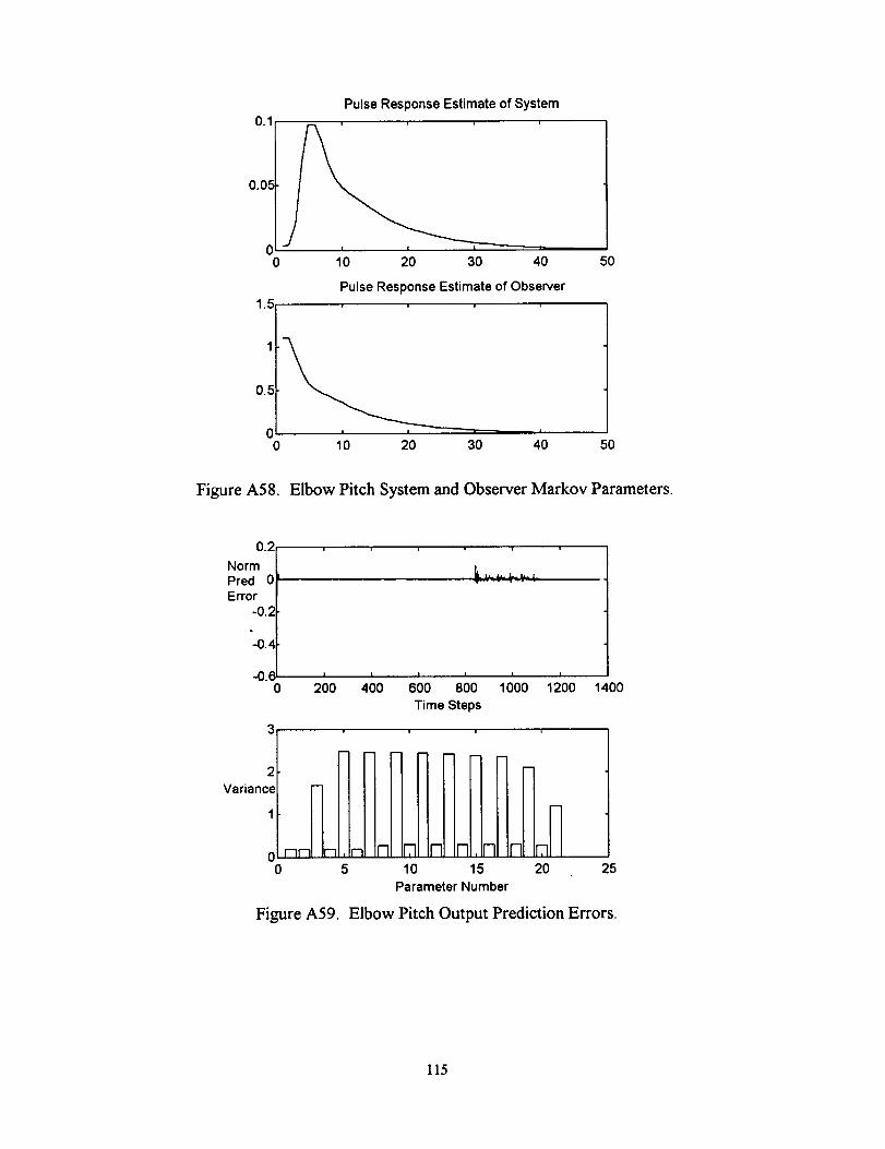
0.1Pulse Response Estimate of System
0.05 I
00 10 20 30 40 50
1.5
0.5
Pulse Response Estimate of Observer
0 , _ '0 10 20 30 40 50
Figure A58. Elbow Pitch System and Observer Markov Parameters.
0.2
NormPred 0Error
-0.2
"-0.4
I
-0.6 ' ' ' ' ' I0 200 400 600 800 1000 1200 1400
Time Steps
Vrancit0nnH nnnrain0 5 10
i
15 20
Figure A59.
25
Parameter Number
Elbow Pitch Output Prediction Errors.
115
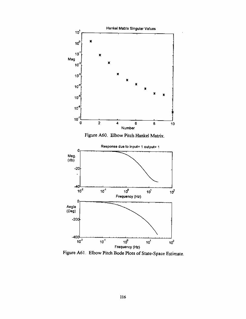
101
loo
10-1
Mag
10;
lo"
lo"
lo"
10.70
0
Mag.(db)
-20
--4O10.2
0
Angle(Deg)
-20(
-40(10.2
Figure A61.
Hankel Matrix Singular Values
i
I I I I
2 4 6 8Number
Figure A60. Elbow Pitch Hankel Matrix.
10
Response due to input= 1 output= 1
....... f ......
I .... ...t , .,,I
lo-1 lo0 lo1 lo_Frequency (Hz)
i .......
lo_ loo _o' lo_Frequency (Hz)
Elbow Pitch Bode Plots of State-Space Estimate.
116
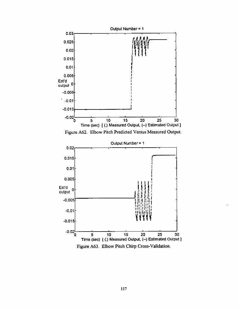
0.03Output Number = 1
0.025
0.02
0.015
0.01
0.005Est'doutput 0
-0.005
-0.015
Jtti
!!IIIIIiII
-0.020 5 10 15 20 25 30
Time (sec) [ (.) Measured Output, (-) Estimated Output ]
Figure A62. Elbow Pitch Predicted Versus Measured Output.
0.02Output Number = 1
0.015
0.01
0.005
Est'd0
output
-0.005
-0.01
-0.01
-0.020
Figure A63.
r--]!
!I
]I
Ili
II:!
1 '!f
t I1 _1! 1' J_ IIlll I1111]
I I I I I
5 10 15 20 25 30Time (sec) [ (.) Measured Output, (-) Estimated Output ]
Elbow Pitch Chirp Cross-Validation.
117
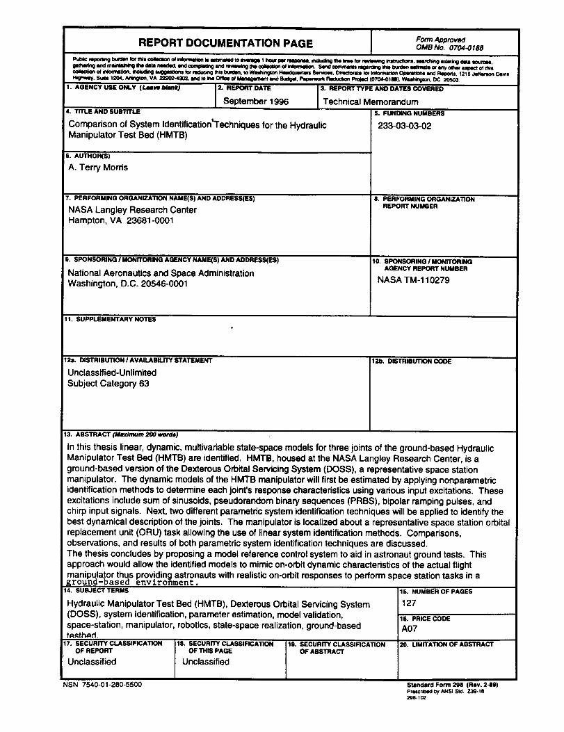
REPORT DOCUMENTATION PAGE FormApprovedOM8 No. 0704-0188
Put_ mpom'.g burr_n tOt b_'s ool_cSk_ of WJomW._ Is ew_m_ lo ewn_e 1 hour por rmm_le, mctuctmg me wne tor _ _n.cY_ns. Imarct,ng ommg qJala _.
gathertng mtd ma_lRJC_g the data mmfWJ. Imd (_mP)xt_r.o and m'4mmg the oM_c_n o_ _me_n. Ser.d oommer_ reoamtng _ bur_n el_P4te or eny oC_er mq_cl ol _
ceCoctiono/inloeeetlon,include0_ggestlen= fermduemgthinI_,rmn. to WmC_in_eeHNdmjjmn _. Omx:tomm_ _ _ _ _m. 121SJelfer_e Daw=H_hwly. Sule 1204. Arl_. VA 2220Q-4_lndlol_neOfficeof Mln_andBuCl_l. PI_ Reductmn Pro_ (0704.O188),WIMW_. _ 20503,
1. AGENCY USE ONLY (L_ve b/am/r) 2. HF.PORT DATE 3. REPORT TYPE AND DATES COVERED
September 1996 Technical Memorandum4. TITLE AND SUb(i'H.E S. FUNDING NUMBERS
Comparison of System Identification_echniques for the Hydraulic 233-03-03-02Manipulator Test Bed (HMTB)
s. AUTHOR(S)
A. Terry Morris
7. PERFORMINGORGANIZATIONNAME(S)ANDADDRESS(ES)
NASA Langley Research CenterHampton, VA 23681-0001
9. SPONSORINGI MONiTOHINGAGENCYNAME(S)ANDADDRESS(ES)
National Aeronautics and Space Administration
Washington, D.C. 20546-0001
8. PERFORMING ORGANIZATIONREPORT NUMBER
10. SPONSORING/MONITORINGAGENCY REPORT NUMBER
NASA TM-110279
11. SUPPLEMENTARY Nq_rl_5
12a. DiS_IBUTION I AVAILABILITY STATEMENT
Unclassified-Unlimited
Subject Category 63
12b. DISTRIBUTION CODE
13. ABSTRACT (Maximum 200 won_)
In this thesis linear, dynamic, multivariable state-space models for three joints of the ground-based HydraulicManipulator Test Bed (HMTB) are identified. HMTB, housed at the NASA Langley Research Center, is aground-based version of the Dexterous Orbital Servicing System (DOSS), a representative space station
manipulator. The dynamic models of the HMTB manipulator will first be estimated by applying nonparametricidentification methods to determine each joint's response characteristics using various input excitations. These
excitations include sum of sinusoids, pseudorandom binary sequences (PRBS), bipolar ramping pulses, andchirp input signals. Next, two different parametric system identification techniques will be applied to identify the
best dynamical description of the joints. The manipulator is localized about a representative space station orbitalreplacement unit (ORU) task allowing the use of linear system identification methods. Comparisons,observations, and results of both parametric system identification techniques are discussed.
The thesis concludes by proposing a model reference control system to aid in astronaut ground tests. This
approach would allow the identified models to mimic on-orbit dynamic characteristics of the actual flightmanipulator thus providing astronauts with realistic on-orbit responses to perform space station tasks in a_round-based environment.
14. SUBJECT TERMS
Hydraulic Manipulator Test Bed (HMTB), Dexterous Orbital Servicing System(DOSS), system identification, parameter estimation, model validation,
space-station, manipulator, robotics, state-space realization, ground-basedtn._thnd
17. SECURITY CLASSlRCATION 18. SECURITY CLASSlRCATION 19, SECURITY CLASSIFICATIONOF REPORT OF THIS PAGE OF ABSTRACT
Unclassified Unclassified
NSN 7540-01-280-5500
15. NUMBER OF PAGES
127
16. PRICE CODE
A07
20. UMITATION OF ABSTRACT
Standard Form 298 (Rev. 2-89)PruCnI_Kl by ANSI Sld Z39-18
298-1C_