comparison of simulated annealing, genetic, and tabu...

Iranian Journal of Oil & Gas Science and Technology, Vol. 4 (2015), No. 2, pp. 50-67 http://ijogst.put.ac.ir

Comparison of Simulated Annealing, Genetic, and Tabu Search Algorithms for Fracture Network Modeling

Saeed Mahmoodpour, Mohsen Masihi*, and Sajjad Gholinejhad

Department of Chemical and Petroleum Engineering, Sharif University of Technology, Tehran, Iran

Received: February 23, 2014; revised: December 08, 2014; accepted: December 20, 2014

Abstract

The mathematical modeling of fracture networks is critical for the exploration and development of natural resources. Fractures can help the production of petroleum, water, and geothermal energy. They also greatly influence the drainage and production of methane gas from coal beds. Orientation and spatial distribution of fractures in rocks are important factors in controlling fluid flow. The objective function recently developed by Masihi et al. 2007 was used herein to generate fracture models that incorporate field observations. To extend this method, simulated annealing, genetic, and tabu search algorithms were employed in the modeling of fracture networks. The effectiveness of each algorithm was compared and the applicability of the methodology was assessed through a case study. It is concluded that the fracture model generated by simulated annealing is better compared to those generated by genetic and tabu search algorithms.

Keywords: Spatial Configuration of Fractures, Simulated Annealing, Genetic Algorithm, Tabu Search Algorithm, Fracture Network

1. Introduction

There are three main reasons for a detailed study and modeling of naturally fractured reservoirs:

1. To site best locations for production wells; 2. To study the response of natural fractures under simulation pressure, and hence to develop

best scenario for hydraulic fracture treatment; 3. To design an optimum production method and evaluate reservoir potential.

In order to achieve the prescribed objectives, naturally fractured reservoirs need to be characterized and modeled (Tran et al., 2003; Masihi et al., 2007). Stochastic reservoir models must honor as much data as possible to turn into reliable numerical models of the studied reservoir (Clayton et al., 1994). Researchers have attempted to model natural fractures with idealized approaches such as the sugar cube and the slab models. Classical geo-statistical methods often fail to predict the distribution of the fractures. Recent trends in reservoir characterization tend to use more sophisticated tools such as global optimization methods (Ouenes et al., 1994; El Ouahed et al., 2003 Tran et al., 2003; Masihi et al., 2007; Tran et al., 2007; Shekhar et al., 2008). There are many methods currently used to solve a large spectrum of problems. However, simulated annealing, genetic, and tabu search algorithms are becoming the standard approaches. For engineers and scientists eager to reach a certain global

* Corresponding Author:

Email: [email protected]

S. Mahmoodpour / Comparison of Simulated Annealing, Genetic, and Tabu Search … 51

optimum or to match some fields or experimental data, these methods are very useful (Ouenes et al., 1994). Masihi et al. 2007 proposed an objective function based on the fracturing process for fracture network modeling. Shekhar et al. 2011 used this objective function for the generation of spatially correlated fracture models through simulated annealing algorithm for seismic simulations and described the periodic boundary condition implementation in this method. Masihi et al. 2012 extended this methodology to fracture network modeling in a three dimensional plane (Shekhar et al., 2011; Masihi et al., 2012). We follow Masihi et al. (2007) and use simulated annealing, genetic, and tabu search algorithms to generate fracture models. These are stochastic optimization methods that have been used in different kinds of problems that involve finding global optimum values of a function consisting of a large number of independent variables. The efficiency of each algorithm was compared with others, and the applicability of the methodology was assessed through a case study.

2. Basic concepts

2.1. Objective function

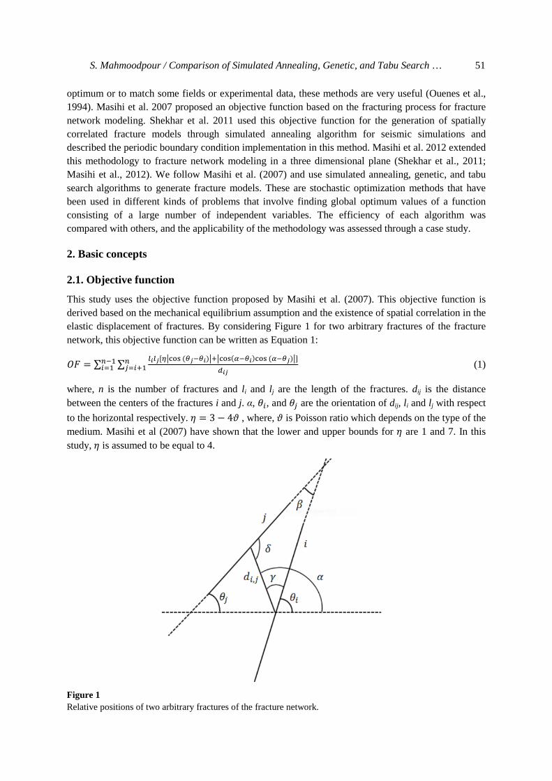
This study uses the objective function proposed by Masihi et al. (2007). This objective function is derived based on the mechanical equilibrium assumption and the existence of spatial correlation in the elastic displacement of fractures. By considering Figure 1 for two arbitrary fractures of the fracture network, this objective function can be written as Equation 1:

�� ∑ ∑ �� (1)

where, n is the number of fractures and l i and l j are the length of the fractures. dij is the distance between the centers of the fractures i and j. α, ��, and �� are the orientation of dij, l i and l j with respect

to the horizontal respectively. � � 3 � 4! , where, ! is Poisson ratio which depends on the type of the medium. Masihi et al (2007) have shown that the lower and upper bounds for � are 1 and 7. In this study, � is assumed to be equal to 4.

Figure 1 Relative positions of two arbitrary fractures of the fracture network.

52 Iranian Journal of Oil & Gas Science and Technology, Vol. 4 (2015), No. 2

This objective function has the capability of being updated during calculations rather than being re-computed for each new perturbation. Except for the first iteration, it is only needed to compute the change in the objective function between the consecutive perturbations instead of re-calculating the objective function itself.

2.2. Perturbation mechanism

For generating a new fracture configuration based on the current one, a mechanism to effect a small random change is needed. In this study, the mentioned randomly selected small change is called fracture i. The selected fracture, as an individual object, experiences one or some of the following possible changes:

Grow or shrink (increasing or reducing its size): "��#$ � "� % 0.5�2* � 1� (2)

Rotate (changing its orientation):

��#$ � �� % 0.05 , �2* � 1� (3)

Shift (changing its position): -��#$ � -� % 0.5 �2* � 1� (4)

.��#$ � .� % 0.5 �2* � 1� (5)

where, R is a random number selected from a uniform distribution in the range of [0-1].

3. Description of various techniques employed in the study

3.1. Simulated annealing

Metropolis has developed the idea of numerically simulating molecular behavior (Metropolis et al., 1953). From concepts developed in thermodynamics, it is known that a system will change from a state of energy Ei to another state of energy Ej with the below probability:

/�∆E� � exp �5�� 5�67 8 � (6)

where, T denotes the temperature of the heat bath and KB is a physical constant known as the Boltzmann constant. The system will always change if Ej is less than Ei. However, sometimes an unfavorable step may take place. The application of this probability distribution in the numerical simulation of systems composed of several parts has come to be known as the Metropolis algorithm. Kirkpatrik (Kirkpatrick et al., 1983) and independently Cerny (Cerny 1982) extended these concepts to combinatorial optimization. They formulated an analogy between the objective function and the free energy of a thermodynamic system. A control parameter, analogous to temperature, is used to control the iterative optimization algorithm until a state with a low objective function (energy) is reached.

The general algorithm may be described by the following steps:

1. Generate an initial image; 2. Establish an initial control parameter T and schedule for lowering it as the looping progresses;


3. Perturb the image; 4. Compute a new objective function (OF new); 5. Establish the acceptance probability distribution:

P:accept> � ? 1 if ��#$ B ��C��exp��C�� #$D �, otherwiseK (7)

6. Draw from that probability distribution; if the perturbation is accepted, then update the image and reset the objective function. OF�NO � OFPQR;

7. Return to step 3 until a step criterion is reached.

3.2. Genetic algorithm (GA)

The basic principles of GA were introduced by Holland (Holland 1975). A GA is a search method based on natural selection and genetics. The main theme of the research on GA has been the robustness and the balance between the efficiency and the efficacy necessary for survival in many different environments. GA is computationally simple, yet powerful, and is not limited by assumptions about the search space (Jeong 1996). Unlike many other optimization techniques, GA uses a pool of solutions. This is known as a population which appeals to the biological analogy. New models are then constructed from this pool by applying various genetic operations. The basic GA uses three operations known as reproduction, cross-over, and mutation. The reproduction operator is a stochastic operator, which selects models from current population in such a way that better models are more likely to be selected. Crossover operates on the models previously selected by reproduction and combines them together to form new models. Mutation is a random perturbation, which is applied to the newly generated models. These newly generated models form current population and this generation process is repeated until the termination criterion is satisfied (Xavier et al., 2013; Khansary et al., 2014; Toledo et al., 2014).

The general algorithm may be described with the following steps:

1. Generate some random solutions (current population); 2. Calculate quality of solutions and rank these solutions according their qualities; 3. Choose two solutions from population according to their qualities for reproduction; 4. Check the reproduction probability; if satisfactory, produce two new solutions from the

current ones by the cross-over operator; 5. Check mutation probability; if satisfactory, perturb the newly generated solution; 6. Two of these four solutions return to the population according to their qualities; 7. Return to step 3 until a stop criterion is reached.

3.3. Tabu search

The word tabu comes from Tongan, a language of Polynesia, where it was used by the aborigines of Tonga Island to indicate things which cannot be touched because they are sacred. Fred Glover proposed a new approach, which he called tabu search, to allow hill climbing to overcome local optima (Glover 1989). Tabu search is a deterministic method, which uses repeated local searches, avoids entrapment in local minima, and encourages the exploration of unreached regions. Tabu search achieves this through the storage of information relating to the previous models sampled. These historical records are referred to as tabu lists. In practice, several tabu lists can be maintained containing information such as models previously visited or previously accepted improving moves. Under some circumstances, the tabu conditions can be ignored when a criterion known as the


aspiration condition is satisfied. Such conditions are included to allow interesting moves, which would otherwise be rejected (Unver et al., 2011; Prot et al., 2012; Hussin et al., 2014).

The general algorithm may be described with the following steps:

1. Generate an initial image; 2. Generate some solutions by perturbing mechanism and put these moves in the tabu list; 3. Generate neighboring solutions around the best solution in the list; 4. Find the best neighboring solution; 5. Check accessibility; if satisfied, accept it and replace the current solution and update the tabu

list; if not, select the second best neighboring solution; 6. Return to step 3 until a stop criterion is reached.

4. Case study

We compare the capacity of TS, GA, and SA algorithms in fracture network modeling by studying the fault map of Otsego county and the surrounding area (New York, USA) as shown in Figures 2 and 3 (Tran et al., 2003). There were 442 fractures in the target network. One of the major limitations in the discrete fracture network modeling is to populate fracture data in large DFN models. It is emphasized that the fracture data obtained either from 1-D well data or scan-line data introduce significant errors in the produced models. In the case study of the current work, conventional field studies (cores, image logs, seismic measurements, outcrop, production data, drilling data, etc.) provided data for some fracture orientation, length, and position. They were assigned as conditional data and were exempted from the perturbation mechanism. The fracture network was modeled using SA, GA, and TS. Each model will be discussed individually below.

Figure 2 Fault map of Otsego county and surrounding area (New York, USA).


Figure 3 Digitization of Figure 2; known data are colored blue and the data which should be simulated are colored red.

Simulated annealing: initial images were first generated randomly. If the initial value of the temperature T is chosen too high, too many bad uphill moves will be accepted. On the other hand, if the initial value of T is chosen too low, the algorithm will then drop into a local minimum. For the 100 iterations before the main program run, the value of the objective function was calculated. It is assumed that the objective function variations have a normal distribution, and thus:

STTUVW *XWYZ � [Z. Z\ XTTUVWU] ^Z_U`[Z. Z\ VaZVZ`U] ^Z_U` b 1 b exp :� c|∆��|eeeeeeee % 3f∆ghiDj >

(8)

where, |∆��|eeeeeeee is the absolute average value of the difference in the objective function and f∆gh stands for the standard deviation of this normal distribution. Equation 9 leads to the rule for the computation of the initial temperature as reads:

Dj � exp k� c|∆��|eeeeeeee % 3f∆ghi1S* l (9)

The described perturbation mechanism was employed for generating new images of the fracture network. In the most general simulated annealing algorithm (homogeneous Markov chains), the temperature remains constant through NT iterations, and it is then reduced and kept constant for the next NT iterations. These NT iterations represent one Markov chain. We applied this method and used NT=100 for the inner loop. The simplest and most commonly used schedule for T updating is geometrical schedule that is expressed by the Equation 10. This schedule was used with m � 0.97:

D�#$ � m DC�� (10)

Fracture density (m/m2) was assumed as a stop criterion.

0 10 20 30 40 50 60 70 80 90 1000

10

20

30

40

50

60


To eliminate the effects of finite boundaries, appropriate periodic boundary conditions (PBC) should be selected. However, there are some limitations as this would lead to an infinite number of pairs of fractures. For choosing an appropriate limit for the PBC, the approach of Shekhar et al. (2011) was employed. This is by establishing a criterion for determining the maximum distance, which leads to the number of repeated model cells. The minimum number of periodic images required for an appropriate PBC can be calculated as follows:

if rcut-off > a, then N= rcut-off /a, else N= (rcut-off /a) +1.

where, a is the average of the length and width of the representative model and N representing the largest integer value, is the model images required for the PBC. The number of periodic images surrounding the original model will be equal to N in the x- and y-directions to neutralize the effect of boundaries of the model cell. The PBC can be implemented by copying enough images of the model to extend to a distance of rcut-off in all directions. In this study, the original model includes 1500 fractures in a rectangular area (100 by 60 km), each fracture is about 2 km in length with a random orientation between -30 and +30 (Figure 4). During simulating annealing and to evaluate the change in the fracture configuration, the objective function (Equation 11) is required, which has the important parameters such as the relative orientation of the fractures and the ratio of the length of fractures. This is also used to find the cut-off radius. For detailed analysis, an arbitrary fracture (the first fracture of the test model) was taken and the total initial energy was calculated by Equation 11:

�� p S"�"��cosc�� iq�r�� % cos�m � �� cos �m � ��/a��

(11)

Figure 4 The starting model used for testing the parameters affecting periodic boundary condition implementations; this model consists of 1500 fractures in a rectangular area with a length of 100 km and a width of 60 km.

The effect of orientation and the relative length of other fractures were quantified by re-computing the total energy value while rotating a single fracture, changing a single fracture length at (x, y) = (1, 4), (1, 6), (1, 8), (1, 12), (1, 16), (1, 20), and (1, 24) one at a time, or changing the orientation by 15 degree (Figures 5 and 6). The results confirm that fractures close to the reference fracture have

0 10 20 30 40 50 60 70 80 90 1000

10

20

30

40

50

60


significantly more influence than fractures at a distance. This is not surprising given that energy is inversely proportional to distance (Equation 11). In fact, fractures at distances larger than 20 km have negligible influence on the total energy value. Therefore, for the present modeling study, the cut-off radius, which is the distance up to where fractures influence each other, is 20 km. The results of simulation are presented in Figures 7 and 8. To evaluate the effect of considering the PBC, the simple statistical measures in the results of SA were compared with and without PBC in Table 1.

Figure 5 The effect of rotation (relative orientation) of a fracture on total energy value; r is the y coordinate of the test fracture that is rotated; the x coordinate of the test fracture was 1 km.

Figure 6 The effect of relative fracture lengths on total energy value; Li is the first fracture and Lj is the fracture the length of which is changed.

394

395

396

397

398

399

400

401

402

403

0 50 100 150 200

OF

Rotation angle (degrees)

r2

r4

r6

r8

r12

r16

r20

r24

390

395

400

405

410

415

420

425

430

435

0 2 4 6 8 10

OF

L j/ L i

r2

r4

r6

r8

r12

r16

r20

r24


As seen in Figure 7, an overall network area of 300 km (length) by 180 km (width) was used herein and the network area of our interest, with a length of 100 km and a width of 60 km, is located in the center of the overall network. In fact, nine networks with the same dimensions were used as the previously mentioned area of interest and known data were assigned to all of them. While changing the configuration of fractures by perturbing their position, some fractures close to the boundary were removed from the model, and thereby affecting the number density of fractures in the model.

Figure 7 Illustration of the produced fracture network for the implementation of PBC that contains a representative fracture network at its center; the representative fracture network at the center is surrounded by eight similar fracture networks with the same size.

Figure 8 Interested fracture network with the implementation of PBC.

0 50 100 150 200 250 3000

20

40

60

80

100

120

140

160

180

100 110 120 130 140 150 160 170 180 190 20060

70

80

90

100

110

120


Table 1 Comparison of the statistics of SA simulation results with and without PBC.

Statistical measurement

SA SA with PBC

Mean-x 47.92 48.85

Standard deviation-x 27.06 27.32

Kurtosis-x -1.15 -1.19

Skewness-x 0.06 0.04

Mean-y 30.12 30.53

Standard deviation-y 16.28 16.34

Kurtosis-y -1.19 -1.31

Skewness-y 0.09 -0.02

Mean-l 9.70 9.68

Standard deviation -l 9.78 9.14

Kurtosis-l 6.97 9.73

Skewness-l 2.10 2.28

Mean-θ 82.42 84.12

Standard deviation-θ 52.95 51.96

Skewness-θ 0.22 0.28

Kurtosis-θ -1.34 -1.18

Figure 9 Fracture network image generated from the simulated annealing algorithm simulation.

In addition to applying PBC, one can only use the area of interest and discard the perturbations which cause artifact problems and perturb the fractures again. The generated network by this method is shown in Figure 9. Hence, the PBC was implemented in SA algorithm and the obtained results were close to those obtained without using the PBC. The comparison of Figure 8 and Figure 9 shows that

0 10 20 30 40 50 60 70 80 90 1000

10

20

30

40

50

60


one may use this simple method, while the result is good enough and the run time is much shorter than that used in the PBC. Since the run time of the implementation of PBC is in agreement with the simple method (i.e. discarding the bad perturbations), and because the results are reasonable and the ultimate goal is to generate just a realization of the fracture network, the SA with the simple method of discarding the bad perturbations was used in this study.

It should be noted that one of main disadvantages of the SA method is the high computational requirement. Although, faster variants of the SA exist, they are not quite easily coded and hence are not widely used. There are some adaptive SA versions which could be used for solving this problem (Laarhoven et al., 1987; Lam et al., 1988; Triki et al., 2005). However, the adaptation of these adaptive versions to our problem is beyond the scope of this study.

Genetic algorithm: 50 images of the fracture network were first generated randomly as a solution population and ranked according to their qualities. Two of them were randomly chosen for reproduction and probability with respect to their qualities. Values of 0.8 and 0.05 were used for cross-over and mutation probabilities respectively; in other words, a number from the normal distribution was taken. If the chosen number is less than 0.8, cross-over occurs, and if this number is less than 0.05, mutation happens. Two of these four solutions (two chosen and two produced) are returned to the population according to their qualities and the new population is generated. Similar to the simulated annealing, fracture density is used as a stop criterion.

Tabu search: the image was first generated randomly. By a perturbation mechanism, 50 new images were generated and the fracture number at which perturbation occurred was entered on the tabu list. The best solution from the tabu list was chosen and five new solutions were generated from it. As described before, the algorithm continued until it reached the stop criterion (fracture density).

5. Results and discussion

The GA, SA, and TS algorithms described above were implemented using MATLAB programming on a personal computer with a core i5, 2.67 GHz CPU. The fracture networks resulted from SA, GA, and TS are shown in Figures 9-11 respectively.

Figure 10 Fracture network image generated from the genetic algorithm simulation.

0 10 20 30 40 50 60 70 80 90 1000

10

20

30

40

50

60


Contour maps were used to demonstrate the distribution of the fracture center point locations (Figures 12 through 15). Histograms with an interval length of 2 were used to demonstrate the fractures length distribution (Figure 16), and histograms with an interval length of 5 were used for fracture orientation comparison (Figure 17). To make a better comparison, simple statistical measurements, shown in Table 2, were used for the simulation results and the actual data.

Figure 11 Fracture network image generated from the tabu search algorithm simulation.

Figure 12 Contour map of fracture center point locations for the real data.

0 10 20 30 40 50 60 70 80 90 1000

10

20

30

40

50

60

0.875

0.87

5

0.8750.875 0.875

0.8750.875

0.87

5

0.875

0.87

5

0.87

5

0.87

50.

875

0.875

0.87

5

0.875

0.87

5

0.875

0.875

0.875

0.87

50.

875

1.75

1.75

1.75

1.75

1.75

1.75

1.75

1.75

1.75

1.75

1.75 1.75

1.75 1.75

1.75

1.75

1.75

1.75

1.75 1.75

1.75

1.75

1.75

1.75

1.75

1.75

1.75

1.75

1.75

1.75

1.75

2.62

5 2.625

2.625

2.62

5

2.625

2.6252.625

2.625

2.625

2.625

2.62

5

2.625

2.625

2.62

52.625

2.625

2.625

2.625

2.62

5

2.625

2.625

3.5 3.5

3.5

3.5

3.5

3.5

3.53.5

3.53.5 3.

5

3.5

3.5

3.53.5


Figure 13 Contour map of fracture center point locations for the simulated annealing algorithm simulation result.

Figure 14 Contour map of fracture center point locations for the genetic algorithm simulation result.

0.750.75

0.750.75

0.75

0.75

0.75 0.75

0.75

0.75

0.75

0.75

0.75

0.75

0.75

0.75

0 .750.75

0.75

0.75

1.5

1.5 1 .5

1.5

1.51.5

1.5

1.5

1.5

1.5

1.5

1.5

1.5

1.5

1.5

1.5

1.5

1.5

1.5

1.5

1.5

1.5

1.5

1.5

1.5

1.5

1.5

1.5

1.51.5

1.5

2.252.

25

2.25

2.252.25

2.25

2.25

2.252.25

2.25

2.25

2.25

2.25

2.25

2.25

2.25

2.25

2.25

2.25

2.25

2.25

2.25

2.25

2.252.25

2.252.25

2 .252.25

2.25

3 3

3

33

3

33

33

3

3

3

33

3

3

3

3

333

3

3

33

3

33.753.75

3.753.75

3.75

3.753 .

75

4.5

4.5

4.5

4.5

4.5

0.75

0.75

0.750.75 0.

75

0.75

0.75

0.750.75

0.75

0.75

0.75

0.75

0.75

0.75

0.75

0.75

0.75

1.5

1.5

1.5

1.5

1.5

1.5

1.5

1.5

1.5

1.5

1.5

1.5

1.5

1.5

1.5

1.51.

5

1.5

1.5

1.5

1.5

1.5

1.5

1.5

1.5

1.5

1.51.

5

1.5

1.52.

25

2.25

2.25

2.25

2.25

2.25

2.25

2.25

2.25

2.25

2.25

2.25 2.25

2.25

2.25

2.25

2.25

2.25

2.25

2.25

2.252.25 2.252.25

2 .25

2.25

2.25

2.25

2.25

3

3

3

33

3

3

3

3

33

3

33

3

3 3

3

3

3

3

3

3

3

3

33

3.75

3.75

3.75

3.75

3.75

3.75

3.75

3.75

3 .75

3.75

3.75

4.5

4.5


Figure 15 Contour map of fracture center point locations for the tabu search algorithm simulation result.

Figure 16 Histogram of fracture length distribution.

1

1

1

1

1

1

1

1

1 1 1

1

1

1

1

1

1

1

1

1

1

11

1

1

1

1

2

2

2

2 2 2

2

2

2

2

2

2

2

2

2

2

2

2

2 2 22

2

22

2

22

2

2

2

2

2

2

2

2

3

3

3

33

3 33

33

33

3

33

3

33

3

33

3

33

4

44

4

4

44

44

4

4

4

5

5

5

55

566

6

7

0

20

40

60

80

100

120

0 20 40 60 80 100

Fra

ctur

es a

boun

dnes

s

Fractures length interval

genetic

real

annealing

tabu


Figure 17 Histogram of fracture orientation distribution.

Table 2 Comparison of the simulation results and the real data in simple statistical measurements.

Statistical measurement Real SA GA TS

Mean-x 47.24 47.92 49.46 48.36

Standard deviation-x 29.08 27.06 28.21 27.26

Kurtosis-x -1.16 -1.15 -1.20 -1.15

Skewness-x 0.15 0.06 0.05 0.03

Mean-y 31.05 30.12 30.20 30.35

Standard deviation-y 18.02 16.28 16.36 16.13

Kurtosis-y -1.26 -1.19 -1.22 -1.18

Skewness-y -0.05 0.09 -0.03 0.04

Mean-l 9.71 9.70 9.68 9.70

Standard deviation-l 8.56 9.78 8.92 10.22

Kurtosis-l 11.67 6.97 9.70 6.07

Skewness-l 2.59 2.10 2.30 2.03

Mean-θ 77.76 82.42 85.07 83.75

Standard deviation-θ 50.94 52.95 54.58 53.67

Skewness-θ 0.39 0.22 0.19 0.17

Kurtosis-θ -1.07 -1.34 -1.32 -1.35

0

5

10

15

20

25

30

35

40

0 50 100 150 200

Fra

ctur

es a

boun

dnes

s

Fractures orientation interval

genetic

real

annealing

tabu


6. Conclusions

The objective function of Masihi et al. (2007) was followed and simulated annealing, genetic algorithm, and tabu search algorithm were used to generate fracture network models. The capability of TS, GA, and SA algorithms in fracture network modeling was compared by studying the fault map of Otsego and the surrounding area. The fracture models were generated using SA, GA, and TS algorithms. The detailed comparison of the simulation results and the real data showed that the simulated annealing had the best results but its run time (269 s) was greater than those of GA (242 s) and TS (195 s). The qualities of the SA results are much better than those of the other algorithms. Moreover, the SA with the simple method (i.e. discarding the bad perturbations) is preferred to the method of using PBC, since the results are reasonable, the run time is significantly lower, and the ultimate goal is to generate the realizations of the fracture network.

Nomenclatures

AR : Accept ratio

GA : Genetic algorithm

SA : Simulated annealing

TS : Tabu search

OF : Objective function

d : Distance between fracture centers

E : Energy

KB : Boltzmann constant

l : Fracture length

n : Number of fractures

NT : Markov chain length |∆��|eeeeeeee : Absolute average value of the difference in objective function

R : Random number from normal distribution

T : Temperature

α : Orientation of d with respect to the horizontal

η : Constant number depends on rock type

θ : Orientation of fracture with respect to the horizontal

ν : Poisson ratio

σOF : Standard deviation of objective function difference distribution

i : Fracture i

j : Fracture j

References

Cerny, V., A Thermodynamical Approach to the Traveling Salesman Problem: An Efficient Simulation Algorithm, Journal of Optimization Theory and Application, Vol. 45, p. 41-51, 1985.

Clayton, V. D and Andre, G., The Application of Simulated Annealing to Stochastic Reservoir Modeling, SPE Adv. Technology, Ser. Vol. 2, No. 2, p. 222-227, 1994.


El Ouahed, A. K., Tiab, D., Mazouzi, A., and Sarfraz, A., Application of Artificial Intelligence to Characterize Naturally Fractured Reservoirs, SPE International Improved Oil Recovery Conference in Asia Pacific, Kuala Lumpur, Malaysia, 20-21 October, 2003.

Golver, F., Tabu Search, ORSA Journal on Computing, Vol. 1, p. 190-206, 1989. Holland, J., Adaptation in Natural and Artificial Systems: An Introductory Analysis with Application

to Biology, Control, and Artificial Intelligence, the University of Michigan Press, 1975. Hussin, M. S. and Stutzle, T., Tabu Search vs. Simulated Annealing as a Function of the Size of

Quadratic Assignment Problem Instances, Computers & Operations Research, Vol. 43, p. 286-291, 2014.

Jeong, I. L. K., Adaptive Simulated Annealing Genetic Algorithm for System Identification, Engng Applic. Artif. Intell, Vol. 9, No. 5, p. 523-532, 1996.

Khansary, M. A. and Sani, A. H., Using Genetic (GA) and Particle Swarm Optimization (PSO) Methods for Determination of Interaction Parameters in Multicomponent Systems of Liquid-Liquid Equilibria, Fluid Phase Equilibria, Vol. 365, p. 141-145, 2014.

Kirkpatrick, S., Gellat, C.D., and Vechhi, M. P., Optimization by Simulated Annealing, Science, Vol. 220, p. 671-680, 1983.

Laarhoven, P. J. M. V. and Aaarts, E. H. L., Simulated Annealing: Theory and Application, Kluwer Academic Publishers, 1987.

Lam, J. and Delosme, J. M., Performance of a New Annealing Schedule, 25th ACM/IEEE Design Automation Conference, New York, 1988.

Masihi, M. and King, P., Connectivity of Spatially Correlated Fractures: Simulation and Field Studies, paper SPE 107132 presented at the SPE Europe/EAGE Annual Conference and Exhibition, London , United Kingdom, 11-14 June, 2007.

Masihi, M., Sobhani, M., Al-Ajmi, A. M., Al-Wahaibi, Y. M., and Al-Wahaibi, T. K., A Physically-based Three Dimensional Fracture Network Modeling Technique, Scientia Iranica, Vol. 19, No. 3, p. 594-604, 2012.

Metropolis, N., Rosenbluth, A., Rosenbluth, M., Teller, A., and Teller, E., Equation of State Calculations by Fast Computing Machines, Journal Chem. Phys., Vol. 21, No. 6, p. 1087-1092, 1953.

Ouenes, A. and Bhagavan, S., Application of Simulated Annealing and Other Global Optimization Methods to Reservoir Description(Myths and Realities), SPE Annual Technical Conference and Exhibition, New Orleans, Louisiana, 25-28 September, 1994.

Prot, D. and Morineau, O.B., Tabu Search and Lower Bound for an Industrial Complex Shop Scheduling Problem, Computers & Industrial Engineering, Vol. 62, p. 1109-1118, 2012.

Shekhar, R., Ricard, L., and Gibson, A., Correlated Fracture Network Modeling Using Simulated Annealing, SEG Annual Meeting, Las Vegas, Nevada, 2008.

Shekhar, R., Richard, L., and Gibson, A., Generation of Spatially Correlated Fracture Models for Seismic Simulations, International Geophysical Journal, Vol. 185, p. 341-351, 2011.

Toledo, C. F. M., Oliveira, L., and Franca, P. M., Global Optimization Using a Genetic Algorithm with Hierarchically Structured Population, Journal of Computational and Applied Mathematics, Vol. 261, p. 341-351, 2014.

Tran, N. H., Chen, Z., and Rahman, S. S., Object-based Global Optimization in Modeling Discrete-Fracture Network Map: A Case Study, SPE Annual Technical Conference and Exhibition, 5-8 October, Denver, Colorado, 2003.


Tran, N. H. and Tran, K., Combination of Fuzzy Ranking and Simulated Annealing to Improve Discrete Fracture Inversion, Elsevier, Mathematical and Computer Modeling, Vol. 45, p. 1010-1020, 2007.

Triki, E., Collette, Y., and Siarry, P., A Theoretical Study on the Behavior of Simulated Annealing Leading to a New Cooling Schedule, European Journal of Operational Research, Vol. 166, No. 1, p. 77-92, 2005.

Unver, N. F. and Kokar, M. M., Self-controlling Tabu Search Algorithm for the Quadratic Assignment Problem, Computers & Industrial Engineering, Vol. 60, p. 310-319, 2011.

Xavier, C. R., Santos, E. P. D., Vieira, V. D. F., and Santos, R. W. D., Genetic Algorithm for the History Matching Problem, Procedia Computer Science, Vol. 18, p. 946-955, 2013.

comparison of simulated annealing, genetic, and tabu...

Documents