comparison of different statistical downscaling methods to estimate changes in hourly extreme...

INTERNATIONAL JOURNAL OF CLIMATOLOGYInt. J. Climatol. (2014)Published online in Wiley Online Library(wileyonlinelibrary.com) DOI: 10.1002/joc.4138

Comparison of different statistical downscaling methodsto estimate changes in hourly extreme precipitation using

RCM projections from ENSEMBLES

Maria Antonia Sunyer,a* Ida Bülow Gregersen,a Dan Rosbjerg,a Henrik Madsen,b

Jakob Luchnerb and Karsten Arnbjerg-Nielsena

a Department of Environmental Engineering, Technical University of Denmark, Kongens Lyngby, Denmarkb DHI, Hørsholm, Denmark

ABSTRACT: Changes in extreme precipitation are expected to be one of the most important impacts of climate change incities. Urban floods are mainly caused by short duration extreme events. Hence, robust information on changes in extremeprecipitation at high-temporal resolution is required for the design of climate change adaptation measures. However, thequantification of these changes is challenging and subject to numerous uncertainties.

This study assesses the changes and uncertainties in extreme precipitation at hourly scale over Denmark. It exploresthree statistical downscaling approaches: a delta change method for extreme events, a weather generator combined with adisaggregation method and a climate analogue method. All three methods rely on different assumptions and use differentoutputs from the regional climate models (RCMs). The results of the three methods point towards an increase in extremeprecipitation but the magnitude of the change varies depending on the RCM used and the spatial location. In general, a similarmean change is obtained for the three methods. This adds confidence in the results as each method uses different informationfrom the RCMs. The results of this study highlight the need of using a range of statistical downscaling methods as well asRCMs to assess changes in extreme precipitation.

KEY WORDS climate change; extreme; precipitation; high-temporal resolution; RCM; statistical downscaling

Received 2 April 2014; Revised 15 July 2014; Accepted 23 July 2014

1. Introduction

Both the intensity and frequency of extreme precipita-tion events are expected to increase in Northern Europe(Christensen and Christensen, 2003; Lenderink and vanMeijgaard, 2008; Seneviratne et al., 2012). This increaseis likely to be one of the most relevant impacts of cli-mate change in cities (Fowler and Hennessy, 1995). Hence,information on these changes and their associated uncer-tainty is crucial for the design and adaptation of urbaninfrastructure such as drainage systems.

Several studies assess the changes in extreme precipita-tion under future climate conditions (e.g. Frei et al., 2006;Grum et al., 2006; Gregersen et al., 2013). In these studies,regional climate model (RCM) outputs are the most com-monly used primary source of information. RCMs pro-vide precipitation projections at a higher spatial resolution(often at approximately 25 km) than global climate models(GCMs) (often at 100 km or more). For this reason, RCMsare considered more adequate to represent extreme precip-itation at the regional scale than GCMs. In recent years,relatively large multimodel ensembles of RCMs have been

* Correspondence to: M. A. Sunyer, Department of EnvironmentalEngineering, Technical University of Denmark, Miljøvej building 113,Kongens Lyngby 2800, Denmark. E-mail: [email protected]

made freely available, e.g. the RCMs from the ENSEM-BLES project (van der Linden and Mitchell, 2009) forEurope and the RCMs from NARCCAP (Mearns et al.,2013), which cover North America. These ensembles pro-vide information to estimate projections of precipitationextremes and make an assessment of the associated uncer-tainty. While outputs from RCMs are commonly availableat daily scale, only few models have readily available out-put at sub-daily and hourly scale. RCM simulations athourly scale are more computer demanding in terms ofpre- and post-processing needs, and their performance athourly scale is often considered worse than at daily scale(e.g. Hanel and Buishand, 2010; Gregersen et al., 2013).

In addition, it is generally accepted that RCMs aresubject to two main drawbacks: they inherit the biasesfrom GCMs and their spatial resolution is too large forassessing extreme precipitation impacts at the local spatialscale. Therefore, statistical downscaling of RCM outputsis needed to obtain high spatial resolution, bias-correctedextreme precipitation projections. Several methods havebeen suggested and used in the literature, including deltachange approaches (e.g. Sunyer et al., 2012), generalizedlinear models using atmospheric variables as covariates(e.g. Maraun et al., 2011), weather generators (WGs) (e.g.Burton et al., 2008) and resampling based methods (e.g.Willems and Vrac, 2011). However, only a few methods

© 2014 Royal Meteorological Society

M. A. SUNYER et al.

have been applied at sub-daily precipitation scales (e.g.Onof and Arnbjerg-Nielsen, 2009; Willems and Vrac,2011; Olsson et al., 2012).

The quantification of changes in extreme precipitationunder future climate conditions is intrinsically challeng-ing and subject to numerous uncertainties. The lack ofRCMs available at sub-daily scale makes the assessmentof changes at these temporal scales even more challenging.This is critical because it is at the sub-daily scale at whichextreme precipitation causes the largest urban floods.

This study investigates the expected changes and uncer-tainties in extreme precipitation at hourly scale overDenmark. It explores three statistical downscaling meth-ods: a delta change method for extreme events, a WG com-bined with a disaggregation method and a climate analoguemethod. All three methods rely on different assumptionsand use different outputs from the RCMs. The aim ofthis study is to compare the changes estimated from thethree statistical downscaling methods applied to an ensem-ble of RCMs over Denmark. These changes are analysedbased on their dependence on return period, RCM and spa-tial location. The results from this study are part of theinformation used to provide guidelines for urban drainagedesign in Denmark.

The next section introduces the data used. Section 3describes the methodology, and Section 4 presents anddiscusses the results followed by the conclusions.

2. Data

This section describes the observational data sets andRCMs used in the study. The three statistical downscal-ing methods require both different observations and differ-ent RCM outputs. The delta change method does not useobservational data to estimate the changes in extreme pre-cipitation, whereas the other two methods use both griddedand point observations. The gridded observations used arethe Danish data set Climate Grid Denmark (CGD) (Schar-ling, 2012) and the European data set E-OBS (Hofstraet al., 2009). Daily precipitation data from CGD is basedon approximately 300 stations covering Denmark and hasa spatial resolution of 10× 10 km2 (Figure 1). The timeperiod available for this data set is 1989–2010. E-OBS isa gridded daily data set based on the pan-European sta-tion network ECA&D (Klein Tank et al., 2002). It coversthe time period 1951–2012 and has a spatial resolution of0.22 degrees (approximately 25 km).

Station data is used to obtain information of sub-dailyprecipitation properties. Four stations from the DanishSVK data set are used in the disaggregation method.This data set consists of approximately 100 stations with1-min resolution precipitation records for the time period1979–2012 (Jørgensen et al., 1998; Thomsen, 2013). Thefour stations chosen for this study have been selectedto represent low and high extreme precipitation indicesand to be well distributed over Denmark (see locations inFigure 1). In the climate analogue method data from a setof high-temporal resolution stations over Europe has been

CGD

SVK

1 h max.

1 h max. and 1 h

(a)

1

2

3

4

(b)

Figure 1. (a) Grid points in CGD and selected SVK stations, and (b) gridpoints of the different RCMs used in this study. In (b) the black circlesrepresent the common grid points to all RCMs, and the stars are the extra

grid points used from the ensemble of 13 RCMs.

analysed, see K. Arnbjerg-Nielsen et al., pers. comm. formore details.

All the climate models used in this study are RCMs fromthe ENSEMBLES project (van der Linden and Mitchell,2009). An ensemble of 13 RCMs with a spatial resolutionof 0.22 degrees and a temporal resolution of 1 day hasbeen used (Table 1). Results from these RCMs also containinformation on the daily 1-h maximum precipitation. Inaddition, two of the ENSEMBLES’ RCMs have beenmade available at 1-h resolution, HIRHAM5-ECHAM5and RACMO2-ECHAM5. The time period covered bythe RCMs is 1950–2100. The time periods consideredfrom the RCMs are 1961–1990 and 2071–2100, whichare selected to represent present and future conditions,respectively.

The selected spatial domain for the RCMs is all the landgrid points over Denmark. In the 13 models at daily timestep, the land grid points are defined as grid points with a

© 2014 Royal Meteorological Society Int. J. Climatol. (2014)

STATISTICAL DOWNSCALING METHODS FOR EXTREME PRECIPITATION

Table 1. List of RCMs used in this study, driving GCMs andsource of the RCMs.

Number RCM GCM Institute

1 HIRHAM5 ARPEGE DanishMeteorologicalInstitute

2 HIRHAM5 ECHAM53 HIRHAM5 BCM4 REMO ECHAM5 Max Planck Institute

for Meteorology5 RACMO2 ECHAM5 Royal Netherlands

MeteorologicalInstitute

6 RCA ECHAM5 SwedishMeteorological andHydrological Institute

7 RCA BCM8 RCA HadCM3Q39 CLM HadCM3Q0 Swiss Federal Institute

of Technology, Zürich10 HadRM3Q0 HadCM3Q0 UK Met Office11 HadRM3Q3 HadCM3Q312 HadRM3Q16 HadCM3Q1613 RCA3 HadCM3Q13 Community Climate

Change Consortiumfor Ireland

land/water fraction above 0.4 combined with a subjectivecomparison with the coastline of Denmark. The grid pointsused for the two models at 1-h resolution are the sameas the ones used in Gregersen et al. (2013). These wereselected as the grid points with a land/water fraction above0.5. There is a difference of six grid points between the twocriteria, which is not expected to affect the results. Figure 1shows the grid points used for each of the data sets.

3. Methodology

This section describes the three statistical downscalingmethods applied in the study. All three methods are basedon a change factor methodology (Sunyer et al., 2012), i.e.they use RCM outputs to estimate relative change (abso-lute change in the case of mean temperature) from presentto future of one or several climate variable properties (e.g.change in mean precipitation). These changes, referred toas change factors or climate factors (CFs), are then appliedto the local spatial scale. The use of CFs assumes thatfor the selected properties the same factors are valid atthe large and the local spatial scale. It also assumes thatthe RCMs can represent the change in precipitation prop-erties better than the magnitude of precipitation. Variousstudies have addressed the ability of the RCMs in rep-resenting extreme precipitation. These studies show thatthe RCMs present biases in short duration extreme precip-itation, which is mainly caused by convective precipita-tion (e.g. Hanel and Buishand 2010; Kendon et al., 2012;Gregersen et al., 2013). The bias in convective precipita-tion is expected to arise mainly from the spatial resolu-tion and the convective precipitation scheme used in the

RCMs (Kendon et al., 2012). It also implicitly assumesthat the bias in the RCM properties will remain constantfrom present to future. It should be noted that this assump-tion might not be valid, Sunyer et al. (in press) show thatthe precipitation bias of the RCMs depends on the precip-itation value and that this might change in the future.

3.1. Delta change of extreme precipitation

This method assumes that the changes in extreme precip-itation estimated from the large spatial scale of the RCMsalso represent the changes at the local scale. This statisticaldownscaling approach is applied to the daily 1-h maxi-mum precipitation and to the daily precipitation outputsfrom the RCMs. The approach is divided in two parts: firstthe extreme events for each grid point in the RCMs forpresent and future are estimated for different return peri-ods T; and then the CFs of these events are calculated as theratio between the two estimates. The values of T consid-ered here are 2, 10 and 100 years. It must be noted that theonly output of this method is the changes in extreme pre-cipitation at the local scale. This method does not generatetime series for the future time period at the local scale.

The first step to estimate the T-year events is to extractthe extreme value series from the time series. This is doneusing a partial duration series (PDS) methodology, wherean average of three events per year is applied to select theextreme value series. An independence criterion based onthe inter-event time between extremes is used to ensurethat only independent events are included in the extremevalue series. Here, only events separated by more than 1day are considered. The T-year events are estimated byfitting a Generalized Pareto Distribution (GPD) using aregional estimated shape parameter, following the regionalL-moment approach by Hosking and Wallis (1993). Thisapproach assumes that the shape parameter is homogenousover the region as shown by Madsen et al. (2002). Oncethe T-year events have been estimated from the RCMs,CFs are calculated for each value of T and for each gridpoint. The results of this method are referred to as DC inthe results section.

In order to assess the influence of using daily 1-h maxi-mum precipitation from the RCMs, the same approach hasalso been applied to the 1-h precipitation series availablefor two of the RCMs. The extreme precipitation simulatedby these two RCMs was studied in detail by Gregersenet al. (2013). The same PDS method is used to extractthe extreme value series from the hourly RCMs, using aslightly different independence criterion as described byGregersen et al. (2013). The use of different independencecriteria is not expected to affect the results. The resultsobtained using the two RCMs at hourly resolution arereferred to as DC-1h in the results section.

3.2. Weather generator and disaggregation

This approach is based on two separate steps: (1) firstdaily time series are generated using a WG; (2) then thesedaily time series are disaggregated into high-temporalresolution time series. The WG is calibrated separately for


M. A. SUNYER et al.

each grid point in CGD using the CGD data and changesin precipitation properties from the RCM outputs. It isapplied to generate daily time series for present and futureconditions. The disaggregation model is calibrated usingthe SVK point observations. It is applied to the generateddaily time series to obtain 30 min temporal resolutiontime series for each grid point in CGD for present andfuture conditions. A temporal resolution of 30 min ischosen because it is close to the resolution needed inurban drainage design. It is also chosen because the samescaling properties of precipitation are valid for temporalresolutions ranging from approximately 30 min to 1 day.Nguyen et al. (2007) showed that there is a shift in thescaling properties of precipitation at a temporal resolutionof approximately 40 min. This section describes first theWG and then the disaggregation model.

The WG used in this study is the Neyman-ScottRectangular Pulses (NSRP) (Cowpertwait et al., 1996)implemented in the RainSim software (Kilsby et al., 2007;Burton et al., 2008). This WG is based on a clusteringapproach, whereby precipitation is represented as clustersof rain cells that form storm events. Storm events in NSRPare defined through four steps (Kilsby et al., 2007): (1)a storm origin arrives following a Poisson process, (2) aPoisson process is used to generate a random number ofrain cells, which are separated from the storm origin byexponentially distributed time intervals, (3) the durationand intensity of each cell are estimated using exponentialdistributions and (4) for each time step, the intensities ofall the active cells are summed to obtain the total intensity.In the single-site application, five parameters are neededto describe the NSRP model. The parameters are fittedfor each month separately using precipitation properties.In RainSim, a large number of properties can be used.In this study we use: daily mean precipitation, variance,skewness and probability of dry day. RainSim allows theuse of different weights for each statistic. Here we selecta weight of 6, 2, 4 and 4 for the mean, variance, skewnessand probability of dry day, respectively. These weightsare considered suitable for the representation of bothmean and extreme precipitation (a relatively high weightis assigned to the skewness). It should be noted that inRainSim the weights do not need to sum up to 1 (Burtonet al., 2008).

For the present period, the observed properties fromCGD are used to fit the NSRP model for each grid pointand generate 100 years long synthetic time series of dailyprecipitation. The properties of precipitation for the futureperiod is found by calculating monthly CFs as the ratiobetween the estimates for future and present time periodsfrom the RCMs for each grid point. The CFs are then usedto perturb the precipitation properties of the CGD gridpoints to obtain the expected values for the future periodusing the approach described by Sunyer et al. (2012).Nearest neighbour interpolation is used to obtain the CFsat the spatial resolution of CGD. As in the present period,the values for the future period are used to fit the WG foreach grid point and generate 100 years long synthetic timeseries of daily precipitation.

In the second step of this statistical downscalingapproach, the synthetic time series are disaggregated intotime series with a temporal resolution of 30 min. Thisis done using the canonical cascade model described byMolnar and Burlando (2005). This model uses a cascadegenerator to distribute precipitation intensity on two suc-cessive regular subdivisions of an interval. The cascadegenerator is composed of an intermittency factor, whichdivides the domain into rainy and non-rainy fractions, anda factor which defines the rain intensity. The parametersof the cascade generator are estimated from the temporalscaling properties of the sample moments of the SVKstations. The parameters are estimated separately foreach season and for the four SVK stations. The seasonsconsidered are: winter (December to February), spring(March to May), summer (June to August) and autumn(September to November). The same notation as inMolnar and Burlando (2005) is used here to describe thesteps followed to estimate the parameters of the cascadegenerator.

For each station and season, the scaling propertiesare analysed using seven levels, n, where n equal to 0and 6 correspond to 32 and 0.5 h, respectively. As themodel considers two regular subdivisions, the temporalresolutions analysed here are: 0.5, 1, 2, 4, 8, 16, and32 h. The last level considered is 32 h to ensure that theproperties at 24 h are included in the analysis. The tem-poral resolution in the cascade model is expressed usingthe scale, 𝜆n, which is defined as 2−n, where 2 refers tothe number of subdivisions in the cascade model. Thenon-central moments, Mn(q), of order q for 0< q< 4 arethen estimated for each 𝜆n. A log–log linear regressionis fitted for each q relating Mn(q) and 𝜆n. The negativevalue of the slope of this linear regression is 𝜏(q). TheMandelbrot-Kahane-Peyriere function is then fitted to thevalues of 𝜏 to estimate the two parameters of the cascadegenerator, 𝛽 and 𝜎2, which are related to the intermittencyand variability of the cascade generator, respectively.

Once the disaggregation model has been calibratedusing the SVK data, it is applied to each of the daily timeseries generated with the WG. It must be noted that whendisaggregating from 24 h into two successive regular sub-divisions, the final temporal resolution is 22.5 min. As inOnof and Arnbjerg-Nielsen (2009), linear interpolation isused to obtain the time series at 30 min, i.e. four intensitiesat 22.5 min are interpolated to obtain three intensities at30 min.

It must be noted that this approach is based on theassumption that the temporal scaling properties of pre-cipitation used in the disaggregator are constant frompresent to future. It also assumes that the precipitationproperties used in the WG are valid to represent extremeprecipitation both in the present and future. This approachis referred to as WGD-24h in the results section, the24h notation is used to indicate that only RCM prop-erties at 24 h are used. T-year events and their CFs areestimated from the time series generated for the presentand future using the same PDS methodology describedfor DC.



3.3. Climate analogue

This method is based on using a set of known vari-ables (predictors) to identify a region where the presentconditions resemble the future conditions of the regionbeing studied. The method has been applied within climatechange and other disciplines (e.g. Hallegatte et al., 2007;Bennion et al., 2011; Arnbjerg-Nielsen, 2012).

A set of indices are used as predictors, i.e. monthly meanand standard deviation of daily temperature, monthly meanand standard deviation of daily precipitation, monthly pro-portion of dry days, and 1- and a 10-year event of dailyprecipitation. These indices are estimated for the futureperiod in Denmark in two steps. First, each index is esti-mated for each grid point in E-OBS covering Denmarkand then they are averaged to obtain a single value rep-resenting the region. The index for the future is estimatedby perturbing the value for the present period using CFs.These are calculated from the RCMs as the average overall the RCMs and grid points covering Denmark. Indicesfor present conditions are estimated for all the grid pointsin Europe using E-OBS.

From the six indices, an aggregate metric is definedthat measures the similarity between future indices inDenmark and present indices in Europe. For each gridpoint, the metric is calculated as the weighted average ofthe difference between the indices at the grid point andthe indices for the future period in Denmark. A weightof 0.22 is given to mean temperature, mean precipitationand extreme precipitation, whereas a weight of 0.11 isgiven to the proportion of dry days, standard deviation oftemperature and precipitation.

The region with the lowest metric is selected to representthe climate in Denmark under future conditions. Historicalrecords of precipitation extremes from a set of locations inthis region are then collected. T-year events for hourly datafrom these locations are used to represent future extremeprecipitation in Denmark. CFs are estimated as the ratiobetween these T-year events and the T-year events forpresent conditions in Denmark.

As the other two methods, this approach also relies onseveral assumptions. It assumes that an analogue regionfor extreme precipitation exists and that it can be repre-sented by the indices chosen. This approach is referred toas CA-24h in the results section. For more details on thismethod and its application see K. Arnbjerg-Nielsen et al.,pers. comm. As in WGD-24h, the 24h notation is used toindicate that only RCM properties at 24 h are used in thismethod.

4. Results and discussion

The results presented in this section are divided in twosubsections. First, the results from each statistical down-scaling method are discussed. Then, the CFs of the T-yearevents obtained from each method are compared. Thiscomparison is divided in three parts. The first part presentsthe overall results at hourly and daily scale and focuses onthe main differences and similarities between the methods.

0.8 1 1.2 1.4 1.6 1.8

(a)

(c)

(b)

(d)

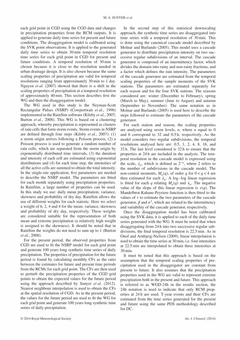
Figure 2. CF estimated at each grid point in DC (panels (a) and (c))and DC-1h (panels (b) and (d)) for the 2-year return period forHIRHAM5-ECHAM5 (panels (a) and (b)) and RACMO2-ECHAM5(panels (c) and (d)). The reader is referred to the online version of this

article for the correct visualization of the colours used in this figure.

The second and third parts focus on the variation ofthe hourly CFs within the RCMs and within the region,respectively.

4.1. Statistical downscaling methods

4.1.1. Delta change of extreme precipitation

The influence of using daily 1-h maximum precipitationto estimate changes in hourly extreme precipitation isassessed by comparing the results of DC and DC-1h.Differences may arise from the way in which maximumhourly precipitation is obtained. For example, it couldbe that the daily 1-h maximum precipitation is chosenusing a moving average window of 1-h as opposedto the hourly data with consecutive hourly precipita-tion amounts. Figure 2 shows the CFs obtained for the2-year return period from the two approaches using theRCM–GCM combinations: HIRHAM5-ECHAM5 andRACMO2-ECHAM5. The 2-year return period is selectedbecause the spatial pattern is clearer than for the 10- and100-year return period.

The magnitude and spatial pattern obtained from thetwo methods using HIRHAM5-ECHAM5 are quite sim-ilar. The regional sample means are 1.44 for DC and1.41 for DC-1h and the regional sample standard devia-tions are 0.07 for DC and 0.06 for DC-1h. In the case ofRACMO2-ECHAM5, the results of the two methods areslightly more different than for HIRHAM5-ECHAM5. Forthis model, the results for DC-1h include both decreasesand increases of extreme precipitation, whereas the resultsof DC point to an increase of extreme precipitation inall grid points. Additionally, the difference between theregional averages is slightly larger (1.19 and 1.14 for DC


M. A. SUNYER et al.

−2 −1.5 −1 −0.5 0

0

0.5

1

1.5

2

2.5

3

3.5

log(λ)

log

(M(q

))

0 1 2 3 4

−1.5

−1

−0.5

0

0.5

q

τ(q

)

Winter

Summer

q=1

q=2

q=3

(a) (b)

Figure 3. (a) Log–log relation between non-central moments and temporal scale, values of log(𝜆) equal to 0 and −1.8 correspond to 32 and 0.5 h,respectively. (b) Negative slope of the log–log linear regressions. The results shown in (a) and (b) are for the station 4 (see location in Figure 1).

and DC-1h, respectively). The regional standard devia-tions are similar for the two methods (0.12 and 0.14 forDC and DC-1h, respectively). For both RCMs, a largerregional average is found for DC when compared toDC-1h.

This brief comparison shows that the use of daily 1-hmaximum precipitation or hourly time series has a smallimpact on the results. The reasons for these differencesare out of scope of this study and will not be analysedfurther. Here the daily 1-h maximum precipitation outputsare used because they are available for all 13 RCMs. Thisallows us to assess the variation of CF within the RCMs.Nonetheless, it must be kept in mind that the CFs obtainedusing DC might be slightly larger than the CFs that wouldbe obtained using DC-1h if all the RCMs were available athourly resolution.

4.1.2. Weather generator and disaggregation

Multiple studies have evaluated the ability of the NSRPWG to represent observed precipitation properties (suchas mean, variance, skewness, autocorrelation and proba-bility of dry days) as well as extreme value series (Burtonet al., 2008, 2010; Cowpertwait, 1998; Cowpertwait et al.,1996). These studies conclude that NSRP WG can satis-factorily represent the main precipitation properties andextreme events at the daily scale in climates similar to theregion studied here. Therefore, this section focuses on theresults from the disaggregation approach.

Figure 3 shows the precipitation properties used in thedisaggregation approach for winter and summer period forone of the SVK stations. In both seasons, the momentsshow the expected linear relationship (Figure 3(a)). Theslope of the linear regressions differs from winter to sum-mer. For moments of order higher than 1 the slope issmaller in the summer period, i.e. in summer the differ-ence between the precipitation events of short and longdurations is smaller than in winter. The difference betweenthe two seasons is higher for higher order moments(Figure 3(b)). The smaller slopes for high order momentsfound for the summer period illustrate the importance ofshort duration extreme events in this season, which aremainly caused by convective precipitation.

The ability of the canonical cascade to represent extremeprecipitation at high-temporal resolution is evaluated usingthe SVK data. Each station has been disaggregated usingtwo different set of parameters: the parameters found forthat station, and the average of the parameters found forall the stations. For each case, the canonical cascade hasbeen run 10 times to illustrate the variability in the results.Figure 4 shows the extreme value series at hourly resolu-tion from the observed and the disaggregated time seriesusing the two sets of parameters. Overall, the disaggre-gated time series reproduce the observed extreme eventssatisfactorily, although they tend to slightly underestimatehigh extremes. The use of different parameters for eachstation does not improve the results significantly. For thisreason and for simplicity, the average of the parametersfound for all the stations is used to disaggregate the dailytime series generated using the WG.

4.1.3. Climate analogue

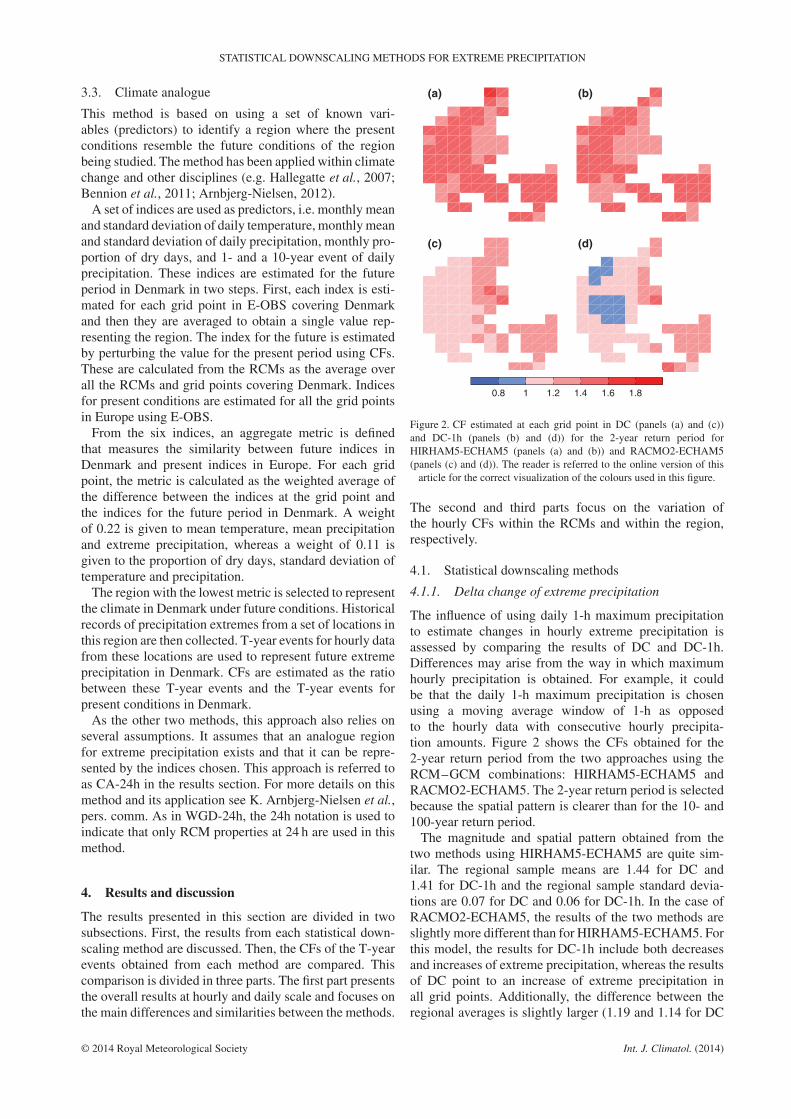
Figure 5 shows the metric estimated with the climateanalogue method together with the stations available inthe regions of interest. These are the regions where themetric is close to 0, i.e. higher similarity to the futureclimate in Denmark. The most relevant regions are thenorthwest of France, Belgium, The Netherlands, westcoast of Denmark and southeast of Britain. The lowestvalue of the metric is found in the northwest of France,from where extreme precipitation information is availablefor five stations at high-temporal resolution. Data fromthese stations are only available in processed form, i.e.for return periods between 1 and 10 years and durationsbetween 10 min and 6 h. As only five stations are includedin the analysis, the variance of the CFs is not reported forthis downscaling method. See K. Arnbjerg-Nielsen et al.,pers. comm. for more results of this method.

4.2. Changes in extreme precipitation

4.2.1. Overall results and variation within methods

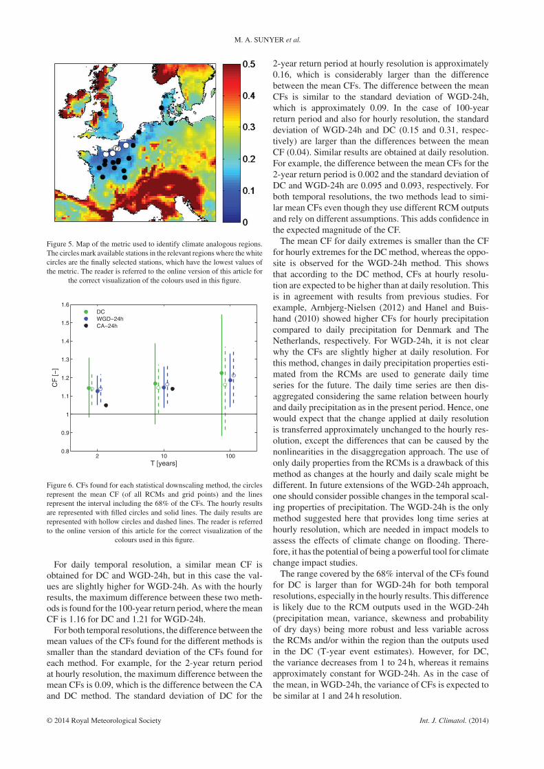
Figure 6 shows the mean CF for 2-, 10- and 100-year returnperiod for each statistical downscaling method for 1 and24 h temporal resolution. The figure also shows the range



100

101

0

5

10

15

20

25

30

[mm

h–1]

100

101

0

5

10

15

20

25

30

100

101

0

5

10

15

20

25

30

[mm

h–1]

T [years]10

010

10

5

10

15

20

25

30

T [years]

Disagg. TS − Same param.

Disagg. TS − Diff. param.

Observed TS

Station 1 Station 2

Station 3 Station 4

Figure 4. Extreme values at hourly resolution estimated from the observations and ten disaggregated time series using two sets of parameter: theaverage parameters of all the station (+) and the individual parameters for each station (o).

covered by the 16th and 84th empirical percentiles. Thesepercentiles are estimated from the sample containing allthe CFs of all grid points and RCMs. The range coveredby these empirical percentiles is denoted as the 68% inter-val, which corresponds to a 68% confidence interval ignor-ing the interdependency arising from correlation betweenRCMs (Sunyer et al. 2013) and spatial dependence. Asthese assumptions are questionable, the true confidencebounds for the CFs are likely to be higher than shown inthe figure. It must be noted that the natural variability is notexplicitly addressed in the results shown in this section.Nonetheless, it is undoubtedly present in the interval ofCFs shown in Figure 6.

In general, there is good agreement between the threemethods. Some differences are observed between themethods depending on the temporal resolution of the CFsand return period, but overall they are not significant.The mean CF of all methods points towards an increaseof extreme precipitation (CF> 1) for both 1 and 24 h. Inmost cases, the lower confidence bound is also higher

than 1. It is lower than 1 for DC for all return peri-ods of the hourly extremes, and for daily extremes for areturn period of 100 years. As expected, for all the meth-ods the mean as well as the range covered by the 68%interval of the CFs increase for higher return periods.The increase in the range covered by the 68% interval ofthe CFs is to some extend affected by the higher naturalvariability and sampling uncertainty in the higher returnperiods.

For the hourly temporal resolution and the 2-year returnperiod, the mean CFs obtained for DC and WGD-24hare virtually equal, 1.14 and 1.13, respectively. How-ever, the mean CF for CA-24h is slightly lower, approx-imately 1.05. For the 10-year return period the meanCF of the three methods is similar, the values rangebetween 1.14 for CA-24h to 1.17 for DC. A similar resultis found for the 100-year return period, the mean CFfound is 1.19 for WGD-24h and 1.23 for DC. For allthe return periods the mean CF in DC is higher than inWGD-24h.


M. A. SUNYER et al.

Figure 5. Map of the metric used to identify climate analogous regions.The circles mark available stations in the relevant regions where the whitecircles are the finally selected stations, which have the lowest values ofthe metric. The reader is referred to the online version of this article for

the correct visualization of the colours used in this figure.

2 10 1000.8

0.9

1

1.1

1.2

1.3

1.4

1.5

1.6

T [years]

CF

[−

]

DC

WGD−24h

CA−24h

Figure 6. CFs found for each statistical downscaling method, the circlesrepresent the mean CF (of all RCMs and grid points) and the linesrepresent the interval including the 68% of the CFs. The hourly resultsare represented with filled circles and solid lines. The daily results arerepresented with hollow circles and dashed lines. The reader is referredto the online version of this article for the correct visualization of the

colours used in this figure.

For daily temporal resolution, a similar mean CF isobtained for DC and WGD-24h, but in this case the val-ues are slightly higher for WGD-24h. As with the hourlyresults, the maximum difference between these two meth-ods is found for the 100-year return period, where the meanCF is 1.16 for DC and 1.21 for WGD-24h.

For both temporal resolutions, the difference between themean values of the CFs found for the different methods issmaller than the standard deviation of the CFs found foreach method. For example, for the 2-year return periodat hourly resolution, the maximum difference between themean CFs is 0.09, which is the difference between the CAand DC method. The standard deviation of DC for the

2-year return period at hourly resolution is approximately0.16, which is considerably larger than the differencebetween the mean CFs. The difference between the meanCFs is similar to the standard deviation of WGD-24h,which is approximately 0.09. In the case of 100-yearreturn period and also for hourly resolution, the standarddeviation of WGD-24h and DC (0.15 and 0.31, respec-tively) are larger than the differences between the meanCF (0.04). Similar results are obtained at daily resolution.For example, the difference between the mean CFs for the2-year return period is 0.002 and the standard deviation ofDC and WGD-24h are 0.095 and 0.093, respectively. Forboth temporal resolutions, the two methods lead to simi-lar mean CFs even though they use different RCM outputsand rely on different assumptions. This adds confidence inthe expected magnitude of the CF.

The mean CF for daily extremes is smaller than the CFfor hourly extremes for the DC method, whereas the oppo-site is observed for the WGD-24h method. This showsthat according to the DC method, CFs at hourly resolu-tion are expected to be higher than at daily resolution. Thisis in agreement with results from previous studies. Forexample, Arnbjerg-Nielsen (2012) and Hanel and Buis-hand (2010) showed higher CFs for hourly precipitationcompared to daily precipitation for Denmark and TheNetherlands, respectively. For WGD-24h, it is not clearwhy the CFs are slightly higher at daily resolution. Forthis method, changes in daily precipitation properties esti-mated from the RCMs are used to generate daily timeseries for the future. The daily time series are then dis-aggregated considering the same relation between hourlyand daily precipitation as in the present period. Hence, onewould expect that the change applied at daily resolutionis transferred approximately unchanged to the hourly res-olution, except the differences that can be caused by thenonlinearities in the disaggregation approach. The use ofonly daily properties from the RCMs is a drawback of thismethod as changes at the hourly and daily scale might bedifferent. In future extensions of the WGD-24h approach,one should consider possible changes in the temporal scal-ing properties of precipitation. The WGD-24h is the onlymethod suggested here that provides long time series athourly resolution, which are needed in impact models toassess the effects of climate change on flooding. There-fore, it has the potential of being a powerful tool for climatechange impact studies.

The range covered by the 68% interval of the CFs foundfor DC is larger than for WGD-24h for both temporalresolutions, especially in the hourly results. This differenceis likely due to the RCM outputs used in the WGD-24h(precipitation mean, variance, skewness and probabilityof dry days) being more robust and less variable acrossthe RCMs and/or within the region than the outputs usedin the DC (T-year event estimates). However, for DC,the variance decreases from 1 to 24 h, whereas it remainsapproximately constant for WGD-24h. As in the case ofthe mean, in WGD-24h, the variance of CFs is expected tobe similar at 1 and 24 h resolution.



2 10 1000

0.02

0.04

0.06

0.08

0.1

T [years]

DC

WGD−24h

Figure 7. Total variance of the two methods for hourly (wide columnswith black edges) and daily (narrow columns with grey edges) decom-posed in three fractions: spatial variance (light filling colour), RCM vari-ance (dark filling colour) and interaction term (white filling). The readeris referred to the online version of this article for the correct visualization

of the colours used in this figure.

Figure 6 gives an idea of the variability in the CFs foundfor each statistical downscaling method, but it does notdifferentiate between the variability within the region andacross the RCMs. The variance decomposition methodsuggested in Déqué et al. (2012) is used here to analysethe relevance of these sources of variation. For each sta-tistical downscaling method and return period, the totalvariance is decomposed in three fractions: spatial variance,variance across RCMs and interaction between the two. Itmust be noted that as in Figure 6, the natural variabilityis not explicitly included in the variance decompositionapproach. This implies that the three sources of varianceconsidered will also be affected by natural variability. Thespatial and RCM variance represent the variance arisingfrom the different grid points in the region studied and thedifferent RCMs in the ensemble, respectively. The spatialvariance is estimated by first averaging the CFs obtainedusing all the RCMs for each grid point, and then estimat-ing the variance in the grid points. The variance across theRCMs is estimated in a similar way. The interaction termcan be interpreted as the dependency of the results on thespecific combination of RCM and grid point. It is estimatedfrom the variance of all the CFs after removing the averagevalue found for each grid point and RCM (see Equation (4)in Déqué et al., 2012).

Figure 7 shows the total variance and each of the frac-tions estimated for DC and WGD-24h at 1 and 24 htemporal resolution. As also shown in Figure 6, the vari-ance increases for high return periods for both methods.Additionally, for all return periods and temporal resolu-tions, the total variance in WGD-24h is smaller than in DC.The smaller variance in WGD-24h is caused by a smallervariance in the RCMs and interaction term. At hourly reso-lution, the spatial variance in WGD-24h and DC is similar,but at daily resolution it is slightly larger in WGD-24h.

These results show that the smaller interval including 68%of the CFs shown in Figure 6 for both hourly and dailyCFs in WGD-24h are mainly due to the smaller variabilityin the RCM outputs used in WGD-24h.

For DC, the variance of the three sources of variationdecreases from hourly to daily resolution. This is likelyto be due to different aspects. It is expected that hourlyextremes are mainly caused by convective storms anddaily extremes are a mix of convective and frontal storms.Hence, the smaller variance in the RCMs at daily resolu-tion could indicate a larger agreement between the mod-els on the changes in extremes caused by frontal stormsthan convective storms. The decrease in natural variabil-ity from hourly to daily resolution is also likely to affectthe decrease in the three sources of variance from hourlyto daily. Hence, it is difficult to assess the portion of thedecrease caused by a decrease in the sources of varianceconsidered in the variance decomposition and the portionof the decrease caused by a decrease in natural variability.Further research is needed to address this aspect. Addition-ally, the smaller variance within the region indicates thatthe region is more homogenous at daily resolution. ForWGD-24h, the total variance and the variance explainedby each of the sources is almost equal for hourly and dailyresolution. Again, this is most likely caused by the fact thatthe daily RCM outputs are used to derive both the hourlyand daily time series.

The RCMs are the main source of variation in all casesexcept for WGD-24h for 10- and 100-year return periodfor both temporal resolutions and in DC for 2-year returnperiod at daily resolution. In these cases, the interactionterm is the main source of variation. The interaction term isin all cases larger than the spatial variance. The importanceof the variance arising from the RCMs highlights the needof using an ensemble of RCMs. Using only one or a fewRCMs may lead to biased results and underestimation ofthe uncertainty.

4.2.2. Variation within RCMs

The results of the variance decomposition show the signif-icance of the variance within the RCMs. This is assessedin more detail in this section. Figure 8 shows the regionalmean and standard deviation of CFs at hourly resolutionfor each RCM. The results of the RCM–GCM combina-tions HIRHAM5-ECHAM5 and RACMO2-ECHAM5 arehighlighted in the figure.

In agreement with the results from the variance decom-position, DC leads to larger differences in the regionalaverage within the RCMs. This indicates that the vari-ability of the regional average of the RCMs dependson the RCM outputs used in the statistical downscalingmethod. Additionally, the similarity in the regional aver-age obtained from the two statistical downscaling meth-ods applied to the same RCM, depends on the RCM used.For example, for all return periods, the regional aver-age found for HIRHAM5-ECHAM5 for DC is consider-ably higher than for WGD-24h, but the values found forRACMO2-ECHAM5 are relatively similar for both meth-ods. In general, the same RCMs lead to large changes in


M. A. SUNYER et al.

2 10 100

0.8

1

1.2

1.4

1.6

1.8

T [years]

Re

gio

na

l a

ve

rag

e [

−]

DC

WGD−24h

2 10 100

0.05

0.1

0.15

0.2

0.25

T [years]

Re

gio

na

l sta

nd

ard

de

via

tio

n [

−]

(a) (b)

Figure 8. (a) Regional average and (b) regional standard deviation at hourly resolution of the RCMs for each statistical downscaling method.The circle with black border is the average of all RCMs. The markers represent each of the RCMs. The filled triangle and square representHIRHAM5-ECHAM5 and RACMO2-ECHAM5, respectively. The reader is referred to the online version of this article for the correct visualization

of the colours used in this figure.

DC and in WGD-24h. However, some of the RCMs thatshow a decrease using DC show an increase for WGD-24h(e.g. HadRM3Q16-HadCM3Q16, represented with themarker ‘x’). The regional standard deviation of CFs foundfor the different RCMs also depends on the statisticaldownscaling method used. In this case, the differencebetween the two methods found for RACMO2-ECHAM5is larger than for HIRHAM5-ECHAM5.

4.2.3. Variation within the region

This section focuses on the spatial variation of CFs foundfor DC and WGD-24h for each RCM. Figure 9 shows CFsat hourly resolution estimated for the 2-year return periodfor each grid point. The left panel in the figure shows CFsfor DC. For this method, eight RCMs show CFs higherthan 1 in all grid points, whereas the other five RCMs havevalues both lower and higher than 1. Most RCMs exhibita clear spatial pattern when they are considered individu-ally. However, the pattern varies depending on the RCM.Some RCMs show almost opposite patterns. For example,models 1 and 9 show a decrease in the east of Jutland,whereas models 5 and 13 show the largest increase in thoseregions. The right panel of Figure 9 shows CFs estimatedusing WGD-24h. Several RCMs show similar values andpattern as for DC, e.g. RCMs 1, 2, 5, 6 and 13. As for DC,different patterns are observed depending on the RCMsbut for WG-24h most RCMs do not show a clear pattern.

5. Conclusions

This study analysed the expected changes over Den-mark of daily and hourly extreme precipitation intensityunder climate change using an ensemble of RCMs fromthe ENSEMBLES project. Three statistical downscalingmethods that rely on different RCM outputs were used: adelta change method for extreme events, a WG combinedwith a disaggregation method and a climate analoguemethod.

For all return periods, all the methods project an increasein the precipitation intensity. Additionally, the mean CFfound for the different statistical downscaling methods isreasonably similar. The values at hourly resolution rangefrom 1.05 to 1.14, 1.14 to 1.17 and 1.19 to 1.23 for 2-,10-, and 100-year return periods, respectively. The cli-mate analogue method leads to the smallest CFs. Thefact that statistical downscaling methods based on differ-ent assumptions and RCM outputs lead to similar resultsadds confidence in the results. One major assumption notaddressed in this study is that all simulations within theENSEMBLES project are run assuming the A1B scenario.Other scenarios may lead to different CFs from the onesidentified here.

Nonetheless, there is a large variability in the CFs foundfor each statistical downscaling method. The varianceincreases for high return periods and it is larger in thedelta change than in the WG method. The smaller vari-ance found for the WG method is due to the use of basicdaily precipitation properties (mean, variance, skewnessand proportion of dry days) from the RCMs to generate thetime series for the future, which is both an advantage anda disadvantage of this method. It is an advantage becauseRCMs are expected to represent better the basic precipi-tation properties used in the WG than the extreme valuesused in the delta change method. However, the use of onlydaily properties is a drawback of this method as changesat the hourly scale might be larger than at the daily scale,as shown from the results of the delta change method.

In both the WG and the delta change approach, theRCMs are the main source of variation when comparedto spatial variance. The analysis of the CFs within theregion shows that the individual RCMs show a spatialpattern, especially in the results from the delta changemethod. However, the pattern depends on the RCM andstatistical downscaling method used. Both the regionalaverage and standard deviation vary depending on theRCM and statistical downscaling method. These resultsshow the need of using an ensemble of RCMs. If only one



(a) (b)

Figure 9. CFs at hourly resolution estimated for each grid point for DC (panel (a)) and WGD-24h (panel (b)) for the 2-year return period. Thenumbers correspond to the models in Table 1. The reader is referred to the online version of this article for the correct visualization of the colours

used in this figure.

or a few RCMs are used, the results might be biased and itis not possible to quantify the uncertainty.

There is still a need for a better understanding of theability of RCMs and statistical downscaling methods toreproduce changes in sub-daily extreme events. Hence, theresults of this study should be used keeping in mind theassumptions in the approaches. The selection of a statis-tical downscaling method might depend on the specificneeds for the application. Nonetheless, in agreement withFowler et al. (2007) and Knutti et al. (2010), we recom-mend the use of a range of statistical downscaling methodsas well as RCMs.

Acknowledgements

This work was carried out with the support of The Founda-tion for Development of Technology in the Danish WaterSector, contract no. 7492-2012 and the Danish Council forStrategic Research as part of the project RiskChange, con-tract no. 10-093894 (http://riskchange.dhigroup.com).

The CGD data set is a product of the Danish Mete-orological Institute and the SVK data set a product ofThe Water Pollution Committee of The Society of Dan-ish Engineers. The data from the RCMs and E-OBSused in this work was funded by the EU FP6 Inte-grated Project ENSEMBLES contract number 05539

(http://ensembles-eu.metoffice.com), whose support isgratefully acknowledged. The authors also thank theRoyal Netherlands Meteorological Institute and Erik vanMeijgaard who kindly provided the RACMO2 data in atemporal resolution of 1 h, and the Danish MeteorologicalInstitute and Ole Bøssing Christensen, who on a similarbasis kindly provided the HIRHAM5 data.

References

Arnbjerg-Nielsen K. 2012. Quantification of climate change effects onextreme precipitation used for high resolution hydrologic design.Urban Water J. 9: 57–65, doi: 10.1080/1573062X.2011.630091.

Bennion H, Simpson GL, Anderson NJ, Clarke G, Dong X, HobækA, Guilizzoni P, Marchetto A, Sayer CD, Thies H, Tolotti M. 2011.Defining ecological and chemical reference conditions and restorationtargets for nine European lakes. J. Paleolimnol. 45: 415–431, doi:10.1007/s10933-010-9418-4.

Burton A, Kilsby CG, Fowler HJ, Cowpertwait PSP, O’Connell PE.2008. RainSim: a spatial–temporal stochastic rainfall modellingsystem. Environ. Model. Softw. 23: 1356–1369, doi: 10.1016/j.envsoft.2008.04.003.

Burton A, Fowler HJ, Blenkinsop S, Kilsby CG. 2010. Downscal-ing transient climate change using a Neyman–Scott RectangularPulses stochastic rainfall model. J. Hydrol. 381: 18–32, doi:10.1016/j.jhydrol.2009.10.031.

Christensen JH, Christensen OB. 2003. Climate modelling: severe sum-mertime flooding in Europe. Nature 421: 805–806, doi: 10.1038/421805a.

Cowpertwait PSP. 1998. A Poisson-cluster model of rainfall: high-ordermoments and extreme values. Proc. R. Soc. A 454: 885–898.


M. A. SUNYER et al.

Cowpertwait PSP, O’Connell PE, Metcalfe AV, Mawdsley JA. 1996.Stochastic point process modelling of rainfall. I. Single-site fit-ting and validation. J. Hydrol. 175: 17–46, doi: 10.1016/S0022-1694(96)80004-7.

Déqué M, Somot S, Sanchez-Gomez E, Goodess CM, Jacob D,Lenderink G, Christensen OB. 2012. The spread amongst ENSEM-BLES regional scenarios: regional climate models, driving generalcirculation models and interannual variability. Clim. Dyn. 38:951–964, doi: 10.1007/s00382-011-1053-x.

Fowler A, Hennessy K. 1995. Potential impacts of global warming onthe frequency and magnitude of heavy precipitation. Nat. Hazards 11:283–303, doi: 10.1007/BF00613411.

Fowler HJ, Blenkinsop S, Tebaldi C. 2007. Linking climate changemodelling to impacts studies: recent advances in downscaling tech-niques for hydrological modelling. Int. J. Climatol. 27: 1547–1578,doi: 10.1002/joc1556.

Frei C, Schöll R, Fukutome S, Schmidli J, Vidale PL. 2006. Futurechange of precipitation extremes in Europe: intercomparison of sce-narios from regional climate models. J. Geophys. Res. 111: D06105,doi: 10.1029/2005JD005965.

Gregersen IB, Sørup HJD, Madsen H, Rosbjerg D, Mikkelsen PS,Arnbjerg-Nielsen K. 2013. Assessing future climatic changes of rain-fall extremes at small spatio-temporal scales. Clim. Change 118:783–797, doi: 10.1007/s10584-012-0669-0.

Grum M, Jørgensen AT, Johansen RM, Linde JJ. 2006. The effect ofclimate change on urban drainage: an evaluation based on regionalclimate model simulations. Water Sci. Technol. 54: 9–15, doi:10.2166/wst.2006.592.

Hallegatte S, Hourcade JC, Ambrosi P. 2007. Using climate analoguesfor assessing climate change economic impacts in urban areas. Clim.Change 82: 47–60, doi: 10.1007/s10584-006-9161-z.

Hanel M, Buishand TA. 2010. On the value of hourly precipitationextremes in regional climate model simulations. J. Hydrol. 393:265–273, doi: 10.1016/j.jhydrol.2010.08.024.

Hofstra N, Haylock M, New M, Jones PD. 2009. Testing E-OBSEuropean high-resolution gridded data set of daily precipitation andsurface temperature. J. Geophys. Res. 114: D21101, doi: 10.1029/2009JD011799.

Hosking JRM, Wallis JR. 1993. Some statistics useful in regional fre-quency analysis. Water Resour. Res. 29: 271–281, doi: 10.1029/92WR01980.

Jørgensen HK, Rosenørn S, Madsen H, Mikkelsen PS. 1998. Qualitycontrol of rain data used for urban runoff systems. Water Sci. Technol.37: 113–120, doi: 10.1016/S0273-1223(98)00323-0.

Kendon EJ, Roberts NM, Senior CA, Roberts MJ. 2012. Realism ofrainfall in a very high-resolution regional climate model. J. Clim. 25:5791–5806, doi: 10.1175/JCLI-D-11-00562.1.

Kilsby CG, Jones PD, Burton A, Ford AC, Fowler HJ, Harpham C, JamesP, Smith A, Wilby RL. 2007. A daily weather generator for use inclimate change studies. Environ. Model. Softw. 22: 1705–1719, doi:10.1016/j.envsoft.2007.02.005.

Klein Tank AMG, Wijngaard JB, Können GP, Böhm R, Demarée G,Gocheva A, Mileta M, Pashiardis S, Hejkrlik L, Kern-Hansen C,Heino R, Bessemoulin P, Müller-Westermeier G, Tzanakou M, SzalaiS, Pálsdóttir T, Fitzgerald D, Rubin S, Capaldo M, Maugeri M,Leitass A, Bukantis A, Aberfeld R, van Engelen AFV, Forland E,Mietus M, Coelho F, Mares C, Razuvaev V, Nieplova E, Cegnar T,Antonio López J, Dahlström B, Moberg A, Kirchhofer W, CeylanA, Pachaliuk O, Alexander LV, Petrovic P. 2002. Daily dataset of20th-century surface air temperature and precipitation series for theEuropean Climate Assessment. Int. J. Climatol. 22: 1441–1453, doi:10.1002/joc.773.

Knutti R, Furrer R, Tebaldi C, Cermak J, Meehl GA. 2010. Challengesin combining projections from multiple climate models. J. Clim. 23:2739–2758, doi: 10.1175/2009JCLI3361.1.

Lenderink G, van Meijgaard E. 2008. Increase in hourly precipitationextremes beyond expectations from temperature changes. Nat. Geosci.1: 511–514, doi: 10.1038/ngeo262.

van der Linden P, Mitchell J. 2009. Ensembles: Climate Change andits Impacts: Summary of Research and Results from the EnsemblesProject. Met Office Hadley Centre: Exeter, UK.

Madsen H, Mikkelsen PS, Rosbjerg D, Harremoës P. 2002. Regionalestimation of rainfall intensity-duration-frequency curves using gen-eralized least squares regression of partial duration series statistics.Water Resour. Res. 38: 1239, doi: 10.1029/2001WR001125.

Maraun D, Osborn TJ, Rust HW. 2011. The influence of synop-tic airflow on UK daily precipitation extremes. Part I: observedspatio-temporal relationships. Clim. Dyn. 36: 261–275, doi:10.1007/s00382-009-0710-9.

Mearns LO, Sain S, Leung LR, Bukovsky MS, McGinnis S, Biner S,Caya D, Arritt RW, Gutowski W, Takle E, Snyder M, Jones RG, NunesAMB, Tucker S, Herzmann D, McDaniel L, Sloan L. 2013. Climatechange projections of the North American Regional Climate ChangeAssessment Program (NARCCAP). Clim. Change 120: 965–975, doi:10.1007/s10584-013-0831-3.

Molnar P, Burlando P. 2005. Preservation of rainfall properties instochastic disaggregation by a simple random cascade model. Atmos.Res. 77: 137–151, doi: 10.1016/j.atmosres.2004.10.024.

Nguyen V-T-V, Nguyen T-D, Cung A. 2007. A statistical approachto downscaling of sub-daily extreme rainfall processes forclimate-related impact studies in urban areas. Water Sci. Technol. 7:183–192, doi: 10.2166/ws.2007.053.

Olsson J, Gidhagen L, Gamerith V, Gruber G, Hoppe H, Kutschera P.2012. Downscaling of short-term precipitation from regional climatemodels for sustainable urban planning. Sustainability 4: 866–887, doi:10.3390/su4050866.

Onof C, Arnbjerg-Nielsen K. 2009. Quantification of anticipated futurechanges in high resolution design rainfall for urban areas. Atmos. Res.92: 350–363, doi: 10.1016/j.atmosres.2009.01.014.

Scharling M. 2012. Climate Grid Denmark. Technical Report No. 12-10,Danish Metereological Institute, Copenhagen.

Seneviratne SI, Nicholls N, Easterling D, Goodess CM, Kanae S, KossinJ, Luo Y, Marengo J, McInnes K, Rahimi M, Reichstein M, Sorte-berg A, Vera C, Zhang X. 2012. Changes in climate extremes andtheir impacts on the natural physical environment. A Special Reportof Working Groups I and II of the Intergovernmental Panel on Cli-mate Change (IPCC). In Managing the Risks of Extreme Events andDisasters to Advance Climate Change Adaptation, Field CB, BarrosV, Stocker TF, Qin D, Dokken DJ, Ebi KL, Mastrandrea MD, MachKJ, Plattner G-K, Allen SK, Tignor M, Midgley PM (eds). CambridgeUniversity Press: Cambridge, UK and New York, NY, 109–230.

Sunyer MA, Madsen H, Ang PH. 2012. A comparison of differentregional climate models and statistical downscaling methods forextreme rainfall estimation under climate change. Atmos. Res. 103:119–128, doi: 10.1016/j.atmosres.2011.06.011.

Sunyer MA, Madsen H, Rosbjerg D, Arnbjerg-Nielsen K. 2013.Regional interdependency of precipitation indices across Denmark intwo ensembles of high-resolution RCMs. J. Clim. 20: 7912–7928,doi: 10.1175/JCLI-D-12-00707.1.

Sunyer MA, Madsen H, Rosbjerg D, Arnbjerg-Nielsen K. inpress. A Bayesian approach for uncertainty quantification ofextreme precipitation projections including climate model inter-dependency and non-stationary bias. J. Clim., doi: 10.1175/JCLI-D-13-00589.1.

Thomsen RS. 2013. Teknisk rapport 13-03, Drift af Spildevand-skomitéens Regnmålersystem. Danish Metereological Institute:Copenhagen.

Willems P, Vrac M. 2011. Statistical precipitation downscaling forsmall-scale hydrological impact investigations of climate change. J.Hydrol. 402: 193–205, doi: 10.1016/j.jhydrol.2011.02.030.


comparison of different statistical downscaling methods to estimate changes in hourly extreme...

Documents