1

COMPARISON OF DIFFERENT CDGPS SOLUTIONS FOR ON-THE-FLY INTEGER AMBIGUITY RESOLUTION IN LONG BASELINE LEO FORMATIONS

Urbano Tancredi (1), Alfredo Renga(2), and Michele Grassi(3)

(1)Department for Technologies, University of Naples Parthenope, Centro Direzionale C4, Napoli, 80143, Italy, +390817456744, urbano.tancredi@uniparthenope.it

(2)(3) Department of Industrial Engineering, University of Naples Federico II, Piazzale Tecchio 80, Napoli, 80125, Italy, +390817456744, alfredo.renga@unina.it

Abstract:This paper deals with the real-time onboard accurate relative positioning by Carrier-phase Differential GPS (CDGPS) of LEO formations with baselines of hundreds of kilometers. On long baselines, high accuracy can be achieved only using dual-frequency measurements and exploiting the integer nature of Double Difference (DD) carrier-phase ambiguities. However, large differential ionospheric delays and broadcast ephemeris errors complicate the integer resolution task. The approach presented in this paper relies on separating the integer ambiguities’ resolution from the relative positioning solution. The first task is performed by a closed-loop dynamic-based filter integrating an Extended Kalman Filter with an Integer Least Square (ILS) estimator. Then, the relative position is computed with a conventional kinematic least-square algorithm processing ionospheric-free combination of carrier-phase measurements de-biased of the integer ambiguities. Three different formulations of the dynamic-based filter are compared. The first two formulations use Lear’s model to estimate differential ionospheric delays, the main difference being in the validation step performed on all the ambiguities, in the first case, and only on the wide-lane combination, in the second case. The third scheme is instead based on combining the DD measurements for removing ionospheric delays from the observation model. The performance of the developed solutions is assessed by using flight data from the Gravity Recovery and Climate Experiment mission. Results show that the closed-loop approach based on validating only the wide-lane combinations shows the best performance. Keywords: LEO formations, Precise Relative Positioning, Long Baseline, Carrier-phase Differential GPS, On-the-fly Integer Ambiguity Resolution.

1 Introduction

This paper analyzes the problem of real-time onboard precise relative positioning of long-baseline LEO formations by Carrier-phase Differential GPS (CDGPS). Herein long-baseline is intended as satellite separations in the order of hundreds of kilometers and precise denotes centimeter/decimeter level positioning accuracy. When dealing with LEO formations with large separations, dual-frequency Carrier-phase differential GPS (CDGPS) is the most promising solution for precise relative navigation [1]. Indeed, exploiting the integer nature of Double Difference (DD) carrier-phase observables allows, in principle, determining the baseline with high accuracy, up to the millimeter/centimeter level. However in long baseline applications differential ionospheric delays and broadcast ephemeris errors affect DD GPS measurements significantly and complicate the integer resolution task [2]. These, indeed, can easily spoil accuracy and

2

robustness of the integer ambiguities (IA) solution, seriously degrading the baseline estimate. The open literature proposes many works dealing with CDGPS-based relative navigation of LEO formations, however the most part describes approaches suitable for short-baseline applications (i.e. up to tens of kilometers) [3]–[6]. Only few authors investigate approaches for precise relative positioning of satellites separated of hundreds of kilometers, even though for post-processing reconstruction of the relative orbit [1], or real-time relative positioning but using precise ephemeris products [7]. These works demonstrate that sub-centimeter relative positioning accuracy on flight data can be achieved with closed-loop approaches in which all the fixed integer ambiguities are fed back to improve the float estimate provided by an Extended Kalman Filter (EKF). In these approaches, random walk models of the differential ionospheric delays and highly complex models of the satellites’ orbital dynamics support the ambiguity resolution task. These approaches can be not suitable for real-time onboard applications. First, the dynamic models’ complexity should be reduced, which worsens the relative positioning accuracy of at least an order of magnitude [4]. The higher residual error of using broadcast ephemeris shall also be accounted for. At last, such closed-loop schemes, which can be effective in improving filter performance over long baselines, lack of robustness to wrongly fixed integer ambiguities, and can result into divergence of the solution unless reliable integer validation tests are implemented [5]. Hence, new solutions have to be investigated to overcome these limitations. This paper describes two novel closed-loop approaches developed for precise relative positioning of two satellites flying with a separation of hundreds of kilometers. The proposed approaches differ from standard closed loop ones because the integer ambiguities resolution is performed separately from the computation of the relative position. This allows avoiding the necessity to fix in closed-loop the whole ambiguity vector. More specifically, DD Wide Lane (WL) and L1 integer ambiguities are computed as the solution of a filter which combines an EKF and a standard ILS estimator into a closed-loop scheme. However, only fixed WL ambiguities are fed back to sharpen the float estimate, whereas L1 ambiguities are estimated outside the closed loop with an additional ILS step. Resolved DD WL and L1 ambiguities are used to de-bias ionospheric-free combinations of carrier-phase measurements, which are then processed within a kinematic least-square algorithm, determining the baseline vector with high accuracy. To support the integer ambiguities resolution, different strategies are implemented to deal with DD ionospheric delays. In one approach ionospheric terms are specifically modeled in the filter assuming a variable Vertical Total Electron Content (VTEC) along the baseline, whereas in the other approach the ionospheric effect is removed by suitable combinations of dual-frequency DD measurements. Flight data from the Gravity Recovery and Climate Experiment (GRACE) mission are used to assess proposed approach performance in comparison with a reference standard closed-loop scheme.

2 CDGPS by closed-loop EKF

A closed-loop scheme for integrating an EKF and an integer resolution approach has been proposed in [8] and it is considered herein as a reference solution for real-time onboard CDGPS in long baseline applications. The main features of this reference

3

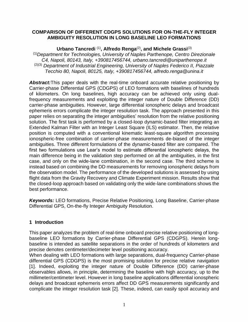
scheme are briefly recalled in the following, and the interested reader is referred to [8] for further details. In this mixed integer continuous dynamical filter (see Fig.1) the EKF is in charge of generating the float estimate, that is, the estimation of all the variables as real-valued, integer ambiguities included. Starting from the float estimate, the LAMBDA method [9] is used to conduct the integer searching step. The integer nature of the validated ambiguities is then exploited to correct the real-valued float estimate, yielding the fixed estimate. This is fed back to the EKF to improve the solution in the following time instants.

Figure 1. Schematic representation of the reference closed-loop EKF for CDGPS.

In real-time onboard relative positioning, where precise state initialization and high accuracy dynamic and stochastic models are typically not available [4], closed-loop schemes represent a reference method to keep the solution accurate. Specifically, this is achieved when correct integer ambiguities are used to calculate the fixed solution. However, depending on the estimated float ambiguities, and on the related covariance matrix, there is a non-null probability to compute wrong integer estimates. From a theoretical point of view, it is possible to show that, under the assumption of a Gaussian float estimate, the distribution of the integer estimates derived by LAMBDA is centered about the mean of the float ambiguity [10]. If the float ambiguity is assumed to be unbiased, its distribution is thus centered about the true integer value. As a consequence, the probability to derive wrong integer estimates is very low when the float distribution is sufficiently sharp w.r.t. the carrier wavelength and unbiased. This does not usually happen in real-world data, where the float ambiguity distribution can be both biased, converging to a non integer value, and not sharp enough. When large baseline applications are considered, this bias is dominated by uncompensated differential errors such as differential ionospheric delay [11] and differential broadcast ephemeris error. The capability of the EKF to yield accurate float ambiguity estimates in real-time onboard operation, when accurate ephemeris are not available, can be improved by modeling the ionospheric effect as part of the state vector. This is the approach adopted in the reference solution [8], based on Lear’s isotropic mapping function [12], which models the ratio of the slant Total Electron Content (TEC) to the vertical TEC (VTEC) as a function of the elevation on the horizon of GPS satellites as measured by GPS receivers.

With specific reference to a formation of two satellites, named chief and deputy, the EKF state vector of the reference solution is

4

8 2 1

1,Tp T T T T

wx x b VTEC a a (1)

where b’ includes the relative position vector, computed from the chief to the deputy, and the relative velocity vector in ECEF (Earth Centred Earth Fixed) reference frame, VTEC is the vector comprising the two vertical total electron contents above the receivers, aw and a1 represent the vector of wide-lane (WL) and L1 DD ambiguities, respectively. The corresponding EKF measurement vector is

4 1

1 2 1 2,TT T T T

p j j j jy y P P L L (2)

where 1

jP and 2

jP are DD pseudorange measurement vectors, and 1

jL and 2

jL are DD

carrier phase measurement vectors. The superscript j represents the reference GPS satellite, conventionally named pivot, and selected to calculate DD observables from undifferenced ones. In Eq. (1)-(2) p is the number of DD observations of each kind. The relative dynamic model relies on Keplerian relative orbital motion corrected with differential J2 effects. VTECs above the receivers are modeled as two scalar first-order Gauss-Markov processes with equal correlation time scale, whereas cycle ambiguities are modeled as random constant plus random walk processes. The utilization of two VTECs and Lear’s mapping function allows estimating all DD ionospheric delays as a function of only two variables: in this way the observability of the integer ambiguity by the reference solution is enhanced. Hence, the reference solution’s EKF non linear observation model y=h(x) can be written as

2

1

1

22 2

0 0

0 0

0

p p pp

p p ppj j

CD CD w

p p pp

p p pp

I I

I Ih x

I II

I I II

ρ b I VTEC a a (3)

where Ip is the p-dimensional identity matrix, j

CDρ is the vector of the DD signal paths for

all the visible GPS satellite vehicles, considering the pivot j, the chief satellite C and the

deputy satellite D,1 and 2 are L1 and L2 signal wavelength, 1 2 .

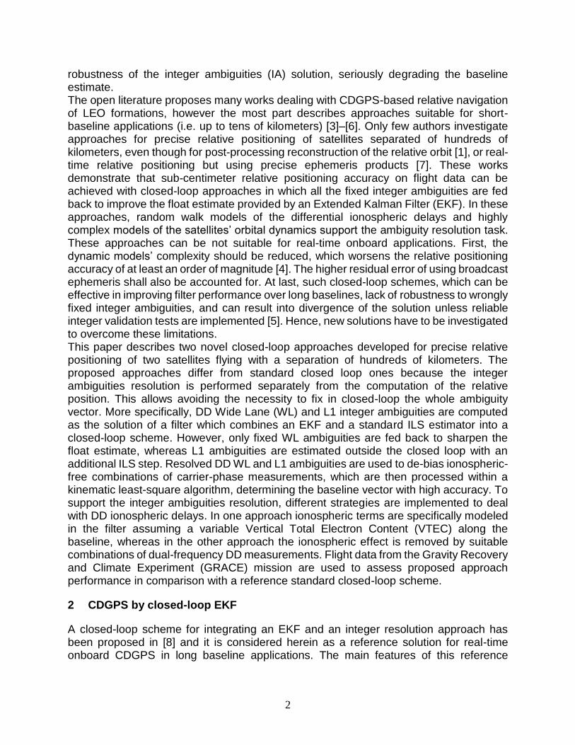
Figure 2 describes the reference strategy to derive the fixed solution. Wide-lane and L1 integer estimates derived by LAMBDA are screened by Partial Integer Validation (PIV) tests. In more detail, four different tests are used to validate the ambiguities. The first two tests scan WL integer estimates and the last two work on L1 ambiguities. A cascade strategy is implemented, i.e. L1 tests are performed only for those couples with validated WL ambiguity. The first WL test evaluates the instantaneous measurement residual of Melbourne-Wubbena observables [13] and is passed when the residual is lower than a pre-defined threshold. The second WL test checks the difference between the float and the integer estimates of wide-lane ambiguity. A similar approach is adopted to test L1 ambiguity using the ionospheric-free DD carrier-phase instantaneous measurement residual and the difference between the float and the integer value of narrow lane combination of WL and L1 ambiguity [8]

5

Validated ambiguities are used to compute the fixed solution, based on the correlation between the relevant float ambiguity and the remaining variables of the state vector [9]:

1ˆ ˆP P β β α α ; 1P P P P P

(4)

where the baseline vector β comprises all the state vector components but the validated ambiguities (both WL and L1) that are included in the vector α. The symbols ˆ and ˘ refer to the float and fixed estimates, respectively, and Pcd stands for the float covariance matrix between the generic variables c and d. As a consequence of the considered PIV strategy the closed-loop EKF has to deal with a mixed array of real-valued variables, fixed, and unfixed ambiguities, representing both not yet validated ambiguities and ambiguities related to newly acquired satellites.

Figure 2. Reference strategy for estimating the fixed solution and validated integer ambiguities.

In conclusion it is important to remark that, thanks to the validated ambiguities, the fixed solution is expected to be more accurate than the float one, thus improving the capability to correctly validate new ambiguities in the following time epochs. Nonetheless, the relative positioning accuracy of the fixed solution is still limited by the accuracy of Lear’s mapping function that can be poor, especially over polar areas [11]. For this reason, when at least four WL and L1 ambiguities (referring to the same DD couple of GPS Satellite Vehicles) are validated, the debiased ionospheric free combination of carrier-phase measurements is used to refine the relative positioning solution by a conventional Weighted Least-Squares Algorithm (WLSQ) as shown in Fig.1.

3 Alternative closed-loop schemes

The reference solution for CDGPS presented in the previous section has been tested on real world long-baseline spaceborne GPS measurements showing very good performance, characterized by root mean square (rms) baseline vector errors of few centimeters and maximum errors always smaller than one meter [8]. However, this performance cannot be always guaranteed for diverse operative conditions, such as ionospheric activity, observation geometry and so on. The reasons for this lack of robustness to different operative conditions deals with the feed-back logic and the considered ionospheric model.

6

Concerning the first point, the cascade validation of WL and L1 ambiguities represents an effective way to improve the accuracy of the fixed solution but it can be extremely sensitive to wrongly validated integer ambiguities. A very limited number of wrong ambiguities can cause the divergence of the closed-loop EKF solution. For this reason very restrictive thresholds must be set when performing the validation tests (especially for validating L1 ambiguities). This results in relatively low percentages of validated integers and therefore in degraded relative positioning accuracy under specific, very challenging, operative conditions. With reference to the ionospheric delays, it has been noted that some conditions exist in which the accuracy of Lear’s mapping function can be considered a limiting factor. On the contrary, it is well-known that, when dual-frequency measurements are available, as in semi-codeless GPS receivers, different measurement combinations can be used to remove the ionospheric contribution but preserving the integer nature of carrier-phase ambiguities. The following subsections focus on two alternative closed-loop EKF schemes aimed at coping with these critical aspects of the reference solution.

3.1 Wide-lane closed-loop EKF

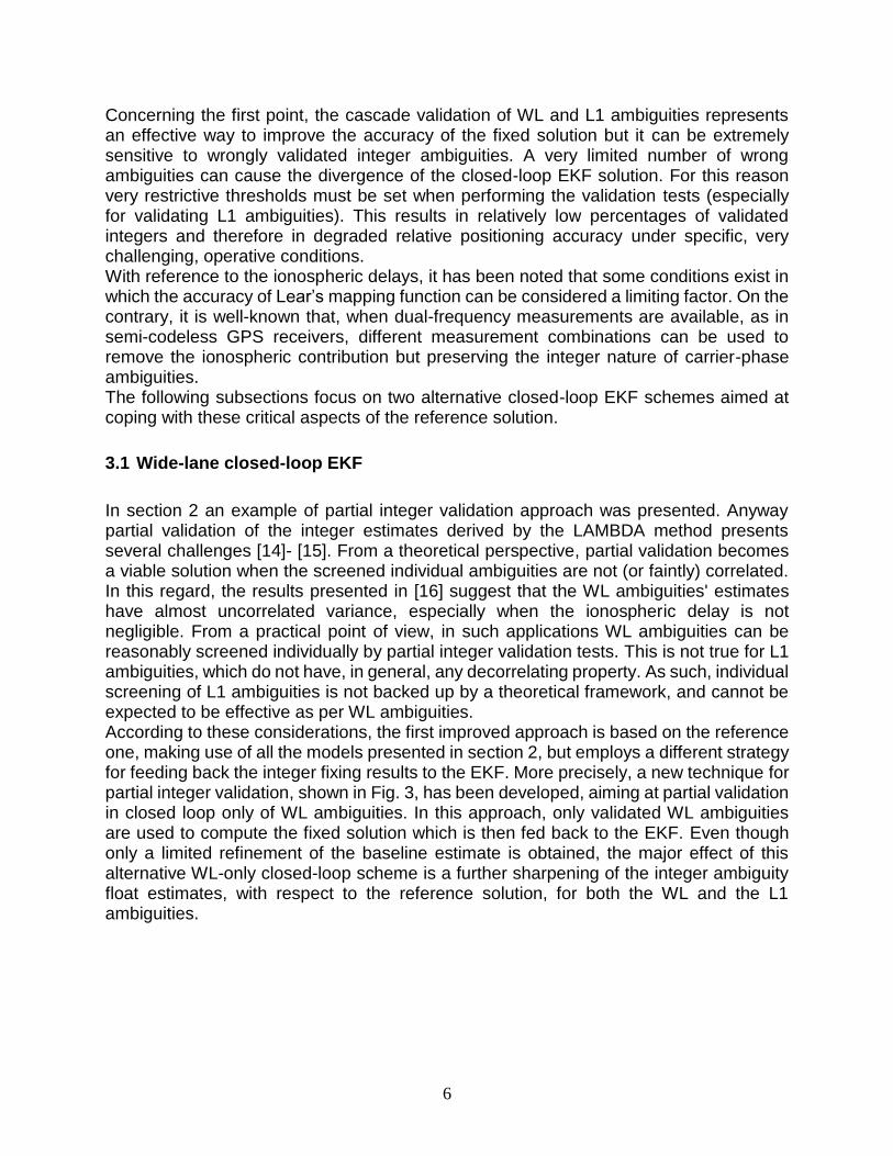
In section 2 an example of partial integer validation approach was presented. Anyway partial validation of the integer estimates derived by the LAMBDA method presents several challenges [14]- [15]. From a theoretical perspective, partial validation becomes a viable solution when the screened individual ambiguities are not (or faintly) correlated. In this regard, the results presented in [16] suggest that the WL ambiguities' estimates have almost uncorrelated variance, especially when the ionospheric delay is not negligible. From a practical point of view, in such applications WL ambiguities can be reasonably screened individually by partial integer validation tests. This is not true for L1 ambiguities, which do not have, in general, any decorrelating property. As such, individual screening of L1 ambiguities is not backed up by a theoretical framework, and cannot be expected to be effective as per WL ambiguities. According to these considerations, the first improved approach is based on the reference one, making use of all the models presented in section 2, but employs a different strategy for feeding back the integer fixing results to the EKF. More precisely, a new technique for partial integer validation, shown in Fig. 3, has been developed, aiming at partial validation in closed loop only of WL ambiguities. In this approach, only validated WL ambiguities are used to compute the fixed solution which is then fed back to the EKF. Even though only a limited refinement of the baseline estimate is obtained, the major effect of this alternative WL-only closed-loop scheme is a further sharpening of the integer ambiguity float estimates, with respect to the reference solution, for both the WL and the L1 ambiguities.

7

Figure 3. Alternative strategy for estimating the fixed solution and the integer ambiguities.

In more detail, L1 ambiguities corresponding to validated WL ambiguities and resulting from the application of Eq.(4), denoted as “fixed L1” in Fig.3, are processed by a secondary LAMBDA. The resulting L1 integer ambiguities are assumed valid and therefore ready to feed the WLSQ algorithm. Concerning this, it is important to note that the alternative WL-only closed-loop scheme is not sensitive to wrong estimates of L1 ambiguities, which are never fixed within the closed-loop EKF. From this point of view, it is potentially able to recover wrongly fixed L1 integer ambiguities, which are computed at each time step. Thus, it can be proved to be more robust than the reference solution.

3.2 Wide-lane closed-loop EKF without ionospheric delays

The second improved approach proposed in this paper further elaborates on the one presented in the previous section. In addition to providing WL-only feedback to the EKF, this approach also treats ionospheric delays in a different manner w.r.t. the reference one. The reference solution models DD ionospheric delays as a function of chief and deputy VTEC by Lear’s isotropic mapping function. For this model, RMS prediction errors in the order of few centimeters have been verified on large baseline satellite data [11]. However, the availability of dual-frequency GPS measurements makes it possible to form different measurement combinations that are able to remove completely the first-order ionospheric delay from the observation model, without the need of compensating it by estimation within the EKF state vector. In this section a different formulation of the closed-loop EKF is presented, processing only such “iono-removed” measurements. The state vector comprises thus only baseline, baseline rate, wide-lane, and L1 ambiguities, and its dynamics is governed by the same models of section 2, obviously excluding the VTEC ones.

6 2 1

1,Tp

wx x b a a (5)

For obtaining an observation model without ionospheric delays, suitable combinations of DD measurements must be selected. GPS measurement combinations which allow for an exact cancellation of first-order ionospheric delays can be classified in three main families: ionospheric-free combinations [17], GRoup And PHase Ionospheric Corrections (GRAPHIC) [18], and Melbourne-Wubbena combinations [13]. The ionospheric-free

8

combination (IF) is the most natural and diffuse combination for eliminating the ionospheric delay and it is based on combining observations of the same type on two carrier frequencies, exploiting the frequency dependence on the first-order ionospheric delay effect. With specific reference to the DD measurements reported in Eq.(2), two different ionospheric-free combinations can be derived, namely ionospheric-free combinations of pseudorange measurements and of carrier-phase measurements. GRAPHIC combinations exploit the asymmetry of the ionospheric effect on group and phase propagation at the same frequency. Again, two GRAPHIC combinations can be calculated considering L1 and L2 frequency, respectively. Finally, Melbourne-Wubbena combinations represent an estimate of WL ambiguities and cancel the ionospheric delays by combination of all four types of observables. These three families produce five types of combinations, which are not linearly independent. Specifically, only three are linearly independent and therefore there is the need of selecting the three combinations the EKF has to process. With the aim of guaranteeing an accurate estimation of the baseline vector, but also a satisfactory observability of the entire state vector, ionospheric-free combination of carrier-phase measurements LIF, GRAPHIC combination on L1 frequency G1, and Melbourne-Wubbena combination MW, are selected, which can be derived from uncombined DD observables as follows

2

1 22

1

1IF

L L L (6a)

1 1 10.5 G P L (6b)

1 2 1 2

1 2 1 2

w n

L L P PMW (6c)

where pivot satellite j is not reported for simplicity. Combining the above definitions with the reference observation model in Eq.(3), the combined measurement vector y′:=(LIF

T, G1

T, MWT)T can be related to the “iono-removed” state vector, y′ = ,h′(x′) as follows

11

2

11

11

02

0

pp

p

j

p CD p w p

p w pn

II

I

h x I I

I I

ρ b a a (7)

Starting from the specified dynamics and observation models, the iono-removed version of the closed-loop EKF (see Fig.1) can be implemented. With specific reference to the derivation of the fixed solution and the management of the integer ambiguities, the strategy presented in section 3.1 and outlined in Fig. 3 is assumed also for the iono-removed version of the closed-loop EKF, that is, only WL ambiguities are tested and, once validated, kept as integer deterministic parameters in the closed-loop EKF.

9

4 Performance comparison on flight data

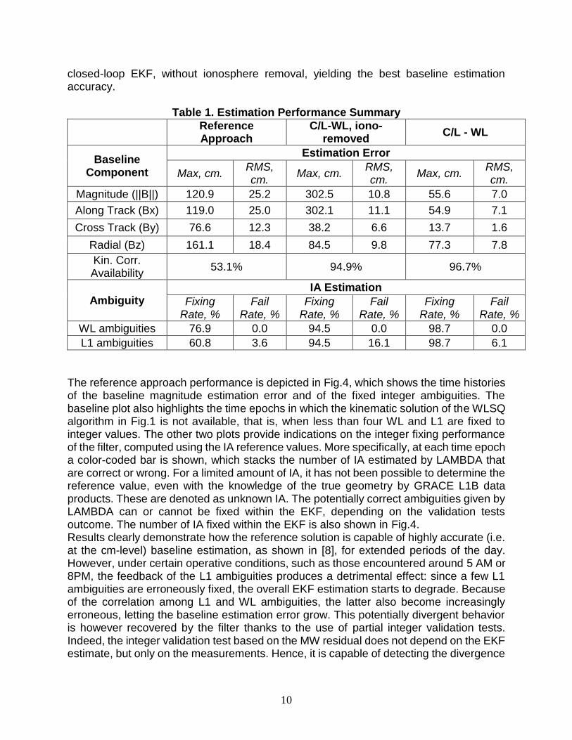
The performance of the three closed-loop algorithms is evaluated on actual flight data made available by the Gravity Recovery and Climate Experiment (GRACE) mission, which consists of two identical satellites, GRACE A and GRACE B, in a leader-follower formation using near circular orbits [19]. A one-day long dataset from DOY298, 2010 has been selected from all available GRACE Level-1 B (L1B) data for the analysis presented in this paper. The dataset comprises GPS L1B measurements at 0.1 Hz, Ka-Band Ranging System (KBR) data at 0.2 Hz , which allows estimating the true baseline at sub-millimeter accuracy, and GPS Navigation (GNV) L1B data at 1/60 Hz , which allows estimating the three-dimensional baseline in ECEF, but with a formal error in the order of few centimeters. As with all GRACE Level 1B data, the time-tags are corrected to GPS time using GPS clock solutions computed in post-processing [20]. A data-editing step has been performed on GPS L1B data in order to detect and remove outliers in the pseudorange measurements and to discard all observations from GPS satellites whose elevation above the local horizon is smaller than 10 deg. Estimation performance is quantified by comparing the baseline estimated by each filter to the reference solution obtained by KBR (for the magnitude) and GNV data (for the baseline vector components). Because of the different features of the data, the baseline magnitude estimation error can be quantified with very high accuracy, whereas estimation of the three-dimensional error is reliable only for error values at least in the order of 10 cm. For providing additional insight into filters' performance, their capability of fixing the correct integer ambiguities is also analyzed. For this purpose, reference values of the integer ambiguities have been computed by exploiting the knowledge of the observation geometry provided by the KBR and GNV data. The adopted procedure is described in [11], to which we refer the interested reader. For comparing the performance of different positioning solutions over the same dataset it is essential that the compared solutions approximate the maximum attainable navigation performance of each filter to the same extent. Indeed, the accuracy of relative positioning solutions of EKF-based closed-loop schemes is heavily dependant on the value chosen for the tunable parameters, especially when true flight data are involved [4]. Thus, quantifying the maximum attainable performance of each of the three filters requires optimizing the setting of the tunable parameters, which has been performed by a stochastic optimization technique. More precisely, we have searched for a filter setting maximizing a performance metric related to the baseline estimation error over the selected dataset applying a randomized algorithm proposed in [21], to which we refer the interested reader. This algorithm is based on sampling the performance metric f(p) by a Monte Carlo (MC) technique applied to the tunable parameters vector p. For applying the MC sampling technique, the parameter vector p is fictitiously modeled as a stochastic variable. The maximum performance is then estimated by the maximum value among f samples, which can be guaranteed (in a probabilistic sense) to approximate the true maximum to a finite extent, depending on the number of samples used in the MC technique. By tuning all three relative navigation filters with the same optimization algorithm, the performance comparison presented in the following is not biased towards one of the positioning solutions because of tuning effects. The estimation performance of the three approaches is summarized in Table 1. The reference filter performance is improved by both the proposed approaches, with the WL

10

closed-loop EKF, without ionosphere removal, yielding the best baseline estimation accuracy.

Table 1. Estimation Performance Summary

Reference Approach

C/L-WL, iono-removed

C/L - WL

Baseline Component

Estimation Error

Max, cm. RMS, cm.

Max, cm. RMS, cm.

Max, cm. RMS, cm.

Magnitude (||B||) 120.9 25.2 302.5 10.8 55.6 7.0

Along Track (Bx) 119.0 25.0 302.1 11.1 54.9 7.1

Cross Track (By) 76.6 12.3 38.2 6.6 13.7 1.6

Radial (Bz) 161.1 18.4 84.5 9.8 77.3 7.8

Kin. Corr. Availability

53.1% 94.9% 96.7%

Ambiguity IA Estimation

Fixing Rate, %

Fail Rate, %

Fixing Rate, %

Fail Rate, %

Fixing Rate, %

Fail Rate, %

WL ambiguities 76.9 0.0 94.5 0.0 98.7 0.0

L1 ambiguities 60.8 3.6 94.5 16.1 98.7 6.1

The reference approach performance is depicted in Fig.4, which shows the time histories of the baseline magnitude estimation error and of the fixed integer ambiguities. The baseline plot also highlights the time epochs in which the kinematic solution of the WLSQ algorithm in Fig.1 is not available, that is, when less than four WL and L1 are fixed to integer values. The other two plots provide indications on the integer fixing performance of the filter, computed using the IA reference values. More specifically, at each time epoch a color-coded bar is shown, which stacks the number of IA estimated by LAMBDA that are correct or wrong. For a limited amount of IA, it has not been possible to determine the reference value, even with the knowledge of the true geometry by GRACE L1B data products. These are denoted as unknown IA. The potentially correct ambiguities given by LAMBDA can or cannot be fixed within the EKF, depending on the validation tests outcome. The number of IA fixed within the EKF is also shown in Fig.4. Results clearly demonstrate how the reference solution is capable of highly accurate (i.e. at the cm-level) baseline estimation, as shown in [8], for extended periods of the day. However, under certain operative conditions, such as those encountered around 5 AM or 8PM, the feedback of the L1 ambiguities produces a detrimental effect: since a few L1 ambiguities are erroneously fixed, the overall EKF estimation starts to degrade. Because of the correlation among L1 and WL ambiguities, the latter also become increasingly erroneous, letting the baseline estimation error grow. This potentially divergent behavior is however recovered by the filter thanks to the use of partial integer validation tests. Indeed, the integer validation test based on the MW residual does not depend on the EKF estimate, but only on the measurements. Hence, it is capable of detecting the divergence

11

of the WL estimate, and eventually to recover it as the operating conditions become again favorable.

Figure 4. Reference approach performance: baseline norm estimation error (top),

WL (middle) and L1 (bottom) IA fixing.

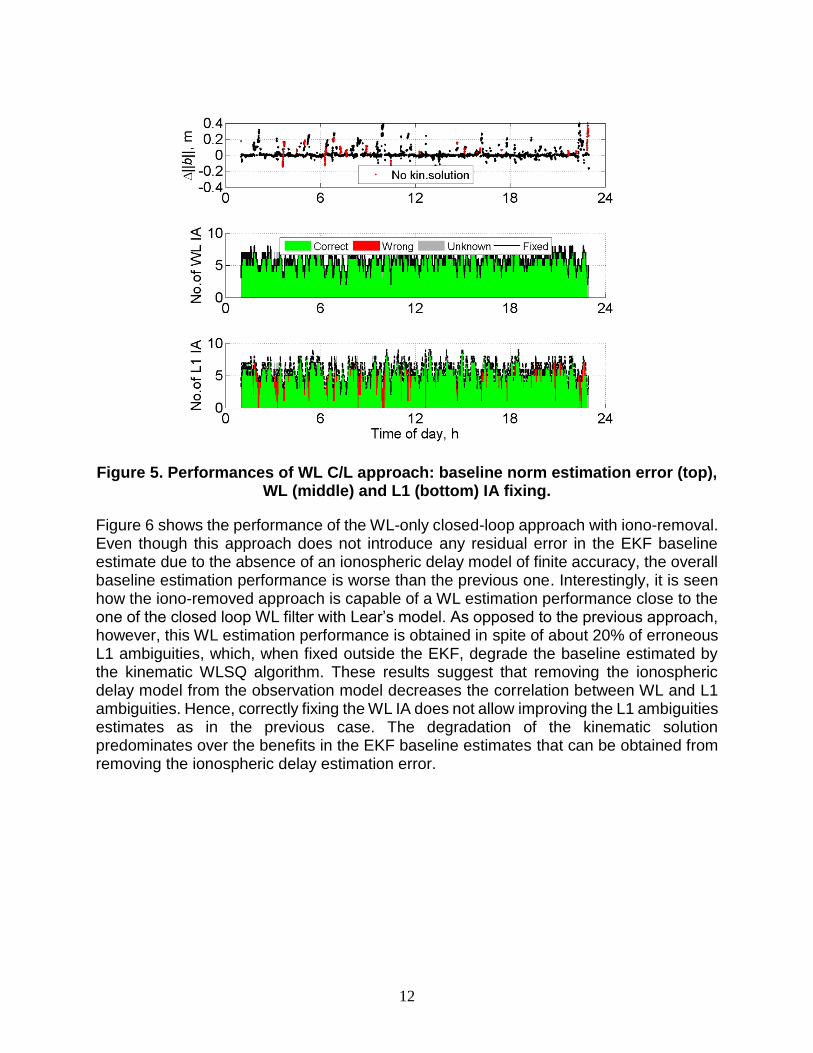
Figure 5 shows the same results, but computed for the closed-loop approach in which only the WL integer ambiguities are fed back to the EKF and the differential ionospheric delay is specifically modeled. The baseline estimation performance is substantially improved with respect to the reference approach. The baseline estimation performance of the two filters is similar in the periods in which the reference approach yields a sharp estimate (e.g. around noon). However, the WL-only approach is more robust to the changing operating conditions, being capable of preserving a centimeter level accuracy throughout the dataset. This improvement is possible thanks to the capability of fully exploiting the mostly correct WL LAMBDA estimates. Indeed, the lack of erroneously fixed L1 ambiguities within the EKF allows relaxing the PIV tests for letting more WL ambiguities being fixed, which increase to almost 100% from the ~80% of the reference solution (see Table 1). This has a beneficial effect also on the quality of the L1 LAMDA estimates, which, as shown in Fig.5, are mostly correct. Recall that only the L1 ambiguities that have a valid WL counterpart are fixed to the relevant integer value. Moreover, such L1 IA are used only for computing the kinematic solution, but not for modifying the EKF estimate at later time instants (see Fig.3). Therefore their number is denoted by a dashed line in Fig.5.

12

Figure 5. Performances of WL C/L approach: baseline norm estimation error (top),

WL (middle) and L1 (bottom) IA fixing.

Figure 6 shows the performance of the WL-only closed-loop approach with iono-removal. Even though this approach does not introduce any residual error in the EKF baseline estimate due to the absence of an ionospheric delay model of finite accuracy, the overall baseline estimation performance is worse than the previous one. Interestingly, it is seen how the iono-removed approach is capable of a WL estimation performance close to the one of the closed loop WL filter with Lear’s model. As opposed to the previous approach, however, this WL estimation performance is obtained in spite of about 20% of erroneous L1 ambiguities, which, when fixed outside the EKF, degrade the baseline estimated by the kinematic WLSQ algorithm. These results suggest that removing the ionospheric delay model from the observation model decreases the correlation between WL and L1 ambiguities. Hence, correctly fixing the WL IA does not allow improving the L1 ambiguities estimates as in the previous case. The degradation of the kinematic solution predominates over the benefits in the EKF baseline estimates that can be obtained from removing the ionospheric delay estimation error.

13

Figure 6. Performances of WL C/L approach without ionospheric delays: baseline

norm estimation error (top), WL (middle) and L1 (bottom) IA fixing.

5 Conclusion

This paper has focused on CDGPS-based real-time onboard relative navigation of two LEO GPS receivers separated of hundreds of kilometers. State of the art approaches for this problem rely on closed-loop dynamic filtering schemes which integrate an EKF with an integer estimator to fix the carrier-phase ambiguities to their unknown integer values. In closed-loop approaches, fixed integers are feed-back to the EKF with the aim of improving the EKF estimate at later time instants. However, wrongly-fixed integer ambiguities may cause divergence of the estimates. To highlight shortcomings of reference approaches, the performance of a closed-loop, relative navigation filter has been investigated using flight data from the GRACE mission. Although a decimeter-level accuracy can be achieved in the baseline estimation, this performance cannot be maintained under demanding operative conditions, present in the analyzed dataset. The baseline estimation error indeed grows due to the feeding back to the EKF of erroneously-fixed L1 ambiguities. Nonetheless, a careful design of the integer validation strategy allows the filter to recover from this performance degradation as the operative conditions become again more favorable. To increase the robustness of the reference solution to the variability of operative conditions two approaches have been proposed and investigated in the paper. To limit the detrimental effect on filter performance of the erroneous L1 ambiguities, these last ones are fixed to integer values outside the EKF, thus feeding back only fixed integer solutions of wide-lane ambiguity combinations. The effectiveness of this approach is

14

demonstrated by the increase of the percentage of correctly fixed ambiguities of more than 20 % with respect to the reference approach, thus improving the baseline estimation RMS error of a factor of three. Compensation of the double-difference ionospheric delays is known to be one of the limiting factors in relative positioning over large baselines. In the two proposed approaches this problem is faced in two different ways: using a ionospheric delay model of centimeter-level accuracy, in one case, and exactly canceling first-order ionospheric effects by suitable combinations of double-difference measurements, in the other case. Results show that removing the ionospheric delays from the observation model decreases the correlation between WL and L1 ambiguities. Hence, the latter do not benefit from the WL feedback as when using a ionosphere delay model, being erroneously computed in about 10% more cases. The resulting degradation of the kinematic solution predominates over the benefits in the EKF baseline estimates that can be obtained by removing the ionospheric delay estimation error.

References

[1] R. Kroes, O. Montenbruck, W. Bertiger, P. Visser, Precise GRACE baseline determination using GPS, GPS Solutions, Volume 9, Issue 1, pp 21-31, April 2005.

[2] U. Tancredi, A. Renga, M. Grassi, Carrier-based Differential GPS for autonomous relative navigation in LEO, AIAA Guidance Navigation and Control Conference, August 2012, 11 pp., paper id AIAA-2012-4707.

[3] Montenbruck O. et all, Carrier Phase Differential GPS for LEO Formation Flying - The PRISMA and TanDEM-X Flight Experience, Astr.Sp.Conf, 2011

[4] D'Amico, S., Ardaens, J. S., and Larsson, R. Spaceborne Autonomous Formation-Flying Experiment on the PRISMA Mission, Journal of Guidance Control and Dynamics Vol.35 no.3, 2012. pp.834-850.

[5] S. Leung, O. Montenbruck, Real-Time Navigation of Formation-Flying Spacecraft Using Global-Positioning-System Measurements, Journal Of Guidance, Control, And Dynamics, Vol. 28, No. 2, March–April 2005, pp. 226-235.

[6] Ebinuma, T., Bishop, R.H. and Glenn Lightsey, E. Integrated hardware investigations of precision spacecraft rendezvous using the global positioning system, Journal of Guidance Control and Dynamics 26, no. 3, 2003. pp. 425-433.

[7] S.-Ch.Wu, Y.E. Bar-Sever, Real-time sub-cm differential orbit determination of two Low-Earth Orbiters with GPS bias fixing; ION GNSS 2006; September 26-29, 2006 Fort Worth, Texas, 2006.

[8] U. Tancredi, A. Renga, M. Grassi, Validation on flight data of a closed-loop approach for GPS-based relative navigation of LEO satellites, Acta Astronautica Vol. 86, pp. 126-135, 2013.

[9] Teunissen PJG (1995), The least-squares ambiguity decorrelation adjustment: a method for fast GPS integer ambiguity estimation. Journal of Geodesy, Vol.70, pp. 65-82.

15

[10] S. Verhagen, The GNSS integer ambiguities: estimation and validation, Ph.D. Thesis, Delft TU, 2005.

[11] U. Tancredi, A. Renga, M. Grassi, “Ionospheric path delay models for spaceborne GPS receivers flying in formation with large baselines”, Advances in Space Research, Vol. 48, No. 3, pp. 507–520, August 2011.

[12] W.M. Lear, GPS navigation for low-earth orbiting vehicles, NASA Lyndon B. Johnson Space Center, Mission planning and analysis division, 1st revision, NASA 87-FM-2, JSC-32,031, 1988.

[13] Melbourne, W.G. (1985), The case for ranging in GPS-based geodetic systems, in Proceedings of the 1st Intenational Symposium on Precise positioning with the Global Positioning System, pp. 373–386, Rockville, Maryland.

[14] Tancredi U., Renga, A., and Grassi, M., “GPS-Based Relative Navigation of LEO Formations with Varying Baselines,” AIAA Guidance, Navigation, and Control Conference, Toronto, Canada, August 2010.

[15] Teunissen P, Verhagen S (2007) GNSS carrier phase ambiguity resolution: challenges and open problems. In: Proceedings of the scientific meetings of the IAG general assembly 2007. Perugia, Italy.

[16] Teunissen, P.J.G. On the GPS widelane and its decorrelating property, Journal of Geodesy, 1997, Volume 71, Issue 9, pp 577-587

[17] J. Farrel , M. Barth, The Global Positioning System and Inertial Navigation, McGraw-Hill, New York, ch. 5, 1999.

[18] Yunck, T. P. Orbit determination, in: Parkinson B.W., Spilker, J.J. (eds), Global positioning system: theory and applications, vol. 2, American Institute of Aeronautics and Astronautics Inc., Washington, pp. 559-592, 1996

[19] Tapley, B. D., Bettadpur, S., Watkins, M., Reigber, C. The gravity recovery and climate experiment mission overview and early results, Geophys. Res. Lett., 31, L09607, 2004.

[20] Case, K., Kruizinga, G., Wu, S.C. GRACE level 1B data product user handbook, NASA Jet Propulsion Laboratory, revision 1.3, JPL D-22027, GRACE 327-733, 2010.

[21] Calafiore, G., Dabbene, F., Tempo, R.,A survey of randomized algorithms for control synthesis and performance verification, Journal of Complexity 23 (2007) 301 – 316