comparative study of forward and backward test-kinetic ... · comparative study of forward and...

ManuscriptpublishedtoComputerPhysicsCommunicationsComputerPhysicsCommunications183(2012)2561–2569;doi:10.1016/j.cpc.2012.07.005

1

Comparative study of forward and backward test-kinetic simulation approaches

Gabriel Voitcua,b, Marius Echima,c and Richard Marchandd aInstitute of Space Science, Atomistilor 409, Magurele 077125, Romania

bUniversity of Bucharest, Faculty of Physics, Atomistilor 405, Magurele 077125, Romania cBelgian Institute for Space Aeronomy, Avenue Circulaire 3, Brussels B-1180, Belgium

dUniversity of Alberta, Department of Physics, T6G 2G7 Edmonton, Alberta, Canada

Corresponding author: Gabriel Voitcu ([email protected])

Abstract

In this paper we perform a comparative study of the forward and backward Liouville

mapping applied to the modeling of ring-shaped and non-gyrotropic velocity distribution

functions of particles injected in a sheared electromagnetic field. The test-kinetic method is

used to compute the velocity distribution function in various areas of a proton cloud moving

in the vicinity of a region with a sharp transition of the magnetic field and a non-uniform

electric field. In the forward approach the velocity distribution function is computed for a

two-dimensional spatial bin, while in the backward approach the distribution function is

averaged over a spatial bin with the same size as for the forward method and using a two-

dimensional trapezoidal integration scheme. It is shown that the two approaches lead to

similar results for spatial bins where the velocity distribution function varies smoothly. On

the other hand, with bins covering regions of configuration space characterized by sharp

spatial gradients of the velocity distribution function, the forward and backward approaches

will generally provide different results.

Keywords: test-kinetic simulations, Liouville mapping, velocity distribution function, space

plasma.


2

1. Introduction

Test-kinetic simulations provide a useful tool to investigate the dynamics of charged

particles in systems in which a good approximation of the actual electromagnetic fields can

be obtained [1]. This approach can provide useful information about the kinetic structure of

the system. The electric and magnetic fields used in the test-kinetic approach are prescribed a

priori. Thus, the test-kinetic method gives a first approximation of the kinetic structure of a

plasma using electric and magnetic fields obtained from either theoretical models, MHD

simulations or experimental data. Although the results obtained using this approach are not

self-consistent, the test-kinetic method is an important simulation tool able to provide a useful

description of complex situations where the use of self-consistent kinetic methods is not

possible.

The test-kinetic method has been applied in various contexts of space plasma physics.

For example, Wagner et al. [2] integrated test-particle orbits in an X-line distribution of the

magnetic field illustrating the non-adiabatic character of orbits for sheets having the thickness

comparable with the particle’s Larmor radius. Speiser et al. [3] used the test-kinetic approach

to map velocity distribution functions from the magnetosphere into the magnetosheath.

Curran et al. [4] and Curran and Goertz [5] mapped velocity distribution functions along

numerically integrated orbits in order to study the plasma dynamics in X-line magnetic

topology. Ashour-Abdalla et al. [6] investigated the ion dynamics into the magnetotail using

the test-kinetic approach. Richard et al. [7] studied the magnetospheric penetration

mechanisms by solar wind ions using the same method, for electric and magnetic field

profiles obtained from a global MHD simulation of the terrestrial magnetosphere. Rothwell et

al. [8] developed test-particle simulations in order to investigate non-adiabatic effects

introduced by sharp spatial variations of the electromagnetic field. Delcourt et al. [9,10,11]

performed test-particle simulations to investigate impulsive changes of ion dynamics in the

near-Earth plasma sheet. Mackay et al. [12] and Marchand et al. [13] applied the test-kinetic

approach to obtain first order kinetic effects in collisionless perpendicular shocks in the

vicinity of the Earth’s bow shock and also to check consistency with a solution obtained in

the MHD approximation.

The test-kinetic simulation method is based on numerical integration of test-particle

orbits in prescribed electric and magnetic fields. Marchand [1] identified four different

approaches of the test-kinetic method: (i) trajectory sampling, (ii) forward Monte Carlo, (iii)

forward Liouville and (iv) backward Liouville. In this paper we perform a comparative study


3

of the forward and backward Liouville approaches in the test-kinetic modelling of ring-

shaped and non-gyrotropic velocity distribution functions for particles injected in a sheared

electromagnetic field. The test-kinetic simulation method is used to compute the velocity

distribution function in various regions of a proton cloud moving in the vicinity of a region

with a sharp transition of the magnetic field. This type of configuration is of interest for

studying the dynamics of the terrestrial magnetotail. The distribution functions obtained with

both approaches are compared and the differences are analyzed.

The remainder of the paper is organized as follows. In the second section we outline

the main features of both forward and backward test-kinetic approaches and describe how

they are applied in our simulations. In the third section we illustrate the numerical solutions

obtained for a cloud of protons injected in a non-uniform electromagnetic field and we

analyze the differences between the velocity distribution functions given by both approaches.

The last section includes our conclusions.

2. Test-kinetic modeling: forward and backward Liouville approaches

In a collisionless plasma the characteristics of the Vlasov equation can be obtained by

solving the Newton-Lorentz equation of motion:

d 2!rdt2 = q

m!E + d!r

dt×!B⎛

⎝⎜⎞⎠⎟

(1)

for an ensemble of charged particles injected into the electromagnetic field given by !E and

!B [14]. This is equivalent to Liouville’s theorem applied to a one-particle distribution

function which states that:

0dfdt

= (2)

along a particle trajectory. Therefore, the velocity distribution function has the same

numerical value at each point along a particle orbit. One can compute any number of Vlasov

characteristics and then “propagate” f along them by applying Liouville’s theorem.

In the forward and backward test-kinetic approaches the magnetic and electric fields

introduced in Eq. (1) are prescribed. The B-field used in our computations is stationary and it

varies with the x-coordinate in a transition region centred at x=0. The profile of the magnetic

field is anti-parallel, i.e. !B is everywhere parallel to the z-axis and it changes orientation as it

goes through x=0:


4

1( ) erfz zxB x BL

⎛ ⎞= − ⎜ ⎟⎝ ⎠ (3)

where B1z represents the asymptotic field in the left hand side of the transition region

(x→−∞), −B1z is the asymptotic field in the right hand side (x→+∞) and L represents the

characteristic scale length of the transition region. This type of magnetic profile has been

obtained self-consistently from kinetic models of one-dimensional tangential discontinuities

[15,16,17].

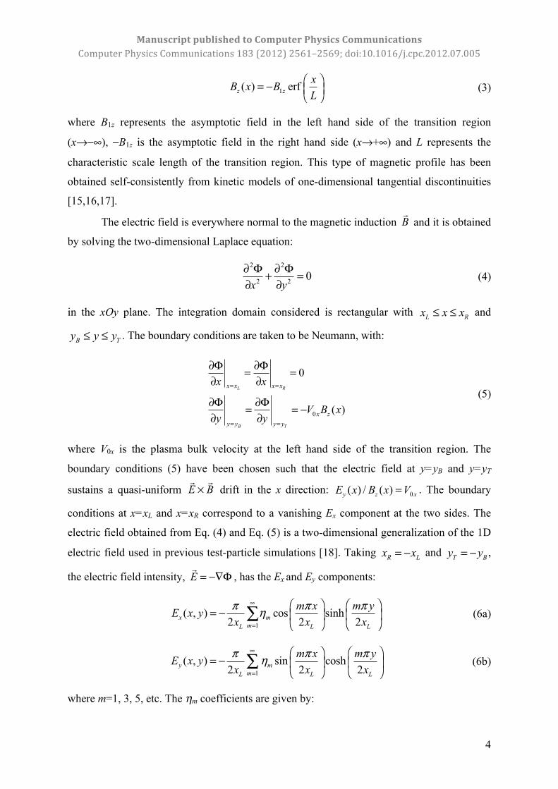
The electric field is everywhere normal to the magnetic induction !B and it is obtained

by solving the two-dimensional Laplace equation:

2 2

2 2 0x y

∂ Φ ∂ Φ+ =∂ ∂

(4)

in the xOy plane. The integration domain considered is rectangular with L Rx x x≤ ≤ and

B Ty y y≤ ≤ . The boundary conditions are taken to be Neumann, with:

0

0

( )

L R

B T

x x x x

x zy y y y

x x

V B xy y

= =

= =

∂Φ ∂Φ= =∂ ∂

∂Φ ∂Φ= = −∂ ∂

(5)

where V0x is the plasma bulk velocity at the left hand side of the transition region. The

boundary conditions (5) have been chosen such that the electric field at y=yB and y=yT

sustains a quasi-uniform !E ×!B drift in the x direction: 0( ) / ( )y z xE x B x V= . The boundary

conditions at x=xL and x=xR correspond to a vanishing Ex component at the two sides. The

electric field obtained from Eq. (4) and Eq. (5) is a two-dimensional generalization of the 1D

electric field used in previous test-particle simulations [18]. Taking R Lx x= − and T By y= − ,

the electric field intensity, !E = −∇Φ , has the Ex and Ey components:

1

( , ) cos sinh2 2 2x m

mL L L

m x m yE x yx x xπ π πη

∞

=

⎛ ⎞ ⎛ ⎞= − ⎜ ⎟ ⎜ ⎟

⎝ ⎠ ⎝ ⎠∑ (6a)

1

( , ) sin cosh2 2 2y m

mL L L

m x m yE x yx x xπ π πη

∞

=

⎛ ⎞ ⎛ ⎞= − ⎜ ⎟ ⎜ ⎟

⎝ ⎠ ⎝ ⎠∑ (6b)

where m=1, 3, 5, etc. The ηm coefficients are given by:


5

0 1

2

2 2erf sin( )cosh

2

L x z Lm

B

L

x V B x m dLm y

x

π

π

η θ θ θπππ

+

−

⎛ ⎞= ⎜ ⎟⎛ ⎞ ⎝ ⎠⎜ ⎟⎝ ⎠

∫ (7)

The solution of Laplace’s equation (4) with boundary conditions (5) may be viewed as an

electric field simulating the one sustained by space-charge layers forming at the boundaries

of a moving non-diamagnetic plasma element in the presence of a magnetic field [19,20]. Our

simulations have been performed for an electromagnetic field configuration that reproduces

some typical parameters of the terrestrial magnetotail. The magnetic field profile would

correspond to a tangential discontinuity. A possible origin of the electric field can be a

localized perturbation of the dawn-dusk electric field. Another region of the magnetosphere

where such electric and magnetic fields could be observed is the magnetopause. The

relevance for this configuration of the electric and magnetic fields have been discussed in a

previous publication [21].

The initial velocity distribution function specified for the source region is described

by a displaced Maxwellian with the average velocity !

V0 parallel to the positive x-axis and

perpendicular to the magnetic field:

2 2 20

0

( )3/ 22

00

( , , )2

x y z

B

m v V v v

k Tx y z

B

mf v v v N ek Tπ

⎡ ⎤− + +⎣ ⎦−⎛ ⎞= ⎜ ⎟

⎝ ⎠ (8)

where N0 and T0 are the density and temperature of protons at the source region. In both

forward and backward approaches the initial (t=0) source region, where the velocity

distribution function is known, is localized in the left hand side of the transition region in the

xOy plane. It is defined in terms of the positions of the guiding centers.

In the forward approach a uniform grid of guiding centers having Nx×Ny nodes is

placed inside the source region. For each of the Nx×Ny guiding centres, np particles are

“attached” with the initial velocities 0 0 0( , , )i i ix y zv v v distributed according to the displaced

Maxwellian (8). Knowing the gyration velocity and the guiding center position of all test-

particles, obtaining the particles’ position is straightforward. In order to reconstruct the

velocity distribution function at later times, 6×np×Nx×Ny equations of motion (1) are

numerically integrated in the time range t>0, thus providing 3×np×Nx×Ny components of the

test-particles velocities ( , , )i i ix y zv v v at time t . These final velocities define a scattered

distribution of points in velocity space. Using the Liouville theorem (2) we assign to each


6

point defined by the final velocities, ( , , )i i ix y zv v v , the numerical value of the distribution

function computed from (8) for the initial velocity components 0 0 0( , , )i i ix y zv v v . In this way we

obtain a map of f in the three-dimensional velocity space. This procedure is applied at time

t in those spatial bins of the configuration space populated by a sufficiently large number of

particles so as to have a good representation of f . A schematic diagram describing the

forward approach is shown in Fig. 1.

With the backward approach, a three-dimensional velocity grid ( , , )i i ix y zv v v with Nv

vertices is constructed at a precise position in configuration space. Starting from each vertex

of the velocity grid, the equation of motion of a test-particle is integrated backward in time

back to t=0. To each node of the grid a single test-particle is assigned. In order to reconstruct

the velocity distribution function at time t , 6×Nv equations of motion (1) are numerically

integrated backward in time, thus providing 3×Nv components 0 0 0( , , )i i ix y zv v v of the test-

particles velocities at time t=0 . If the particle’s i guiding center is localized inside the source

region, at time t=0, we assign to that particle the numerical value of the distribution function

computed from (8) for the velocity components 0 0 0( , , )i i ix y zv v v . Otherwise, the value of f is

set to zero. Using Liouville’s theorem (2) we assign to each vertex of the grid, ( , , )i i ix y zv v v , the

numerical value of the distribution function assumed at time t=0 . In this way f is

discretized in the three-dimensional velocity space. This procedure is applied at time t for Nr

points of interest in configuration space. A schematic diagram describing the backward

approach is shown in Fig. 2.

The numerical method used to solve the equation of motion of test-particles is based

on the 4th order Runge-Kutta algorithm with fixed step-size. We checked the accuracy of the

Runge-Kutta solver by integrating a number of 27 test-orbits with different initial conditions,

forward and backward in time, over an interval of 225 seconds (~100 Larmor periods) using

1500 time steps. The results obtained show that the error in computing the particles positions

is smaller than 0.13RL, while the error in computing the particles velocities is smaller than

0.10w⊥, where RL is the Larmor radius and w⊥ is the gyration velocity of the particles. These

results indicate that the accuracy of the numerical method used to integrate test-trajectories is

satisfactory.


7

3. Numerical results and comparison between forward and backward test-kinetic

approaches

The velocity distribution function is determined with the forward and backward test-

kinetic approaches for different regions of a proton cloud moving in an anti-parallel magnetic

field and a non-uniform electric field. The injection source is localized at the left hand side of

the transition region and it is characterized by the displaced Maxwellian (8). The input

parameters are given in Table I. The simulation domain is delimited by the interval [−40000,

+40000] km along the x-axis and [−30000, +30000] km along the y-axis. The particles that

reach regions outside these limits are removed from the simulation and no new particles are

injected at the boundaries. In the forward approach, a uniform grid of 12×12 nodes

considered as guiding centers is defined inside the source region; 20000 protons are

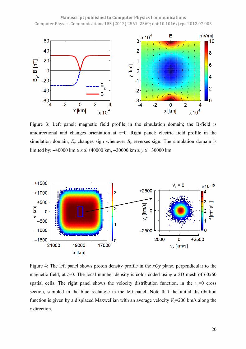
“attached” to each guiding center position. The magnetic field, described by Eq. (3), is

everywhere parallel to the z-axis and changes sign at x=0 (see Fig. 3 – left panel). Figure 3

(right panel) shows the electric field profile obtained from the Laplace equation (4) subject to

boundary conditions (5) discussed in the previous section. This profile may be viewed as

describing a neutral sheet and a superimposed electric field with Ey changing sign whenever

Bz reverses sign.

Figure 4 (left panel) shows the initial positions of protons (t=0) and the local number

density in the xOy plane, perpendicular to the magnetic field. A two-dimensional cross-

section (for vz=0) of the velocity distribution function corresponding to the central region (the

blue rectangle in the xOy plane) is shown in the right panel of Fig. 4. It is shown that the

initial distribution function is a displaced Maxwellian with an average velocity V0=200 km/s

in the x direction.

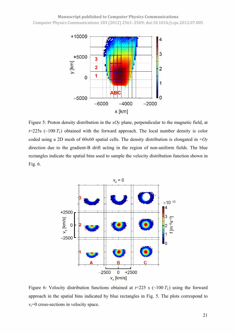
The positions and the local number density of the test-protons in the xOy plane,

perpendicular to the magnetic field, at t=225 s (∼100⋅TL) are shown in Fig. 5. The overall

shape of the proton cloud is deformed and shows significant asymmetries, the particles being

scattered in the positive direction of the y-axis. This asymmetric expansion of the cloud is

related to the gradient-B drift that is oriented in the +Oy direction. Thus, an energy-dispersed

structure is formed due to the energy-dependent displacement of protons towards the edges of

the cloud by the gradient-B drift. Another effect of the gradient-B drift is the formation of

ring-shaped velocity distribution functions within the energy-dispersed structure, as can be

seen further. Higher energy particles populate the edges of the proton beam while smaller

energies are located inside the core. Also, non-gyrotropic velocity distribution functions form

in the front-side and trailing edge of the cloud due to remote sensing of energetic particles


8

with guiding centers localized inside the beam. An explanation of the physical mechanism

responsible for the formation of such an energy-dispersed structure and also a detailed

analysis of the kinetic effects contributing to the formation of ring-shaped and non-gyrotropic

velocity distribution functions is published elsewhere [21]. Here we limit our attention to the

differences between the results obtained using both forward and backward test-kinetic

approaches.

The velocity distribution function of protons obtained at t=225 s using the forward

approach is shown in Fig. 6. The velocity distribution function inside the cloud is computed

for each bin defined by the blue rectangles in the xOy plane and identified by the combination

of letters (columns) and numbers (rows) in Fig. 5. The size of a spatial bin is defined such

that it contains enough particles (at least 104 particles per bin) for a good sampling of velocity

space. The bins of the mesh shown in Fig. 5 have a spatial resolution of 280 km in x-direction

and 2500 km in y-direction, adapted to the geometry of the cloud and the total number of

simulated particles. The corresponding velocity distribution functions obtained using the

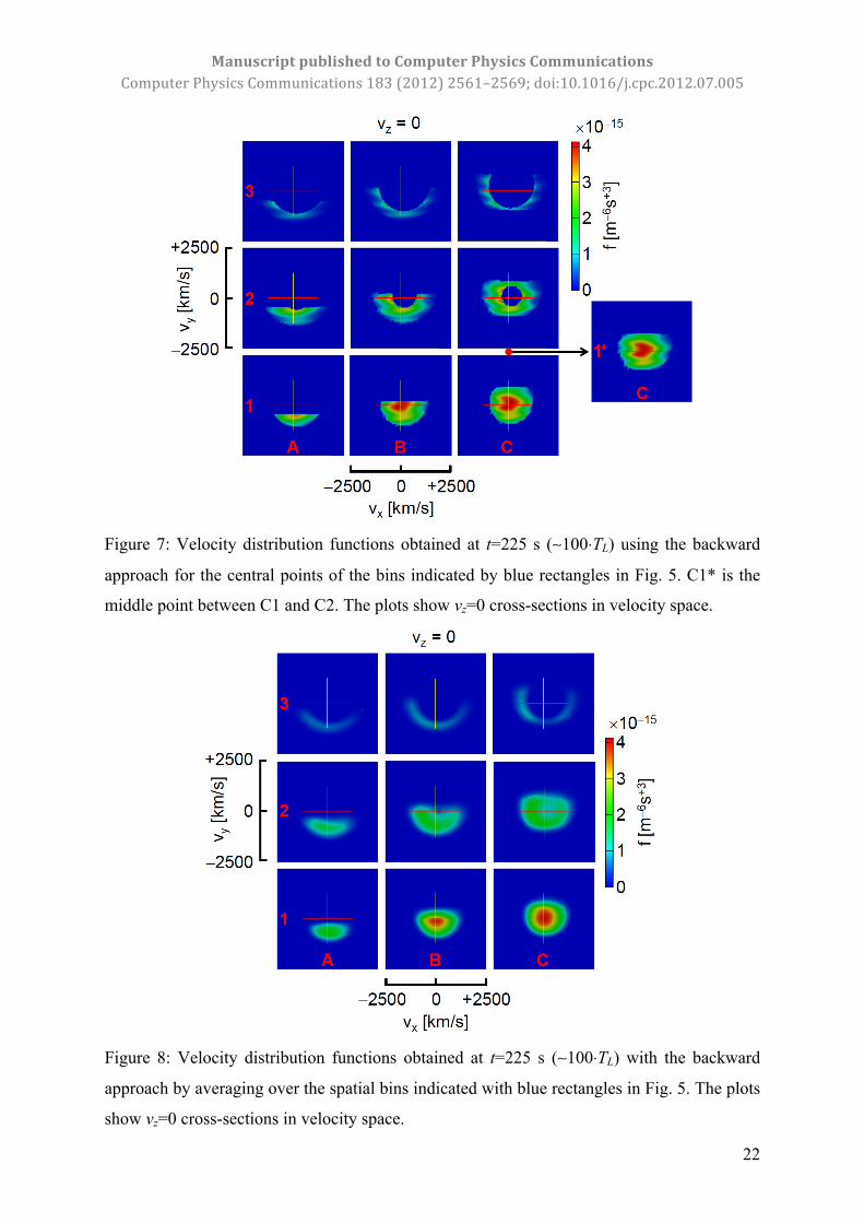
backward approach are shown in Fig. 7. f is computed for the central point of each spatial

bin defined by the blue rectangles in the xOy plane illustrated in Fig. 5.

There are significant differences between the forward and backward approaches as

illustrated by Fig. 6 and Fig. 7. Nevertheless, the velocity distribution function, f , has the

same variation tendency in both cases, i.e. (i) it is ring-shaped close to the upper boundary

(i.e. for larger y-values) while in the center is approximately Maxwellian (comparing, for

instance, f corresponding to C1 and C3 in Fig. 6 and Fig. 7) and (ii) the anisotropy of the

velocity distribution function is more pronounced close to the trailing edge of the cloud (i.e.

for smaller x-values) than in the center (for example, comparing f for A2 and B2 in Fig. 6

and Fig. 7). The explanation for the differences observed is related to the different methods

used to compute the distribution function with forward and backward approaches. In the

forward approach f is sampled over a spatial bin whose size is defined such that it contains

a large enough number of particles and the statistical error resulting from sampling is

minimized. On the other hand, in the backward approach the computation of f for a precise

point in configuration space is free from statistical errors; in our case, f is computed for the

central point of each spatial bin defined for the forward method. The strength of the backward

approach is related to its ability to produce detailed velocity distribution functions at precise

locations without statistical sampling errors. The essential difference between the forward

and backward approaches is that the former necessarily relies on spatial binning and


9

sampling, while the latter can be calculated at precise locations in space. In many cases, the

backward approach can lead to filamentary structures in velocity (or momentum) space,

while such structures are always attenuated in the forward approach, owing to the spatial

averages involved. In contrary to the backward approach, the forward Liouville approach

enables the computation of both the velocity distribution function and general dynamics of

the particle cloud while advancing an initial distribution of particles into a non-uniform

configuration of the magnetic and electric fields. Thus, the strength of the forward approach

is related to its ability to investigate the evolution of a specific plasma source.

A solution to eliminate these differences and to obtain comparable distribution

functions would involve spatial averages of f by a proper quadrature scheme applied in the

backward approach. For that purpose, the velocity distribution function obtained using the

backward approach is numerically integrated over a rectangular domain in the xOy plane

corresponding to the spatial bin used to compute the distribution function using the forward

approach. The resulting averages are presented in Fig. 8 for each bin defined by the blue

rectangles in the xOy plane (see Fig. 5). The averages are computed by the trapezoidal

integration rule with 10×10 points applied in each spatial bin. The resulting averaged

distribution functions are closer to those given by the forward approach, as expected.

Nevertheless, there are still some notable differences particularly for bins B2 and C2 (see Fig.

8). These two bins are localized in a region characterized by a pronounced spatial variation of

the velocity distribution function, as can be seen from Fig. 7 by comparing f for C1* and C2

(C1* is the middle point between C1’s and C2’s centres). On the other hand, the results

obtained for bin C1 using both forward and backward approaches are very similar since the

spatial variation of the distribution function for that region is smooth (see f for C1 and C1*

in Fig. 7). The differences observed for the bins localized in regions with sharp spatial

variation of the velocity distribution function can be explained by analyzing in more detail

the sampling method of the forward approach and the averaging method of the backward

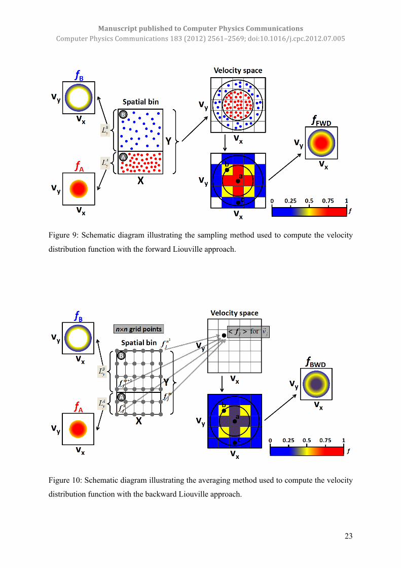
approach. In order to better understand the differences between the two, a schematic

representation is shown in Figures 9 and 10.

Let us consider the problem of calculating the velocity distribution function for a

spatial bin which is localized in a region from the configuration space characterized by a

steep spatial variation of f along Oy direction. The velocity distribution function is

computed using both forward and backward approaches; for the latter approach, the

averaging method is used. We divide the spatial bin in two areas, A and B, characterized by


10

two distinct velocity distribution functions, as shown in Fig. 9 and 10. In area A the velocity

distribution function is the inner core of a Maxwellian distribution function, fA, while in area

B we retrieve the outer shell of the same Maxwellian distribution, fB.

For simplicity, let us assume that f does not vary significantly in either A or B. By

using the forward approach, the particles localized in the both areas A and B will have the

velocities distributed according to their respective velocity distribution functions. Thus, the

less energetic particles will be found in area A, while the most energetic ones will be found in

area B (see Fig. 9). This simplified model corresponds roughly to our simulation results. All

particles localized inside the entire spatial bin will be distributed in velocity space as follows.

Particles originating from area A, i.e. the less energetic ones, will be found in the central

regions of velocity space, while particles originating from area B, i.e. the most energetic

ones, will be found in the outer regions of velocity space.

In order to reconstruct the velocity distribution function by using the forward

approach, a uniform grid in velocity space is defined. For each velocity bin j centred in !v j ,

the corresponding distribution function fFWD(!v j ) is computed by averaging over all

numerical values ijf “attached” to each particle i localized inside the considered velocity bin:

fFWD(!v j ) =

f ji(!v j

i )i=1

nj

∑nj

(9)

where !v j

i is the velocity of particle i localized inside the velocity bin j and jn is the total

number of particles inside bin j. Among these jn particles, let Ajn be the ones from area A

and Bjn those from area B such that A B

j j jn n n= + . Thus, Eq. (9) becomes:

fFWD(!v j ) =

f jiA (!v j

iA )iA=1

njA

∑ + f jiB (!v j

iB )iB=1

njB

∑nj

(10)

where f j

iA (!v jiA) = fA(!v j

iA) , since all Ai particles are localized inside area A and likewise

f j

iB (!v jiB ) = fB(!v j

iB ) , as all Bi particles belongs to area B. Furthermore, we consider that all

velocity bins are small enough such that fA(!v j

iA) = fA(!v j ) and fB(!v j

iB ) = fB(!v j ) . In this way,

f computed using the forward approach for the velocity bin centred on !v j is:


11

fFWD(!v j ) =

njA

nj

fA(!v j )+ 1−nj

A

nj

⎛

⎝⎜

⎞

⎠⎟ fB(!v j ) (11)

In order to compute the velocity distribution function using the backward approach,

we define a uniform grid in configuration space having n×n points that cover the entire area

of the spatial bin to be sampled (see Fig. 10). For each velocity vertex j centred in !v j , the

corresponding distribution function fBWD(!v j ) is computed by averaging over all numerical

values ijf “attached” to each point i of the spatial grid:

fBWD(!v j ) =

f ji(!v j )

i=1

n2

∑n2 (12)

Considering that m grid points are localized inside area A, while the other n2−m grid points

are localized inside area B, Eq. (12) becomes:

fBWD(!v j ) =

f jiA (!v j )

iA=1

m

∑ + f jiB (!v j )

iB=m+1

n2

∑n2 (13)

where f j

iA (!v j ) = fA(!v j ) , since all Ai grid points are localized inside area A, and similarly

f j

iB (!v j ) = fB(!v j ) . Therefore, f computed using the backward approach for the velocity bin

centred on !v j is given by:

fBWD(!v j ) =

mn2 fA(!v j )+ 1− m

n2

⎛⎝⎜

⎞⎠⎟

fB(!v j ) (14)

We should mention that the average value (14) has been obtained simply by computing the

arithmetic mean of all n2 function’s values instead of integrating the velocity distribution

function over the entire spatial bin using a 2D trapezoidal integration rule, as it is done in our

simulations. Also, we considered a uniform grid in velocity space for the backward approach,

while in our simulations an unstructured grid has been used to compute the velocity

distribution function. These simplifications should not have major consequences on the final

results.

In order to compare the velocity distribution functions obtained from both forward

and backward approaches we considered three representative velocity bins, designated a, b

and c and centred at !va , !vb and

!vc (see Fig. 9 and Fig. 10), to compute the numerical values

of f given by Eq. (11) and Eq. (14). These three velocity bins have been chosen such that:


12

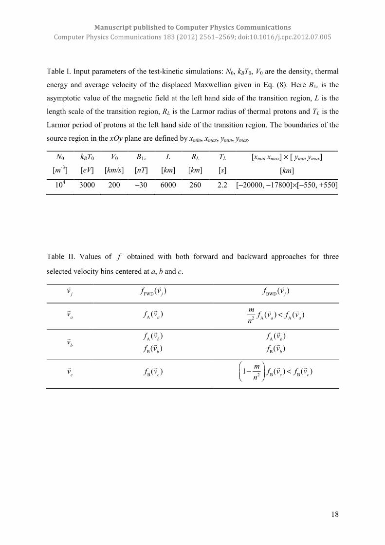
fA(!va ) ≠ 0 and fB(!va ) = 0 , fA(!vb ) = fB(!vb ) ≠ 0 , while fA(!vc ) = 0 and fB(!vc ) ≠ 0 .

Therefore, from Eq. (11) and Eq. (14), we obtain the values of f computed with both

forward and backward approaches for velocity bins a, b and c. The results are given in Table

II and show that the velocity distribution function given by the backward approach is smaller

than the one obtained from the forward approach for velocity bins a and c, while for bin b

both values are equal.

By applying this algorithm to all velocity space bins, a Maxwellian distribution

function is obtained with the forward approach, as can be seen in Fig. 9. However, f

obtained with the backward approach presents a cavity in the central region of velocity space,

as can be seen in Fig. 10. Similar results are obtained, for instance, for bin C2 of our

simulations depicted in Fig. 6 and Fig. 8, which is localized in a region characterized by a

steep spatial variation of the velocity distribution function. Indeed, with the forward approach

a Maxwellian distribution is obtained for bin C2, while with the backward approach the

distribution function is characterized by a central cavity in velocity space. Thus, the

simplified model described in Fig. 9 and Fig. 10 explains the differences obtained between

forward and backward approaches in spatial regions characterized by sharp gradients of f .

The velocity distribution functions given by Eq. (11), for the forward approach, and

Eq. (14), for the backward approach, have similar mathematical expressions except for the

weight coefficients of fA and fB. In the forward approach the weight coefficients are expressed

in terms of /Aj jn n , i.e. the ratio of the number of particles localized inside velocity bin j and

pertaining to spatial area A to the total number of particles localized inside velocity bin j. In

the backward approach the weight coefficients are expressed in terms of 2/m n , i.e. the ratio

of grid points number localized inside area A to total number of grid points localized inside

the entire spatial bin. By analyzing the /Aj jn n ratio we can conclude that this quantity

depends on the position of bin j in velocity space. On the other hand, 2/m n is equal to the

ratio of region A area to entire spatial bin area, which is independent on the position of bin j

in velocity space:

2

( )( )

Ay

y

Lm Area An Area bin L

= = (15)

where AyL indicates the width of area A along the y-axis, while yL represent the width of the

entire spatial bin. Thus, the weight coefficients corresponding to forward and backward

distribution functions are not equal in general and the results provided by the two approaches


13

may also be different, independently of the number of particles injected in the forward

simulations or the number of grid points used in the averaging scheme for the backward

simulations.

The main point which distinguishes the averaging method (14) from the sampling

method (11) is related to the fact that, in the backward approach, to a given point in velocity

space correspond n2 points in the configuration space which cover the entire area of the

spatial bin. In the forward approach however, a given bin in velocity space may originate

from only a subset of points in configuration space localized in a certain area of the spatial

bin. Therefore, in order to calculate the numerical value of the distribution function at a

certain bin in velocity space, the backward averaging method (14) will take into account the

contribution from the entire spatial bin, while the forward sampling method (11) will take

into account the contribution of only a part of the considered spatial bin, thus possibly leading

to different results. Nevertheless, FWDf given by Eq. (11) would be equal to BWDf given by

Eq. (14) if 2m n= . This condition is satisfied if we increase the size of region A such that it

will cover the entire area of the spatial bin. Only in this case Ajn will also be equal to jn for

all velocity space bins and the weight coefficients corresponding to forward and backward

distribution functions will be equal. Therefore, by increasing the size of area A it is possible

to obtain converging results with both approaches as long as the initial assumption is

satisfied, i.e. there are no significant spatial variations of f along area A. We should note

that this assumption will always be satisfied for region B since the size of this area

continually decreases, as the size of A increases. This result can be generalized for three-

dimensional bins with spatial variations of the velocity distribution function along all three

coordinate axes. In this case the forward and backward approaches will return similar results

only for those spatial bins which are small enough such that the following inequality to be

satisfied simultaneously along all three coordinates axes:

ii

fL fx∂⋅ <<∂

(16)

where i = 1, 2, 3 for the x, y, z axes respectively. On the other hand, with bins covering

regions of configuration space characterized by sharp spatial gradients of the velocity

distribution function, the forward and backward approaches will generally provide different

results.


14

4. Conclusions

In this paper we performed a comparative study of the forward and backward

Liouville approaches corresponding to the test-kinetic simulation method that integrates

numerically test-particle orbits in given electric and magnetic fields. The test-kinetic method

has been applied to study various problems of space plasma physics. In this paper we discuss

an example relevant for magnetospheric physics that is analyzed in detail in a previous

publication [21]. The test-kinetic method is an important simulation tool, especially in

complex situations where the use of fully self-consistent kinetic methods is not possible. We

applied the forward and backward approaches to compute the velocity distribution function in

different areas of a proton cloud moving in the vicinity of a region with a sharp transition of

the magnetic field and a non-uniform electric field. The source region is localized in the left

hand side of the transition region and it is characterized by a displaced Maxwellian

distribution function.

We compare the velocity distribution functions obtained for different regions of the

proton cloud with the forward and backward approaches. In the forward approach f is

sampled over a spatial bin which needs to be populated by a sufficiently large number of

particles so as to reduce statistical errors. On the other hand, in the backward approach f is

computed without statistical errors, at precise positions in configuration space. In order to

compare the distribution functions obtained with both approaches, a spatial averaging of f is

needed. The velocity distribution function given by the backward approach is numerically

integrated over a rectangular domain corresponding to the spatial bin used to compute the

distribution function with the forward approach.

Our simulation results show that there are significant differences between the

distribution functions given by forward and backward approaches. The differences are

observed especially for spatial bins from regions with a steep spatial variation of the velocity

distribution function, while in regions with smooth variations of f the two approaches

provide similar results. The differences and similarities can be explained by a careful

examination of the sampling method used in the forward approach and the averaging method

used in the backward approach. The main difference between the two computational methods

is due to the approach used to estimate the velocity distribution function in a spatial bin: the

backward method uses an averaging method that takes into account the contribution of the

entire spatial bin to calculate the distribution function for a certain bin in velocity space,

while, in certain cases, the forward sampling method effectively only takes into account the


15

contribution from a part of the bin considered. The two approaches lead to similar results

when averages are calculated over bins in which the distribution function varies smoothly in

configuration space.

Acknowledgements

This paper is supported by the Sectoral Operational Programme Human Resources

Development (SOP HRD) financed from the European Social Fund and by the Romanian

Government under Contract No. SOP HRD/107/1.5/S/82514. Marius Echim and Gabriel

Voitcu acknowledge support from the European Space Agency (ESA) through PECS Project

no. 98049/2007 − KEEV and thanks International Space Science Institute in Bern,

Switzerland for supporting the team “Plasma entry and transport in the plasma sheet” led by

Simon Wing. Richard Marchand was supported by the Natural Sciences and Engineering

Research Council of Canada.


16

References

[1] R. Marchand, Test-particle simulation of space plasma, Commun. Comput. Phys. 8,

(2010) 471 – 483.

[2] J. S. Wagner, J. R. Kan, S.-I. Akasofu, Particle dynamics in the plasma sheet, J.

Geophys. Res. 84 (1979) 891 – 897.

[3] T. W. Speiser, D. J. Williams, H. A. Garcia, Magnetospherically trapped ions as a source

of magnetosheath energetic ions, J. Geophys. Res. 86 (1981) 723 – 732.

[4] D. B. Curran, C. K. Goertz, T. A. Whelan, Ion Distributions in a Two-Dimensional

Reconnection Field Geometry, Geophys. Res. Lett. 14 (1987) 99 – 102.

[5] D. B. Curran, C. K. Goertz, Particle Distributions in a Two-Dimensional Reconnection

Field Geometry, J. Geophys. Res. 94 (1989) 272 – 286.

[6] M. Ashour-Abdalla, L. M. Zelenyi, V. Peroomian, R. L. Richard, Consequences of

magnetotail ion dynamics, J. Geophys. Res. 99 (1994 )14891 – 14916.

[7] R. L. Richard, R. J.Walker, M. Ashour-Abdalla, The population of the magnetosphere

by solar winds ions when the interplanetary magnetic field is northward, Geophys. Res.

Lett. 21 (1994) 2455–2458.

[8] P. L. Rothwell, M. B. Silevitch, L. P. Block, C.-G. Fälthammar, Particle dynamics in a

spatially varying electric field, J. Geophys. Res. 100 (1995) 14875 – 14885.

[9] D. C. Delcourt, R. F. Jr. Martin, F. Alem, A simple model of magnetic moment

scattering in a field reversal, Geophys. Res. Lett. 21 (1994) 1543 – 1546.

[10] D. C. Delcourt, J. A. Sauvaud, R. F. Jr. Martin, T. E. Moore, Gyrophase effects in the

centrifugal impulse model of particle motion in the magnetotail, J. Geophys. Res. 100

(1995) 17211 – 17220.

[11] D. C. Delcourt, J. A. Sauvaud, R. F. Jr. Martin, T. E. Moore, On the non-adiabatic

precipitation of ions from the near-Earth plasma sheet, J. Geophys. Res. 101 (1996)

17409 – 17418.

[12] F. Mackay, R. Marchand, K. Kabin, J. Y. Lu, Test kinetic modelling of collisionless

perpendicular shocks, J. Plasma Phys. 74 (2008) 301 – 318.


17

[13] R. Marchand, F. Mackay, J. Y. Lu, K. Kabin, Consistency check of a global MHD

simulation using the test-kinetic approach, Plasma Phys. Control. Fusion, 50 (2008)

074007.

[14] J. L. Delcroix, A. Bers, Physique des plasmas, Savoirs Actuels-InterÉditions/CNRS

Éditions, Paris, 1994.

[15] A. Sestero, Structure of plasma sheaths, Phys. Fluids 7 (1964) 44 – 51.

[16] J. Lemaire, L. F. Burlaga, Diamagnetic boundary layers: a kinetic theory, Astrophys.

Space Sci., 45 (1976) 303 – 325.

[17] M. Roth, J. DeKeyser, M. M. Kuznetsova, Vlasov theory of the equilibrium structure of

tangential discontinuities in space plasmas, Space Science Reviews, 76 (1996) 251 –

317.

[18] M. M. Echim, J. Lemaire, Advances in the kinetic treatment of the solar wind

magnetosphere interaction: the impulsive penetration mechanism , in: P. Newell, T.

Onsager (Eds.), Earth's Low Latitude Boundary Layer, American Geophysical Union,

Washington, 2003, pp. 169 – 179.

[19] G. Schmidt, Plasma motion across magnetic fields, Phys. Fluids 3 (1960) 961 – 965.

[20] M. Galvez, G. Gisler, C. Barnes, Computer simulations of finite plasmas convected

across magnetized plasmas, Phys. Fluids B 2 (1990) 516 – 522.

[21] G. Voitcu, M. M. Echim, Ring-shaped velocity distribution functions in energy-

dispersed structures formed at the boundaries of a proton stream injected into a

transverse magnetic field: Test-kinetic results, Phys. Plasmas 19 (2012) 022903-1 −

022903-13.


18

Table I. Input parameters of the test-kinetic simulations: N0, kBT0, V0 are the density, thermal

energy and average velocity of the displaced Maxwellian given in Eq. (8). Here B1z is the

asymptotic value of the magnetic field at the left hand side of the transition region, L is the

length scale of the transition region, RL is the Larmor radius of thermal protons and TL is the

Larmor period of protons at the left hand side of the transition region. The boundaries of the

source region in the xOy plane are defined by xmin, xmax, ymin, ymax.

N0

[m-3]

kBT0

[eV]

V0

[km/s]

B1z

[nT]

L

[km]

RL

[km]

TL

[s]

[xmin xmax] × [ ymin ymax]

[km]

104 3000 200 −30 6000 260 2.2 [−20000, −17800]×[−550, +550]

Table II. Values of f obtained with both forward and backward approaches for three

selected velocity bins centered at a, b and c.

!v j

fFWD(!v j )

fBWD(!v j )

!va fA (!va )

mn2 fA (!va ) < fA (!va )

!vb

fA (!vb )fB(!vb )

fA (!vb )fB(!vb )

!vc fB(!vc )

1− m

n2

⎛⎝⎜

⎞⎠⎟

fB(!vc ) < fB(!vc )


19

Figure 1: Schematic diagram of the forward Liouville approach; a positive time step is used

to integrate test-particle orbits in given magnetic and electric fields.

Figure 2: Schematic diagram of the backward Liouville approach; a negative time step is used

to integrate test-particle orbits in given magnetic and electric fields.


20

Figure 3: Left panel: magnetic field profile in the simulation domain; the B-field is

unidirectional and changes orientation at x=0. Right panel: electric field profile in the

simulation domain; Ey changes sign whenever Bz reverses sign. The simulation domain is

limited by: −40000 km ≤ x ≤ +40000 km, −30000 km ≤ y ≤ +30000 km.

Figure 4: The left panel shows proton density profile in the xOy plane, perpendicular to the

magnetic field, at t=0. The local number density is color coded using a 2D mesh of 60x60

spatial cells. The right panel shows the velocity distribution function, in the vz=0 cross

section, sampled in the blue rectangle in the left panel. Note that the initial distribution

function is given by a displaced Maxwellian with an average velocity V0=200 km/s along the

x direction.


21

Figure 5: Proton density distribution in the xOy plane, perpendicular to the magnetic field, at

t=225s (∼100⋅TL) obtained with the forward approach. The local number density is color

coded using a 2D mesh of 60x60 spatial cells. The density distribution is elongated in +Oy

direction due to the gradient-B drift acting in the region of non-uniform fields. The blue

rectangles indicate the spatial bins used to sample the velocity distribution function shown in

Fig. 6.

Figure 6: Velocity distribution functions obtained at t=225 s (∼100⋅TL) using the forward

approach in the spatial bins indicated by blue rectangles in Fig. 5. The plots correspond to

vz=0 cross-sections in velocity space.


22

Figure 7: Velocity distribution functions obtained at t=225 s (∼100⋅TL) using the backward

approach for the central points of the bins indicated by blue rectangles in Fig. 5. C1* is the

middle point between C1 and C2. The plots show vz=0 cross-sections in velocity space.

Figure 8: Velocity distribution functions obtained at t=225 s (∼100⋅TL) with the backward

approach by averaging over the spatial bins indicated with blue rectangles in Fig. 5. The plots

show vz=0 cross-sections in velocity space.


23

Figure 9: Schematic diagram illustrating the sampling method used to compute the velocity

distribution function with the forward Liouville approach.

Figure 10: Schematic diagram illustrating the averaging method used to compute the velocity

distribution function with the backward Liouville approach.

comparative study of forward and backward test-kinetic ... · comparative study of forward and...

Documents