comparative analysis of speech compression on 8-bit and 16-bit data using different wavelets

International Journal of Computer Trends and Technology (IJCTT) - volume4 Issue5–May 2013

ISSN: 2231-2803 http://www.ijcttjournal.org 251

Comparative analysis of Speech Compression on 8-bit

and 16-bit data using different wavelets

Vini Malika, Pranjal Singh

b Atul kumar Singh

c, Monika Singh

d

Assistant Professora, Studentb,c,d

Electronics & Communication Department, CET-IILM-AHL College,

Affiliated to Gautam Buddha Technical University

Greater Noida- 201306

Abstract— Audio compression is done in order to minimize the

memory requirements of an audio file. This paper presents a novel

idea to achieve this by reducing the bit rate of a speech signal

without compromising with perceptual quality.LPC coding is the

most preferred technique but it provides the loss of information. By

selecting an efficient technique of wavelet transform, we apply

compression on speech signal using MATLAB software on a core-

2duo processor based computing device. The different families of

wavelet are used in order to extract data such as compression

scores and energy levels of an acoustic signal. The simulation

results are taken with different wavelets on 8-bit and 16-bit signal.

These simulation comparisons would represent the efficiency of a

particular family and thus our aim of less memory consumption by

reducing the bit rate of an audio file without effecting the quality

and integrity of the signal is achieved.

Keywords— Compression score, Energy Level, Bit rate, Matlab,

Wavelet transform

I. INTRODUCTION

This audio compression is achieved in two ways. Either

by compressing the data samples using proper encoding

formats else by dynamic adjustments on the range of the

signal. The former technique is utilized in this paper. Compression can be either lossy or lossless. Lossless

compression reduces bits by identifying and eliminating

statistical redundancy. No information is lost in lossless

compression. The process of reducing the size of a data file is

popularly referred to as data compression which is formally

called Source coding. Lossy method reduces bits by removing

unnecessary information.

A significant advantage of using wavelets for speech

coding is that the compression ratio can easily be varied,

while most other techniques have fixed compression ratios

keeping all the other parameters constant. Wavelet analysis is the breaking up of a signal into a set of scaled and translated

versions of an original (or mother) wavelet [5]. Taking the

wavelet transform of a signal decomposes the original signal

into wavelets coefficients at different scales and positions.

These coefficients represent the signal in the wavelet domain

and all data operations can be performed using just the

corresponding wavelet coefficients [6][7].

The paper is classified as follows: Section II includes

Compression algorithms and techniques which include LPC

compression technique and an overview of wavelet transform.

Section III includes compression technique using different

wavelet and their simulation results. Section IV includes the

comparison of result using the parameter compression score and energy recovery. In is, comparison is also shown by

graphical representation. Section V includes the conclusion

and future scope.

II. COMPRESSION ALGORITHMS AND TECHNIQUES

An Speech signals has unique properties that differ from a

general audio/music signals. First, speech is a signal that is

more structured and band-limited around 4 kHz. These two

facts can be exploited through different models and

approaches and at the end, make it easier to compress. Many

speech compression techniques have been efficiently applied.

The example below shows how a signal is reduced by 2:1 (the

output level above the threshold is halved) and 10:1(severe compression).

Basically speech coders can be classified into two

categories: waveform coders and analysis by synthesis

vocoders. The first was explained before and are not very used

for speech compression, because they do not provide

considerable low bit rates. They are mostly focused to

broadband audio signals. On the other hand, vocoders use an

entirely different approach to speech coding, known as

parametric coding, or analysis by synthesis coding where no

attempt is made at reproducing the exact speech waveform at

the receiver, but to create perceptually equivalent to the signal. These systems provide much lower data rates by using a

functional model of the human speaking mechanism at the

receiver. Among those, perhaps one of the most popular

techniques is called Linear Predictive Coding (LPC) vocoder.


ISSN: 2231-2803 http://www.ijcttjournal.org Page 1252

MPEG audio standards include an elaborate description of

perceptual coding, psychoacoustic modeling and

implementation issues. It is interesting to mention some brief

comments on these audio coders, because some of the features

of the wavelet-based audio coders are based in those models.

MP1 (MPEG audio layer-1): Simplest coder/decoder.

It identifies local tonal components based on local

peaks of the audio spectrum.

MP2 (MPEG audio layer-2): It has an intermediate

complexity. It uses data from the previous two

windows to predict, via linear interpolation, the

component of the current window. This is based on

the fact that tonal components, being more

predictable, have higher tonality indices.

MP3 (MPEG audio layer-3): Higher level of

complexity. Not only includes masking in time

domain but also a more elaborated psychoacoustic

model, MDCT decomposition, dynamic allocation

and Huffman coding.

A. Linear Predictive Coding

Linear predictive coding (LPC) is defined as a digital

method for encoding an analog signal in which a particular

value is predicted by a linear function of the past values of the

signal. Human speech is produced in the vocal tract which can

be approximated as a variable diameter tube. The linear

predictive coding (LPC) model is based on a mathematical

approximation of the vocal tract represented by this tube of a

varying diameter. At a particular time, t, the speech sample s (t) is represented as a linear sum of the p previous samples.

The most important aspect of LPC is the linear predictive

filter which allows the value of the next sample to be

determined by a linear combination of previous samples.

At this reduced rate the speech has a distinctive synthetic

sound and there is a noticeable loss of quality. However, the

speech is still audible and it can still be easily understood.

Since there is information loss in linear predictive coding, it

is a lossy form of compression.

B. Speech Encoding

LPC coding function will take the speech audio signal and

divide it into 30mSec frames. These frames start every

20mSec. Thus each frame overlaps with the previous and next

frame. After the frames have been separated, the LPC function

will take every frame and extract the necessary information

from it. This is the voiced/unvoiced, gain, pitch, and filter

coefficients information.

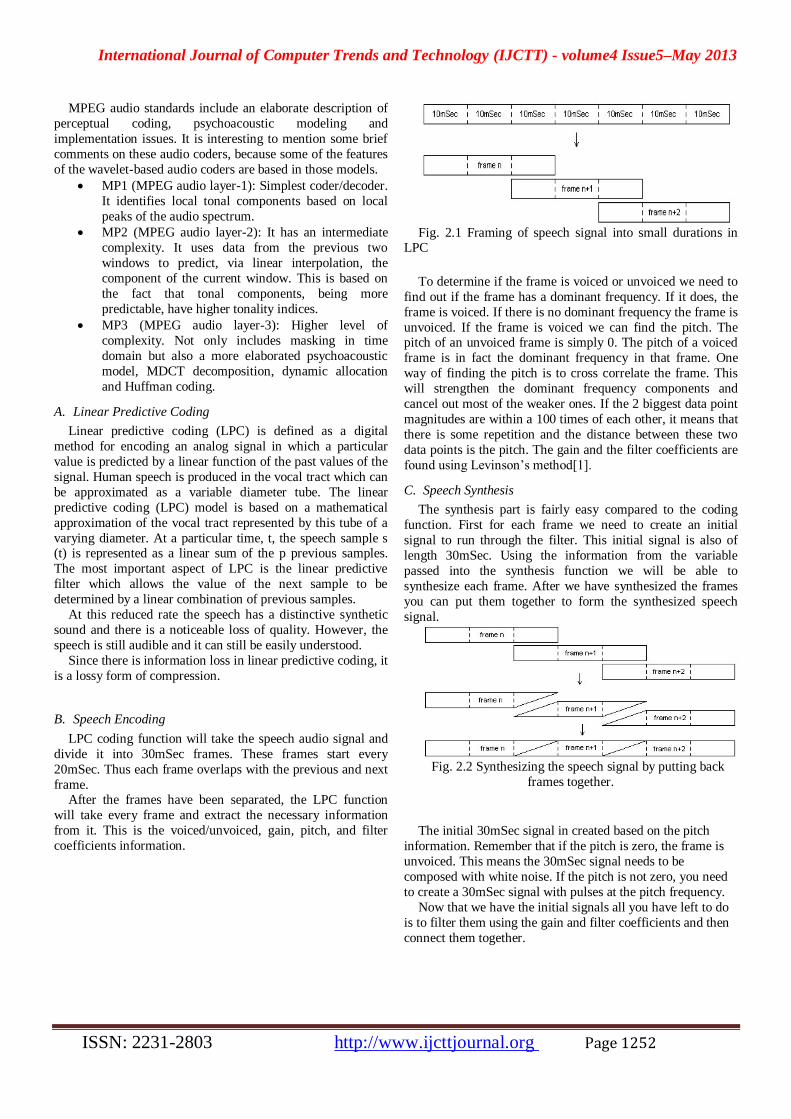
Fig. 2.1 Framing of speech signal into small durations in

LPC To determine if the frame is voiced or unvoiced we need to

find out if the frame has a dominant frequency. If it does, the

frame is voiced. If there is no dominant frequency the frame is

unvoiced. If the frame is voiced we can find the pitch. The pitch of an unvoiced frame is simply 0. The pitch of a voiced

frame is in fact the dominant frequency in that frame. One

way of finding the pitch is to cross correlate the frame. This

will strengthen the dominant frequency components and

cancel out most of the weaker ones. If the 2 biggest data point

magnitudes are within a 100 times of each other, it means that

there is some repetition and the distance between these two

data points is the pitch. The gain and the filter coefficients are

found using Levinson’s method[1].

C. Speech Synthesis

The synthesis part is fairly easy compared to the coding

function. First for each frame we need to create an initial

signal to run through the filter. This initial signal is also of

length 30mSec. Using the information from the variable

passed into the synthesis function we will be able to

synthesize each frame. After we have synthesized the frames

you can put them together to form the synthesized speech

signal.

Fig. 2.2 Synthesizing the speech signal by putting back

frames together.

The initial 30mSec signal in created based on the pitch

information. Remember that if the pitch is zero, the frame is

unvoiced. This means the 30mSec signal needs to be

composed with white noise. If the pitch is not zero, you need

to create a 30mSec signal with pulses at the pitch frequency.

Now that we have the initial signals all you have left to do

is to filter them using the gain and filter coefficients and then

connect them together.



Putting the frames back together is also done in a special

way. This is where the reason for having the frames overlap

becomes clear. Because each frame has its own pitch, gain and

filter, if we simply put them text to each other after

synthesizing them all, it would sound very choppy. By making

them overlap, we can smooth the transition from one frame to

the next. The figure below shows how the frames are

connected. The amplitude of the tip and tail of each frame’s data is scaled and then simply added.

Since there is information loss in linear predictive coding, it

is a lossy form of compression.

MatLab Implementation [7]

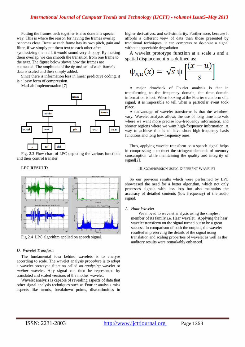
Fig. 2.3 Flow chart of LPC depicting the various functions

and their control transfer

LPC RESULT:

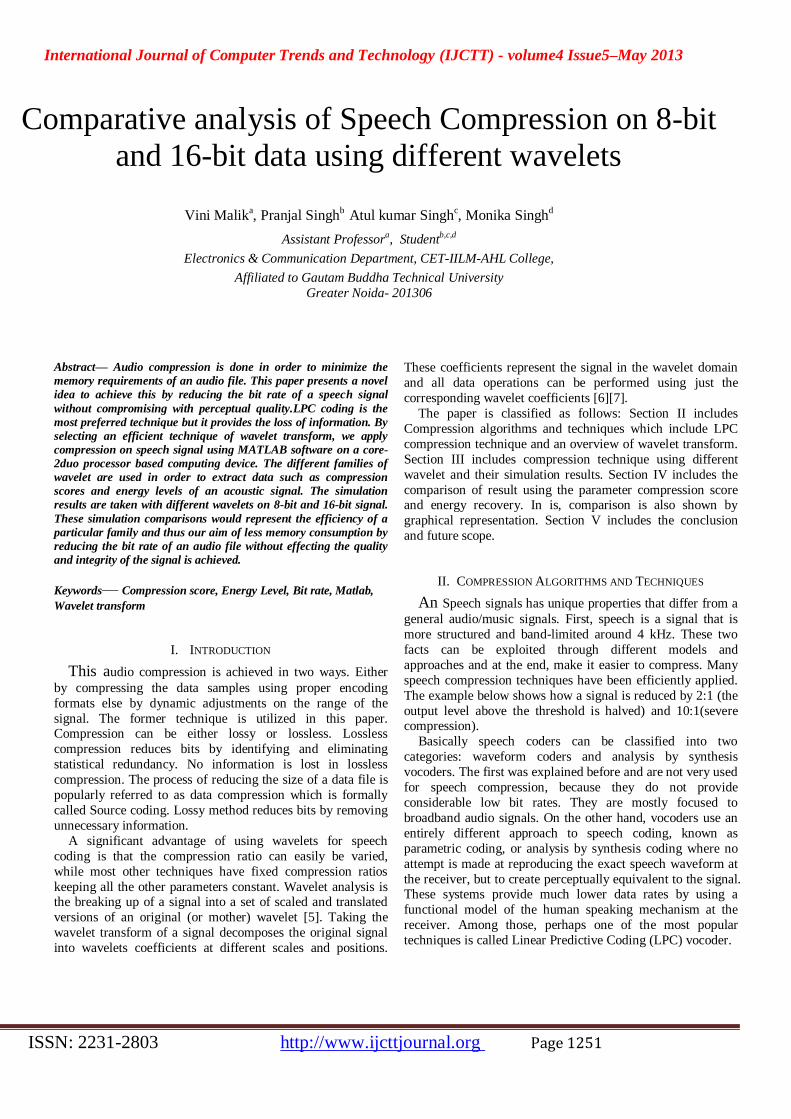
Fig.2.4 LPC algorithm applied on speech signal.

D. Wavelet Transform

The fundamental idea behind wavelets is to analyse according to scale. The wavelet analysis procedure is to adopt

a wavelet prototype function called an analysing wavelet or

mother wavelet. Any signal can then be represented by

translated and scaled versions of the mother wavelet.

Wavelet analysis is capable of revealing aspects of data that

other signal analysis techniques such as Fourier analysis miss

aspects like trends, breakdown points, discontinuities in

higher derivatives, and self-similarity. Furthermore, because it

affords a different view of data than those presented by

traditional techniques, it can compress or de-noise a signal

without appreciable degradation

A wavelet prototype function at a scale s and a

spatial displacement u is defined as:

A major drawback of Fourier analysis is that in

transforming to the frequency domain, the time domain

information is lost. When looking at the Fourier transform of a

signal, it is impossible to tell when a particular event took

place.

An advantage of wavelet transforms is that the windows

vary. Wavelet analysis allows the use of long time intervals

where we want more precise low-frequency information, and

shorter regions where we want high-frequency information. A way to achieve this is to have short high-frequency basis

functions and long low-frequency ones.

Thus, applying wavelet transform on a speech signal helps

in compressing it to meet the stringent demands of memory

consumption while maintaining the quality and integrity of

signal[2].

III. COMPRESSION USING DIFFERENT WAVELET

So our previous results which were performed by LPC

showcased the need for a better algorithm, which not only

processes signals with less loss but also maintains the

accuracy of detailed contents (low frequency) of the audio

signal.

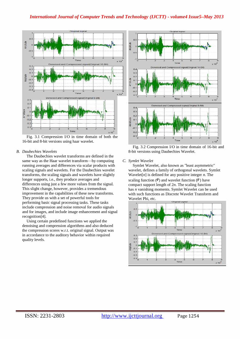
A. Haar Wavelet

We moved to wavelet analysis using the simplest

member of its family i.e. Haar wavelet. Applying the haar

wavelet transform on the signal turned out to be a great

success. In comparison of both the outputs, the wavelet

resulted in preserving the details of the signal using

translation and scaling properties of wavelet as well as the

auditory results were remarkably enhanced.



Fig. 3.1 Compression I/O in time domain of both the

16-bit and 8-bit versions using haar wavelet.

B. Daubechies Wavelets

The Daubechies wavelet transforms are defined in the

same way as the Haar wavelet transform—by computing

running averages and differences via scalar products with

scaling signals and wavelets. For the Daubechies wavelet

transforms, the scaling signals and wavelets have slightly

longer supports, i.e., they produce averages and

differences using just a few more values from the signal.

This slight change, however, provides a tremendous

improvement in the capabilities of these new transforms. They provide us with a set of powerful tools for

performing basic signal processing tasks. These tasks

include compression and noise removal for audio signals

and for images, and include image enhancement and signal

recognition[4].

Using certain predefined functions we applied the

denoising and compression algorithms and also deduced

the compression scores w.r.t. original signal. Output was

in accordance to the auditory behavior within required

quality levels.

Fig. 3.2 Compression I/O in time domain of 16-bit and

8-bit versions using Daubechies Wavelet.

C. Symlet Wavelet Symlet Wavelet, also known as "least asymmetric"

wavelet, defines a family of orthogonal wavelets. Symlet

Wavelet[n] is defined for any positive integer n. The

scaling function ( ) and wavelet function ( ) have compact support length of 2n. The scaling function

has n vanishing moments. Symlet Wavelet can be used

with such functions as Discrete Wavelet Transform and

Wavelet Phi, etc.




8-bit versions using symlet Wavelet.

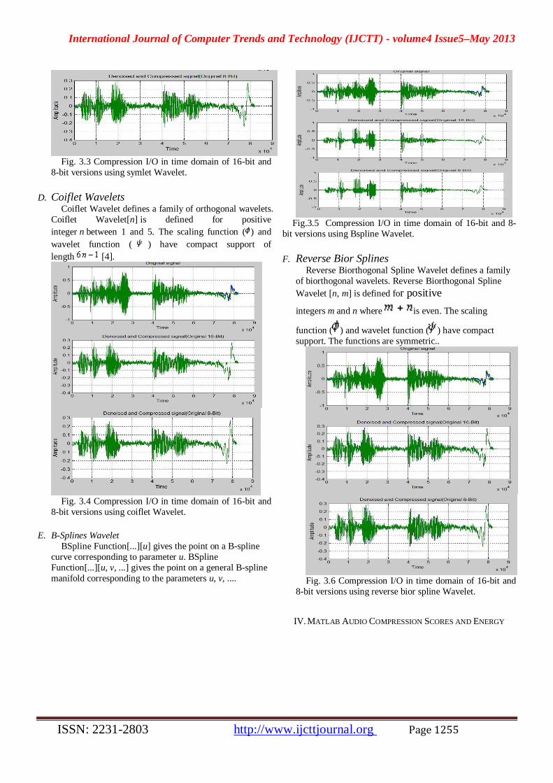
D. Coiflet Wavelets Coiflet Wavelet defines a family of orthogonal wavelets.

Coiflet Wavelet[n] is defined for positive

integer n between 1 and 5. The scaling function ( ) and

wavelet function ( ) have compact support of

length [4].


8-bit versions using coiflet Wavelet.

E. B-Splines Wavelet

BSpline Function[...][u] gives the point on a B-spline

curve corresponding to parameter u. BSpline

Function[...][u, v, ...] gives the point on a general B-spline

manifold corresponding to the parameters u, v, ....

Fig.3.5 Compression I/O in time domain of 16-bit and 8-

bit versions using Bspline Wavelet.

F. Reverse Bior Splines Reverse Biorthogonal Spline Wavelet defines a family

of biorthogonal wavelets. Reverse Biorthogonal Spline Wavelet [n, m] is defined for positive

integers m and n where is even. The scaling

function ( ) and wavelet function ( ) have compact

support. The functions are symmetric..


8-bit versions using reverse bior spline Wavelet.

IV. MATLAB AUDIO COMPRESSION SCORES AND ENERGY



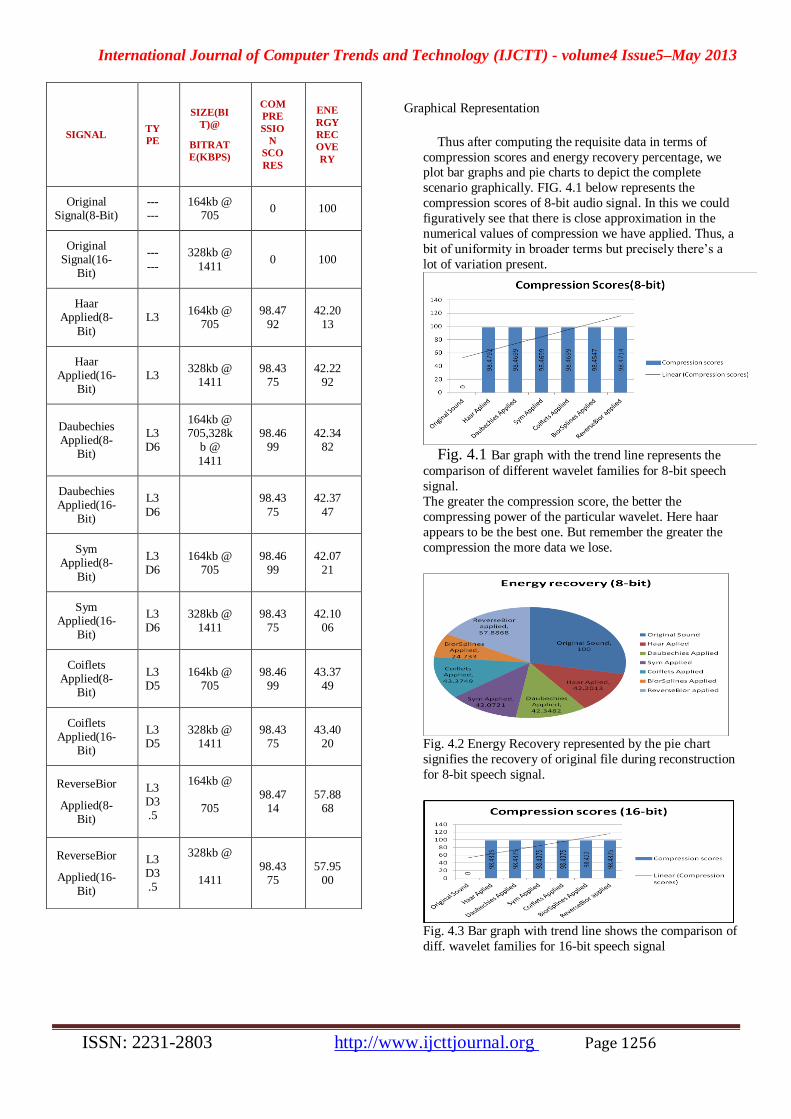
Graphical Representation

Thus after computing the requisite data in terms of

compression scores and energy recovery percentage, we plot bar graphs and pie charts to depict the complete

scenario graphically. FIG. 4.1 below represents the

compression scores of 8-bit audio signal. In this we could

figuratively see that there is close approximation in the

numerical values of compression we have applied. Thus, a

bit of uniformity in broader terms but precisely there’s a

lot of variation present.

Fig. 4.1 Bar graph with the trend line represents the

comparison of different wavelet families for 8-bit speech

signal. The greater the compression score, the better the

compressing power of the particular wavelet. Here haar

appears to be the best one. But remember the greater the

compression the more data we lose.

Fig. 4.2 Energy Recovery represented by the pie chart

signifies the recovery of original file during reconstruction

for 8-bit speech signal.

Fig. 4.3 Bar graph with trend line shows the comparison of

diff. wavelet families for 16-bit speech signal

SIGNAL TY

PE

SIZE(BI

T)@

BITRAT

E(KBPS)

COM

PRE

SSIO

N

SCO

RES

ENE

RGY

REC

OVE

RY

Original Signal(8-Bit)

------

164kb @ 705

0 100

Original Signal(16-

Bit)

---

---

328kb @

1411 0 100

Haar Applied(8-

Bit)

L3 164kb @

705 98.47

92 42.20

13

Haar Applied(16-

Bit) L3

328kb @ 1411

98.4375

42.2292

Daubechies Applied(8-

Bit)

L3D6

164kb @ 705,328k

b @

1411

98.4699

42.3482

Daubechies Applied(16-

Bit)

L3

D6

98.43

75

42.37

47

Sym Applied(8-

Bit)

L3D6

164kb @ 705

98.4699

42.0721

Sym Applied(16-

Bit)

L3D6

328kb @ 1411

98.4375

42.1006

Coiflets Applied(8-

Bit)

L3D5

164kb @ 705

98.4699

43.3749

Coiflets Applied(16-

Bit)

L3D5

328kb @ 1411

98.4375

43.4020

ReverseBior

Applied(8-Bit)

L3D3.5

164kb @

705 98.47

14 57.88

68

ReverseBior

Applied(16-Bit)

L3D3.5

328kb @

1411 98.43

75 57.95

00



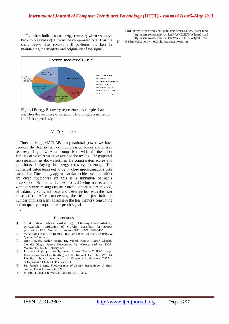
Fig below indicates the energy recovery when we move

back to original signal from the compressed one. This pie

chart shows that reverse still performs the best in

maintaining the integrity and originality of the signal.

Fig. 4.4 Energy Recovery represented by the pie chart

signifies the recovery of original file during reconstruction

for 16-bit speech signal.

V. CONCLUSION

Thus utilizing MATLAB computational power we have

deduced the data in terms of compression scores and energy

recovery diagrams. After comparison with all the other

families of wavelet we have attained the results. The graphical representation as shown notifies the compression scores and

pie charts displaying the energy recovery percentage. The

numerical value turns out to be in close approximations with

each other. Thus it may appear that daubechies, symlet, coiflet

are close contenders yet this is a limitation of one’s

observation. Symlet is the best for achieving bit reduction

without compromising quality. Since auditory nature is good,

r/l balancing sufficient, bass and treble perfect with the least

noise effect. After compressing the 16-bit, just half the

number of bits present, to achieve the less memory consuming

and no quality compromised speech signal.

.

REFERENCES

[1] S. M. Subhra Debdas, Vaishali Jagrit, Chinmay Chandrashekhar,

M.F.Qureshi. Application of Wavelet Transform for Speech

processing .IJEST: Vol. 3 No. 8 August 2011, ISSN: 0975-5462.

[2] V. Balakrishnan, Nash Borges, Luke Parchment. Wavelet Denoising &

Speech Enhancement.

[3] Nitin Trivedi, Sachin Ahuja, Dr. Vikesh Kumar, Raman Chadha,

Saurabh Singh. Speech Recognition by Wavelet analysis. IJCA:

Volume 15– No.8, February 2011.

[4] Priyanka singh, priti singh, rakesh kumar Sharma,” JPEG Image

Compression based on Biorthogonal, Coiflets and Daubechies Wavelet

Families ” International Journal of Computer Applications (0975 –

8887)Volume 13– No.1, January 2011

[5] Dr. Joseph Picone. Fundamentals of Speech Recognition: A short

course. Texas Instruments,1996.

[6] M. Robi Polikar.The Wavelet Tutorial part: 1, 2, 3.

Link: http://users.rowan.edu/~polikar/WAVELETS/WTpart1.html

http://users.rowan.edu/~polikar/WAVELETS/WTpart2.html

http://users.rowan.edu/~polikar/WAVELETS/WTpart3.htm

[7] R Mathworks home site.Link: http://mathworks.in

comparative analysis of speech compression on 8-bit and 16-bit data using different wavelets

Documents