comparative analysis of machine learning … learning techniques for detecting insurance ... the...
TRANSCRIPT

www.wipro.com
COMPARATIVE ANALYSIS OF MACHINE LEARNING TECHNIQUES FOR DETECTING INSURANCE CLAIMS FRAUD
08 ................................................................................................................................ Model Building and Comparison
15 ................................................................................................................................ Model Verdict
16 ................................................................................................................................ Conclusion
16 ................................................................................................................................ Acknowledgements
17 ................................................................................................................................ Other References
18 ................................................................................................................................ About the Authors
Contents
03 ................................................................................................................................ Abstract
03 ................................................................................................................................ Introduction
04 ................................................................................................................................ Why Machine Learning in Fraud Detection?
04 ................................................................................................................................ Exercise Objectives
05 ................................................................................................................................ Dataset Description
07 ................................................................................................................................ Feature Engineering and Selection

03
Abstract
Insurance fraud detection is a challenging problem, given the variety of fraud patterns and relatively small ratio of known frauds in typical samples. While building detection models, the savings from loss prevention needs to be balanced with cost of false alerts. Machine learning techniques allow for improving predictive accuracy, enabling loss control units to achieve higher coverage with low false positive rates. In this paper, multiple machine learning techniques for fraud detection are presented and their performance on various data sets examined. The impact of feature engineering, feature selection and parameter tweaking are explored with the objective of achieving superior predictive performance.
1.0 Introduction
Insurance frauds cover the range of improper activities which an
individual may commit in order to achieve a favorable outcome from
the insurance company. This could range from staging the incident,
misrepresenting the situation including the relevant actors and the
cause of incident and �nally the extent of damage caused.
Potential situations could include:
Covering-up for a situation that wasn’t covered under insurance
(e.g. drunk driving, performing risky acts, illegal activities etc.)
Misrepresenting the context of the incident: This could include
transferring the blame to incidents where the insured party is to
blame, failure to take agreed upon safety measures
In�ating the impact of the incident: Increasing the estimate of loss
incurred either through addition of unrelated losses (faking losses)
or attributing increased cost to the losses
The insurance industry has grappled with the challenge of insurance
claim fraud from the very start. On one hand, there is the challenge of
impact to customer satisfaction through delayed payouts or prolonged
investigation during a period of stress. Additionally, there are costs of
investigation and pressure from insurance industry regulators. On the
other hand, improper payouts cause a hit to pro�tability and
encourage similar delinquent behavior from other policy holders.
According to FBI, the insurance industry in the USA consists of over
7000 companies that collectively received over $1 trillion annually in
premiums. FBI also estimates the total cost of insurance fraud
(non-health insurance) to be more than $40 billion annually [1].
It must be noted that insurance fraud is not a victimless crime – the
losses due to frauds, impact all the involved parties through increased
premium costs, trust de�cit during the claims process and impacts to
process ef�ciency and innovation.
Hence the insurance industry has an urgent need to develop capability
that can help identify potential frauds with a high degree of accuracy, so
that other claims can be cleared rapidly while identi�ed cases can be
scrutinized in detail.
[1] Source: https://www.fbi.gov/stats-services/publications/insurance-fraud

04
Insurance frauds cover the range of improper activities which an
individual may commit in order to achieve a favorable outcome from
the insurance company. This could range from staging the incident,
misrepresenting the situation including the relevant actors and the
cause of incident and �nally the extent of damage caused.
Potential situations could include:
Covering-up for a situation that wasn’t covered under insurance
(e.g. drunk driving, performing risky acts, illegal activities etc.)
Misrepresenting the context of the incident: This could include
transferring the blame to incidents where the insured party is to
blame, failure to take agreed upon safety measures
In�ating the impact of the incident: Increasing the estimate of loss
incurred either through addition of unrelated losses (faking losses)
or attributing increased cost to the losses
The insurance industry has grappled with the challenge of insurance
claim fraud from the very start. On one hand, there is the challenge of
impact to customer satisfaction through delayed payouts or prolonged
investigation during a period of stress. Additionally, there are costs of
investigation and pressure from insurance industry regulators. On the
other hand, improper payouts cause a hit to pro�tability and
encourage similar delinquent behavior from other policy holders.
According to FBI, the insurance industry in the USA consists of over
7000 companies that collectively received over $1 trillion annually in
premiums. FBI also estimates the total cost of insurance fraud
(non-health insurance) to be more than $40 billion annually [1].
It must be noted that insurance fraud is not a victimless crime – the
losses due to frauds, impact all the involved parties through increased
premium costs, trust de�cit during the claims process and impacts to
process ef�ciency and innovation.
Hence the insurance industry has an urgent need to develop capability
2.0 Why Machine Learning in Fraud Detection?
The traditional approach for fraud detection is based on developing
heuristics around fraud indicators. Based on these heuristics, a decision
on fraud would be made in one of two ways. In certain scenarios rules
would be framed that would de�ne if the case needs to be sent for
investigation. In other cases, a checklist would be prepared with scores
for the various indicators of fraud. An aggregation of these scores along
with the value of the claim would determine if the case needs to be
sent for investigation. The criteria for determining indicators and the
thresholds will be tested statistically and periodically recalibrated.
The challenge with the above approaches is that they rely very heavily
on manual intervention which will lead to the following limitations
Constrained to operate with a limited set of known parameters
based on heuristic knowledge – while being aware that some of the
other attributes could also in�uence decisions
Inability to understand context-speci�c relationships between
parameters (geography, customer segment, insurance sales process)
that might not re�ect the typical picture. Consultations with
that can help identify potential frauds with a high degree of accuracy, so
that other claims can be cleared rapidly while identi�ed cases can be
scrutinized in detail.
industry experts indicate that there is no ‘typical model’, and hence
challenges to determine the model speci�c to context
Recalibration of model is a manual exercise that has to be
conducted periodically to re�ect changing behavior and to ensure
that the model adapts to feedback from investigations. The ability to
conduct this calibration is challenging
Incidence of fraud (as a percentage of the overall claims) is low-
typically less than 1% of the claims are classi�ed. Additionally new
modus operandi for fraud needs to be uncovered on a
proactive basis
These are challenging from a traditional statistics perspective. Hence,
insurers have started looking at leveraging machine learning capability. The
intent is to present a variety of data to the algorithm without judgement
around the relevance of the data elements. Based on identi�ed frauds, the
intent is for the machine to develop a model that can be tested on these
known frauds through a variety of algorithmic techniques.
3.0 Exercise Objectives
Explore various machine learning techniques to improve accuracy of
detection in imbalanced samples. The impact of feature engineering,
feature selection and parameter tweaking are explored with objective
of achieving superior predictive performance.
As a procedure, the data will be split into three different segments –
training, testing and cross-validation. The algorithm will be trained on a
partial set of data and parameters tweaked on a testing set. This will be
examined for performance on the cross-validation set. The
high-performing models will be then tested for various random splits of
data to ensure consistency in results.
The exercise was conducted on ApolloTM – Wipro’s Anomaly
Detection Platform, which applies a combination of pre-de�ned rules
and predictive machine learning algorithms to identify outliers in data.
It is built on Open Source with a library of pre-built algorithms that
enable rapid deployment, and can be customized and managed. This
Big Data Platform is comprised of three layers as indicated below.
Figure 1: Three layers of Apollo’s architecture
DATA HANDLING
DETECTION LAYER OUTCOMES
Data Clensing
Transformation
Tokenizing
Dashboards
Detailed Reports
Case Management
Business Rules
ML Algorithims

24
05
The exercise described above was performed on four different insurance datasets. The names cannot be declared, given reasons of con�dentiality.
Data descriptions for the datasets are given below.
4.0 Data Set Description
All datasets pertain to claims from a single area and relate to motor/
vehicle insurance claims. In all the datasets, a small proportion of claims
are marked as known frauds and others as normal. It is expected that
certain claims marked as normal might also be fraudulent, but these
suspicions were not followed through for multiple reasons (time delays,
late detection, constraints of bandwidth, low value etc.)
The table below presents the feature descriptions
Dataset - 1
8,627
34
12
8,537
90
1.04%
11.36%
10
562,275
59
11
591,902
373
0.06%
10.27%
12
595,360
62
13
595,141
219
0.03%
10.27%
13
15,420
34
14,497
913
5.93%
0.00%
3
Number of Claims
Number of Attributes
Categorical Attributes
Normal Claims
Frauds Identi�ed
Fraud Incidence Rate
Missing Values
Number of Years of Data
Dataset - 2 Dataset - 3 Dataset - 4
Table 1: Features of various datasets
4.I Introduction to Datasets
The insurance dataset can be classi�ed into different categories of
details like policy details, claim details, party details, vehicle details,
repair details, risk details. Some attributes that are listed in the datasets
are: categorical attributes with names: Vehicle Style, Gender, Marital
Status, License Type, and Injury Type etc. Date attributes with names:
Loss Date, Claim Date, and Police Noti�ed Date etc. Numerical
attributes with names: Repair Amount, Sum Insured, Market Value etc.
For better data exploration, the data is divided and explored based on
the perspectives of both the insured party and the third party. After
doing some Exploratory Data Analysis (EDA) on all the datasets, some
key insights are listed below.
Dataset – 1:
Out of all fraudulent claims, 20% of them have involvement with
multiple parties and when a multiple party is involved there is a
4.2 Detailed Description of Datasets
Overall Features:
73% of chance to perform a fraud
11% of the fraudulent claims occurred on holiday weeks. And also
when an accident happens on holiday week it is 80% more likely to
be a fraud
Dataset – 2:
For Insured:
72% of the claimants’ vehicles drivability status is unknown whereas
in non-fraud claims; most of the vehicles have a drivability status as
yes or no
75% of the claimants have their license type as blank which is
suspicious because the non-fraud claims have their license
types mentioned
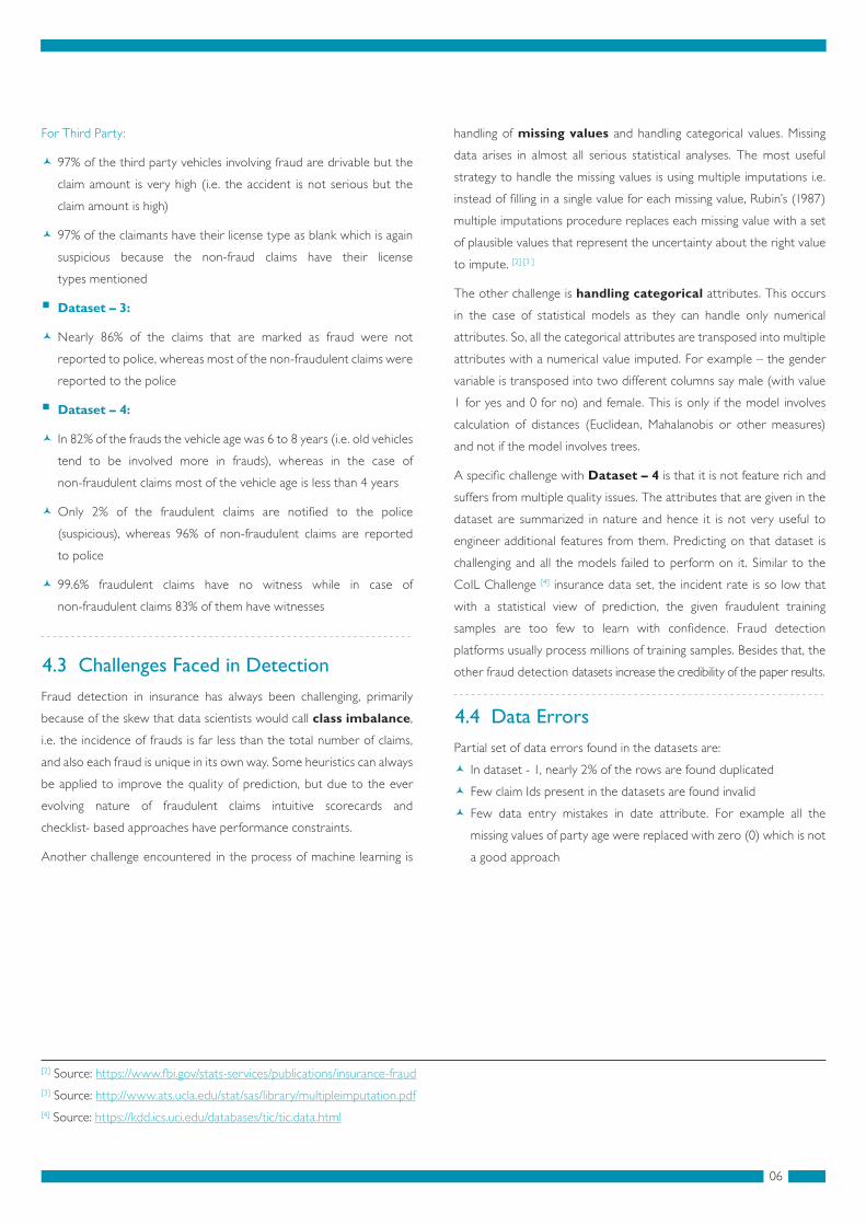
For Third Party:
97% of the third party vehicles involving fraud are drivable but the
claim amount is very high (i.e. the accident is not serious but the
claim amount is high)
97% of the claimants have their license type as blank which is again
suspicious because the non-fraud claims have their license
types mentioned
Dataset – 3:
Nearly 86% of the claims that are marked as fraud were not
reported to police, whereas most of the non-fraudulent claims were
reported to the police
Dataset – 4:
In 82% of the frauds the vehicle age was 6 to 8 years (i.e. old vehicles
tend to be involved more in frauds), whereas in the case of
non-fraudulent claims most of the vehicle age is less than 4 years
Only 2% of the fraudulent claims are noti�ed to the police
(suspicious), whereas 96% of non-fraudulent claims are reported
to police
99.6% fraudulent claims have no witness while in case of
non-fraudulent claims 83% of them have witnesses
06
The insurance dataset can be classi�ed into different categories of
details like policy details, claim details, party details, vehicle details,
repair details, risk details. Some attributes that are listed in the datasets
are: categorical attributes with names: Vehicle Style, Gender, Marital
Status, License Type, and Injury Type etc. Date attributes with names:
Loss Date, Claim Date, and Police Noti�ed Date etc. Numerical
attributes with names: Repair Amount, Sum Insured, Market Value etc.
For better data exploration, the data is divided and explored based on
the perspectives of both the insured party and the third party. After
doing some Exploratory Data Analysis (EDA) on all the datasets, some
key insights are listed below.
Dataset – 1:
Out of all fraudulent claims, 20% of them have involvement with
multiple parties and when a multiple party is involved there is a
Fraud detection in insurance has always been challenging, primarily
because of the skew that data scientists would call class imbalance,
i.e. the incidence of frauds is far less than the total number of claims,
and also each fraud is unique in its own way. Some heuristics can always
be applied to improve the quality of prediction, but due to the ever
evolving nature of fraudulent claims intuitive scorecards and
checklist- based approaches have performance constraints.
Another challenge encountered in the process of machine learning is
4.3 Challenges Faced in Detection
Partial set of data errors found in the datasets are:
In dataset - 1, nearly 2% of the rows are found duplicated
Few claim Ids present in the datasets are found invalid
Few data entry mistakes in date attribute. For example all the
missing values of party age were replaced with zero (0) which is not
a good approach
4.4 Data Errors
handling of missing values and handling categorical values. Missing
data arises in almost all serious statistical analyses. The most useful
strategy to handle the missing values is using multiple imputations i.e.
instead of �lling in a single value for each missing value, Rubin’s (1987)
multiple imputations procedure replaces each missing value with a set
of plausible values that represent the uncertainty about the right value
to impute. [2] [3 ]
The other challenge is handling categorical attributes. This occurs
in the case of statistical models as they can handle only numerical
attributes. So, all the categorical attributes are transposed into multiple
attributes with a numerical value imputed. For example – the gender
variable is transposed into two different columns say male (with value
1 for yes and 0 for no) and female. This is only if the model involves
calculation of distances (Euclidean, Mahalanobis or other measures)
and not if the model involves trees.
A speci�c challenge with Dataset – 4 is that it is not feature rich and
suffers from multiple quality issues. The attributes that are given in the
dataset are summarized in nature and hence it is not very useful to
engineer additional features from them. Predicting on that dataset is
challenging and all the models failed to perform on it. Similar to the
CoIL Challenge [4] insurance data set, the incident rate is so low that
with a statistical view of prediction, the given fraudulent training
samples are too few to learn with con�dence. Fraud detection
platforms usually process millions of training samples. Besides that, the
other fraud detection datasets increase the credibility of the paper results.
[2] Source: https://www.fbi.gov/stats-services/publications/insurance-fraud[3] Source: http://www.ats.ucla.edu/stat/sas/library/multipleimputation.pdf[4] Source: https://kdd.ics.uci.edu/databases/tic/tic.data.html
73% of chance to perform a fraud
11% of the fraudulent claims occurred on holiday weeks. And also
when an accident happens on holiday week it is 80% more likely to
be a fraud
Dataset – 2:
For Insured:
72% of the claimants’ vehicles drivability status is unknown whereas
in non-fraud claims; most of the vehicles have a drivability status as
yes or no
75% of the claimants have their license type as blank which is
suspicious because the non-fraud claims have their license
types mentioned
For Third Party:
97% of the third party vehicles involving fraud are drivable but the
claim amount is very high (i.e. the accident is not serious but the
claim amount is high)
97% of the claimants have their license type as blank which is again
suspicious because the non-fraud claims have their license
types mentioned
Dataset – 3:
Nearly 86% of the claims that are marked as fraud were not
reported to police, whereas most of the non-fraudulent claims were
reported to the police
Dataset – 4:
In 82% of the frauds the vehicle age was 6 to 8 years (i.e. old vehicles
tend to be involved more in frauds), whereas in the case of
non-fraudulent claims most of the vehicle age is less than 4 years
Only 2% of the fraudulent claims are noti�ed to the police
(suspicious), whereas 96% of non-fraudulent claims are reported
to police
99.6% fraudulent claims have no witness while in case of
non-fraudulent claims 83% of them have witnesses

07
5.0 Feature Engineering and Selection
Success in machine learning algorithms is dependent on how the data
is represented. Feature engineering is a process of transforming raw
data into features that better represent the underlying problem to the
predictive models, resulting in improved model performance on
unseen data. Domain knowledge is critical in identifying which features
might be relevant and the exercise calls for close interaction between
a loss claims specialist and a data scientist.
The process of feature engineering is iterative as indicated in the
�gure below
Out of all the attributes listed in the dataset, the attributes that are
relevant to the domain and result in the boosting of model
performance are picked and used. i.e. the attributes that result in the
degradation of model performance are removed. This entire process is
called Feature Selection or Feature Elimination.
Feature selection generally acts as �ltering by opting out features that
reduce model performance.
Wrapper methods are a feature selection process in which different
feature combinations are elected and evaluated using a predictive
model. The combination of features selected is sent as input to the
machine learning model and trained as the �nal model.
Forward Selection: Beginning with zero (0) features, the model adds
one feature at each iteration and checks the model performance. The
set of features that result in the highest performance is selected. The
evaluation process is repeated until we get the best set of features that
result in the improvement of model performance. In the machine
learning models discussed, greedy forward search is used.
Backward Elimination: Beginning with all features, the model
removes one feature at each iteration and checks the model
performance. Similar to the forward selection, the set which results in
5.1 Feature Engineering
5.2 Feature Selection:
Importance of Feature Engineering:
Better features results in better performance: The features used in
the model depict the classi�cation structure and result in
better performance
Better features reduce the complexity: Even a bad model with
better features has a tendency to perform well on the datasets
because the features expose the structure of the data classi�cation
Better features and better models yield high performance: If all the
features engineered are used in a model that performs reasonably
well, then there is a greater chance of highly valuable outcome
Some Engineered Features:
Lot of features are engineered based on domain knowledge and
dataset attributes, some of them are listed below:
Grouping the claim id, count the number of third parties involved in
a claim
Grouping the claim id from the vehicle details, number of vehicles
involved in a particular claim is added
Using the holiday calendar of that particular place for the period of
the data, a holiday indicator that interprets whether the claim
happened on a holiday or not
Grouping the claim id, the number of parties whose role is “witness”
is engineered as a feature
Using the loss date and policy alteration date, number of days for
alteration is used as a feature
The difference between policy expiry date and claim date indicates
whether the claim was made after the expiry of the policy. This can
be a useful indicator for further analysis
Grouping the parties by their postal code, one can get detailed
description about the party (mainly third party) and whether they
are more prone to accident or not
the highest model performance are selected. This is proven as the
better method while working with trees.
Dimensionality Reduction (PCA): PCA (Principle Component
Analysis) is used to translate the given higher dimensional data into
lower dimensional data. PCA is used to reduce the number of
dimensions and selecting the dimensions which explain most of the
datasets variance. (In this case it is 99% of variance). The best way to
see the number of dimensions that explains the maximum variance is
by plotting a two-dimensional scatter plot.
Figure 2: Feature engineering process
Evaluate Brainstorm
Select Devise
08
6.0 Model Building and ComparisonOut of all the attributes listed in the dataset, the attributes that are
relevant to the domain and result in the boosting of model
performance are picked and used. i.e. the attributes that result in the
degradation of model performance are removed. This entire process is
called Feature Selection or Feature Elimination.
Feature selection generally acts as �ltering by opting out features that
reduce model performance.
Wrapper methods are a feature selection process in which different
feature combinations are elected and evaluated using a predictive
model. The combination of features selected is sent as input to the
machine learning model and trained as the �nal model.
Forward Selection: Beginning with zero (0) features, the model adds
one feature at each iteration and checks the model performance. The
set of features that result in the highest performance is selected. The
evaluation process is repeated until we get the best set of features that
result in the improvement of model performance. In the machine
learning models discussed, greedy forward search is used.
Backward Elimination: Beginning with all features, the model
removes one feature at each iteration and checks the model
performance. Similar to the forward selection, the set which results in
Forward Selection: Based on experience adding-up a feature may
increase or decrease the model score. So, using forward selection data
scientists can be sure that the features that tend to degrade the model
performance (noisy feature) is not considered. Also it is useful to select
the best features that lift the model performance by a great extent.
Backward Elimination: In general backward elimination takes more
time than the forward selection because it starts with all features and
starts eliminating the feature that compromises the model
performance. This type of technique performs better when the model
built is based on trees because more the features, more the nodes,
Hence more accurate.
Dimensionality Reduction (PCA): I t is of ten he lpfu l to use a
dimensionality-reduction technique such as PCA prior to performing
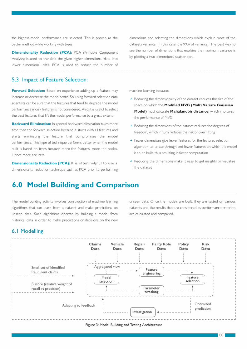
The model building activity involves construction of machine learning
algorithms that can learn from a dataset and make predictions on
unseen data. Such algorithms operate by building a model from
historical data in order to make predictions or decisions on the new
5.3 Impact of Feature Selection:
6.1 Modelling
the highest model performance are selected. This is proven as the
better method while working with trees.
Dimensionality Reduction (PCA): PCA (Principle Component
Analysis) is used to translate the given higher dimensional data into
lower dimensional data. PCA is used to reduce the number of
dimensions and selecting the dimensions which explain most of the
datasets variance. (In this case it is 99% of variance). The best way to
see the number of dimensions that explains the maximum variance is
by plotting a two-dimensional scatter plot.
machine learning because:
Reducing the dimensionality of the dataset reduces the size of the
space on which the Modi�ed MVG (Multi Variate Gaussian
Model) must calculate Mahalanobis distance, which improves
the performance of MVG
Reducing the dimensions of the dataset reduces the degrees of
freedom, which in turn reduces the risk of over �tting
Fewer dimensions give fewer features for the features selection
algorithm to iterate through and fewer features on which the model
is to be built, thus resulting in faster computation
Reducing the dimensions make it easy to get insights or visualize
the dataset
unseen data. Once the models are built, they are tested on various
datasets and the results that are considered as performance criterion
are calculated and compared.
Figure 3: Model Building and Testing Architecture
Small set of identi�edfraudulent claims
β score (relative weight of recall vs precision)
Adapting to feedback Optimized prediction
Investigation
ClaimsData
VehicleData
RepairData
Party RoleData
PolicyData
RiskData
Aggregated view
Feature selection
Feature engineering
Model selection
Parametertweaking
09
The following steps are listed to summarize the process of the
model development:
Once the dataset is obtained and cleaned, different models are
tested on it
Based on the initial model performance, different features are
engineered and re-tested
Once all the features are engineered, the model is built and run
using different β values and using different iteration procedures
(feature selection process)
In order to improve model performance, the parameters that affect
the performance are tweaked and re-tested
Separate models generated for each fraud type which self-calibrate
over time - using feedback, so that they adapt to new data and user
behavior changes.
Multiple models are built and tested on the above datasets. Some of
them are:
Logistic Regression: Logistic regression measures the relationship
between a dependent variable and one or more independent variables
by estimating probabilities using a logit function. Instead of regression in
generalized linear model (glm), a binomial prediction is performed. The
model of logistic regression, however, is based on assumptions that are
quite different from those of linear regression. [5] In particular the key
differences of these two models can be seen in the following two
features of logistic regression. The predicted values are probabilities
and are therefore restricted to [0, 1] through the logit function as the
glm predicts the probability of particular outcomes which tends to
be binary.
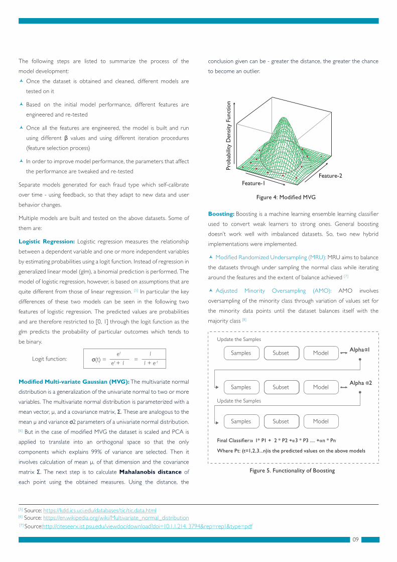
Modi�ed Multi-variate Gaussian (MVG): The multivariate normal
distribution is a generalization of the univariate normal to two or more
variables. The multivariate normal distribution is parameterized with a
mean vector, μ, and a covariance matrix, Σ. These are analogous to the
mean μ and variance σ2 parameters of a univariate normal distribution. [6] But in the case of modi�ed MVG the dataset is scaled and PCA is
applied to translate into an orthogonal space so that the only
components which explains 99% of variance are selected. Then it
involves calculation of mean μ, of that dimension and the covariance
matrix Σ. The next step is to calculate Mahalanobis distance of
each point using the obtained measures. Using the distance, the
Logit function:et
et + 1
[7] Source:http://citeseerx.ist.psu.edu/viewdoc/download?doi=10.1.1.214. 3794&rep=rep1&type=pdf
[5] Source: https://kdd.ics.uci.edu/databases/tic/tic.data.html[6] Source: https://en.wikipedia.org/wiki/Multivariate_normal_distribution
Boosting: Boosting is a machine learning ensemble learning classi�er
used to convert weak learners to strong ones. General boosting
doesn’t work well with imbalanced datasets. So, two new hybrid
implementations were implemented.
Modi�ed Randomized Undersampling (MRU): MRU aims to balance
the datasets through under sampling the normal class while iterating
around the features and the extent of balance achieved [7]
Adjusted Minority Oversampling (AMO): AMO involves
oversampling of the minority class through variation of values set for
the minority data points until the dataset balances itself with the
majority class [8]
Figure 4: Modi�ed MVG
Figure 5. Functionality of Boosting
Samples Alpha 1Subset Model
Samples Subset Model
Samples
Update the Samples
Final Classi�er: 1* P1 + 2 * P2 + 3 * P3 .... + n * Pn
Where Pt: (t=1,2,3...n)is the predicted values on the above models
Update the Samples
Subset Model
Feature-2Feature-1
Prob
abili
ty D
ensi
ty F
unct
ion
Alpha 2
conclusion given can be - greater the distance, the greater the chance
to become an outlier.
1
1 + e-tσ(t) = =

10
6.2 Model Performance Criterion
Bagging using Adjusted Random Forest: Unlike single decision
trees which are likely to suffer from high variance or high bias
(depending on how they are tuned), in this case the model classi�er is
tweaked to a great extent in order to work well with imbalanced
datasets. Unlike the normal random forest, this Adjusted or Balanced
Random Forest is capable of handling class imbalance. [9]
The Adjusted Random Forest algorithm is shown below:
In every iteration the model draws a replaceable bootstrap sample
of minority class (In this case fraudulent claims) and also draws the
same number of claims, with replacement, from the majority class
(In this case honest policy holders)
Try building a tree with the above sample (without pruning) with
the following modi�cation: The decision of split made at each node
should be based on set of mtry randomly selected features only (not
all the features)
Repeat (i) and (ii) steps n times and aggregate the �nal result and
use it as the �nal predictor
The advantage of Adjusted Random Forest is that it doesn’t over�t as
it performs tenfold cross-validations at every level of iteration. The
functionality of ARF is represented in the form of a diagram below.
6.2.1 Using Contingency Matrix or Error Matrix
The Model performance can be evaluated using different measures. Some of them used in this paper are:
[8] Source: https://www3.nd.edu/~dial/papers/ECML03.pdf[9] Source: http://statistics.berkeley.edu/sites/default/�les/tech-reports/666.pdf [10] Source: http://www2.cs.uregina.ca/~dbd/cs831/notes/confusion_matrix/confusion_matrix.html [11] Source: http://www2.cs.uregina.ca/~dbd/cs831/notes/confusion_matrix/confusion_matrix.html
Figure 6. Functionality of Bagging using Random Forests
Training set (with m records)
Draw samples (with replacement)
PF
Training set (with n records) Training set (with n records)
Voting
Final Prediction
Aggregation of votes
Training set (with n records) t - Bootstraps sets
t - Prediction sets......
......
P1 P2 Pt
True Negatives (TN)
True Positives (TP)
False Negatives (FN)
False Positives (FP)
Actual
Normal
Normal
Fraud
Fraud
Predicted
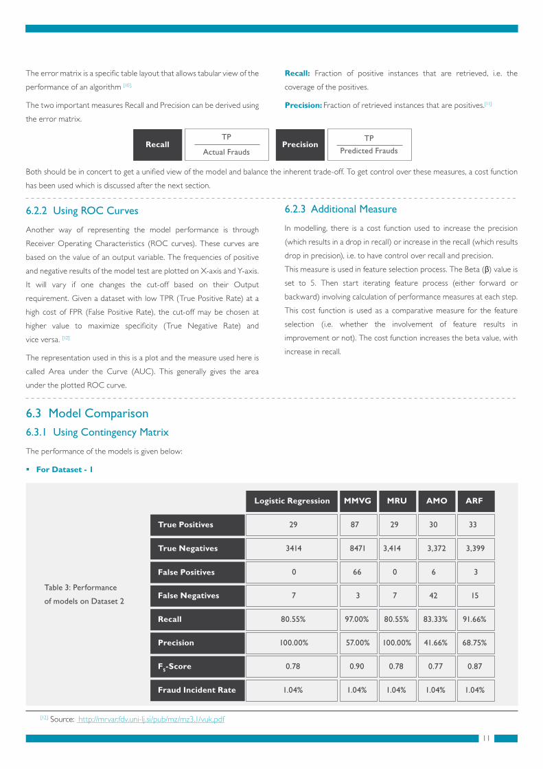
Table 3: Performance
of models on Dataset 2
11
The error matrix is a speci�c table layout that allows tabular view of the
performance of an algorithm [10].
The two important measures Recall and Precision can be derived using
the error matrix.
6.2.2 Using ROC Curves
Another way of representing the model performance is through
Receiver Operating Characteristics (ROC curves). These curves are
based on the value of an output variable. The frequencies of positive
and negative results of the model test are plotted on X-axis and Y-axis.
It will vary if one changes the cut-off based on their Output
requirement. Given a dataset with low TPR (True Positive Rate) at a
high cost of FPR (False Positive Rate), the cut-off may be chosen at
higher value to maximize speci�city (True Negative Rate) and
vice versa. [12]
The representation used in this is a plot and the measure used here is
called Area under the Curve (AUC). This generally gives the area
under the plotted ROC curve.
6.3 Model Comparison6.3.1 Using Contingency Matrix
The performance of the models is given below:
For Dataset - 1
Both should be in concert to get a uni�ed view of the model and balance the inherent trade-off. To get control over these measures, a cost function
has been used which is discussed after the next section.
Recall: Fraction of positive instances that are retrieved, i.e. the
coverage of the positives.
Precision: Fraction of retrieved instances that are positives.[11][11]
6.2.3 Additional Measure
In modelling, there is a cost function used to increase the precision
(which results in a drop in recall) or increase in the recall (which results
drop in precision), i.e. to have control over recall and precision.
This measure is used in feature selection process. The Beta (β) value is
set to 5. Then start iterating feature process (either forward or
backward) involving calculation of performance measures at each step.
This cost function is used as a comparative measure for the feature
selection (i.e. whether the involvement of feature results in
improvement or not). The cost function increases the beta value, with
increase in recall.
[12] Source: http://mrvar.fdv.uni-lj.si/pub/mz/mz3.1/vuk.pdf
Logistic Regression
True Positives
True Negatives
False Positives
False Negatives
Recall
Precision
F5-Score
Fraud Incident Rate
29
3414
0
7
80.55%
100.00%
0.78
1.04%
87
8471
66 0
3
97.00%
57.00%
0.90
1.04%
29
3,414
7
80.55%
100.00%
0.78
1.04%
30
3,372
6
42
83.33%
41.66%
0.77
1.04%
33
3,399
3
15
91.66%
68.75%
0.87
1.04%
MMVG MRU AMO ARF
RecallTP
Actual FraudsPrecision
TP
Predicted Frauds

Key note: All the models performed better on this dataset (with nearly ninety times improvement over the incident rate). Relatively, MMVG has
better recall and the other models have better precision.
Key note: The ensemble models performed better with high values of recall and precision. Comparatively ARF has high precision and high recall
(i.e. 1666 times better than the incident rate) and MMVG has better recall but poor precision.
Key note: MRU (with four hundred and sixty times improvement over random guess) and MMVG (with hundred and thirty three times improvement
over the incident rate and reasonably good recall) are better performers and logistic regression is a poor performer.
For Dataset - 2
For Dataset - 3
12
Logistic Regression
True Positives
True Negatives
False Positives
False Negatives
Recall
Precision
F5-Score
Fraud Incident Rate
77
238006
11
50
67.3%
46.87%
0.63
0.06%
347
587293
4609
26
93.00%
7.00%
0.63
0.06%
79
238029
9
27
88.46%
66.66%
0.84
0.06%
86
236325
2
1731
82.05%
27.94%
0.73
0.06%
86
236325
6
11
95.51%
80.54%
0.91
0.06%
MMVG MRU AMO ARF
Logistic Regression
True Positives
True Negatives
False Positives
False Negatives
Recall
Precision
F5-Score
Fraud Incident Rate
105
224635
51
119
87.5%
60.62%
0.82
0.03%
212
590043
5098 18
7
97.00%
4.00%
0.51
0.03%
138
224685
69
89.77%
74.52%
0.85
0.03%
128
224424
28
330
97.72%
4.73%
0.54
0.03%
149
224718
7
36
93.18%
88.17%
0.89
0.03%
MMVG MRU AMO ARF
13
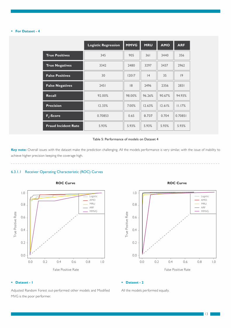
Key note: Overall issues with the dataset make the prediction challenging. All the models performance is very similar, with the issue of inability to
achieve higher precision keeping the coverage high.
Adjusted Random Forest out-performed other models and Modi�ed
MVG is the poor performer.
Table 5: Performance of models on Dataset 4
For Dataset - 4
6.3.1.1 Receiver Operating Characteristic (ROC) Curves
Dataset - 1
All the models performed equally.
Dataset - 2
Logistic Regression
True Positives
True Negatives
False Positives
False Negatives
Recall
Precision
F5-Score
Fraud Incident Rate
345
3342
30
2451
92.00%
12.33%
0.70853
5.93%
905
2480
12017 14
18
98.00%
7.00%
0.65
5.93%
361
3297
2496
96.26%
12.63%
0.737
5.93%
3440
3437
35
2356
90.67%
12.61%
0.704
5.93%
356
2962
19
2831
94.93%
11.17%
0.70851
5.93%
MMVG MRU AMO ARF
False Positive Rate
ROC Curve
True
Pos
itive
Rat
e
0.0
0.0
0.2
0.4
0.6
0.8
1.0
0.2 0.4 0.6 0.8 1.0
Logistic
MRU
AMO
ARF
MMVG
False Positive Rate
ROC Curve
True
Pos
itive
Rat
e
0.0
0.0
0.2
0.4
0.6
0.8
1.0
0.2 0.4 0.6 0.8 1.0
Logistic
MRU
AMO
ARF
MMVG
14
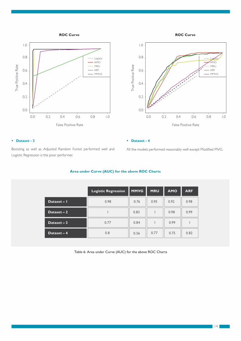
Boosting as well as Adjusted Random Forest performed well and
Logistic Regression is the poor performer.
Table 6: Area under Curve (AUC) for the above ROC Charts
Dataset - 3
All the models performed reasonably well except Modi�ed MVG.
Area under Curve (AUC) for the above ROC Charts
Dataset - 4
Logistic Regression
Dataset – 1
Dataset – 2
Dataset – 3
Dataset – 4
0.98
1
0.77
0.8
0.76
0.83
0.84
0.56
1
0.95
0.77
1
0.92
0.98
0.99
0.75
0.98
0.99
0.82
1
MMVG MRU AMO ARF
False Positive Rate
ROC Curve
True
Pos
itive
Rat
e
0.0
0.0
0.2
0.4
0.6
0.8
1.0
0.2 0.4 0.6 0.8 1.0
Logistic
MRU
AMO
ARF
MMVG
False Positive Rate
ROC Curve
True
Pos
itive
Rat
e
0.0
0.0
0.2
0.4
0.6
0.8
1.0
0.2 0.4 0.6 0.8 1.0
Logistic
MRU
AMO
ARF
MMVG

15
The analysis indicates that the modi�ed random under Sampling and
Adjusted Random Forest algorithms perform best. However, it cannot
be assumed that the order of predictive quality would be replicated for
other datasets. As observed in the dataset samples, for feature rich
datasets, most models perform well (ex: Dataset - 1). Likewise, in cases
with signi�cant quality issues and limited feature richness the model
performance gets degraded (ex: Dataset - 4).
Key Takeaways:
Predictive quality depends more on data than on algorithm:
Many researches [13][14] indicate quality and quantity of available data has
a greater impact on predictive accuracy than quality of algorithm. In the
analysis, given data quality issues most algorithms performed poorly on
dataset-4. In the better datasets, the range of performance was
relatively better.
Poor performance from logistic regression and relatively
poor performance by odi�ed MVG:
Logistic regression is more of a statistical model rather than a machine
To display the effective usage of the cost function measure, a graph of
results is shown for different β values (1, 5, and 10) and modelled on
dataset-1. As evident from the results, there is a correlation between β
Figure 8. Model Performances for Different Beta Values
120
100
80
60
40
AMO AMO AMO ARF ARF ARF LM LM LM MRU MRU MRU MVG MVG MVG1 5 10 1 5 10 1 5 10 1 5 10 1 5 10
20
0
6.3.2 Model Performances for Different Values in Cost Function Fβ
value and recall percentage. Typically this also results in static or
decrease in precision (given implied trade-off). This is manifested
across models, except for AMO at a β value of 10.
7.0 Model Verdict
In this analysis, many factors were identi�ed which allows for an
accurate distinction between fraudulent and honest claimants i.e.
predict the existence of fraud in the given claims. The machine learning
models performed at varying performance levels for the different input
datasets. By considering the average F5 score, model rankings are
obtained- i.e. a higher average F5 score is indicative of a better
performing model.
learning model. It fails to handle the dataset if it is highly skewed. This
is a challenge in predicting insurance frauds, as the datasets will typically
be highly skewed given that incidents will be low.
MMVG is built with an assumption that the input data supplied is of
Gaussian distribution which might not be the case. It also fails to handle
categorical variables which in turn are converted to binary equivalents
which leads to creation of dependent variables. Research also indicates
that there is a bias induced by categorical variables with multiple
potential values (which leads to large number of binary variables.)
Outperformance by Ensemble Classi�ers:
Both the boosting and bagging being ensemble techniques, instead of
learning on a single classi�er, several are trained and their predictions
are aggregated. Research indicates that an aggregation of weak
classi�ers can out-perform predictions from a single strong performer.
Loss of Intuition with Ensemble Techniques
A key challenge is the loss of interpretability because the �nal
combined classi�er is not a single tree (but a weighed collection of
multiple trees), and so people generally lose visual clarity of a single
classi�cation tree. However, this issue is common with other classi�ers
like SVM (support vector machines) and NN (neural networks) where
the model complexity inhibits intuition. A relatively minor issue is that
while working on large datasets, there is signi�cant computational
complexity while building the classi�er given the iterative approach
with regard to feature selection and parameter tweaking. Anyhow
given model development is not a frequent activity this issue will not be
a major concern.[15]
Table 7: Performance of Various Models
Model Name
Logistic Regression
MMVG
MRU
AMO
0.38
0.59
0.79
0.57
1
5
3
4
Avg. F5 Score Rank
ARF 0.73 2
The analysis indicates that the modi�ed random under Sampling and
Adjusted Random Forest algorithms perform best. However, it cannot
be assumed that the order of predictive quality would be replicated for
other datasets. As observed in the dataset samples, for feature rich
datasets, most models perform well (ex: Dataset - 1). Likewise, in cases
with signi�cant quality issues and limited feature richness the model
performance gets degraded (ex: Dataset - 4).
Key Takeaways:
Predictive quality depends more on data than on algorithm:
Many researches [13][14] indicate quality and quantity of available data has
a greater impact on predictive accuracy than quality of algorithm. In the
analysis, given data quality issues most algorithms performed poorly on
dataset-4. In the better datasets, the range of performance was
relatively better.
Poor performance from logistic regression and relatively
poor performance by odi�ed MVG:
Logistic regression is more of a statistical model rather than a machine
8.0 Conclusion
The machine learning models that are discussed and applied on the
datasets were able to identify most of the fraudulent cases with a low
false positive rate i.e. with a reasonable precision. This enables loss
control units to focus on new fraud scenarios and ensuring that the
models are adapting to identify them. Certain datasets had severe
challenges around data quality, resulting in relatively poor levels
of prediction.
Given inherent characteristics of various datasets, it would be
impractical to a' priori de�ne optimal algorithmic techniques or
recommended feature engineering for best performance. However, it
would be reasonable to suggest that based on the model performance
on back-testing and ability to identify new frauds, the set of models
offer a reasonable suite to apply in the area of insurance claims fraud.
The models would then be tailored for the speci�c business context
and user priorities.
9.0 Acknowledgements
The authors acknowledges the support and guidance of Prof. Srinivasa
Raghavan of International Institute of Information Technology, Bangalore.
16
[13] Source: http://people.csail.mit.edu/torralba/publications/datasets_cvpr11.pdf[14] Source: http://www.csse.monash.edu.au/~webb/Files/BrainWebb99.pdf[15] Source: http://www.stat.cmu.edu/~ryantibs/datamining/lectures/24-bag-marked.pdf
learning model. It fails to handle the dataset if it is highly skewed. This
is a challenge in predicting insurance frauds, as the datasets will typically
be highly skewed given that incidents will be low.
MMVG is built with an assumption that the input data supplied is of
Gaussian distribution which might not be the case. It also fails to handle
categorical variables which in turn are converted to binary equivalents
which leads to creation of dependent variables. Research also indicates
that there is a bias induced by categorical variables with multiple
potential values (which leads to large number of binary variables.)
Outperformance by Ensemble Classi�ers:
Both the boosting and bagging being ensemble techniques, instead of
learning on a single classi�er, several are trained and their predictions
are aggregated. Research indicates that an aggregation of weak
classi�ers can out-perform predictions from a single strong performer.
Loss of Intuition with Ensemble Techniques
A key challenge is the loss of interpretability because the �nal
combined classi�er is not a single tree (but a weighed collection of
multiple trees), and so people generally lose visual clarity of a single
classi�cation tree. However, this issue is common with other classi�ers
like SVM (support vector machines) and NN (neural networks) where
the model complexity inhibits intuition. A relatively minor issue is that
while working on large datasets, there is signi�cant computational
complexity while building the classi�er given the iterative approach
with regard to feature selection and parameter tweaking. Anyhow
given model development is not a frequent activity this issue will not be
a major concern.[15]
10.0 Other References
The Identi�cation of Insurance Fraud – an Empirical Analysis - by
Katja Muller. Working papers on Risk Management and Insurance
no: 137, June 2013.
Minority Report in Fraud Detection: Classi�cation of Skewed Data
- by Clifton Phua, Damminda Alahakoon, and Vincent Lee. Sigkdd
Explorations, Volume – 6, Issue – 1.
A Novel Anomaly Detection Scheme Based on Principal
Component Classi�er, M.-L. Shyu, S.-C. Chen, K. Sarinnapakorn, L.
Chang, A novel anomaly detection scheme based on principal
component classi�er, in: Proceedings of the IEEE Foundations and
New Directions of Data Mining Workshop, Melbourne, FL, USA,
2003, pp. 172–179.
Anomaly detection: A survey, Chandola et al, ACM Computing
Surveys (CSUR), Volume 41 Issue 3, July 2009.
Machine Learning, Tom Mitchell, McGraw Hill, 199.
Hodge, V.J. and Austin, J. (2004) A survey of outlier detection
methodologies. Arti�cial Intelligence Review.
Introduction to Machine Learning, Alpaydin Ethem, 2014, MIT Press.
Quinlan, J. (1992). C4.5: Programs for Machine Learning. Morgan
Kaufmann, San Mateo, CA.
17
Pazzani, M., Merz, C., Murphy, P., Ali, K., Hume, T., & Brunk, C.
(1994). Reducing Misclassi�cation Costs. In Proceedings of the
Eleventh International Conference on Machine Learning San
Francisco, CA. Morgan Kauffmann.
Mladeni c, D., & Grobelnik, M. (1999). Feature Selection for
Unbalanced Class Distribution and Naive Bayes. In Proceedings of
the 16th International Conference on Machine Learning. pp.
258–267. Morgan Kaufmann
Japkowicz, N. (2000). The Class Imbalance Problem: Signi�cance
and Strategies. In Proceedings of the 2000 International Conference
on Arti�cial Intelligence (IC-AI’2000): Special Track on Inductive
Learning Las Vegas, Nevada
Bradley, A. P. (1997). The Use of the Area under the ROC Curve in
the Evaluation of Machine Learning Algorithms. Pattern
Recognition, 30(6), 1145–1159.
Insurance Information Institute. Facts and Statistics on Auto
Insurance, NY, USA, 2003.
Fawcett T and Provost F. “Adaptive fraud detection”, Data
Mining and Knowledge Discovery, Kluwer, 1, pp 291-316, 1997.
Drummond C and Holte R. “C4.5, Class Imbalance, and Cost
Sensitivity: Why Under-Sampling beats Over-Sampling”, in Workshop
on Learning from Imbalanced Data Sets II, ICML, Washington DC,
USA, 2003.

18
11.1 About the Authors
He drives strategic initiatives at Wipro with focus around building productized capability in Big Data and Machine Learning. He
leads the Apollo product development and its deployment globally. He can be reached at: [email protected]
R GuhaHead - Corporate Business Development
Shreya ManjunathProduct Manager, Apollo Platforms Group
Kartheek PalepuAssociate Data Scientist, Apollo Platforms Group
She leads the product management for Apollo and liaises with customer stakeholders and across Data Scientists, Business
domain specialists and Technology to ensure smooth deployment and stable operations. She can be reached at:
He researches in Data Science space and its applications in solving multiple business challenges. His areas of interest include
emerging machine learning techniques and reading data science articles and blogs. He can be reached at:

DO BUSINESS BETTER
CONSULTING | SYSTEM INTEGRATION | BUSINESS PROCESS SERVICES
WIPRO L IMITED , DODDAKANNELL I , SAR JAPUR ROAD, BANGALORE - 560 035 , INDIA . TEL : +91 (80) 2844 0011 , FAX : +91(80) 2844 0256 , Ema i l : in fo@wipro . com
Wipro Ltd. (NYSE:WIT) is a leading Information Technology, Consulting and Business Process Services company that delivers solutions to enable its clients do business better. Wipro delivers winning business outcomes through its deep industry experience and a 360 degree view of "Business through Technology" - helping clients create successful and adaptive businesses. A company recognized globally for its comprehensive portfolio of services, a practitioner's approach to delivering innovation, and an organization-wide commitment to sustainability,Wipro has a workforce of over 150,000, serving clients in 175+ cities across 6 continents.
For more information, please visit www.wipro.com
About Wipro Ltd.
North America Canada Brazil Mexico Argentina United Kingdom Germany France Switzerland Nordic Region Poland Austria Benelux Portugal Romania Africa Middle East India China Japan Philippines Singapore Malaysia South Korea Australia New Zealand
WIPRO LIMITED 2015© IND/BRD/NOV 2015-JAN 2017