common trends and shocks to top incomes: a structural breaks approach

1

Common Trends and Shocks to Top Incomes:

A Structural Breaks Approach

Jesper Roine�† and Daniel Waldenström

March 06, 2010

Abstract

We use newly compiled top income share data and structural breaks techniques to es-timate common trends and breaks in inequality across countries over the twentieth century. Our results both confirm earlier findings and offer new insights. In particular, the division into an Anglo-Saxon and a Continental European experience is not as clear cut as previously suggested. Some Continental European countries seem to have experienced increases in top income shares, just as Anglo-Saxon countries, but typi-cally with a lag. Most notably, Nordic countries display a marked �“Anglo-Saxon�” pat-tern, with sharply increased top income shares especially when including realized capital gains. Our results help inform theories about the causes of the recent rise in inequality.

Keywords: Top incomes, income inequality, economic development, common struc-tural breaks JEL: C320, D310, N300

We have received valuable comments from Andrew Leigh, Henry Ohlsson, Thomas Piketty, two

anonymous referees and seminar participants at Centre Emile Bernheim, Université Libre de Bruxelles and at the 3rd BETA Workshop, Université Louis Pasteur Strasbourg. We are also grateful to Jushan Bai, Pierre Perron and Zhongjun Qu for making their GAUSS programs available. �† SITE, Stockholm School of Economics, P.O. Box 6501, SE-11383 Stockholm, Ph: +46-8-7369682, E-mail: [email protected] IFN, P.O. Box 55665, SE-10215 Stockholm, Ph: +46-8-6654531, E-mail: [email protected].

2

1 Introduction

Over the past years a collective research project dedicated to creating detailed and

comparable series of long-run top income shares has resulted in a number of new in-

sights about income inequality.1 These series, covering a number of mostly developed

countries, have highlighted the importance of decomposing the top of the distribution,

both into smaller fractions and with respect to the source of income, so as to better

understand what has driven changes in income inequality.2

A key aspect of the new series is the improvement they constitute in terms compara-

bility. Several studies have suggested that the new homogenous data now makes

cross-country comparisons of long-run trends more meaningful and that such com-

parisons can give important keys to constructing theories about developments of ine-

quality. A broad conclusion from these studies has been that inequality in most devel-

oped countries has trended downward in a surprisingly homogenous fashion during

the first three quarters of the twentieth century, but also that the most recent decades

display important divergences. In particular, it has been emphasized that while top

income shares have increased dramatically in Anglo-Saxon countries, the develop-

ment in Continental Europe has been much more stable since around 1980.3 This in

turn has cast some doubts on theories where, for example, technological change, or

other developments that have been common across Western countries, are the main

drivers of changes in inequality.4

1 Atkinson and Piketty (2007, 2009) collect and comments on much of this work. See also Piketty (2005), Piketty and Saez (2006) and Leigh (2009) for overviews of the top income literature. 2 Key insights include that much of the decline in inequality in the first half of the Twentieth Century was in fact driven by sharp drops (rather than gradual decreases) in the income share of a small top group (top one percent or smaller). The main cause seems to have been shocks to capital incomes (rather than changes in wage shares) associated with events such as the World Wars and the Great De-pression. For the more recent past the detailed study of shares within the top decile again shows that much of the increases in inequality have been driven by the top percent, but this time mostly based on gradually rising income shares for top wage earners (rather than capital). Besides highlighting the im-portance of decomposing the top and studying different sources of income this has also shown the im-portance of annual data. Connecting single observations too far apart can not distinguish between theo-ries of gradual change and those where shocks are the main cause of change 3 The title of the first collected volume of top income research, Top Incomes over the Twentieth Cen-tury: A Contrast between European and English-Speaking Countries (Atkinson and Piketty, 2007), illustrates the importance of contrasting English speaking countries and Continental Europe. 4 For example, Piketty and Saez (2006) argue that theories claiming that technological progress have made managerial skills more general and less firm specific, thus creating a �“super-star�” environment for the best executives, can not explain the observed patterns in the data. It could potentially explain the

3

These conclusions have so far been based on casual observation of the time-series. In

some cases, as with the shocks of the Great Depression or World War II, the breaks in

data are very sharp and easily identifiable. The same goes for the relatively homoge-

nous long-run trend of decreasing inequality across countries over the first three quar-

ters and the great variability in terms of the reversal of this trend after the 1970s.

However, when it comes to specifying exactly when the upward trend of increased

inequality begins in various countries, or when it comes to identifying if countries can

be said to experience a common development, and if so, what this common develop-

ment looks like, it is much more difficult to determine these things just by eyeballing

the data.

The aim of this paper is to provide rigorous answers to questions regarding structural

breaks and common trends in inequality over the long run. We want to use available

data to find the statistical answer to questions such as: Are there structural breaks, i.e.,

statistically robust shifts in means and trends, in inequality over time? If so, when do

these breaks occur? To what extent are they common for countries or groups of coun-

tries?

Our approach is to use recent econometric techniques, both for estimating breaks for

individual countries one at the time (Bai and Perron, 1998, 2003) as well as estimating

breaks jointly for groups of countries (Qu and Perron, 2007). This allows us to iden-

tify breaks which are common for all countries, breaks which are common for groups

of countries, as well as breaks which seem unique for individual countries. Studying

the trends in the periods between the estimated breaks also allows us to see which

countries have had similar developments over different periods and to group countries

according to such trends.

Studying if there are common breaks and trends in the series, as well as finding poten-

tial similarities or differences between countries, is important for formulating possible

increases in Anglo-Saxon countries but not the fact that top income shares have not gone up in Europe and Japan where the technological developments have been similar.

4

theories to explain developments of inequality.5 We do not claim that our technical

approach is better than conclusions reached by looking at the time-series, but we do

believe that our approach is an important complement to previous casual observations.

Many of our results largely confirm what has been suggested in previous work, but we

also find a number of interesting new results. With respect to what drives the move-

ments of the top decile we confirm the previous finding that most of the drops across

countries come from the top of the distribution, while the lower half of the top decile

experiences relatively little long-run movement (trends between the identified breaks

are essentially flat). With respect to common breaks in the first half of the century our

results are also in line with the previous literature indicating that the Second World

War does indeed constitute a structural break in the top income shares in countries

directly involved in the war. However, countries that did not directly participate, such

as Sweden and Switzerland, have no structural breaks at this point in time. We also

find that the World War II break constitutes a divide between a prior period of sharply

declining top percentile income shares and a subsequent period of continued, but less

pronounced, decreasing inequality.

However, the common continued declining trend, according to our structural breaks

analysis, ends around 1980 and is followed by increases almost everywhere. (Ger-

many, the Netherlands, and Switzerland are the only exceptions where breaks are not

followed by an increase but of a leveling out of the previous decrease). We find in-

creases in inequality trends in Continental Europe but in particular in the Nordic coun-

tries. In terms of timing our results suggest that the increases start in the US and the

UK which are then followed by Australia, Ireland and New Zealand together with

Sweden, Finland and Norway where increases are at least as pronounced as in some

Anglo-Saxon countries (however, starting from lower levels). Portugal and Spain also

seem to have increasing top income shares (though data is only available for the top

0.1 percent group) and given the recent increases in France the trend there is also ris-

5 For example, in a different context Perron (1989) illustrates the importance of identifying breaks in a number of macroeconomic variables for the question of whether these variables have a unit root (against the alternative that they are trend-stationary).

5

ing.6 These findings have clear implications for the alternative explanations for recent

increases in inequality.

2 Econometric methodology

The empirical analysis rests on new developments in the literature on estimating

structural breaks in univariate and multivariate time series. We define �“structural

breaks�” as statistically significant and lasting shifts in the mean or the trend (or both).

Throughout the breaks are treated as unknown, which essentially means that they are

estimated endogenously from the time series properties without imposing prior no-

tions about their existence or timing. Previous research has found this approach to be

superior to estimating beforehand known breaks (Perron, 2005).

This study uses two methods to detect and estimate structural breaks in top income

shares. The Qu and Perron (2007) method estimates multiple common breaks for sev-

eral countries and the Bai and Perron (1998, 2003) method estimates multiple breaks

in individual country time series. Both of these methods are well-known in the time

series econometrics literature.7 The Bai and Perron method has been widely used and

Monte Carlo simulations have shown it to be robust to both persistent and trending

regressors as well as serial correlation, heteroskedasticity and differently distributed

residuals across regimes (Bai and Perron, 2006). The Qu and Perron method relies on

largely the same asymptotic theory. It is more recent and has not yet been applied to

the same extent. In fact, our study is one of the first empirical applications of it.8

We start by specifying linear models of top income shares. When estimating common

structural breaks in top income shares across countries using the Qu and Perron

(2007) method, we regress a vector of log of top percentile income shares on the vec-

tors of constants, linear time trends and random errors as follows:

6 It is important to note that some of our �“new�” conclusions are results of using data for more countries, and for slightly longer time periods, rather than results of the structural breaks analysis. 7 There are, however, several other techniques available. For example, in the case of estimating one or more unknown breaks in univariate time series Zivot and Andrews (1992), Banerjee, Lumsdaine and Stock (1992) and Andrews (1993). There are fewer tests for common breaks, but among the ones pre-sented are Bai, Lumsdaine and Stock (1998), Bai (1997) and Hansen (2003). 8 We have only found two other (still unpublished) studies that also use the Qu and Perron method: Bataa et al. (2008) and Chouliarakis (2008), who both use it for estimating breaks and trends in infla-tion.

6

t t j ty I z S u , t = Tj�–1 ,..., Tj �– 1. (1)

In equation (1), yt = (y1t, ..., ynt) denotes an n-country vector of logged top income

shares, I the identity matrix, zt = (z1t, ..., zqt) a vector with q regressors where zit =

{1,t}t for country i (i = 1, ..., n) and year t. S is a selection matrix, j a vector of coeffi-

cients estimated separately for each of the j regimes (j = 1, 2, ..., m�–1, where m is the

maximum number of breaks) and ut is a random error.9 The equivalent model for es-

timating breaks in univariate series, using the Bai and Perron (1998, 2003) method,

looks as follows:

t j j ty c t , t = Tj�–1 ,..., Tj �– 1, (2)

where, again, yt is a country-specific top income share in log, cj intercept and tj time

trend, both estimated separately for segments j, and t is a random error term.

A central parameter to be defined in all the estimations is the trimming value, which is

the share of the series corresponding to the shortest time that a break needs to last in

order to qualify as �“structural�”. There is a trade-off associated with deciding the

trimming parameter. If one requires periods to be too long that potentially leads to

missing �“true shifts�” in the series. Conversely, a too short minimum break length

could lead to short-lived �“noise�” being captured as a structural break in the series. In

this paper, we use a rule of thumb saying that breaks should last at least one business

cycle, which we implement as being at least eight years. Since our analyzed top in-

come share series differ in length this means that we will actually use different trim-

ming parameters in the estimations.10

9 We use top income shares in logarithms since this allows us to interpret trends as average annual per-centage change in the top income shares. Our results are robust to using logs or not. In the analysis of common breaks, only two minor discrepancies were found when not using logs (the all-country post-war break was found in 1985 instead of 1983, and the second break in the Anglo-Saxon century series was found in 1958 instead of 1953). 10 We are in some cases also restricted by the model specifications. This is particularly true when ap-plying the Qu and Perron methodology, since we estimate both means and trends for multiple series and for this need a fairly large number of observations. In practice, we therefore use trimming values corresponding to minimum segment lengths well beyond one business cycle.

7

When testing for existence, number, and timing of the breaks, we follow a setup that

is common for both Bai and Perron and Qu and Perron methodologies.11 In short, the

tests use a recursive approach in which the linear equations are estimated for different

sets of intercepts and linear trends corresponding to different combinations of break

points. At each possible combination, a Likelihood Ratio-test (Qu and Perron method)

or F-test (Bai and Perron method) is conducted in order to examine whether a statisti-

cally significant break occurred or not. If it did, the procedures continue to determine

the exact number of breaks and their location using recursive selection methods.12 Fi-

nally, after having estimated the exact number and timing of the breaks have been de-

fined the resulting model is fitted and intercept and trend coefficients estimated.13

There are a few practical concerns with the application of, in particular, the Qu and

Perron methodology. For example, it requires the analyzed panels to be balanced, i.e.,

that they begin and end at the same point in time. Given the quite large variation in

start and end years in our top income dataset (see further the data section), this implies

that we are confined to using relatively short panels, beginning in the latest starting

year and ending in the earliest ending year. One effect of this requirement is that we

can only include countries with sufficiently long time series.14

In the case of the Bai and Perron method, we mainly use the so-called �“sequential

method�” (which adds one break each time the test is significant) to determine the

number of breaks. Throughout, however, we corroborate this approach by referring to

the number of breaks found by other commonly employed information criteria, esti-

mated in the GAUSS programs constructed by method creators, and use these criteria

if the F-statistic of the final models estimated is larger than in the model suggested by

the sequential method. In several cases, the exact sets of breaks estimated differ

11 For details see Qu and Perron (2007), Bai and Perron (1998, 2003) and Perron (2005). 13 An important point regarding the interpretation of the exact timing of the breaks is that they should not necessarily be thought of as something �“happening�” in the particular year when the break is identi-fied. In some cases, there is really an abrupt shock that creates a lasting shift in a trend, but more com-monly the shift happens gradually and in these cases the exact timing should be given less weight when interpreting the results. Here the break is simply the statistical answer to the question: When can we say that a lasting shift in trend happened given a certain trimming value (determining what we consider �“structural�”)? 14 For example, our tests of common breaks over the whole century exclude Germany (earliest observa-tion for which we can create continuous annual series is 1947), Singapore (1947), Switzerland (1933), the United Kingdom (1949). See further the discussion in the data section.

8

somewhat across models. Typically the sequential method detects more breaks than

the information criteria and when it differs its model typically produces a lower F-

statistic. This selection among models is a problematic aspect of the multivariate

breaks methodology and it adds a certain degree of discretion. Our ambition has there-

fore been to implement the selection approach consequently and it appears to have

little impact in itself on the overall results of the study.15

3 Data

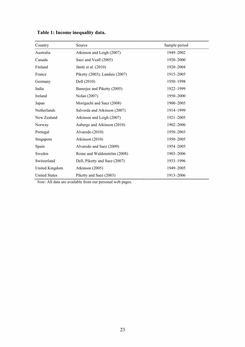
The data come from newly generated series of top income shares covering a total of

18 countries over most of the twentieth century (see Table 1).16 The main source for

the income data is personal income tax returns on the national level. Income shares

are calculated following a methodology first outlined in Piketty (2001, 2003).17 The

basic idea is to construct shares of total personal income received by different fractiles

of the entire (tax) population, had everyone been required to file a tax return. Since

the reference total for population includes individuals who have not filed a tax return,

and the reference total for income includes their incomes as well as other incomes that

do not appear in tax records, these totals must be constructed using aggregate sources

from the population statistics and national accounts. Top income shares are then com-

puted by dividing the number of tax units in the top, and their incomes, with the refer-

ence tax population and reference total income. The income reported is typically gross

total income and includes income from labor, business and capital (but in most cases

not realized capital gains) before taxes and transfers.18

[Table 1 here] 15 There are a few cases of variation across selection procedures in terms of both number and timing of estimated breaks. However, we deem that this variation does not concern large and significant breaks but rather to what extent minor, and mostly economically insignificant breaks, are statistically signifi-cant or not. 16 Coverage varies both in terms time periods and in terms of fractiles for which we have data. For Ire-land, Portugal and Spain we only have long-run series for the top 0.1 percentile share and not the top percentile which we use for other countries. The income shares of the top 1 and top 0.1 percentile groups are, however, generally highly correlated (>0.9) and hence almost interchangeable in a time series analysis such as this. For some countries data do not extend before World War II. This means, for example, that we have different samples when estimating common breaks over all of the twentieth century, as compared to the period 1950 and onward. Throughout we try our best to be explicit with exactly why we do what we do as well as with checking alternative specifications. 17 Piketty (2001, 2003) in turn builds on the seminal work by Kuznets (1953). 18 Occasionally, the authors compiling data for individual countries were unable to separate out realized capital gains from other sources of capital income. In particular, this has been the case for Norway and to some extent Australia and New Zealand.

9

Despite the explicit efforts to make the series consistent and comparable some known

discrepancies remain in the data. Some differences in both income and income earner

(tax unit) definitions remain. For example, realized capital gains are excluded from

the income concept in all countries except for Australia, New Zealand and (partly) the

UK. Tax unit definitions vary even more. In Australia, Canada, China, India and

Spain they are individuals but in Finland, France, Ireland, the Netherlands, Switzer-

land and the United States they are households (i.e., married couples or single indi-

viduals). Moreover, in Japan, New Zealand, Sweden and the United Kingdom the tax

authorities switched from household to individual filing. In Germany there is a mix-

ture of the two, with the majority of taxpayers being household tax units whereas the

very rich filing as individuals. When comparing the estimated trend breaks with the

major dates of changes in data definitions for single countries or country groups, we

cannot find any important temporary correlations except for a few cases.19

Another source of measurement variation is that the tax year is not the same as the

calendar year in some countries, e.g., Australia, New Zealand, and U.K. Following

Atkinson and Piketty (2007), we use tax years throughout moved to the nearest calen-

dar year (e.g., the U.K. tax year between April 1986 and March 1987 becomes 1986

in our data). When comparing our results with structural breaks estimates for Austra-

lia and New Zealand using smoothed series (averaging parts of tax years to fit calen-

dar years), we find no discrepancies. For a longer and more detailed discussion of

these problems, see Atkinson and Piketty (2007, chapter 13) and Leigh (2009).

Missing values, often due to a lack of information in the national tax statistics, are

linearly interpolated in order to make the series continuous and possible to analyze

with the econometric techniques outlined in Section 2. Of course, interpolating series

is not ideal and implies that we merge observations drawn from completely different

data generating processes. The problems related to interpolation are the biggest in the

case of Norway and Sweden before 1930, when we have only a handful of years of

observations since 1902. In these cases, the interpolations are so long that we can not

19 There are two cases in which we cannot rule out the impact of administrative changes on the esti-mated break: Netherlands in 1977 (when the underlying income data source changed) and Sweden in 1991 (when a large tax reform changed the definitions of income on tax returns).

10

be confident that the series reflect all the actual time series variation. On the other

hand we are concerned with lasting structural breaks and at least for shorter interpo-

lated periods it seems unlikely that the interpolations would affect the estimated

breaks. Also, for the postwar period, which is our main period of analysis, there are

few gaps and the existing ones are too short for the interpolation to interfere with our

results.

4 Results

As discussed above the methodology to detect common breaks offers a way of finding

statistically robust structural changes (i.e., lasting shifts in the mean and/or the trend)

that are not always obvious from merely inspecting the series. We begin by studying

such structural changes across all countries to find episodes which are important

enough to cause �“global�” shifts over the whole of the twentieth century.20 Then we

look at common breaks for certain groups of countries (Anglo-Saxon, Continental

Europe, Scandinavia and Asia) for the same, full time span. After that we focus on the

postwar period 1950�–2006 and rerun the common break analyses and also analyze

each country individually to see if there are important variations from the aggregate

picture(s). The reason for limiting the more detailed analysis to the latter period is

twofold. First, this period is the longest that fulfills criteria of having sufficiently de-

tailed, homogenous data for analyzing structural breaks for the individual countries.

Second, much of the debate over postwar inequality shifts have focused on the most

recent couple of decades and by shortening the window of analysis we gain precision

in the structural breaks estimation.

4.1 Common breaks over the whole of the twentieth century

Looking first at breaks common for the top percentile income share across all coun-

tries over the whole of the twentieth century, displayed in Table 2, we find that the

end of World War II (1945) constitutes a shift from a sharper decline (in the period

before that year) to a continued but slower decline. The postwar equalization ends in

the beginning of the 1980s (1981) when top income shares either start increasing or

remain at historically low levels.

20 Clearly, �“global�” here refers to our data set and naturally the estimation is limited to the subset of countries for which we have data over the whole period.

11

[Figure 1 here]

[Table 2 here]

As previously has been pointed out in the top income literature, it is informative to

contrast the development of the share of the top percentile group with that of the low-

est half of the top income decile (P90�–95). In most countries this group consists of

high wage earners, with only marginal contributions from capital and performance

pay schemes. The income share for this group has been remarkably stable over the

twentieth century. Although the procedure detects two common structural breaks in

the postwar period, these are relatively minor.

[Figure 2 here]

A second step in the analysis is to divide the sample into subgroups of countries and

study their common breaks and trends. We have chosen to extend the division in the

previous top income literature where two country groups are emphasized: Anglo-

Saxon countries (Australia, Canada, New Zealand, United Kingdom and the United

States) and Continental European countries (France, Germany, Netherlands, Switzer-

land). Beside these we also form a group of Nordic countries (Finland, Norway and

Sweden) and a group of Asian countries (India, Japan and Singapore).21 As the panels

in Figure 3 show the break points for the country groups remain relatively close to the

ones found to be common for all countries suggesting these breaks are indeed global

rather than driven by specific country or country group characteristics. Again, when it

comes to the impact of World War II this is hardly surprising, but when it comes to

21 One obvious alternative grouping suited for a specific but important question is to distinguish be-tween countries that directly took part in World War II and those that did not. Analyzing these groups shows what is already obvious to the naked eye namely that the war was devastating to top income earners, but mainly in countries that took active part in the war. Naturally, all countries were affected by wartime trade disruptions and regulations, but the bombings of factories and other capital destroying events (including extraordinary regulatory or taxation interventions) were probably graver to the in-comes of the rich in belligerent countries. Another possibility is to include Japan in the group of Conti-nental European countries. This would make sense if one aims at studying different �“welfare state re-gimes�”, using the terminology of Esping-Andersen (1990), where Japan best fits the corporatist tradi-tion which in turn corresponds roughly to the Continental European countries. This would, however, only be reasonable for a more recent sub-period than for the whole of the twentieth century. The chosen grouping of Scandinavian countries we think makes sense in terms of these having many things in common while the particular Asian group is, as we will discuss later, much less homogenous. In fact, apart from geography it is hard to find a priori reasons for why they should constitute a group.

12

the latter break around 1980 it is less obvious what is driving the shift (we will come

back to this when we analyze the period 1950�–2006 in more detail below).22

[Figure 3 here]

Overall, our analysis of the first half of the century does not provide any startling new

insights, but rather underlines what has been pointed out before. The decline in top

income shares was driven mostly by drops in the top percentile, and this, in turn, was

mainly driven by shocks incurred during, in particular, World War II.

4.2 Structural breaks in the period 1950�–2006

We now turn to analyzing common patterns across countries during the postwar pe-

riod. This period offers a more homogenous dataset, with annual observations avail-

able throughout for practically all countries in our sample. In Figure 4 we present the

estimate on the �“global�” sample. The Qu and Perron method detects one common

break during this period, estimated in 1983. The average growth rates in top income

shares before and after this break listed in Table 2 suggest that this break marks a shift

between two eras: one era of steady decline in inequality followed by a new era of

increasing top income shares.23

[Figure 4 here]

When splitting the full sample into the four country groups introduced above, some

quite notable dissimilarities in postwar inequality trends are revealed.24 Figure 5

shows how Nordic, Continental and Asian countries experienced periods of equaliza-

tion or accelerated equalization trends in the 1960s whereas no such pattern is found

for Anglo-Saxon countries. Around the mid-1970s, the postwar compression halted in 22 A somewhat surprising point regarding the impact of World War II, as noted in Atkinson and Piketty (2007), is that WW II did not have a sharp negative effect on top incomes in Australia and New Zea-land and also that top incomes in both these countries increased markedly just after the war. 23 Note that we in Table 2 report the yearly percentage change between two break years, including the shift in intercept. This means that a level change that happens at the break point is smoothed out over following period. We use the fitted trends (based on unweighted country averages for the common breaks) when calculating these yearly changes. 24 It is worth emphasizing that we, in this section, are treating the countries as a group. In some cases it is relatively clear that one country does not behave as the rest of the group but one of the points of this particular exercise is precisely to find common breaks and trends when forcing some countries to form a group. Individual country breaks will be analyzed in the next section.

13

both Continental and Anglo-Saxon countries but not in Nordic and Asian countries

where it continued a little longer. After the 1970s, top income shares remained on

their historically low levels in Continental countries. In the group of Anglo-Saxon

countries, however, we estimate a significant trend break in 1987 after which the top

percentile went from stable levels to growing by 2.8 percent per year. Interestingly the

Nordic countries also experienced a reversal of the postwar compression, but not until

1991.25 It is worth noting that the estimated yearly percentage increase for the Nordic

group is even higher than the increase in the Anglo-Saxon countries, but, of course,

starting from a much lower level.26

[Figure 5 here]

Up until this point we have only studied the incidence of common structural trend

breaks in various groupings of countries. Even though such analysis is warranted for

reasons already discussed, it is still important to supplement it with country case stud-

ies as there are of course important differences between individual countries. We start

by looking more closely at the individual Anglo-Saxon countries, shown in Figure 6

and Table 3. The figures show that the upward trend in top income shares starts in the

late 1970s in the US, Canada and in the UK. Only about five to ten years later do we

see the same kind of upturn in Australia, New Zealand and Ireland (though Ireland has

a short term peak around 1980).

[Figure 6 here]

[Table 3 here]

Looking at the other country group exhibiting sharp inequality increases in recent

decades, the Nordic countries in Figure 7, we note that the trend breaks seem to have

occurred in two stages in all three countries. First, the postwar compression stopped in

the early 1980s and about a decade later inequality started to grow rapidly. The reason

for why the common break procedure previously only detected the second break date

25 On the exact timing of this break, however; see the caveat mentioned in Section 3, footnote 18 above. 26 Taking the common break trends literally the Nordic countries are today at the same level of inequal-ity (top percentile share of about eight percent) as the Anglo-Saxon countries had at the break in 1986.

14

is purely technical (only one break could be estimated within this relatively short time

period and the 1990s break apparently dominated the 1980s break).

[Figure 7 here]

Turning to the individual countries of Continental Europe in Figure 8, we note a pat-

tern that is rather diverse. As seen above the average development has been one of

very modest increases in top income shares but countries such as Spain and Portugal

exhibit clear increases over the past decades (in the case of Spain this has been going

on since the 1960s). France also seems to be on a path of increasing inequality, at

least since the mid 1990s. Germany does not seem to exhibit any clear trend over the

past decades, while Switzerland and the Netherlands have slightly downward trending

top income shares. While it is certainly true that the development in Continental

Europe is not characterized by the same sharp increases that we see in the Anglo-

Saxon countries and more recently in Scandinavia, the development is not really one

common development of unchanged top income shares either.

[Figure 8 here]

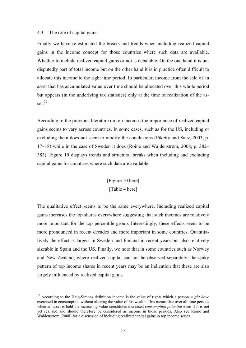
Finally, looking at the breaks and trends in Japan, India and Singapore shows three

very different experiences. In Japan, where top income shares fell sharply during

World War II, the development has been relatively stable since 1950 (somewhat simi-

lar to the development in Germany). India on the other hand exhibits the more �“stan-

dard�” pattern with top income shares falling significantly until around 1980 when they

started to increase at about the same pace as they had been falling up until then. In

Singapore, finally, the top share decreased sharply in the 1950s and 1960s and re-

mained low up to the Asian crisis in 1997 when it increased rapidly. Studying these

individual country experiences suggests that a grouping of these particular countries

into an Asian group does not seem to make much sense.

[Figure 9 here]

15

4.3 The role of capital gains

Finally we have re-estimated the breaks and trends when including realized capital

gains in the income concept for those countries where such data are available.

Whether to include realized capital gains or not is debatable. On the one hand it is un-

disputedly part of total income but on the other hand it is in practice often difficult to

allocate this income to the right time period. In particular, income from the sale of an

asset that has accumulated value over time should be allocated over this whole period

but appears (in the underlying tax statistics) only at the time of realization of the as-

set.27

According to the previous literature on top incomes the importance of realized capital

gains seems to vary across countries. In some cases, such as for the US, including or

excluding them does not seem to modify the conclusions (Piketty and Saez, 2003, p.

17�–18) while in the case of Sweden it does (Roine and Waldenström, 2008, p. 382�–

383). Figure 10 displays trends and structural breaks when including and excluding

capital gains for countries where such data are available.

[Figure 10 here]

[Table 4 here]

The qualitative effect seems to be the same everywhere. Including realized capital

gains increases the top shares everywhere suggesting that such incomes are relatively

more important for the top percentile group. Interestingly, these effects seem to be

more pronounced in recent decades and more important in some countries. Quantita-

tively the effect is largest in Sweden and Finland in recent years but also relatively

sizeable in Spain and the US. Finally, we note that in some countries such as Norway

and New Zealand, where realized capital can not be observed separately, the spiky

pattern of top income shares in recent years may be an indication that these are also

largely influenced by realized capital gains.

27 According to the Haig-Simons definition income is the value of rights which a person might have exercised in consumption without altering the value of his wealth. This means that over all time periods when an asset is held the increasing value constitutes increased consumption potential even if it is not yet realized and should therefore be considered as income in those periods. Also see Roine and Waldenström (2008) for a discussion of including realized capital gains in top income series.

16

5 Concluding discussion

Even though documenting the common breaks and trends can be interesting in its own

right the underlying question is of course: What can we learn from the results above?

In what way does this analysis contribute to a better understanding of what has driven

inequality over the long run? We believe that we offer three main additions to what

has previously been suggested in terms of finding commonalities in the developments

of inequality based on top income shares. First, our results indicate that the Nordic

countries actually may have more in common with the Anglo-Saxon group than with

Continental Europe in terms of changes in top income shares. The sharp increase

comes somewhat later but in terms of trend the percentage increases have, in fact,

been higher in the Nordic countries in recent decades.28 The overall levels are lower

than in the US, the UK and Canada, but even in level terms the Nordic countries seem

to be almost as �“Anglo-Saxon�” as Australia and New Zealand. Second, we find that

including realized capital gains may be more important than what has previously been

suggested, especially in the Nordic countries. Third, and finally, our results also indi-

cate that Continental Europe may be more heterogeneous than previously suggested.

In particular, Spain and Portugal, and to some extent France, display increasing top

income shares in recent years, while only Germany, the Netherlands and Switzerland

have flat or decreasing trends after 1980.29

Our results cast some doubt on attempts to attribute differences in inequality across

countries�—in terms of pre-tax, market outcomes�—to differences in their �“social-

political-economic systems�” (see, e.g., Mishel, Bernstein and Allegretto, 2007). When

dividing countries into being more or less �“egalitarian�” the Nordic countries are typi-

cally seen as most egalitarian while the Anglo-Saxon countries are at the other ex-

treme with Continental Europe in between. This pattern, however, is not reflected in

the recent top income developments. A possible explanation is that aspects such as the

degree of centralized wage bargaining, the importance of unions, whether society is

28 As already mentioned in Section 2 above, even though the breaks are clearly not to be interpreted as something happening at the exact year identified by the method, we think they are far enough apart for it to be relevant to say that the trend reversal comes first in the US and the UK, later in other Anglo-Saxon countries, and yet later in the Scandinavian countries. 29 This point is not in conflict with the previous emphasis on the contrast between Anglo-Saxon and Continental European countries in Atkinson and Piketty (2007) and other previous papers but rather a consequence of us being able to include more countries for slightly longer time periods than what was available before.

17

characterized by a �“consensus model�” or is more �“competitive�”, etc. are all likely to

be important for overall wage inequality (and for redistribution) but are unlikely to be

the main factors behind what has happened recently to pre-tax income in the top per-

centile group in the Nordic countries.30

When thinking about alternative explanations to the observed patterns with respect to

the similarities between Nordic and Anglo-Saxon countries, a number of features

come to mind. First, stock market values in the Nordic countries have soared since the

early 1980s when compared to most other countries in the sample (see Roine and

Waldenström, 2008). If executive compensation increases in proportion to stock mar-

ket value, as suggested by Gabaix and Landier (2008), this could certainly explain the

disproportionate increases in top income shares in Scandinavia.31 It would also make

sense that part of this would show as realized capital gains, especially given the dual

tax system in these countries where tax levels are lower for capital gains than for

wage income.32 Relating to this point, Roine, Vlachos and Waldenström (2009) find

that financial development (measured as stock market capitalization to income) is

strongly pro rich in a cross section of countries. Other features common to the Nordic

countries that may play a role are that they are all small open economies with an im-

portant share of large multinational firms, and also that English (though a second lan-

guage) is commonly spoken in the population.33 If it is the case that these to a larger

extent compete for �“superstars�” on a global rather than a national level this could help

explain the disproportionate increase in the top, in line with Rosen (1981).34

30 See also Scheve and Stasavage (2009) for empirical evidence questioning the importance of labor market institutions as drivers of long-run income inequality. 31 On the other hand, this can not be the full explanation since stock market increases in, e.g., France have been of the same magnitude as in the US and the UK with very different resulting inequality pat-terns. 32 Obviously the tax legislation is typically constructed so that there should not be such tax arbitrage possibilities. However, in practice it seems likely that this happens anyway. 33 Saez and Veall (2005) find that wages of anglophones (more likely to migrate to the US and hence with a better bargaining position) have increased more than those of the French speakers. Even though it is by no means clear that a stronger position of English as a second language in Scandinavia in gen-eral, implies that executives in these countries be more likely to compete on the international market compared to executives in Continental European countries, where English is less common as a spoken language, it is a possible channel that would be interesting to explore further. 34 On a more speculative note it is possible that exposure to US executive education has been higher in Scandinavia than in Continental Europe and that this would have created a more Anglo-Saxon �“pay culture�” in these countries through channels similar to those in Spilimbergo (2009).

18

Finally, our results that the Continental European development may be more hetero-

geneous than previously suggested means that there may be reasons for looking closer

at differences across Continental European countries. Given that the split seems to be

between on the one hand Spain, Portugal, and to some extent France, and, on the other

hand, Germany, the Netherlands, and Switzerland, one could of course start to specu-

late about some kind of Latin-Germanic divide. At this stage, however, collecting data

for more European countries, to see if such a divide is there when including more

countries, seems more important.

19

References

Aaberge, Rolf and Anthony B. Atkinson, �“Top Incomes in Norway�”, in Anthony B. Atkinson and Thomas Piketty (Eds.), Top Incomes: A Global Perspective. Vol-ume II, (Oxford: Oxford University Press, 2010).

Alvaredo, Facundo, �“Top Incomes and Earnings in Portugal 1936�–2005�”, in Anthony B. Atkinson and Thomas Piketty (Eds.), Top Incomes: A Global Perspective. Volume II, (Oxford: Oxford University Press, 2010).

Alvaredo, Facundo and Emmanuel Saez, �“Income and Wealth Concentration in Spain from a Historical and Fiscal Perspective,�” Journal of the European Economic Association 7:5 (2009), 1140�–1167.

Andrews Donald W. K., �“Tests for Parameter Instability and Structural Change with Unknown change Point,�” Econometrica 61:4 (1993), 821�–856.

Atkinson, Anthony B., �“Top Incomes in the United Kingdom over the Twentieth Cen-tury,�” Journal of the Royal Statistical Society 168:2 (2005), 325�–343.

Atkinson, Anthony B., �“Top Incomes in a Rapidly Growing Economy: Singapore�”, in Anthony B. Atkinson and Thomas Piketty (Eds.), Top Incomes: A Global Per-spective. Volume II, (Oxford: Oxford University Press, 2010).

Atkinson, Anthony B. and Andrew Leigh, �“The Distribution of Top Incomes in New Zealand�” (pp. 333�–365), in Anthony B. Atkinson and Thomas Piketty (Eds.), Top Incomes over the Twentieth Century: A Contrast between European and English-Speaking Countries, (Oxford: Oxford University Press, 2007).

Atkinson, Anthony B. and Andrew Leigh, �“The Distribution of Top Incomes in Aus-tralia�” (pp. 309�–332), in Anthony B. Atkinson and Thomas Piketty (Eds.), Top Incomes over the Twentieth Century: A Contrast between European and Eng-lish-Speaking Countries, (Oxford: Oxford University Press, 2007).

Atkinson, Anthony B. and Thomas Piketty (Eds.), Top Incomes over the Twentieth Century: A Contrast between European and English-Speaking Countries, (Ox-ford: Oxford University Press, 2007).

Bai, Jushan, �“Estimation of a Change Point in Multiple Regression Models,�” this RE-VIEW 79:4 (1997), 551�–563.

Bai, Jushan, Robin L. Lumsdaine and James H. Stock, �“Testing For and Dating Common Breaks in Multivariate Time Series,�” Review of Economic Studies 65:3 (1998), 395�–432.

Bai, Jushan and Pierre Perron, �“Estimating and Testing Linear Models with Multiple Structural Changes,�” Econometrica 66:1 (1998), 47�–78.

Bai, Jushan and Pierre Perron, �“Computation and Analysis of Multiple Structural Change Models,�” Journal of Applied Econometrics 18:1 (2003), 1�–22.

20

Bai, Jushan and Pierre Perron, �“Multiple Structural Change Models: A Simulation Analysis�”, in Dean Corbea, Stephen Durlauf and Bruce E. Hansen (Eds.), Econometric Theory and Practice: Frontiers of Analysis and Applied Research, (Cambridge, Cambridge University Press, 2006).

Banerjee, A., Lumsdaine, R. L. and Stock, J. H., �“Recursive and sequential tests of the unit root and trend-break hypothesis,�” Journal of Business and Economic Statis-tics 10:3 (1992), 271�–288.

Bataa, E. D. R. Osborn, M. Sensier, D. van Dijk, �“Identifying Changes in Mean, Sea-sonality, Persistence and Volatility for G7 and Euro Area Inflation�”, unpub-lished manuscript (2008).

Chouliarakis, George, P. K. G. Harischandra, �“Do Exchange Rate Regimes Matter for Inflation Persistence? Theory and Evidence from the History of UK and US In-flation�”, unpublished manuscript (2008).

Dell, Fabien, �“Top Incomes in Germany throughout the Twentieth Century�” (pp. 365�–425), in Atkinson, Anthony B. and Thomas Piketty (Eds.), Top Incomes over the Twentieth Century: A Contrast between European and English-Speaking Coun-tries, (Oxford: Oxford University Press, 2007).

Dell, Fabien, Thomas Piketty and Emmanuel Saez, �“Income and Wealth Concentra-tion in Switzerland of the 20th Century�” (pp. 472�–500), in Anthony B. Atkinson and Thomas Piketty (Eds.), Top Incomes over the Twentieth Century: A Con-trast between European and English-Speaking Countries, (Oxford: Oxford Uni-versity Press, 2007).

Dew-Becker, Ian and Robert J. Gordon, �“Where Did the Productivity Growth Go? Inflation Dynamics and the Distribution of Income,�” Brooking Papers on Eco-nomic Activity 2 (2005), 67�–127.

Esping-Andersen, G., The Three Worlds of Welfare Capitalism, (Cambridge, UK: Pol-ity Press, Blackwell Publishers, 1990).

Hansen, Bruce E., �“The New Econometrics of Structural Change: Dating Breaks in U.S. Labor Productivity�”, Journal of Economic Perspectives 15:4 (2001), 117�–128.

Jäntti, Markus, Marja, Riihelä, Risto Sullström and Matti Tuomala, �“Trends in Top Income Shares in Finland�”, in Anthony B. Atkinson and Thomas Piketty (Eds.), Top Incomes: A Global Perspective. Volume II, (Oxford: Oxford University Press, 2010).

Gabaix, Xavier and Augustin Landier, �“Why has CEO Pay Increased so Much?,�” Quarterly Journal of Economics 123:1 (2008), 49�–100.

Gersbach, Hans and Armin Schmutzler, �“Does Globalization Create Superstars?�”, CEPR discussion paper no. 6222 (2008).

Gordon, Robert J. and Ian Dew-Becker, �“Controversies about the Rise of American Inequality: A Survey�”, NBER Working Paper no. 13982, (2008).

21

Kuznets, Simon, Shares of Upper Income Groups in Income and Savings, New York: National Bureau of Economic Research, 1953).

Landais, Camille, �“Les hauts revenus en France (1998�–2006), Une explosion des inégalités ?�”, unpublished manuscript (2007).

Leigh, Andrew, �“Top Incomes�” (pp. 150�–174), in Wiemer Salverda, Brian Nolan and Timothy Smeeding (Eds.), The Oxford Handbook of Economic Inequality, (Ox-ford, Oxford University Press, 2009).

Manasse, Paolo and Alessandro Turrini, �“Trade, Wages, and �‘Superstars�’,�” Journal of International Economics 54:1 (2001), 97�–117.

Mishel, Lawrence, Jared Bernstein and Sylvia Allegretto, The State of Working Amer-ica 2006/2007, (Ithaca, NY: ILR Press, 2007).

Mookherjee, Dilip, and Debraj Ray, �“Occupational Diversity and Endogenous Ine-quality,�” unpublished manuscript (2006).

Moriguchi, Chiaki and Emmanuel Saez, �“The Evolution of Income Concentration in Japan, 1885�–2002: Evidence from Income Tax Statistics,�” this REVIEW 90:4 (2008), 713�–734.

Nolan, Brian, �“Long-Term Trends in Top Income Shares in Ireland�” (pp. 501�–530), in Anthony B. Atkinson and Thomas Piketty (Eds.), Top Incomes over the Twenti-eth Century: A Contrast between European and English-Speaking Countries, (Oxford: Oxford University Press, 2007).

O�’Rourke, Kevin H., �“Globalization and Inequality: Historical Trends,�” Annual World Bank Conference on Development Economics 2 (2001), 39�–67.

O�’Rourke, Kevin H. and Jeffrey G. Williamson, �“After Columbus: Explaining the Global Trade Boom 1500�–1800,�” Journal of Economic History 62:2 (2002), 417�–456.

Perron, Pierre, �“The Great Crash, the Oil Price Shock and the Unit Root Hypothesis,�” Econometrica 57:6 (1989), 1361�–1401.

Piketty, Thomas, Les hauts revenus en France au 20ème siècle, (Grasset, Paris, 2001).

Piketty, Thomas, �“Income Inequality in France, 1900�–1998,�” Journal of Political Economy 111:5 (2003), 1004�–1042.

Piketty, Thomas, �“Top Income Shares in the Long Run: An Overview,�” Journal of the European Economic Association 3:2�–3 (2005), 1�–11.

Piketty, Thomas and Emmanuel Saez, �“Income Inequality in the United States, 1913�–1998,�” Quarterly Journal of Economics 118:1 (2003), 1�–39.

Piketty, Thomas and Emmanuel Saez, �“The Evolution of Top Incomes: A Historical and International Perspective,�” American Economic Review, Papers and Pro-ceedings 96:2 (2006), 200�–205.

22

Qu, Zhongjun and Perron, Pierre, �“Estimating and Testing Multiple Structural Changes in Multivariate Regressions,�” Econometrica 75:2 (2007), 459�–502.

Roine, Jesper, Vlachos, Jonas and Daniel Waldenström, �“The Long-Run Determinants of Inequality: What Can We Learn from Top Income Data?,�” Journal of Public Economics 93:7�–8 (2009), 974�–988.

Roine, Jesper and Daniel Waldenström, �“The Evolution of Top Incomes in an Egali-tarian Society: Sweden, 1903�–2004,�” Journal of Public Economics 92:1�–2 (2008), 366�–387.

Saez, Emmanuel and Michael R. Veall, �“The Evolution of High Incomes in Northern America: Lessons from Canadian Evidence,�” American Economic Review 95:3 (2005), 831�–849.

Salverda, Wiemer and Anthony B. Atkinson, �“Top Incomes in the Netherlands over the Twentieth Century�” (pp. 426�–471), in Anthony B. Atkinson and Thomas Piketty (Eds.), Top Incomes over the Twentieth Century: A Contrast between European and English-Speaking Countries, (Oxford: Oxford University Press, 2007).

Scheve, Ken and David Stasavage, �“Institutions, Partisanship, and Inequality in the Long Run,�” World Politics 61:2 (2009), 215�–253.

Spilimbergo, Antonio, �“Democracy and Foreign Education,�” American Economic Re-view 99:1 (2009), 528�–43.

Zivot, Eric and Andrews, Donald W. K., �“Further evidence on the great crash, the oil price shock and the unit root hypothesis,�” Journal of Business and Economic Statistics 10:3 (1992), 251�–270.

23

Table 1: Income inequality data.

Country Source Sample period

Australia Atkinson and Leigh (2007) 1949�–2002

Canada Saez and Veall (2005) 1920�–2000

Finland Jäntti et al. (2010) 1920�–2004

France Piketty (2003); Landais (2007) 1915�–2005

Germany Dell (2010) 1950�–1998

India Banerjee and Piketty (2005) 1922�–1999 Ireland Nolan (2007) 1950�–2000

Japan Moriguchi and Saez (2008) 1900�–2005

Netherlands Salverda and Atkinson (2007) 1914�–1999

New Zealand Atkinson and Leigh (2007) 1921�–2005

Norway Aaberge and Atkinson (2010) 1902�–2006

Portugal Alvaredo (2010) 1950�–2003

Singapore Atkinson (2010) 1950�–2005

Spain Alvaredo and Saez (2009) 1954�–2005

Sweden Roine and Waldenström (2008) 1903�–2006

Switzerland Dell, Piketty and Saez (2007) 1933�–1996

United Kingdom Atkinson (2005) 1949�–2005

United States Piketty and Saez (2003) 1913�–2006 Note: All data are available from our personal web pages.

24

Table 2: Common cross-country trend breaks in the top 1% income share.

Yearly change in top percentile income share (%) Country group

Estimated structural breaks [95% confidence interval]

t1 t2 t3 t4 1. Global

a. Century 1945 1980 �–1.3 �–1.2 +1.8 [-44,-46] [-79,-81] b. Postwar period 1983 �–1.3 +2.2

[-81,-82] 2. Anglo�–Saxon

a. Century 1937 1953 1982 �–0.7 �–2.3 �–1.2 +2.6 [-36,-38] [-52,-54] [-81,-83] b. Postwar period 1974 1987 �–1.5 +0.1 +2.6

[-73,-75] [-85,-87] 3. Continental Europe

a. Century 1943 1976 �–1.9 �–1.2 �–0.9 [-41,-44] [-74,-77] b. Postwar period 1968 1981 +0.0 �–2.0 �–0.1

[-67,-69] [-80,- 82] 4. Nordic

a. Century 1939 1961 1991 �–0.5 �–1.4 �–2.4 +4.2 [-38,-42] [-60,-62] [-90,-92] b. Postwar period 1965 1981 1992 �–0.1 �–2.7 �–0.3 +3.9

[-64,-66] [-80,-82] [-91,-93] 5. Asia

a. Century 1945 1959 1983 �–1.2 +0.5 �–0.2 +0.8 [-44,-46] [-58,-60] [-82,-84] b. Postwar period 1961 1974 1984 �–0.8 �–1.6 �–1.1 +1.7 [-60,-62] [-73,-76] [-83,-85]

Note: The table presents statistically significant breaks in logged top percentile income shares esti-mated using the method of Qu and Perron (2007). For country sample selection, see the text. Yearly changes in top shares during segments, tj (j = 1,2.3,4), are the compounded percentage change between start and ending years calculated from fitted break trends on country group averages. Country samples and time periods: 1a: Australia, Canada, Finland, France, Japan, New Zealand, Norway, Sweden, United States, 1921�–2000. 1b: Australia, Canada, Finland, France, India, Japan, Netherlands, New Zealand, Norway, Singapore, Sweden, United Kingdom, United States, 1950�–2000. 2a: Australia, Canada, New Zealand, United States, 1921�–2000. 2b: Australia, Canada, United Kingdom, New Zealand, United States, 1950�–2000. 3a: France, Netherlands, 1915�–1999. 3b: France, Germany, Netherlands, Switzerland, 1950�–1999. 4a: Finland, Norway, Sweden, 1921�–2004. 4b: Finland, Norway, Sweden, 1950�–2004. 5a: India, Japan, 1922�–1999. 5b: India, Japan, Singapore, 1950�–1999.

25

Table 3: Country-specific trend breaks in top 1% income shares after 1950.

Yearly change in top percentile income share (%) Country Estimated structural breaks

[95% confidence interval] t1 t2 t3 t4 t5

Australia 1985 �–2.5 +2.5 [-84,-86] Canada 1977 1994 �–0.8 +1.6 +6.1 [-75,-78] [-93,-95] Finland 1971 1984 1997 +0.6 �–8.8 +2.0 +3.0 [-70,-72] [-83,-85] [-96,-98] France 1960 1982 1990 1998 +0.4 �–1.2 +2.4 �–1.4 +0.8 [-59,-61] [-81,-83] [-89,-91] [-97,-99] Germany 1960 1987 �–0.2 �–1.0 �–0.4 [-59,-61] [-86,-89] India 1971 1983 �–1.7 �–5.5 +1.6 [-70,-72] [-82,-84] Ireland (Top 0.1) 1979 1986 �–4.3 �–6.3 +5.3 [-76,-80] [-86,-91] Japan 1974 +0.4 +0.7 [-71,-75] Netherlands 1969 1976 �–1.6 �–6.3 �–0.6 [-68,-70] [-75,-77] New Zealand 1989 �–1.4 +1.4 [-88,-90] Norway 1993 �–1.6 +4.3 [-91,-94] Portugal (Top 0.1) 1971 1981 1990 �–0.9 �–14.3 +12.4 +3.4 [-70,-72] [-80,-82] [-89,-91] Singapore 1970 1998 �–1.5 �–0.1 +2.0 [-69,-73] [-96,-99] Spain (Top 0.1) 1961 1974 1986 1998 �–6.3 +4.3 +1.3 �–0.5 +2.7 [-61,-62] [-73,-74] [-83,-87] [-97,-01] Sweden 1968 1981 1991 �–0.7 �–3.9 +1.3 +1.3 [-67,-69] [-80,-82] [-90,-92] Switzerland 1973 +0.6 �–0.3 [-72,-74] United Kingdom 1960 1978 1996 �–3.1 �–2.4 +4.1 +1.2 [-59,-61] [-77,-79] [-93,-97] United States 1963 1978 1988 1997 �–2.2 �–0.3 +2.9 +0.9 +1.5 [-61,-64] [-77,-79] [-87,-89] [-96,-98]

Note: Structural breaks estimations using the method of Bai and Perron (1998, 2003). The dependent variable is log of top percentile income shares. Estimated trend coefficients are calculated from the fitted break trends. For Ireland, Portugal and Spain we use the top 0.1% share instead of the top 1% share for reasons of data availability as explained in the text. Yearly changes in top shares during seg-ments, tj (j = 1,2,3,4,5), are the compounded percentage change between start and ending years calcu-lated from fitted break trends.

26

Table 4: Capital gains effect: trend breaks in top 1% income shares after 1950.

Average yearly change in top per-centile income share (%) Country Estimated structural breaks

[95% confidence interval] t1 t2 t3 t4

Canada 1983 1990 �–0.7 +5.5 +4.2 [-83,-84] [-89,-92] Finland 1971 1984 1997 +0.6 �–8.8 +2.0 +3.0 [-70,-72] [-83,-85] [-95,-98] Germany 1960 1974 +0.1 �–1.5 +0.3 [-58,-61] [-73,-75] Spain (top 0.1%) 1962 1986 1994 �–6.7 +3.3 �–4.6 [-61,-63] [-85,-87] [-93,-95] Sweden 1968 1981 �–0.7 �–0.7 +2.9 [-67,-69] [-80,-81] United States 1979 �–0.8 +2.8 [-78,-80]

Note: See table 3.

27

Figure 1: Top 1% income shares, all countries, with break trend, 1900–2006.

0

5

10

15

20

25

30

1900 1920 1940 1960 1980 2000

Shareoftotalincome(%

)

Australia Canada France IndiaJapan Netherlands Norway New ZealandSweden Switzerland United Kingdom United StatesFinland Break trend

1945

1980

Note: The structural breaks shown are estimated on a 10-country group (see Table 2 for details).

28

Figure 2: Top 10%–5%, all countries, break trend included, 1900–2006.

4

6

8

10

12

14

16

1920 1940 1960 1980 2000


)

Australia Canada New Zealand United StatesFrance Netherlands Sweden NorwaySwitzerland Break trend

19751953

29

Figure 3: Country groups with break trend included, Top 1%, 1900–2006.

(a) Anglo-Saxon (b) Continental Europe

2

4

6

8

10

12

14

16

18

20

22

1910 1920 1930 1940 1950 1960 1970 1980 1990 2000


)

Australia Canada New ZealandUnited Kingdom United States Break trend

1937

1953

1981

0

5

10

15

20

25

30

1900 1920 1940 1960 1980 2000


)

France Netherlands Break trend

1943

1976

(c) Nordic (d) Asia

0

5

10

15

20

25

30

1900 1920 1940 1960 1980 2000


)

Norway Sweden Finland Break trend

1939

1961

1991

2

4

6

8

10

12

14

16

18

20

22

1900 1920 1940 1960 1980 2000


)

India Japan Break trend

1945

1964

1983

Note: The structural breaks marked in the figures are based on the estimation results in Table 2.

30

Figure 4: All countries’ top 1%, break trend included, 1950–2006.

2

4

6

8

10

12

14

16

18

1950 1960 1970 1980 1990 2000


)

Australia Canada France IndiaJapan Netherlands Norway New ZealandSweden Switzerland United Kingdom United StatesFinland Singapore Germany Break trend

1983

Note: The structural breaks shown are estimated on a 10-country group (see Table 2 for details).

31

Figure 5: Country groups’ top 1% with break trend included, 1950–2006.

(a) Anglo-Saxon (b) Continental Europe

2

4

6

8

10

12

14

16

18

1950 1960 1970 1980 1990 2000


)

Australia Canada New ZealandUnited Kingdom United States Break trend

1973

1986

2

4

6

8

10

12

14

16

18

1950 1960 1970 1980 1990 2000


)

France Netherlands SwitzerlandGermany Break trend

1967

1980

(c) Nordic (d) Asia

2

4

6

8

10

12

14

16

18

1950 1960 1970 1980 1990 2000


)

Norway Sweden Finland Break trend

1965

1981199

2

4

6

8

10

12

14

16

18

1950 1960 1970 1980 1990 2000


)

India Japan Singapore Break trend

1961

1974 1984


32

Figure 6: Anglo-Saxon countries’ top 1% with break trend included, 1950–2006.

Australia Canada

2

4

6

8

10

12

14

16

1950 1960 1970 1980 1990 2000

Share

oftotalincome(%

)

Australia Australia (break trend)

1985

6

7

8

9

10

11

12

13

14

1950 1960 1970 1980 1990 2000

Share

oftotalincome(%

)

Canada Canada (break trend)

1977

1994

Ireland (Top 0.1%) New Zealand

0.0

0.5

1.0

1.5

2.0

2.5

3.0

3.5

4.0

4.5

1950 1960 1970 1980 1990 2000


)

Ireland Ireland (break trend)

1979

1986

4

5

6

7

8

9

10

11

12

13

14

1950 1960 1970 1980 1990 2000


)

New Zealand New Zealand (break trend)

1989

United Kingdom United States

4

6

8

10

12

14

1950 1960 1970 1980 1990 2000

Share

oftotalincome(%

)

United Kingdom United Kingdom (break trend)

1960

1978

1996

6

8

10

12

14

16

18

20

1950 1960 1970 1980 1990 2000

Share

oftotalincome(%

)

United States United States (break trend)

1963 1978

1988

1997


33

Figure 7: Nordic countries’ top 1% with break trend included, 1950–2006.

Finland Norway

2

3

4

5

6

7

8

9

10

11

1950 1960 1970 1980 1990 2000

Share

oftotalincome(%

)

Finland Finland (break trend)

1971

1984

1997

2

4

6

8

10

12

14

16

18

1950 1960 1970 1980 1990 2000

Share

oftotalincome(%

)

Norway Norway (break trend)

1993

Sweden

3

4

5

6

7

8

9

1950 1960 1970 1980 1990 2000


)

Sweden Sweden (break trend)

1968

1981

1991


34

Figure 8: Continental European countries’ top 1% with break trend included, 1950–2006.

France Germany

6

7

8

9

10

11

1950 1960 1970 1980 1990 2000

Share

oftotalincome(%

)

France France (break trend)

1969

1978 19981988

8

10

12

14

1950 1960 1970 1980 1990

Share

oftotalincome(%

)

Germany Germany (break trend)

1960

1987

Netherlands Spain (Top 0.1%)

4

6

8

10

12

14

1950 1960 1970 1980 1990


)

Netherlands Netherlands (break trend)

1969

1976

0.5

1.0

1.5

2.0

2.5

3.0

1954 1964 1974 1984 1994 2004


)

Spain Spain (break trend)

1961

1974

19861997

Portugal (Top 0.1%) Switzerland

0.0

0.5

1.0

1.5

2.0

2.5

3.0

3.5

4.0

1950 1960 1970 1980 1990 2000

Share

oftotalincome(%

)

Portugal Portugal (break trend)

1971

1981

1990

7

8

9

10

11

12

1950 1960 1970 1980 1990

Share

oftotalincome(%

)

Switzerland Switzerland (break trend)

1973


35

Figure 9: Asian countries’ top 1% with break trend included, 1950–2006

Japan India

6

7

8

9

10

1950 1960 1970 1980 1990 2000

Share

oftotalincome(%

)

Japan Japan (break trend)

1974

2

4

6

8

10

12

14

16

1950 1960 1970 1980 1990

Share

oftotalincome(%

)

India India (break trend)

1971

1983

Singapore

9

10

11

12

13

14

15

16

1950 1960 1970 1980 1990 2000


)

Singapore Singapore (break trend)

1970

1998


36

Figure 10: The role of capital gains to six countries’ trend breaks, 1950–2006.

Canada Finland

6

7

8

9

10

11

12

13

14

15

16

1950 1960 1970 1980 1990 2000


)

Canada Canada (break trend)Canada Cap. gains Canada Cap. gains (break trend)

1983

1990

2

3

4

5

6

7

8

9

10

11

1950 1960 1970 1980 1990 2000


)

Finland Finland (break trend)Finland Cap. gains Finland Cap. gains (break trend)

1971

1984

1997

Germany Spain

8

9

10

11

12

13

14

1950 1960 1970 1980 1990


)

Germany Germany (break trend)Germany Cap. gains Germany Cap. gains (break trend)

1963

1974

0.5

1.0

1.5

2.0

2.5

3.0

3.5

4.0

1954 1964 1974 1984 1994 2004


)

Spain Spain (break trend)Spain Cap. gains Spain Cap. gains

1961

1986

1994

Sweden United States

3

4

5

6

7

8

9

10

11

12

1950 1960 1970 1980 1990 2000


)

Sweden Sweden (break trend)Sweden Cap. gains Sweden Cap. gains (break trend)

1968

1981

6

8

10

12

14

16

18

20

22

24

1950 1960 1970 1980 1990 2000


)

United States United States (break trend)United States Cap. gains United States Cap. gains (break trend)

1979


common trends and shocks to top incomes: a structural breaks approach

Economy & Finance

income inequality

income shares

anglosaxon countries

source of income

western countries

nordic countries

developed countries

continental european