combined strategic and operational planning - an milp success
TRANSCRIPT
Noname manuscript No.(will be inserted by the editor)
Combined Strategic and Operational Planning- An MILP Success Story in ChemicalIndustry
Josef Kallrath12
1 BASF-AG, GVC/S (Scientific Computing) - C13, D-67056 Ludwigshafen, Ger-many (e-mail: [email protected])
2 University of Florida, Astronomy Dept., Gainesville, 32661 FL, USA (e-mail:[email protected])
The date of receipt and acceptance will be inserted by the editor
Abstract We describe and solve a real world problem in chemical industrywhich combines operational planning with strategic aspects. In our simul-taneous strategic & operational planning (SSDOP) approach we develop amodel based on mixed-integer linear (MILP) optimization and apply it to areal-world problem; the approach seems to be applicable in many other sit-uations provided that people in production planning, process development,strategic and financial planning departments cooperate.
The problem is related to the supply chain management of a multi-site production network in which production units are subject to purchase,opening or shut-down decisions leading to an MILP model based on a time-indexed formulation. Besides the framework of the SSDOP approach andconsistent net present value calculations, this model includes two additionalspecial and original features: a detailed nonlinear price structure for the rawmaterial purchase model, and a detailed discussion of transport times withrespect to the time discretization scheme involving a probability concept.In a maximizing net profit scenario the client reports cost saving of severalmillions US$.
The strategic feature present in the model is analyzed in a consistentframework based on the operational planning model, and vice versa. Thedemand driven operational planning part links consistently to and influ-ences the strategic. Since the results (strategic desicions or designs) haveconsequences for many years, and depend on demand forecast, raw mate-rial availability, and expected costs or sales prices, resp., a careful sensitivityanalysis is necessary showing how stable the decisions might be with respectto these input data.
2 Josef Kallrath
Key words MILP modelling – Strategic and operational planning – Sup-ply chain – Chemical industry – Transportation
1 Introduction
This contribution evolved from a project in chemical industry in which wedeveloped and successfully applied a mixed-integer model to a real worldproblem which combines strategic and operational planning aspects in onemodel (a second example which encourages this approach is described in[9, Section 8.2]); operational planning aspects involve decisions on short ormid-term time-scale which are transformed into operational activities, e.g.,producing, shipping or selling something. Let us first give some motivationwhy this simultaneous strategic & operational planning (SSDOP) approachbased on mixed-integer optimization may greatly improve a company’s sit-uation and let us focus on some problems we might expect.
1.1 Solving design and operational planning problems simultaneously
It is a frequent experience that clients ask for support on a productionplanning or scheduling problem for a plant or reactor which just went intooperation. Often, especially in scheduling problems, it turns out that thereexist certain bottlenecks. It would greatly improve the situation if the designof a plant or reactor would be analyzed simultaneously with the planning orscheduling problem. Certainly, this problem is mathematically demandingbecause scheduling problems alone are already very difficult to solve [10],e.g., because of resources (raw material, machine availability, or personnel)too strongly limited. Thus, if the design and planning/scheduling problemare part of one embracing model this bottleneck situation might be avoided.This simultaneous approach requires the availability of realistic and detaileddemand forecast, and expected cost or sales prices, resp., and that the de-partments being responsible for the design and the planning/schedulingcooperate. The latter problem is by far the more difficult one, especially inlarge companies. A concrete example of this type, a process design networkproblem, is discussed in [9, Section 9.2].
1.2 Solving strategic and operational planning problems simultaneously
A company running a complex production network consisting of severalplants, (see, for instance, [11, Section 10.4]) wishes to buy additional plants,open new reactors based on improved technology, or to shut down someolder reactors. In their multi-stage production system there might exist log-ical implications between the status of certain reactors. The data governingthe investment or deinvestment decisions are the costs to buy a plant, or

Combined Strategic and Operational Planning 3
the costs to open or shut down a reactor. The investments or deinvest-ments should be sound over a time horizon of, say, up to 15 years. The bestapproach to analyze such situations is to develop a quantitative planningmodel and to enhance it by additional plants or reactors (leading to so-calleddesign variables and constraints) and let the model provide suggestions onoptimal design decisions. Regarding the database, it is necessary to providethe full data set (recipes, production rates and capacity, etc.) for all designplants or design reactors. All cost data should be discounted over the timehorizon in order to support a net present value analysis. Such a case for areal production division of a chemical company is discussed in Section 2.To model this problem we partly use the model formulation published in[7], [11, Section 10.4], or [13]; the current project required major extensionsrelated to design reactors, transport arriving over several time slices, non-linear pricing structures to purchase raw materials and additional objectivefunctions such as maximize net profit, multi-criteria objectives (i.e., maxi-mize profit & minimize the quantity of transport in tons), maximize salesvolume or maximize turnover.
Another problem of this type ([8] and [9, Section 9.1]), linking strategicand operational aspects is the optimization of a network of processing unitsat a large production site connected by a system of pipes. The purpose ofthis model was to design an integrated production network minimizing thecosts for raw material, investment and variable costs for re-processing units,and a cost penalty term for low product quality. The investment decisionsare considered on a 10-year linear depreciation rate.
1.3 Mathematical problems of combined models: complexity
Although company wide supply chain production models exist, see, for in-stance, [1] in most cases, because of their high complexity, even pure pro-duction planning or supply chain optimization problems are often seen asacademic and not suitable for practical application. Instead, either simplifi-cations (like linear relaxations) or simulation approaches are used, especiallyif there are several plants, tank storages, and the production planning prob-lem is just a part of the comprehensive problem of optimizing the wholesupply chain with regard to a detailed description of the commercial en-vironment, such as demands with different prices for different customers,availability of raw material or quality commitments.
Therefore, if one suggests a simultaneous strategic/design & operationalplanning (SSDOP) approach it is not a surprise that the sceptics mightargue embedding a complex mixed-integer programming model in an evenbigger problem including design features ”is by far too difficult”. Indeed, theproblem might be large and complex, but as the case discussed in Section2 shows, it is worthwhile to try and it can be done.
4 Josef Kallrath
1.4 Mathematical problems of combined models: structure of the objectivefunction
It is important that the problem is – within the limits and the assump-tions of the model – approached as an exact optimization problem with awell-defined objective function representing the economic structure of thebusiness process. We need to be able either to prove optimality, or to derivesafe bounds enabling us to compare different scenarios reliably and to per-form sensitivity analyses. A simulation approach is no substitute becauseit does not strictly (in the mathematical sense) support these items as itcould happen that the scenarios A and B have the optimal solutions 110 and105 but a simulation based approach produces best evaluations 103 and 104which would indicate that B is better. In the SSDOP approach there are afew complicating factors related to the structure of the objective function.
Since the objective function may contain terms related to operationalplanning (variable costs for production and processing, transport, raw mate-rial, utilities, inventories, mode-changes, etc.) and the design decision (eventcosts to close or open reactors, to purchase plants, etc.) the scaling in theobjective function terms might be poor. This problem might be overcomeby appropriate branching strategies and prioritizing the branching variables.Since the planning horizon considered may cover up to 15 years, nonlinear(usually concave) terms describing a price structure might enter in addition.If these terms are not too complicated they can be described sufficiently ac-curate as shown in Section 4.2, for instance.
1.5 Mathematical problems of combined models: reliability of data
A point of practical concern is the availability of demand forecast data,costs or sales prices over a long period. People not favoring the SSDOPapproach might use this as a strong argument against it. There are twoarguments to meet these concerns: a) on what grounds would they basetheir investment decisions otherwise? (the problem related to accurate dataconcerns both mathematical planning and non-mathematical planning) andb) the mathematical planning approach supports sensitivity analyses andallows to estimate the stability of the decisions with respect to variabilityof the forecast data. In addition, when building the model and collectingthe data, it is necessary to try to balance the degree of details entering themodel. Finally, depending on the specific purpose, the overall model mightbe adapted to its use on different application levels (pure strategic, pureoperational planning with fixed design decisions, etc.) requiring differentaccurateness of the data.
2 Strategic decisions in a worldwide production-network
The core production planning problem covers large parts of the supply chainincluding several plants, multi-stage production using multi-purpose reac-
Combined Strategic and Operational Planning 5
tors with some logical rules in the production scheme, tank storages, trans-port with a detailed representation of the commercial environment, suchas demands with different prices for different customers and availability ofraw material. Products are subject to aggregate demand requirements atcertain demand points. Variable costs for production, inventory, transportare given. The raw material purchase follows a nonlinear price structure.The client asked to consider the production planning problem as a partof larger problem. This larger problem comprises a production network inwhich gaseous raw materials along a line of up to six intermediate productsare converted into finished products, and in which a production unit from agiven set of design units is subject to shutdown or opening, or in which evensome whole plants can be purchased. To avoid duplication of material mostdetails of production and other features are specified in Subsection 4.1. Themost important objective is to maximize the total net profit (contributionmargin minus fixed costs minus investment costs) of the entire productionnetwork. In addition the following objective functions are maximized: con-tribution margin, total sales neglecting cost, turnover and total production.Costs can be minimized and multi-criteria objectives, for instance, maximizeprofit & minimize transport, are supported. The most relevant decision vari-ables indicate how much time per time-slice a reactor spends in a certainmode, how much of a product is produced, stored or shipped to anotherlocation. Binary variables trace the status and mode changes of a reactor.Structurally, most of the constraints are balance equations tracing invento-ries, connecting production and production recipes over several productionlevels and tracing mode changes. Other constraints relate production quan-tities, production rates and available time to each other, or guarantee thatcapacity limits are observed.
3 The mathematical model: preliminaries
3.1 The structure of the model and its basic objects
The problem sketched above has some common features with modelingmulti-purpose plants which are frequently used in the food or chemical pro-cess industry. In each mode such a reactor can produce several productsaccording to free or fixed recipes (joint production, coproduction) leadingto a general mode-product relation described by a set of yield coefficients:in a certain mode several products are produced (with different maximumdaily production rates), and vice-versa, a product can be produced in differ-ent (but not all) modes. Mode changes correspond physically, for instance,to a change of the temperature or pressure of a reactor, put the reactor ina new feasible mode and result in a considerable loss of production time,which in our case is sequence-dependent, and are modeled as a proportionallotsizing and scheduling problem (PLSP, [5, p.150]), i.e., based on time-indexed formulations with at most one setup- or mode-change per period;see also [12] for a survey on lot sizing problems.

6 Josef Kallrath
We thus transform the problem into a model describing a multi-site pro-duction network including multi-stage production in plants (a plant hostingsets of reactors) depending on the mode chosen for the reactors. Parts ofthe model have already been published in [7], [11, Section 10.4], or [13]; thecurrent project required major extensions related to design reactors, trans-port arriving over several time slices, nonlinear pricing structures to pur-chase raw materials and additional objective functions such as maximize netprofit, multi-criteria objectives (i.e., maximize profit & minimize the quan-tity of transport in tons), maximize sales volume or maximize turnover. Wethus extend and develop an elaborated version of the model [11, Section10.4]. In our model we use the following set of objects and indices:
b ∈ B := {1, . . . , NB} : break points (nonlinear price function)c ∈ C := {1, . . . , NC} : sales categoriesd ∈ D := {1, . . . , ND} : demand pointsk ∈ Ks := {1, . . . , NK
s } : production periods at site sm ∈Msr := {1, . . . , NM
sr } : modes at site s for reactor rp ∈ P := {1, . . . , NP } : productsr ∈ R := {1, . . . , NR} : reactorss ∈ S := {1, . . . , NS} : production sites / plantst ∈ T := {1, . . . , NT } : commercial periods
Break points are points at which the unit price as a function of volumechanges. Sales categories allow, for instance, to model that the first 80% ofan order can be purchased at a price of 100 US$, the next 20% at 90US$.Demand Points may represent customers, regional warehouse locations ordistributors who specify the quantity of a product they request, and aresinks in the supply network, i.e., points where a product leaves the systemand is not further traced. Demand may be subject to certain constraints,e.g., satisfying a minimum quantity of demand, observing origins of produc-tion or supplying a customer from the same origin.
3.2 Discretization of time
In order to investigate a planning horizon of up to 15 years and to coverthe production at a level which is sufficiently detailed we use the time dis-cretization scheme described by [13] using non-equidistant commercial andproduction time slices (periods); in most cases, the production schedule hasa finer resolution than the commercial plans for sales and shipping. Dif-ferent time scales allow to have smallest time slices relevant to productionwhich may be of the order of just a few days while the commercial peri-ods may cover even a few years. The entire planning horizon is thereforedivided into NK
s production slices of size DPt /Ust days, where DP
t is thelength of the tth commercial period in days and Ust is the number of pro-duction slices embedded in that commercial period. Regarding delivery orsale, in typical operational planning, usually a commercial time scale of 12
Combined Strategic and Operational Planning 7
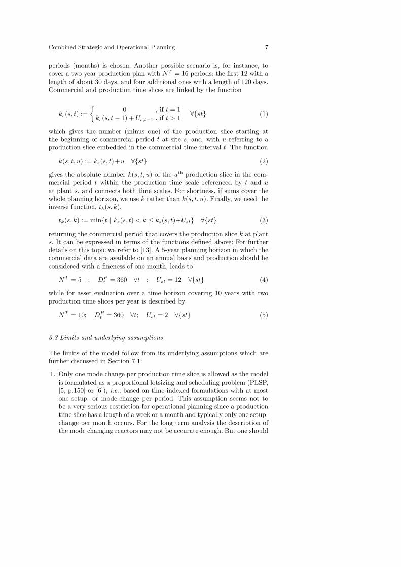
periods (months) is chosen. Another possible scenario is, for instance, tocover a two year production plan with NT = 16 periods: the first 12 with alength of about 30 days, and four additional ones with a length of 120 days.Commercial and production time slices are linked by the function
ks(s, t) :={
0 , if t = 1ks(s, t− 1) + Us,t−1 , if t > 1 ∀{st} (1)
which gives the number (minus one) of the production slice starting atthe beginning of commercial period t at site s, and, with u referring to aproduction slice embedded in the commercial time interval t. The function
k(s, t, u) := ks(s, t)+u ∀{st} (2)
gives the absolute number k(s, t, u) of the uth production slice in the com-mercial period t within the production time scale referenced by t and uat plant s, and connects both time scales. For shortness, if sums cover thewhole planning horizon, we use k rather than k(s, t, u). Finally, we need theinverse function, tk(s, k),
tk(s, k) := min{t | ks(s, t) < k ≤ ks(s, t)+Ust} ∀{st} (3)
returning the commercial period that covers the production slice k at plants. It can be expressed in terms of the functions defined above: For furtherdetails on this topic we refer to [13]. A 5-year planning horizon in which thecommercial data are available on an annual basis and production should beconsidered with a fineness of one month, leads to
NT = 5 ; DPt = 360 ∀t ; Ust = 12 ∀{st} (4)
while for asset evaluation over a time horizon covering 10 years with twoproduction time slices per year is described by
NT = 10; DPt = 360 ∀t; Ust = 2 ∀{st} (5)
3.3 Limits and underlying assumptions
The limits of the model follow from its underlying assumptions which arefurther discussed in Section 7.1:
1. Only one mode change per production time slice is allowed as the modelis formulated as a proportional lotsizing and scheduling problem (PLSP,[5, p.150] or [6]), i.e., based on time-indexed formulations with at mostone setup- or mode-change per period. This assumption seems not tobe a very serious restriction for operational planning since a productiontime slice has a length of a week or a month and typically only one setup-change per month occurs. For the long term analysis the description ofthe mode changing reactors may not be accurate enough. But one should
8 Josef Kallrath
keep in mind that the demand forecast and other input data are oflimited accuracy as well; the client regarded the approach as sufficientlyaccurate and realistic.
2. Transport times are of the order of a few days. In the 12-month scenariostransport times are only considered using a probability assumption. Ineven longer term scenarios transport times are neglected.
3. Only variable inventory costs are considered. They are based on thecapital tied up in inventories and interest rates.
4. Design reactors cannot be subject to intrinsic mode changes. In thecurrent case this limitation did not cause any problems because theapproximately 30 reactors subject to design decisions were single productreactors.
5. Production utilization rates and associated constraints refer to utiliza-tion per production slice. At present, the model does not include con-straints enforcing global utilization aspects of the supply network.
6. In order to support net present value considerations all cost related dataare discounted over time using a discount rate of p%.
4 The mathematical model: the operational planning aspects
4.1 Plants, reactors and production
Each plant consists of one or two sets of reactors. While all reactors aresubject to multi-stage production requirements and possible coproduction,some are multi-purpose reactors subject to mode changes. Topologically,at each plant, the reactors are arranged in chains, in which each reactorneeds only one pre-product; however, the current model formulation doesnot exploit this features and can also be applied to convergent or divergentmaterial flows and more general topologies. The reactors within a chainoperate simultaneously and at different levels of the multi-stage productionprocess. There exist capacity limits for each reactor and task, as well ascapacities for the production of each product, and minimum productionrequirements. Some reactors in the chain are subject to mode changes lastingusually one or two days. Reactors obtain products from preceding reactorsor from tanks, and charge the products through pipelines to tanks or tosubsequent reactors.
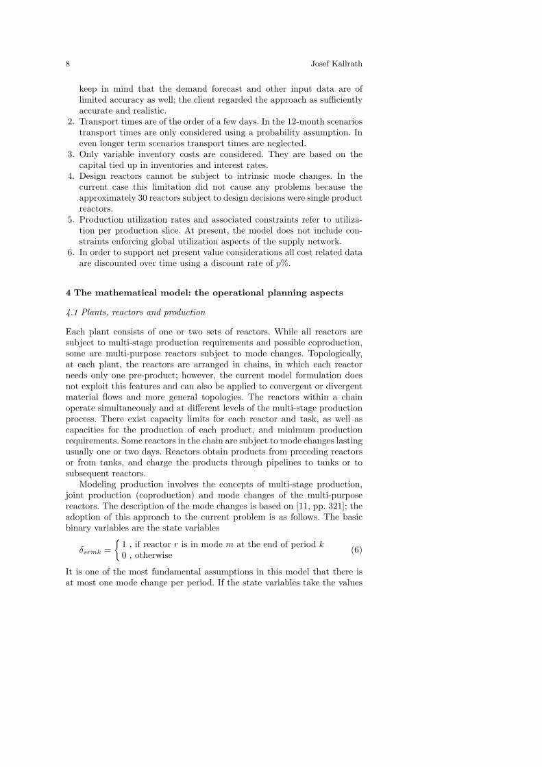
Modeling production involves the concepts of multi-stage production,joint production (coproduction) and mode changes of the multi-purposereactors. The description of the mode changes is based on [11, pp. 321]; theadoption of this approach to the current problem is as follows. The basicbinary variables are the state variables
δsrmk ={
1 , if reactor r is in mode m at the end of period k0 , otherwise (6)
It is one of the most fundamental assumptions in this model that there isat most one mode change per period. If the state variables take the values
Combined Strategic and Operational Planning 9
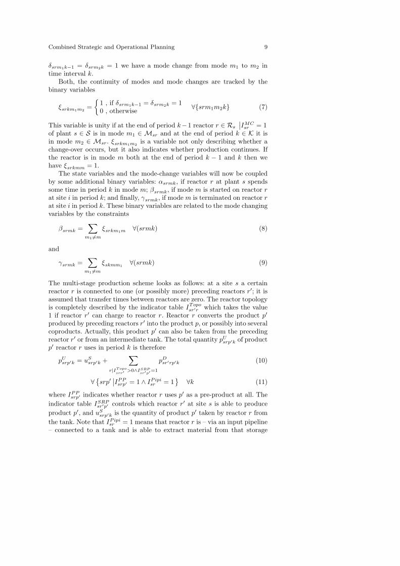
δsrm1k−1 = δsrm2k = 1 we have a mode change from mode m1 to m2 intime interval k.
Both, the continuity of modes and mode changes are tracked by thebinary variables
ξsrkm1m2=
{1 , if δsrm1k−1 = δsrm2k = 10 , otherwise ∀{srm1m2k} (7)
This variable is unity if at the end of period k−1 reactor r ∈ Rs
∣∣IMCsr = 1
of plant s ∈ S is in mode m1 ∈ Msr and at the end of period k ∈ K it isin mode m2 ∈ Msr. ξsrkm1m2
is a variable not only describing whether achange-over occurs, but it also indicates whether production continues. Ifthe reactor is in mode m both at the end of period k − 1 and k then wehave ξsrkmm = 1.
The state variables and the mode-change variables will now be coupledby some additional binary variables: αsrmk, if reactor r at plant s spendssome time in period k in mode m; βsrmk, if mode m is started on reactor rat site i in period k; and finally, γsrmk, if mode m is terminated on reactor rat site i in period k. These binary variables are related to the mode changingvariables by the constraints
βsrmk =∑
m1 6=m
ξsrkm1m ∀(srmk) (8)
and
γsrmk =∑
m1 6=m
ξskmm1∀(srmk) (9)
The multi-stage production scheme looks as follows: at a site s a certainreactor r is connected to one (or possibly more) preceding reactors r′; it isassumed that transfer times between reactors are zero. The reactor topologyis completely described by the indicator table ITopo
sr′r which takes the value1 if reactor r′ can charge to reactor r. Reactor r converts the product p′
produced by preceding reactors r′ into the product p, or possibly into severalcoproducts. Actually, this product p′ can also be taken from the precedingreactor r′ or from an intermediate tank. The total quantity pU
srp′k of productp′ reactor r uses in period k is therefore
pUsrp′k = uS
srp′k +∑
r|IT opo
srr′ >0∧ISRPsr′p′=1
pDsr′rp′k (10)
∀{srp′
∣∣IPPsrp′ = 1 ∧ IPipi
sr = 1}
∀k (11)
where IPPsrp′ indicates whether reactor r uses p′ as a pre-product at all. The
indicator table ISRPsr′p′ controls which reactor r′ at site s is able to produce
product p′, and uSsrp′k is the quantity of product p′ taken by reactor r from
the tank. Note that IPipisr = 1 means that reactor r is – via an input pipeline
– connected to a tank and is able to extract material from that storage
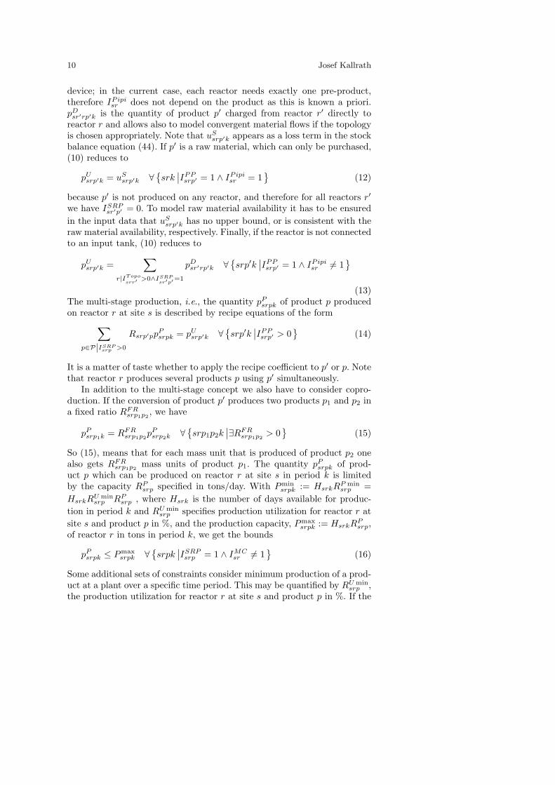
10 Josef Kallrath
device; in the current case, each reactor needs exactly one pre-product,therefore IPipi
sr does not depend on the product as this is known a priori.pD
sr′rp′k is the quantity of product p′ charged from reactor r′ directly toreactor r and allows also to model convergent material flows if the topologyis chosen appropriately. Note that uS
srp′k appears as a loss term in the stockbalance equation (44). If p′ is a raw material, which can only be purchased,(10) reduces to
pUsrp′k = uS
srp′k ∀{srk
∣∣IPPsrp′ = 1 ∧ IPipi
sr = 1}
(12)
because p′ is not produced on any reactor, and therefore for all reactors r′
we have ISRPsr′p′ = 0. To model raw material availability it has to be ensured
in the input data that uSsrp′k has no upper bound, or is consistent with the
raw material availability, respectively. Finally, if the reactor is not connectedto an input tank, (10) reduces to
pUsrp′k =
∑r|IT opo
srr′ >0∧ISRPsr′p′=1
pDsr′rp′k ∀
{srp′k
∣∣IPPsrp′ = 1 ∧ IPipi
sr 6= 1}
(13)The multi-stage production, i.e., the quantity pP
srpk of product p producedon reactor r at site s is described by recipe equations of the form∑
p∈P|ISRPsrp >0
Rsrp′ppPsrpk = pU
srp′k ∀{srp′k
∣∣IPPsrp′ > 0
}(14)
It is a matter of taste whether to apply the recipe coefficient to p′ or p. Notethat reactor r produces several products p using p′ simultaneously.
In addition to the multi-stage concept we also have to consider copro-duction. If the conversion of product p′ produces two products p1 and p2 ina fixed ratio RFR
srp1p2, we have
pPsrp1k = RFR
srp1p2pP
srp2k ∀{srp1p2k
∣∣∃RFRsrp1p2
> 0}
(15)
So (15), means that for each mass unit that is produced of product p2 onealso gets RFR
srp1p2mass units of product p1. The quantity pP
srpk of prod-uct p which can be produced on reactor r at site s in period k is limitedby the capacity RP
srp specified in tons/day. With Pminsrpk := HsrkRP min
srp =HsrkRU min
srp RPsrp , where Hsrk is the number of days available for produc-
tion in period k and RU minsrp specifies production utilization for reactor r at
site s and product p in %, and the production capacity, Pmaxsrpk := HsrkRP
srp,of reactor r in tons in period k, we get the bounds
pPsrpk ≤ Pmax
srpk ∀{srpk
∣∣ISRPsrp = 1 ∧ IMC
sr 6= 1}
(16)
Some additional sets of constraints consider minimum production of a prod-uct at a plant over a specific time period. This may be quantified by RU min
srp ,the production utilization for reactor r at site s and product p in %. If the
Combined Strategic and Operational Planning 11
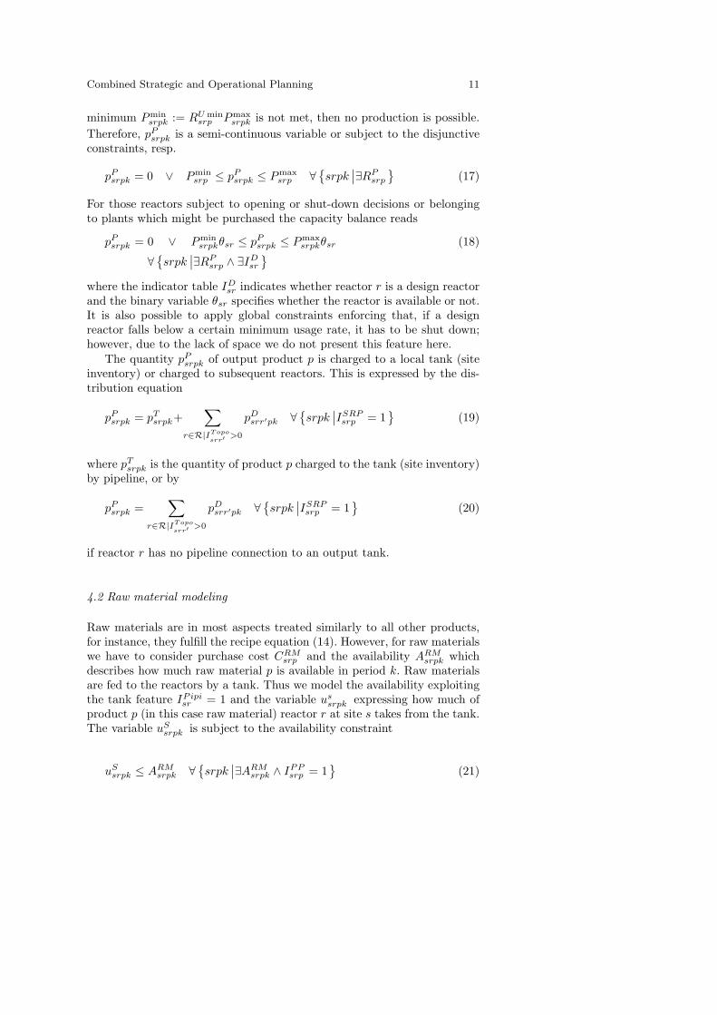
minimum Pminsrpk := RU min
srp Pmaxsrpk is not met, then no production is possible.
Therefore, pPsrpk is a semi-continuous variable or subject to the disjunctive
constraints, resp.
pPsrpk = 0 ∨ Pmin
srp ≤ pPsrpk ≤ Pmax
srp ∀{srpk
∣∣∃RPsrp
}(17)
For those reactors subject to opening or shut-down decisions or belongingto plants which might be purchased the capacity balance reads
pPsrpk = 0 ∨ Pmin
srpkθsr ≤ pPsrpk ≤ Pmax
srpkθsr (18)
∀{srpk
∣∣∃RPsrp ∧ ∃ID
sr
}where the indicator table ID
sr indicates whether reactor r is a design reactorand the binary variable θsr specifies whether the reactor is available or not.It is also possible to apply global constraints enforcing that, if a designreactor falls below a certain minimum usage rate, it has to be shut down;however, due to the lack of space we do not present this feature here.
The quantity pPsrpk of output product p is charged to a local tank (site
inventory) or charged to subsequent reactors. This is expressed by the dis-tribution equation
pPsrpk = pT
srpk+∑
r∈R|IT opo
srr′ >0
pDsrr′pk ∀
{srpk
∣∣ISRPsrp = 1
}(19)
where pTsrpk is the quantity of product p charged to the tank (site inventory)
by pipeline, or by
pPsrpk =
∑r∈R|IT opo
srr′ >0
pDsrr′pk ∀
{srpk
∣∣ISRPsrp = 1
}(20)
if reactor r has no pipeline connection to an output tank.
4.2 Raw material modeling
Raw materials are in most aspects treated similarly to all other products,for instance, they fulfill the recipe equation (14). However, for raw materialswe have to consider purchase cost CRM
srp and the availability ARMsrpk which
describes how much raw material p is available in period k. Raw materialsare fed to the reactors by a tank. Thus we model the availability exploitingthe tank feature IPipi
sr = 1 and the variable ussrpk expressing how much of
product p (in this case raw material) reactor r at site s takes from the tank.The variable uS
srpk is subject to the availability constraint
uSsrpk ≤ ARM
srpk ∀{srpk
∣∣∃ARMsrpk ∧ IPP
srp = 1}
(21)
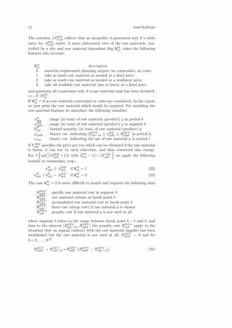
12 Josef Kallrath
The notation ∃ARMsrpk reflects that an inequality is generated only if a table
entry for ARMsrpk exists. A more elaborated view of the raw materials, con-
trolled by a site and raw material dependent flag RMsp , takes the following
features into account:
RMsp description0 material requirement planning output; no constraints, no costs1 take as much raw material as needed at a fixed price2 take as much raw material as needed at a nonlinear price3 take all available raw material (use or burn) at a fixed price
and generates all constraints only if a raw material tank has been declared,i.e., if ∃SSC
sp .If RM
sp = 0 no raw material constraints or costs are considered. In the reportwe just print the raw material which would be required. For modeling theraw material features we introduce the following variables:
uRspk : usage (in tons) of raw material (product) p in period k
uRBspbk : usage (in tons) of raw material (product) p in segment b
bRspk : burned quantity (in tons) of raw material (product) p
µspbk : binary var. indicating RBPVspb−1k ≤ uRB
spbk ≤ RBPVspbk in period k,
ωspt : binary var. indicating the use of raw material p in period t
If Y RMspk specifies the price per ton which can be obtained if the raw material
is burnt, it can not be used otherwise, and thus converted into energy.For ∀
{spk
∣∣∣∃ARMspk ∧
(∃r with IPP
srp = 1)∧ ∃Y RM
spk
}we apply the following
bounds or constraints, resp.:
uRspk ≤ ARM
spk if RMsp = 1 (22)
uRspk + bR
spk = ARMspk if RM
sp = 3 (23)
The case RMsp = 2 is more difficult to model and requires the following data
RBPCspbk specific raw material cost in segment b
RBPVspbk raw material volume at break point b
RACCspbk accumulated raw material cost at break point b
RFIXspk fixed cost (setup cost) if raw material p is chosen
RPENspk penalty cost if raw material p is not used at all
where segment b refers to the range between break point b − 1 and b, andthus to the interval [RBPV
spb−1k, RBPVspbk ] the penalty cost RPEN
spk apply to thesituation that an annual contract with the raw material supplier has beenestablished but the raw material is not used at all, RACC
sp1k = 0 and forb = 2, . . . , NB
RACCspbk = RACC
spb−1k+RBPCspbk
(RBPV
spbk −RBPVspb−1k
)(24)

Combined Strategic and Operational Planning 13
To select the appropriate segment or interval [RBPVspb−1k, RBPV
spbk ] for the quan-tity of raw material purchased we exploit the binary variable µspbk whichindicates that RBPV
spb−1k ≤ uRBspbk ≤ RBPV
spbk . The constraints
NB+1∑b=1
µspbk = 1 ∀{spk
∣∣∃ARMspk ∧ ∃SSC
sp
}(25)
anduRB
spbk ≥ RBPVspb−1kµspbk ∀
{spk
∣∣∃ARMspk ∧ ∃SSC
sp
}(26)
uRBspbk ≤ RBPV
spbk µspbk ∀{spk
∣∣∃ARMspk ∧ ∃SSC
sp
}(27)
guarantee that uRBspbk falls exactly into one segment. Note that µspNB+1k = 1
is used to indicate that no raw material is used at all.The real quantity uR
spk of used raw material is coupled to the segmentquantity by
uRspk =
NB∑b=1
uRBspbk ∀
{spk
∣∣∃ARMspk ∧ ∃SSC
sp
}(28)
As raw material is purchased on the basis of annual contracts, which mightforce that a certain quantity has to be purchased by the provider, we in-troduce the binary variable ρspt indicating whether any quantity of rawmaterial p is used in the commercial period at all
ρspt ≥ 1−µspNB+1k ∀{sptk
∣∣∃ARMspk ∧ ∃SSC
sp
}(29)
If no raw material is used at all, penalty cost may be applied by the provider.An alternative, and in most cases superior formulation of these raw
material aspects replaces (26) to (28) by
uRspk =
NB∑b=2
RBPVspb−1kµspbk+
NB∑b=1
uRBspbk ∀
{spk
∣∣∃ARMspk ∧ ∃SSC
sp
}(30)
uRBspbk ≤ RBPV
sp1k µspbk ∀{spk
∣∣∃ARMspk ∧ ∃SSC
sp
}(31)
where uRspk has a slightly different meaning now, and
uRBspbk ≤
(RBPV
spbk −RBPVspb−11k
)µspbk ∀
{spk
∣∣∃ARMspk ∧ ∃SSC
sp
}(32)
The variable raw material cost are then given by∑s∈S
∑p∈P
NB∑b=2
NKs∑
k=1
RACCspb−1kµspbk +
∑s∈S
∑p∈P
NB∑b=1
NKs∑
k=1
RBPVspbk uRB
spbk (33)
+∑s∈S
∑p∈P
NT∑t=1
RPENspt +
∑s∈S
∑p∈P
NT∑t=1
(RFIX
spt −RPENspt
)ρspt
A special ordered set approach involving the µspbk variables has been testedas well, but did not turn out to be superior compared to the formulation inwhich the µspbk variables are just binary variables.
14 Josef Kallrath
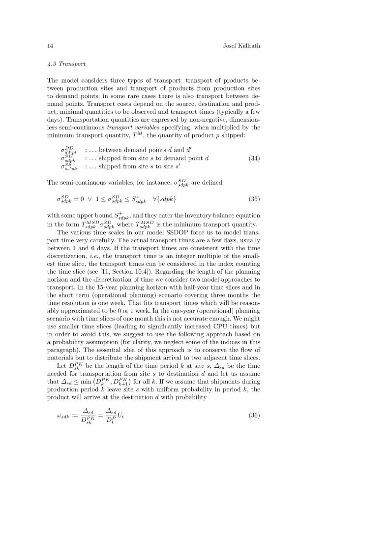
4.3 Transport
The model considers three types of transport: transport of products be-tween production sites and transport of products from production sitesto demand points; in some rare cases there is also transport between de-mand points. Transport costs depend on the source, destination and prod-uct, minimal quantities to be observed and transport times (typically a fewdays). Transportation quantities are expressed by non-negative, dimension-less semi-continuous transport variables specifying, when multiplied by theminimum transport quantity, TM , the quantity of product p shipped:
σDDdd′pt : . . . between demand points d and d′
σSDsdpk : . . . shipped from site s to demand point d
σSSss′pk : . . . shipped from site s to site s′
(34)
The semi-continuous variables, for instance, σSDsdpk are defined
σSDsdpk = 0 ∨ 1 ≤ σSD
sdpk ≤ S+sdpk ∀{sdpk} (35)
with some upper bound S+sdpk, and they enter the inventory balance equation
in the form TMSDsdpk σSD
sdpk where TMSDsdpk is the minimum transport quantity.
The various time scales in our model SSDOP force us to model trans-port time very carefully. The actual transport times are a few days, usuallybetween 1 and 6 days. If the transport times are consistent with the timediscretization, i.e., the transport time is an integer multiple of the small-est time slice, the transport times can be considered in the index countingthe time slice (see [11, Section 10.4]). Regarding the length of the planninghorizon and the discretization of time we consider two model approaches totransport. In the 15-year planning horizon with half-year time slices and inthe short term (operational planning) scenario covering three months thetime resolution is one week. That fits transport times which will be reason-ably approximated to be 0 or 1 week. In the one-year (operational) planningscenario with time slices of one month this is not accurate enough. We mightuse smaller time slices (leading to significantly increased CPU times) butin order to avoid this, we suggest to use the following approach based ona probability assumption (for clarity, we neglect some of the indices in thisparagraph). The essential idea of this approach is to conserve the flow ofmaterials but to distribute the shipment arrival to two adjacent time slices.
Let DPKsk be the length of the time period k at site s, ∆sd be the time
needed for transportation from site s to destination d and let us assumethat ∆sd ≤ min
(DPK
k , DPKk+1
)for all k. If we assume that shipments during
production period k leave site s with uniform probability in period k, theproduct will arrive at the destination d with probability
ωsdk :=∆sd
DPKsk
=∆sd
DPt
Ut (36)
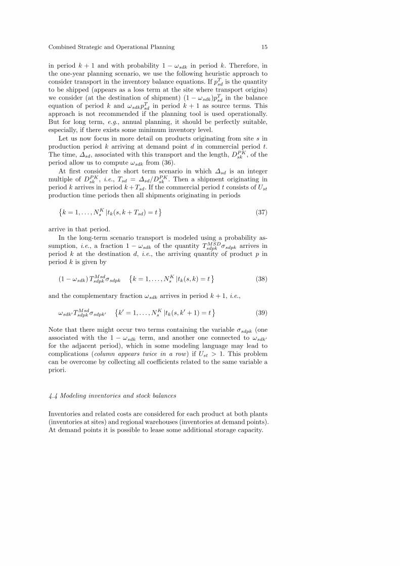
Combined Strategic and Operational Planning 15
in period k + 1 and with probability 1 − ωsdk in period k. Therefore, inthe one-year planning scenario, we use the following heuristic approach toconsider transport in the inventory balance equations. If pT
sd is the quantityto be shipped (appears as a loss term at the site where transport origins)we consider (at the destination of shipment) (1 − ωsdk)pT
sd in the balanceequation of period k and ωsdkpT
sd in period k + 1 as source terms. Thisapproach is not recommended if the planning tool is used operationally.But for long term, e.g., annual planning, it should be perfectly suitable,especially, if there exists some minimum inventory level.
Let us now focus in more detail on products originating from site s inproduction period k arriving at demand point d in commercial period t.The time, ∆sd, associated with this transport and the length, DPK
sk , of theperiod allow us to compute ωsdk from (36).
At first consider the short term scenario in which ∆sd is an integermultiple of DPK
sk , i.e., Tsd = ∆sd/DPKsk . Then a shipment originating in
period k arrives in period k +Tsd. If the commercial period t consists of Ust
production time periods then all shipments originating in periods{k = 1, . . . , NK
s |tk(s, k + Tsd) = t}
(37)
arrive in that period.In the long-term scenario transport is modeled using a probability as-
sumption, i.e., a fraction 1 − ωsdk of the quantity TMSDsdpk σsdpk arrives in
period k at the destination d, i.e., the arriving quantity of product p inperiod k is given by
(1− ωsdk) TMsdsdpk σsdpk
{k = 1, . . . , NK
s |tk(s, k) = t}
(38)
and the complementary fraction ωsdk arrives in period k + 1, i.e.,
ωsdk′TMsdsdpk σsdpk′
{k′ = 1, . . . , NK
s |tk(s, k′ + 1) = t}
(39)
Note that there might occur two terms containing the variable σsdpk (oneassociated with the 1 − ωsdk term, and another one connected to ωsdk′
for the adjacent period), which in some modeling language may lead tocomplications (column appears twice in a row) if Ust > 1. This problemcan be overcome by collecting all coefficients related to the same variable apriori.
4.4 Modeling inventories and stock balances
Inventories and related costs are considered for each product at both plants(inventories at sites) and regional warehouses (inventories at demand points).At demand points it is possible to lease some additional storage capacity.
16 Josef Kallrath
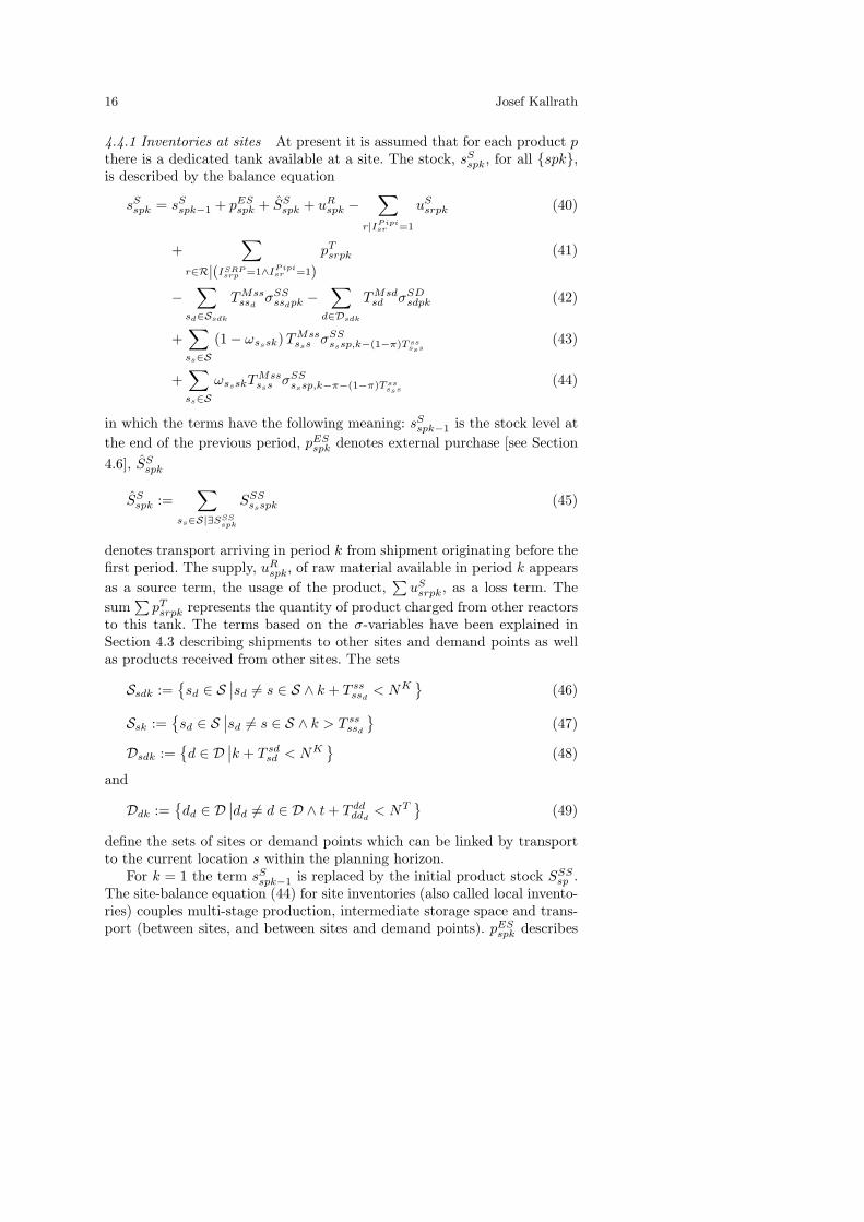
4.4.1 Inventories at sites At present it is assumed that for each product pthere is a dedicated tank available at a site. The stock, sS
spk, for all {spk},is described by the balance equation
sSspk = sS
spk−1 + pESspk + SS
spk + uRspk −
∑r|IP ipi
sr =1
uSsrpk (40)
+∑
r∈R|(ISRPsrp =1∧IP ipi
sr =1)pT
srpk (41)
−∑
sd∈Ssdk
TMssssd
σSSssdpk −
∑d∈Dsdk
TMsdsd σSD
sdpk (42)
+∑ss∈S
(1− ωsssk) TMsssss σSS
sssp,k−(1−π)T sssss
(43)
+∑ss∈S
ωssskTMsssss σSS
sssp,k−π−(1−π)T sssss
(44)
in which the terms have the following meaning: sSspk−1 is the stock level at
the end of the previous period, pESspk denotes external purchase [see Section
4.6], SSspk
SSspk :=
∑ss∈S|∃SSS
spk
SSSssspk (45)
denotes transport arriving in period k from shipment originating before thefirst period. The supply, uR
spk, of raw material available in period k appearsas a source term, the usage of the product,
∑uS
srpk, as a loss term. Thesum
∑pT
srpk represents the quantity of product charged from other reactorsto this tank. The terms based on the σ-variables have been explained inSection 4.3 describing shipments to other sites and demand points as wellas products received from other sites. The sets
Ssdk :={sd ∈ S
∣∣sd 6= s ∈ S ∧ k + T ssssd
< NK}
(46)
Ssk :={sd ∈ S
∣∣sd 6= s ∈ S ∧ k > T ssssd
}(47)
Dsdk :={d ∈ D
∣∣k + T sdsd < NK
}(48)
and
Ddk :={dd ∈ D
∣∣dd 6= d ∈ D ∧ t + T ddddd
< NT}
(49)
define the sets of sites or demand points which can be linked by transportto the current location s within the planning horizon.
For k = 1 the term sSspk−1 is replaced by the initial product stock SSS
sp .The site-balance equation (44) for site inventories (also called local invento-ries) couples multi-stage production, intermediate storage space and trans-port (between sites, and between sites and demand points). pES
spk describes
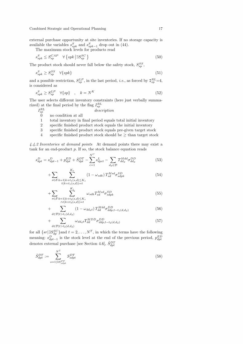
Combined Strategic and Operational Planning 17
external purchase opportunity at site inventories. If no storage capacity isavailable the variables sS
spk and sSspk−1 drop out in (44).
The maximum stock levels for products read
sSspk ≤ SCAP
sp ∀{spk
∣∣∃SSCsp
}(50)
The product stock should never fall below the safety stock, SSSsp ,
sSspk ≥ SSS
sp ∀{spk} (51)
and a possible restriction, SLPsp , in the last period, i.e., as forced by IRL
sp =4,is considered as
sSspk ≥ SLP
sp ∀{sp} , k = NK (52)
The user selects different inventory constraints (here just verbally summa-rized) at the final period by the flag IRL
sp
IRLsp description0 no condition at all1 total inventory in final period equals total initial inventory2 specific finished product stock equals the initial inventory3 specific finished product stock equals pre-given target stock4 specific finished product stock should be ≥ than target stock
4.4.2 Inventories at demand points At demand points there may exist atank for an end-product p. If so, the stock balance equation reads
sDdpt = sD
dpt−1 + pEDdpt + SDT
dpt −NC∑c=1
sLdpct −
∑dd∈D
TMddddd
σDDddd
(53)
+∑s∈S
Ks∑k=1|k+t1(s,d)≤Ks
t(k+t1(s,d))=t
(1− ωsdk) TMsdsd σSD
sdpk (54)
+∑s∈S
Ks∑k=1|k+t2(s,d)≤Ks
∧t(k+t2(s,d))=t
ωsdkTMsdsd σSD
sdpk (55)
+∑
d∈D|t>t1(d,dd)
(1− ωdddt)TMdddd σDD
ddp,t−t1(d,dd) (56)
+∑
d∈D|t>t2(d,dd)
ωdddtTMDDdd σDD
ddp,t−t2(d,dd) (57)
for all {sr|∃SSCdp }and t = 2, . . . , NT , in which the terms have the following
meaning: sDdpt−1 is the stock level at the end of the previous period, pED
dpt
denotes external purchase [see Section 4.6], SDTdpt
SDTdpt :=
NS∑s=1|∃SP T
sdpt
SDTsdpt (58)
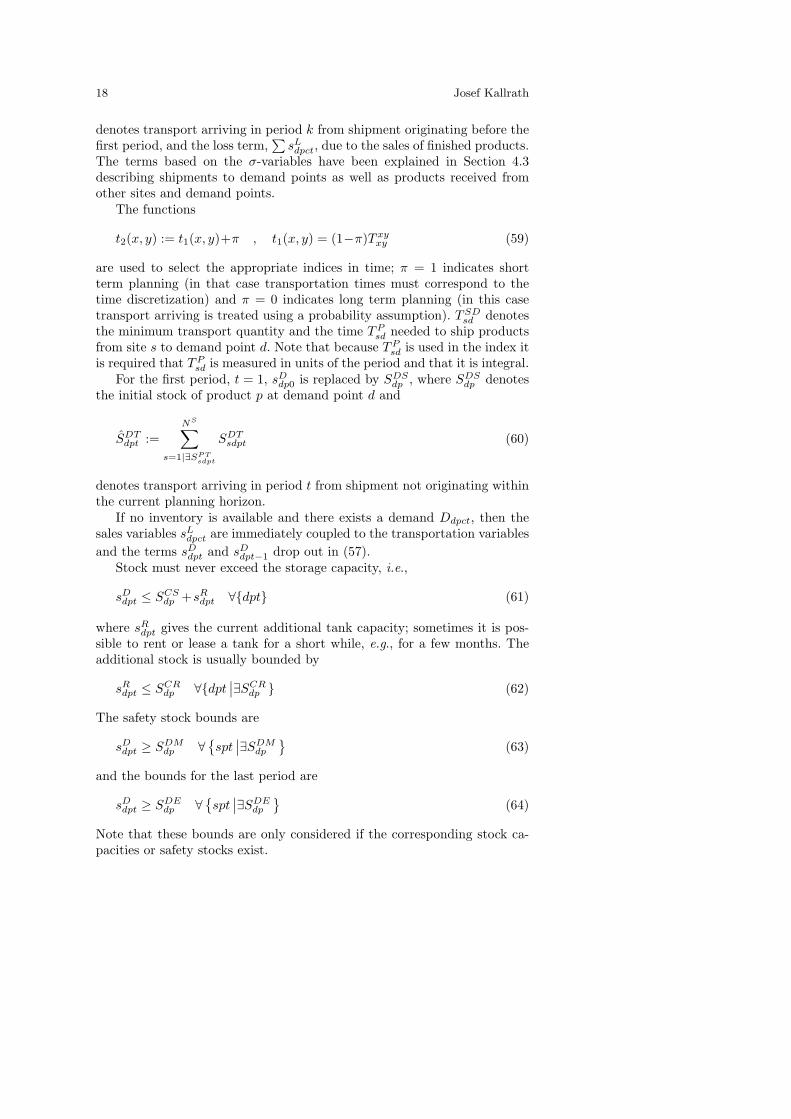
18 Josef Kallrath
denotes transport arriving in period k from shipment originating before thefirst period, and the loss term,
∑sL
dpct, due to the sales of finished products.The terms based on the σ-variables have been explained in Section 4.3describing shipments to demand points as well as products received fromother sites and demand points.
The functions
t2(x, y) := t1(x, y)+π , t1(x, y) = (1−π)T xyxy (59)
are used to select the appropriate indices in time; π = 1 indicates shortterm planning (in that case transportation times must correspond to thetime discretization) and π = 0 indicates long term planning (in this casetransport arriving is treated using a probability assumption). TSD
sd denotesthe minimum transport quantity and the time TP
sd needed to ship productsfrom site s to demand point d. Note that because TP
sd is used in the index itis required that TP
sd is measured in units of the period and that it is integral.For the first period, t = 1, sD
dp0 is replaced by SDSdp , where SDS
dp denotesthe initial stock of product p at demand point d and
SDTdpt :=
NS∑s=1|∃SP T
sdpt
SDTsdpt (60)
denotes transport arriving in period t from shipment not originating withinthe current planning horizon.
If no inventory is available and there exists a demand Ddpct, then thesales variables sL
dpct are immediately coupled to the transportation variablesand the terms sD
dpt and sDdpt−1 drop out in (57).
Stock must never exceed the storage capacity, i.e.,
sDdpt ≤ SCS
dp +sRdpt ∀{dpt} (61)
where sRdpt gives the current additional tank capacity; sometimes it is pos-
sible to rent or lease a tank for a short while, e.g., for a few months. Theadditional stock is usually bounded by
sRdpt ≤ SCR
dp ∀{dpt∣∣∃SCR
dp } (62)
The safety stock bounds are
sDdpt ≥ SDM
dp ∀{spt
∣∣∃SDMdp
}(63)
and the bounds for the last period are
sDdpt ≥ SDE
dp ∀{spt
∣∣∃SDEdp
}(64)
Note that these bounds are only considered if the corresponding stock ca-pacities or safety stocks exist.
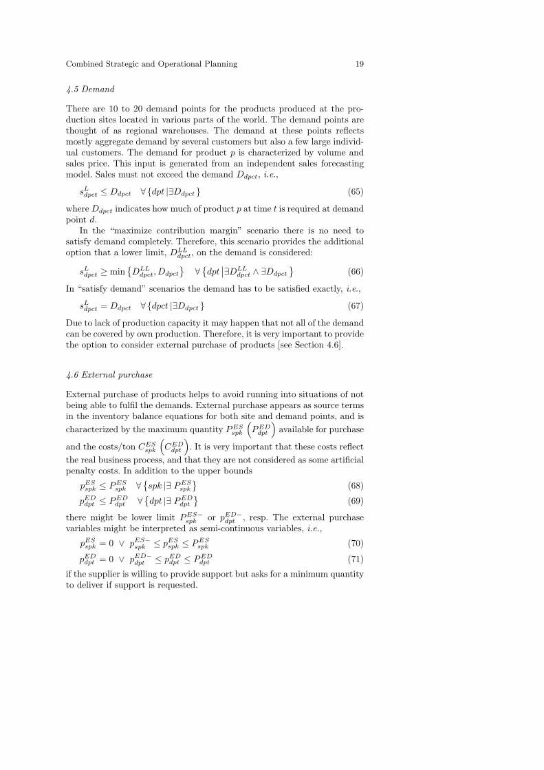
Combined Strategic and Operational Planning 19
4.5 Demand
There are 10 to 20 demand points for the products produced at the pro-duction sites located in various parts of the world. The demand points arethought of as regional warehouses. The demand at these points reflectsmostly aggregate demand by several customers but also a few large individ-ual customers. The demand for product p is characterized by volume andsales price. This input is generated from an independent sales forecastingmodel. Sales must not exceed the demand Ddpct, i.e.,
sLdpct ≤ Ddpct ∀ {dpt |∃Ddpct } (65)
where Ddpct indicates how much of product p at time t is required at demandpoint d.
In the “maximize contribution margin” scenario there is no need tosatisfy demand completely. Therefore, this scenario provides the additionaloption that a lower limit, DLL
dpct, on the demand is considered:
sLdpct ≥ min
{DLL
dpct, Ddpct
}∀
{dpt
∣∣∃DLLdpct ∧ ∃Ddpct
}(66)
In “satisfy demand” scenarios the demand has to be satisfied exactly, i.e.,
sLdpct = Ddpct ∀ {dpct |∃Ddpct } (67)
Due to lack of production capacity it may happen that not all of the demandcan be covered by own production. Therefore, it is very important to providethe option to consider external purchase of products [see Section 4.6].
4.6 External purchase
External purchase of products helps to avoid running into situations of notbeing able to fulfil the demands. External purchase appears as source termsin the inventory balance equations for both site and demand points, and ischaracterized by the maximum quantity PES
spk
(PED
dpt
)available for purchase
and the costs/ton CESspk
(CED
dpt
). It is very important that these costs reflect
the real business process, and that they are not considered as some artificialpenalty costs. In addition to the upper bounds
pESspk ≤ PES
spk ∀{spk |∃ PES
spk
}(68)
pEDdpt ≤ PED
dpt ∀{dpt |∃ PED
dpt
}(69)
there might be lower limit PES−spk or pED−
dpt , resp. The external purchasevariables might be interpreted as semi-continuous variables, i.e.,
pESspk = 0 ∨ pES−
spk ≤ pESspk ≤ PES
spk (70)
pEDdpt = 0 ∨ pED−
dpt ≤ pEDdpt ≤ PED
dpt (71)
if the supplier is willing to provide support but asks for a minimum quantityto deliver if support is requested.
20 Josef Kallrath
5 The mathematical model: the design decisions
Since the network consists of several plants with different product streamsit seems adequate to investigate whether it makes sense
– to open certain reactors at a site and to produce additional products,– to shut-down certain reactors and thus not to produce some products at
this site,– or to buy whole sites.
One way to analyze such questions is to run different scenarios and to pickthe best one. This simulation approach, however, might fail to identify thereal good candidates and the optimal solution. The alternative approach isto model these questions or corresponding features appropriately and letthe optimizer come up with optimal suggestions regarding the design of theproduction network.
5.1 A simple approach to include design decisions
A simple inclusion of the design features realized in the first phase of theproject was to let the optimizer choose whether to open or shutdown areactor once and for ever at the beginning of the planning horizon. Thatapproach involves the following data: the total cost for buying a plant, CB
s ,the annual cost for buying a plant, CBA
s , the fixed cost to operate a reactor,CFIX
sr , the event value cost to open a reactor, COsr, and the event value
cost to shut down a reactor, CSDsr . The design costs to be included in a
net profit objective function (contribution margin minus fixed costs minusdesign costs) has the form
−zD : =∑
s∈S|∃CBAs
CBAs ηs +
∑s∈S
∑r∈R|∃CSDA
sr
(CSDA
sr − CFIXsr
)ϕsr
+∑s∈S
∑r∈R|∃CSO
sr
(CO
sr + CFIXsr
)µsr (72)
where the binary variables ηs, ϕsr and µsr indicate whether a plant isbought, a reactor is shut down or opened.
An additional binary variable θsr is introduced if IDsr = 1;
IDsr = 1 ⇔
{IsRsr = 1 ∧
(∃CBA
s ∨ CSDsr ∨ CO
sr
)}(73)
where IDsr indicates whether reactor r at site s is subject to design decisions;
most cases we studied involved about 30 design reactors. θsr controls theavailable capacity of a reactor and is related to the other binary variablesas follows:
θsr = ηs ∀{sr |∃ IsR
sr = 1 ∧ ∃CBAs
}(74)
θsr = 1−ϕsr ∀{sr |∃ IsR
sr = 1 ∧ ∃CSDsr
}(75)
Combined Strategic and Operational Planning 21
θsr = µsr ∀{sr |∃ IsR
sr = 1 ∧ ∃COsr
}(76)
The relations (74) to (76) give us a hint on possible priorities (ηs,ϕsr,µsr,θsr)for the variables in the branching process. It is assumed that CSD
sr and COsr
do not exist simultaneously.The disadvantage of that approach, in a 10- or 15-year planning horizon,
is that a reactor has to be opened or shut down in the first period of theplanning horizon and stays in that status for the rest of the planning horizon.A more detailed view described in the next section allows for time dependentand temporary shutdowns and openings.
5.2 Time dependent and temporary shutdowns
In the course of the project it became obvious that more details regard-ing time resolution are necessary. Therefore, reactors, for which opening orshutdown cost are specified, will be treated as reactors subject to time de-pendent opening or shutdown decisions. These reactors are modeled similaras the reactors subject to mode changes. For each design reactor we assigntwo modes (m = 1 and 2 corresponding to on and off ), and use the variablesαsr1k , βsr1k, γsr1k, and δsr1k explained in ([11, Section 10.4]). Note thatthis model approach implies that the design reactors can not be subject tointrinsic mode changes which was not a problem in the current application.However, it is now possible that both CSD
srk and COsrk may be different from
zero. A further detail to be considered is that the opening decisions needsome time to be put into reality. Therefore, a delay time KFO
sr might specifywhich production time slice is the first one in which the reactor could beopened. This conditions, for k = 1, . . . ,max(1,KFO
sr − 1), is realized by thebounds
αsr1k = βsr1k = δsr1k = 0 ∀(sr) ∈ RD := {(sr)∣∣IMC
sr 6= 1 ∧ ∃IIBRsr }
(77)for all design reactors which are not yet opened.
Although, the economical parameters may already prevent that reactorsare opened and shut down wildly and very frequently it might be necessaryfor managerial reasons to introduce two parameters, KO and KC , whichspecify that if a reactor is opened in production time slice k, it has to beopen for the next KO time slices, and vice versa, if a reactor is shutdown inperiod k it has to stay closed for the next KC time slices. These conditionstighten the model constraints by putting the variables αsr1k, βsr1k, γsr1k
and δsr1k to zero for certain time slices in which a plant cannot operate andare enforced by
k+KO∑κ=k+1
γsr1k ≤ KO−KOβsr1k ∀(sr) ∈ RD, ∀k ∈ KOs (78)
k+KC∑κ=k+1
αsr1k ≤ KC−KCγsr1k ∀(sr) ∈ RD, ∀k ∈ KCs (79)
22 Josef Kallrath
k+KC∑κ=k+1
βsr1k ≤ KC−KCγsr1k ∀(sr) ∈ RD, ∀k ∈ KCs (80)
k+KC∑κ=k+1
δsr1k ≤ KC−KCγsr1k ∀(sr) ∈ RD, ∀k ∈ KCs (81)
k+KO∑κ=k+1
δsr1k ≥ (KO−1)βsr1k ∀(sr) ∈ RD, ∀k ∈ KOs (82)
k+KC∑κ=k+1
γsr1k ≤ KC−KCγsr1k ∀(sr) ∈ RD, ∀k ∈ KCs (83)
k+KC∑κ=k+1
βsr1k ≤ KO−KOβsr1k ∀(sr) ∈ RD, ∀k ∈ KOs (84)
withKCs := {1, . . . ,max(1, NK(s)−KC)} andKO
s := {1, . . . ,max(1, NK(s)−KO)}. Finally, when a reactor is open, i.e., αsr1k = 1, it is ensured that acertain minimum quantity is really produced, i.e.,
pPsrpk ≥ PMIN
srpk αsr1k ∀{srpk
∣∣IMCsr 6= 1 ∧ ∃IIBR
sr ∧ ∃ISRPsrp
}(85)
Note that (85) cannot be applied to reactors which are design reactors andare already open at the beginning of the planning horizon. The reason is thatfor such reactors we necessarily have αsr1k = 1. However, if such a reactoris subject to a shutdown decision it may be not even able to produce andthus cannot meet the minimum production requirement (85).
The basic cost terms are the costs for shutdown and opening adjustedfor discounted cash flows and depreciation (see below), i.e., terms such as
cD1 :=∑
(sr)∈RD
NKs∑
k=1
CSDsrkγsr1k , cD2 :=
∑(sr)∈RD
NKs∑
k=1
COsrkβsr1k (86)
The improved design model also considers the residual book value Vsrk [seeEquation (90)] of an opened reactor, i.e., a reactor which caused openingcost) at the end of the planning horizon. This adds the term
zD2 := −∑
{sr}∈RD
NKs∑
k=1
Vsrkβsr1k+∑
{sr}∈RD
NKs∑
k=1
Vsrkγsr1k (87)
to the objective function. Vsrk is based on the net present value and on thedepreciation. At present we apply a linear depreciation rate. The discountedopening cost in production time slice k are DP
t /Ust
COsrk = CO
sr/Dk−1 , D := 1+p
100Ust(88)
Combined Strategic and Operational Planning 23
where p is the discount rate in percent. The calculation of the depreciationdepends on the opening time and thus we obtain the depreciation factor
FDs := 1− NK
s − k
UstTD(89)
where TD denotes the depreciation time in years; a typical value is TD = 15years. Formula (89) for the computation of the depreciation factor assumesthat the depreciation time is measured in units of the commercial time scale;typically the discretization of the commercial time periods is one year andso the depreciation time is also given in years. Based on these assumptions,if the opening occurs in period k the residual book value is
Vsrk = COsr/Dk−1
(1− NK
s − k
UstTD
)(90)
If we assume that a reactor which causes opening cost is not shut down,i.e., it is opened at most once, the term added to the objective function is
∑{sr}∈RD
NKs∑
k=1
Vsrkαsr1NKs
βsr1k =∑
{sr}∈RD
NKs∑
k=1
Vsrkβsr1k (91)
Therefore, the total contribution of βsr1k to the design term in the objectivefunction representing the opening cost and the residual book value is
zD2 :=∑
{sr}∈RD
NKs∑
k=1
(Vsrk − CO
srk
)βsr1k (92)
An additional cost term is included to describe reactors that are subject toa shutdown decision in the first period but require continuation cost CCNT
sr ,e.g., for maintaining or upgrading existing facilities, if the reactor is not shutdown in the first period. This feature is considered by the binary variable
σsr ∀{sr
∣∣(sr) ∈ RD ∧ ∃CCNTsr
}(93)
the constraint
σsr ≥ 1−γsr11 ∀{sr
∣∣(sr) ∈ RD ∧ ∃CCNTsr
}(94)
and the costs term
cD3 :=∑
(sr)∈RD|∃CCNTsr
CCNTsr σsr (95)
in the net profit objective function.The total contribution of the design reactors to the objective function is
zD := −cD1 +zD2−cD3 (96)
24 Josef Kallrath
6 The mathematical model: the objective functions
The model covers eight different objective functions invoked by OBJTYPE=n,where n is a number between 1 and 8:
1. “max. contribution margin” ([11, Section 10.4])2. “max. contribution margin while guaranteeing minimum demand”3. “min. cost while satisfying full demand” ([13])4. “max. total sales neglecting cost” ([13])5. “max. net profit” (the detailed and full design problem)6. “multi-criteria objectives” (maximize profit & minimize transport)7. “max. total production”8. “max. total production of products for which demand exists”
Only the fifth one exploits all design features; all other assume a fixed de-sign. The first one maximizes the contribution margin, y − c, and includesthe yield, y, calculated on the basis of production and the associated salesprices and the sum of all variable cost c. The second one minimizes thevariable cost, c, while satisfying demand. In the cases 1 to 6 the follow-ing variable cost are involved: variable production cost, change-over cost,transport between sites, between sites and demand points, and between de-mand points, inventory cost for products, and cost for external purchase ofproducts; in case 5 these cost terms are discounted according to Section 5.2which leads to the net profit objective function
max z , z := y−c+zD (97)
The objective functions 7 and 8 are used in an initial phase to test thedata and to derive the theoretical capacity of the production network. Thetotal net profit objective function contain the design cost terms which havequite different scaling characteristics compared to the standard productionplanning terms. Using variable directives in the B&B scheme, i.e., priori-tizing the design decisions, it was possible to cope with this problem. Themulti-criteria objectives scenario is solved by a goal programming approachas described in [9].
7 Computational issues, implementation and results
The model has been coded and the MILP problem has been solved usingDash’s modeling language and MILP-solver XPRESS-MP 10.60 ([2], [3] and[4]). During some first numerical experiments it was observed that the ob-jective function in the scenarios 4, 7 and 8 was dually degenerated. Thus,a significant speed-up was achieved using the primal Simplex algorithm tosolve these scenarios. Some DOS-based procedures have been programmedto automate the process of accessing the data from an EXCEL spreadsheet,generating the matrix, solving the problem and returning the results intothe EXCEL spreadsheet. Especially, some batch files developed enabled us topass appropriate command streams to the solver depending on the objectivefunction scenario.
Combined Strategic and Operational Planning 25
7.1 Model assumptions and validation
The first step of model validation was to review and summarize the assump-tions and limitations of our mathematical model. They are already givenin Section 3.3 but in this practical case, only the implementation of themodel showed that they have been reasonable and acceptable. The modelwas carefully validated by the client, i.e., by an experienced productionplanner and a financial expert running the model and the software underdifferent circumstances. Especially, the opening and shut-down of reactorswere carefully traced and subject to plausibility checks by the financial plan-ners, for instance, taking into account the contribution margin related to anewly opened reactor compared to its investment cost. It was interesting toinspect solutions in which a reactor which was no longer profitable was shut-down immediately, after a reactor based on a new technology was opened.Transport between sites and demand points was an issue which sometimeslead to solutions non-intuitive to the people responsible for the productionplanning in single plants, and usually needed clarification.
7.2 Computational issues
To give an example of the problem size and some solution characteristics wequote a typical scenario (S5) with about 30 design reactors covering 10 yearswith 10 commercial and 20 production time slices, for which we derived pro-duction and design plans maximizing total net profit. Using Dash’s MILP-solver XPRESS-MP 10.60 ([2], [3] and [4]) for a problem with nc = 26941continuous, nc = 5100 binary and nsc = 1100 semi-continuous variablesand c = 28547 constraints, we got the following results (including the in-teger solution number IP , number of nodes nn, run time τ on a 266 MHzPentium II PC in minutes, best upper bound zU , best lower bound zL andintegrality gap ∆ := 100 zU−zL
zL ):
IP nn τ zU zL ∆S5 1 218 4 140.8 137.5 2.4S5 2 1794 34 138.4 138.4 −
The first feasible integer solution is usually found within 10 minutes afterexploring about 300 nodes in the B&B tree. Usually, for pure operationalplanning, this solution is accepted and the tree search is terminated. Thisheuristic is justified if ∆ is of the order of a few percent (well within theerror associated with the input data) because it eliminates the need for thetime consuming complete search for the absolute optimal solution via theB&B algorithm. In the SSDOP approach this is only valid, if ∆ is less orequal, say, 1%.
It is remarkable that this model even when all design features are ex-ploited is able to find the first feasible integer solution, usually after 200 or
26 Josef Kallrath
300 nodes, within a few minutes (integrality gap between 1 and 3 percent)and is able to prove optimality in most cases within 30 minutes (3000 nodestypically). If all design features are fixed, the problem is solved to optimalitywithin a few minutes (1000 to 2000 nodes).
In order to carry out sensitivity analyses of the solution with respectto the input data, especially to the demand data and costs or sales prices,it is important that we are able to conduct the complete search via theB&B algorithm or to get an integrality gap ∆ less than one percent. Thesensitivity analysis was carried out by the client by varying the input databy up to 20 percent and inspecting the objective function value and thedesign decisions.
7.3 Commercial results, benefits and experience
The client reports cost savings of several millions of US$. These cost sav-ings were achieved via a reduction in transportation cost compared to theprevious year when the model was not in use. The solution for a one yearplanning horizon allowed the company to better understand and forecast theflow of products between North America, Europe and Asia. This knowledgewas then used to reduce the need and cost of urgent shipments.
The results obtained with the use of the design feature allowed the busi-ness team to clearly demonstrate the value of its investment plan to seniormanagement. The comprehensive results obtained from the model allowedthe team to focus its recommendation on facts and quickly address ques-tions concerning product flows, production sourcing, capacity constraints,and working capital needs in addition to investment capital requirements.Moreover, it was beneficial to the client to see that the design solutions(which reactors to be opened or to be closed) were stable against up to 20%changes in the demand forecast.
It was vital to the project that on the client’s side people responsiblefor the operational planning and colleagues from the financial planning de-partment cooperated with each other. It was very interesting during themodeling phase to see how know-how from quite separate areas merged andlead to a complex model providing just the right degree of detail to satisfyall parties involved.
8 Conclusions
We have developed and applied a model that combines operational planningwith strategic aspects having consequences for years. The decisions deter-mine the infrastructure and aggregate production plans for a horizon up to15 years. It is important that realistic and detailed demand forecast, and,possibly, cost and sales prices are available, and also that a sensitivity anal-ysis is performed showing how stable the optimal solution is with respectto changes in these input data. Especially, for problems with such a long
Combined Strategic and Operational Planning 27
planning horizon and great financial impact it is vital that the optimality ofa solution can be proven, or that at least some safe bounds can be specified.
As far as good modeling practice is concerned, we learned from thediscussion and communication with the client during the model buildingphase that great attention has to be paid to achieving a good balance ofdetails entering the model. Some focus had also to be given to the structureof the objective function which might contain terms of very different size,and thus may lead to bad scaling. A useful extension of the model mightbe to include tax and depreciation related features considering special rulesfor specific countries and their tax rates.
Provided that optimality is proven or safe bounds are derived, combiningstrategic or design aspects with operational planning is an elegant approachtaken by some chemical companies; it can save huge quantities of money andalso supports an analysis related to the stability of solutions.
Last but not least we want to stress one crucial fact learned from twoprojects (one described in this paper, for the other one see [9, Section 9.2]):the simultaneous strategic/design & operational planning approach requiresthat the departments being responsible for the strategic or design decisionsand the planning/scheduling cooperate; our experience is that this problemis by far more difficult to solve than the mathematical or technical ones,especially in large companies and their cultural and organizational struc-tures. But especially, in large organizations, for instance, if new sites areestablished in otherwise nonindustrial areas (e.g., the construction of newplants in South East Asia) or new structures have to be embedded into ex-isting sites, appropriate models combining operational planning with strate-gic or design planning almost certainly lead to great financial savings, andtherefore, the simultaneous approach should be attractive to many other,especially large companies.
References
1. J. Ahmadi, R. Benson, and D. Supernaw-Issen. Mixed-Integer Nonlinear Pro-gramming Applications. In T. A. Ciriani, S. Gliozzi, E. L. Johnson, andR. Tadei, editors, Operational Research in Industry, pages 199–231. Macmil-lan, Houndmills, Basingstoke, UK, 1999.
2. R. W. Ashford and R. C. Daniel. LP-MODEL XPRESS-LP’s model builder.Institute of Mathematics and its Application Journal of Mathematics in Man-agement, 1:163–176, 1987.
3. R. W. Ashford and R. C. Daniel. Practical aspects of mathematical pro-gramming. In A. G. Munford and T. C. Bailey, editors, Operational ResearchTutorial Papers, pages 105–122. Operational Research Society, Birmingham,1991.
4. R. W. Ashford and R. C. Daniel. XPRESS-MP Reference Manual. Dash Asso-ciates, Blisworth House, Northants NN73BX, http://www.dash.co.uk, 1995.
5. W. Domschke, A. Scholl, and S. Voß. Produktionsplanung. Springer, Heidel-berg, 2nd edition, 1997.
28 Josef Kallrath
6. A. Drexl and K. Haase. Proportional lotsizing and scheduling. Int J of ProdEcon, 40:73–87, 1995.
7. J. Kallrath. Diskrete Optimierung in der chemischen Industrie. In A. Bachem,M. Junger, and R. Schrader, editors, Mathematik in der Praxis - Fallstudienaus Industrie, Wirtschaft, Naturwissenschaften und Medizin, pages 173–195.Springer Verlag, Berlin, 1995.
8. J. Kallrath. Mixed-Integer Nonlinear Programming Applications. In T. A.Ciriani, S. Gliozzi, E. L. Johnson, and R. Tadei, editors, Operational Researchin Industry, pages 42–76. Macmillan, Houndmills, Basingstoke, UK, 1999.
9. J. Kallrath. Gemischt-Ganzzahlige Optimierung: Modellierung und Anwen-dungen. Vieweg, Wiesbaden, Germany, 2002.
10. J. Kallrath. Planning and scheduling in the process industry. OR Spectrum,in print, 2002.
11. J. Kallrath and J. M. Wilson. Business Optimisation Using MathematicalProgramming. Macmillan, Houndmills, Basingstoke, UK, 1997.
12. R. Kuik, M. Solomon, and L. N. van Wassenhove. Batching Decisions: Struc-ture and Models. European Journal of Operational Research, 75:243–263,1994.
13. C. Timpe and J. Kallrath. Optimal Planning in Large Multi-Site ProductionNetworks. European Journal of Operational Research, 126(2):422–435, 2000.