color image quantization -...

COLOR IMAGE QUANTIZATION FOR

FRAME BUFFER DISPLAY

Paul Heckbert Computer Graphics Lab

New York Institute of Technology

ABSTRACT

Algorithms for adaptive, tapered quantization of color images are described. The research is motivated by the desire to display high-quality reproductions of color images with small frame buffers. It is demonstrated that many color images which would normally require a frame buffer having 15 bits per pixel can be qua ntized to 8 or fewer bits per pixel with little subjective degradation. In most cases, the resulting images look significantly better than those made with uniform quantization.

The color image quantization task is broken into four phases:

i) Sampling the original image for color statistics

2) Choosing a colormap based on the color statistics

3) Mapping original colors to their nearest neighbors in the colormap

4) Quantizing and redrawing the original image (with optional dither).

Several algorithms for each of phases 2-4 are described, and images created by each given.

CR CATEGORIES: II.3.3 (Information Stor- age and Retrieval): Information Search and Retrieval - clustering; search process; 1.3.3 (Computer Graphics): Picture/Image Generation - digitization and scanning; display algorithms; 1.4.1 (Image Process- ing) : Digitization - quantization.

General Terms: Algorithms.

Additional Key Words and Phrases: dither.

Permission to copy without fee all or part of this material is granted provided that the copies are not made or distributed for direct commercial advantage, the ACM copyright notice and the title of the publication and its date appear, and notice is given that copying is by permission of the Association for Computing Machinery. To copy otherwise, or to republish, requires a fee a n d / o r specific permission.

1982 ACM 0-89791-076-1/82/007/0297 $00.75

INTRODUCTION

The power and versatility of frame buffers has created an increasing demand for them in industry, education, and the home. Most of these frame buffers are capable of displaying a static color image, yet many of them do not contain the amount of memory necessary to match the spatial and color resolution of the human eye. The eye is capable of distinguishing at least fifty thousand colors [15]. There- fore, it would take a frame buffer with at least ]5 bits per pixel to reproduce and display a color image with no noticeable contouring. On smaller frame buffers, contouring effects can become objectionable. One way to eliminate some of this quantization error is to employ the method of tapered quantization.

The purpose of this paper is to explore techniques for color image quantization with the goal of high-quality image display on frame buffers.

The Original Image

Our input data are the red, green, and blue separations of a digitized color image. A typical form for the input image is a rectangular array of pixels each having 24 bits (8 bits per component). The color components are usually represented by numbers in the range [0,255]. If the original image is in this form, then strictly speaking it has already been quantized (when it was digitized from a video signal, for instance). We will assume that this initial quantization does not cause perceptible quantization errors. This will be the case if (a) the full gamut of RGB space is used, that is, if the digitization equipment is set up so that black is quantized to (r,g,b)=(0,0,0), white to (255,255,255), red to (255,0,0), etc. and (b) the 256 levels are approximately equally spaced perceptually. Given these conditions, we can regard the 24-bit original image as the "true" image. We will try to approximate it as closely as possible when we quantize.

297

Computer Graphics Volume 16, Number 3 July 1982

Frame Buffers and Colormaps

It is useful to distinguish between two types of frame buffer architectures: let's call them "segregated" and "integrated". In segregated frame buffers, there are three independent memories for the red, green, and blue components of an image. Typically 8 bits are used per pixel. An integrated frame buffer, on the other hand, stores a single color number for each pixel rather than three separate components. These color numbers (pixel values) are used as addresses into a single color lookup table (colormap). The colormap provides a level of indirection between the data in the picture memory and the actual displayed image. For a more thorough discussion of frame buffer hard- ware, see Newman and Sproull [18].

The algorithms we will discuss are intended for integrated frame buffers having a colormap.

Introduction to Quantization

Definitions: Quantization is the process of assign-

ing representation values to ranges of input values. In image processing, the value being quantized can be an analog or digital signal.

Color image quantization is the process of selecting a set of colors to represent the color gamut of an image, and computing the mapping from color space to representative colors.

There are two general classes of quantization methods: uniform and tapered. In uniform quantization, the range of the input variable is divided into intervals of equal length. The choice of intervals in tapered quantization is usually based on the statistical distribution of the input variable. To compare the quality of different quantizations, a distortion measure, or error metric, is often introduced. With this formalism, one can search for the "optimal" tapered quantization of a variable (or image).

Notation: In the following, let x be an M-dim-

ensional input point (a 3-D color for our purposes). A quantizer consists of: (a) a set of K representative or output

points: Y = lYi, i=I,2 ..... KI, (b) a partition of the input space into

regions (quantization cells) : R = {r i, i=1,2 ..... KI,

(c) a mapping from input points to rep- representative indices:

p(x) = i if x6r i, and (d) the quantization function which maps

input points into output points: q(x) = y[p(x)].

In color image quantization, Y is the colormap into which we will quantize, K is the number of colors in the colormap

(usually 1024 or less), and p is a mapping from colors in the original image to pixel values in the quantized image.

The images are notated as follows: Let ci, j be the color of the pixel in

the original image at row i, column j, where 0~i<NI and 0~j<NJ. Denote the pixel value at row i, column j of the final (quantized) image by fi,j" Note that c is

a vector matrix and f a scalar matrix. We assume the original ann final images have the same resolution.

COLOR I~GE QUANTIZATION

Uniform quantization, though computationally much faster than adaptive, tapered quantization, leaves much room for improvement. Compare the 24-bit original image in fig. 2 with the uniform 8-bit quantization in fig. 3. The contouring here is quite serious. It results because many of the colors in the colormap are not used in the final picture; they are wasted. By adapting a colormap to the color gamut of the original image, we are assured of using every color in the colormap, and thereby reproducing the original image more closely. That is the intuitive concept behind tapered color image quantization. We will now develop these ideas formally.

When an image is quantized, each of the 3-dimensional colors in the original image must be encoded into a single pixel value. To do this we compute the mapping:

fi,j = P(Ci,j) for 0~i<NI, 0 ~j<NJ.

The display processor in the frame buffer displaying our final picture passes the pixel values through the colormap Y:

YP(ci,j) = q(ci,j).

This will display a picture closely resem- bling the original if we have quantized well.

Measuring Quantization Error

To measure the difference between the original and quantized images (the total quantization error), we use the following formula:

D = -- J L d(ci,4, q(ci,j)) i,j

where d(x,y) is a distortion function or color metric which measures the "difference" between corresponding colors in the original and final images [7]. We will use a very simple color metric, distance squared in RGB space:

d(x,y) = (xr-Yr) 2+(xg-yg)2+(xb-Yb) 2

where x = (Xr,Xg,X b) and Y=(Yr,Yg,Yb)"

298


This formula is chosen for its computa- tional speed and simplicity. Ideally, the color metric should be perceptually-based, since the human eye is final judge of quantization quality. The use of YIQ or Lab color space for the color metric would probably improve our quantizers somewhat [15].

We define the "optimal" quantizer (for a given image and number of colors K) as the one which minimizes D.

Quantization Literature

One-dimensional quantization has an extensive literature [4], [9] , [17] , [19] . It is possible to find optimal 1-dimensional quantizers efficiently. Algorithms which make use of dynamic programming [I] to find an optimal quantizer for an N-level input in O(N2K) time are given in [3] and [8]. These can be used to quantize a monochrome picture in a matter of seconds at today's computer speeds.

Color image quantization has received little attention in the literature until recently. It is usually done by treating the three color components independently. Independent quantization in spaces such as YIQ and Lab (see [15] and [20]) is ineffic- ient because much of their space lies outside the RGB color cube [ii]. Subjec- tive experiments were used by In der Smitten to subdivide RGB space into 125 volumes [i0]. Some contouring is visible with his quantizer. Stenger has also done some tests of tapered color quantization [22]. Koontz, Narendra, and Fukunaga [14] have published an algorithm for finding the optimal quantization (they call them "clusterings") for small input and output sets. Their program required 28 seconds to find the optimal classification of 120 points into 8 classes. They do not ana- lyze the speed of their algorithm, so it is difficult to predict the computation time for larger quantization jobs such as ours. Assuming a linear-time algorithm (a conservative guess), quantizing several hundred thousand colors would take half a day. Clearly this is not practical.

Multidimensional quantization is much more difficult than 1-dimensional quantization. The reason for this is the increased interdependency of quantization cells. While in the one-dimensional case all intervals are determined by the two thresholds at either end, in the multidimensional case the quantization cells can be polytopes with any number of sides. The complex topology of multidimensional tapered quantization cells is suggested by the shapes in fig. 18.

Optimal multidimensional quantization has no known fast solution [7]. The methods we will describe use heuristic approaches to approximate the optimal.

ALGORITHMS FOR COLOR I~GE QUANTIZATION

The algorithms for color quantization described below use the following four phases:

i) sample image to determine color distribution

2) select colormap based on the distribution

3) compute quantization mapping from 24- bit colors to representative colors (ie. colors in the colormap)

4) redraw the image, quantizing each pixel.

Choosing the colormap is the most challenging task. Once this is done, computing the mapping table from colors to pixel values is straightforward.

PHASE i: SAMPLING THE ORIGINAL IMAGE

The information needed by the colormap selection algorithms of phase 2 is a histogram of the colors in the original image. This is collected in one pass over the input image. To conserve memory, a prequantization from 24 bits to 15 bits (5 bits red, 5 bits green, 5 bits blue) is suggested. In this case the color frequency histogram will be a table of length 32768. This clumping of the colors has the effect of reducing the number of different colors and increasing the frequency of each color. These properties are important to the algorithms described below.

PHASE 2: CHOOSING A COLOR~P

We discuss two algorithms for choosing a set of representatives (colormap) based on the input distribution, and a process which can be used to perturb the choice of representatives to improve a quantizer.

The Popularity Algorithm

The popularity algorithm was developed independently by two groups in 1978: Tom Boyle and Andy Lippman at MIT's Architech- ture Machine Group and Ephraim Cohen at the New York Institute of Technology. Boyle & Lippman's ideas were implemented by the author at MIT [8]; the latter is unpub- lished.

The assumption of this algorithm is that the colormap can be made by finding the densest regions in the color distribution of the original image. The popularity algorithm simply chooses the K colors from the histogram with the highest frequencies, and uses these for the colormap. This can be done with a simple selection sort [13]. This will take time O(NK), where N is the number of colors in the histogram.

The popularity algorithm functions well for many images (fig. 4), but performs poorly on ones with a wide range of colors

299


(fig. 15), or when asked to quantize to a small number of colors (say<50). It often neglects colors in sparse regions of the color space.

The Median Cut Alqorithm

The median cut algorithm was proposed by the author in [8], and is reprinted here with minor changes. Kenneth Sloan has pointed out that the database used in this algorithm is nearly identical to Bentley's k-d trees [2].

The concept behind the median cut algorithm is to use each of the colors in the synthesized colormap to represent an equal number of pixels in the original image. This algorithm repeatedly subdivides color space into smaller and smaller rectangular boxes. We start with one box which tightly encloses the colors of all NIxNJ pixels from the original image. The number of different colors in this first box is dependent on the color resolution used. Experimental results show that 15 bits per color (the resolution of the histogram) is sufficient in most cases.

Iteration step: split a box. The box is "shrunk" to fit tightly

around the points (colors) it encloses, by finding the minimum and maximum values of each of the color coordinates. Next we use "adaptive partitioning" (Bentley's termin- ology) to decide which way to split the box. The enclosed points are sorted along the longest dimension of the box, and segregated into two halves at the median point. Approximately equal numbers of points will fall on each side of the cutting plane.

The above step is recursively applied until K boxes are generated. If, at some point in the subdivision, we attempt to split a box containing only one point (repeated many times, perhaps), the spare box (which would have gone unused) can be reassigned to split the largest box we can find.

After K boxes are generated, the representative for each box is computed by averaging the colors contained in each. The list of representatives is the colormap Y.

The sorting'used in the iteration step can be done efficiently with a radix list sort [13], since the color coordinates are small integers, generally within the range [0,255]. Splitting each box will therefore take time proportional to the number of different colors enclosed. Generating the colormap will take O(NlogK) time, where N is the number of different colors in the first box.

Images quantized by the median cut technique are shown in figures 5 and ll. Subjective tests have shown that the median cut algorithm produces better quantizers

than the popularity algorithm. In some cases the difference is striking (compare figures 15 and 16).

Other criteria could be used to decide which coordinate to bisect. Instead of choosing the coordinate with the largest range, one might use the one with the largest variance. Likewise, one could choose the split plane so that the sum of variances for the two new boxes is minimized. This would tend to minimize the mean squared error better than the median criterion.

A Fixed Point Algorithm for Improving A Quantizer

Gray, Kieffer, and Linde [7], have described an algorithm for finding a locally optimal multidimensional quantizer. It is an extension of a method first proposed by Lloyd [16]. A quantizer is called locally optimal if small perturbations in Y, the set of representative points, cannot decrease the total distortion D.

Given a set of representatives Y, the optimal partition R'(Y) is:

r~ = ix : d(x,y k) ~d(x,yj), j ~k]

which is the locus of points whose nearest neighbor is y~. Given a partition R, the optimal set o~ representatives Y'(R) is the set of y~ such that y~ is the centroid of all input points ci,~ which lie inside r k. These can be comblne~ to define a mapping T which perturbs Y so that D never increases:

TY = Y' (R' (Y)) .

To paraphrase the equations, for each representative point Yk, one finds the centroid of all input points whose nearest neighbor in Y is Yk"

Lloyd's algorithm applies this mapping repeatedly in order to improve a quantizer, and hopefully converge on a fixed point of the mapping T (a point where TY=Y). Linde et al. have proven that the algorithm converges in a finite number of iterations if the input distribution is finite (as ours is). The fixed point will be a local minimum of D, but not necessarily a global one [7].

This fixed point algorithm can be used to improve quantizers generated by the popularity or median cut algorithms. Experimental results show that the improvement is slight for the latter. The iteration will help more when the first guess is crude, such as a uniform lattice of points, as seen in fig. 13.

To make this algorithm practical, one must be able to find nearest neighbors quickly. That is our next topic.

300


PHASE 3: ~PPING COLORS TO NEAREST NEIGHBORS IN COLORMAP

Given an input distribution c and a set of representatives Y, D is minimized when q maps a point to its nearest representative:

p(x) = i ~ ~ if d(x,Yi) ~d(x,yj) , j ~i q(x) Yi

This operation is sometimes called a "nearest neighbor query" [2]. In our application it could also be thought of as an "inverse colormap", since it maps colors into pixel values.

By evaluating this function for each color in the original image, and saving this information in a table, one can speed up phase 4 significantly. The alternative is to evaluate p once per pixel. The former will be faster if the number of different colors in the original image is smaller than the number of pixels in the image. If one uses a prequantization to 15 bits, as suggested for phase i, the number of colors will be under 32768. For all but low-resolution frame buffers, this is smaller than the number of pixels. Note that the quantization mapping table will fit conveniently in the same array that was used for the histogram.

There are several methods for computing the function p:

Exhaustive Search

The straightforward way to compute p(x) is to test all K representatives and choose the one which minimizes d(x,y.) . Unfor-

• . 1

tunately, this method is slow. Much time is wasted c'onsidering distant points which couldn't possibly be the nearest neighbor. It would be shrewder to do some preprocessing on Y to set up a database which enables faster queries.

Locally Sorted Search

We create a database consisting of an NxNxN lattice of cubical cells each containing a sorted list of representatives. Each cell's list should include all representatives which are the nearest neighbors of some point in that cell. Each list entry con- tains two variables: a representative's number (rep_no) and its distance (dist) from the nearest point in the cell. D ist is defined to be zero for representatives inside the cell. To create the list, we compute each representative's distance from the cell, put these in a list, and then sort the list by the distance key. Note that a given representative'can occur in several lists.

A simple way to limit the length of" the lists is to eliminate representatives which could not possibly be the nearest neighbors of any point inside the cell. As shown

in fig. I, one finds the representative point nearest the center of the cell and computes its distance from the farthest corner of the cell. This gives us an upper bound on the distance from any point in the cell to its nearest representative. All representatives whose distance to the cell is greater than this can be left out of the list, thereby speeding the list sorting operation and conserving memory.

TO compute the function p(x) with this database, we first find the cell which encloses x, and then execute the following procedure:

min = infinity; i = 0; while (min>entry[i].dist) begin

distance = d(x,y[entry[i].rep_no]) ; if (distance<min) then begin

nearest = i; min = distance;

end i = i+l;

end return(nearest);

•C

I I

!

• ! , ! ~not in list

in list

l

cell

! ! ! • I

r

tB

Y T ! I I

fig. i: Point A is representative closest to cell center. The distance from A to the corner of the cell most distant from it (B) is r. Since all points in the cell are less than r units away from A, any representative more than r units away from the cell can be eliminated from the cell list. Thus C will be excluded, but D included.

301

How much memory and computation is involved in the creation of these lists? This is dependent on the size and number of cells. If we use a lattice of N 3 cells, and the average list length is L entries, the memory required by the database is O(N3L). Computing distances from each representative to a cubical cell takes O(K) time, and the list sort takes O(LIo~L), so the preparation time is therefore O(N~K+ N3LIogL).

In practice, one should avoid computing the representative lists for unused cells. Only the most colorful images will contain colors in all N 3 cells. One way to compute only the needed cells is to create them dynamically, the first time they are used. When the function p is asked for the nearest neighbor of a point in an "unchart- ed" cell, it creates the representative list for that cell, processes the query, and marks the cell as "charted".

When choosing N one must compromise between fast search times and fast preprocessing times. A fine lattice (large N) will lead to short cell lists and hence low search times, but high preprocessing cost. An extremely coarse lattice, such as N=I, will function much like exhaustive search: the long lists will result in high search times, but the preprocessing time will be negligible. The best compromise will depend on the number and distribution of queries.

Experimental Results for Locall~ Sorted Search

The average list length L is dependent on the number and distribution of representatives and the number of cells. Empirical tests on the colormaps generated by the median cut algorithm for a sample set of 17 images had an average list length of 35 when K=256 and N=8. With exhaustive search, each call to the function p requires inspection of K representatives. Using locally sorted search, the average number of representatives tested was only ii (also for the case K=256, N=8). This is 23 times smaller than the number of tests the exhaustive method would make.

Locally sorted search shows the great- est advantage over exhaustive search when K is large and when the colors in the input image have a wide distribution. In these cases the preprocessing time to create the database is overshadowed by the savings in search time. In the tests men- tioned above, locally sorted search was never slower than the exhaustive method. For the image in fig. ii, it was three times faster than the exhaustive method.

K-D Tree Search

Another algorithm for nearest neighbor queries, which came to the attention of the

author only recently, has been proposed by Friedman, Bentley, and Finkel [6]. Using a k-d tree database to structure the K representative points, they achieved a search time of O(logK). Their algorithm has not yet been tested for the application of color image quantization.

PHASE 4: QUANTIZING AND REDRAWING THE IMAGE

To quantize the image, we simply pass each pixel of the original image through the quantization mapping table created during phase 3, and write the pixel values into a frame buffer. This will redraw the image (quantized of course) using only K colors.

Depending on the image, the quantization errors may be obvious or invisible. Images with high spatial frequencies (such as hair or grass) will show quantization errors much less than pictures with large, smoothly shaded areas (such as faces). This is because the high-frequency contour edges introduced by the quantization are masked by the high frequencies in the original image.

When quantizing to very few colors, or to a poorly-chosen colormap, the contouring can be visually distracting (see fig. 6). Images which suffer from severe contouring when quantized can be improved with the technique of dithering.

Dithering

The basic strategy of dithering is to trade intensity resolution for spatial resolution. By averaging the intensities of several neighboring pixels one can get colors not represented by the colormap. If the resolution of the frame buffer is high enough, the eye will do the spatial blending for us. Taking advantage of this, it is possible to reproduce many color images using only four colors, as is done in color halftoning.

One simple way to dither is to modulate the original image with a high frequency signal, such as random noise, before quantization [21]. A survey of various dithering techniques can be found in [12].

The dithering technique we reco~aend is due to Floyd and Steinberg [5]. Their algorithm compensates for the quantization error introduced at each pixel by propa- gating it to its neighbors. If the propagation is directed only to pixels below or to the right of the "current pixel", we can do both quantization and propagation in one top-to-bottom pass over the image.

302

A program to quantize and dither a color image using their algorithm would look something like:

for i=0 to NI-I do

for j=0 to NJ-I do begin

x = c. .; (read a color) 1,3

k = p(x); (find nearest rep.)

fi,j = k; (draw quantized image)

e = x-Yk; (quantization error)

(distrib. in 3 directions)

c. = c. + e'3/8; 1,j+l l,j+l

Ci+l, j = Ci+l, j + e'3/8;

Ci+l,j+ 1 = Ci+l,j+ 1 + e/4; \

end

In the above, x and e are vectors; i, j, and k are scalars.

The improvement that dithering makes for an image quantized by the median cut method is shown in figures 12 and 17. If the colors are carefully chosen, the Floyd- Steinberg scheme can do surprisingly well with only 4 colors (fig. 7).

Using dither in the last phase of our quantizers raises several unanswered questions. Should our algorithms for colormap selection be altered because we are dithering? If so, how? One would like to guarantee that all colors in the original image can be generated by blending (taking a linear combination of) colors in the colormap. This will be true only if the input colors lie inside the convex hull of the representative colors. Methods to guarantee this deserve further research.

CONCLUSIONS

We found that the architecture of integrated frame buffers forces certain restrictions on any attempt to display color images. One is naturally led to the non-separable multidimensional quantization problem. Although the optimal solution of this problem seems computationally intract- able, there are approximate techniques which allow high-quality color quantization to be done efficiently. Using one of the algorithms described, it is possible to display a full-color image using only 256 colors, thus tripling memory efficiency.

To put together a color image quantizer with the algorithms described here, the author would recommend the following. .The median cut algorithm is suggested for phase 2 because its sensitivity to the color distribution of the original image is much better than that of the popularity

algorithm. To map colors to their nearest neighbors in the colormap, locally sorted search has proven fastest. Dithering is a nice option which is often worth the extra computation required. The author's implementation of the above ensemble on a VAX 11/780 can quantize a 512x486x24-bit image to 256 colors in under one minute.

The quantization techniques presented here could be improved in several ways. By changing the color metric to be more perceptually-based, better-looking quantization would result. Also, it would be nice to find a single database which functions for all phases of the quantization process, to replace the hodgepodge used here. Perhaps the k-d tree created by the median cut algorithm could be used for nearest neighbor search as well.

ACKNOWLEDGEMENTS

Much of the research reported here was done while I was an undergraduate at MIT, working part-time at the Architecture 9~chine Group. I would like to thank Professors Nicholas Negroponte and Andrew Lippman for their support. Thanks to Tom Boyle for introducing me to this fascin- ating topic, and to Paul Trevithick and Professor Gilbert Strang of the Math Department for assisting with the theor- etical formulation of the problem. Dan Franzblau, Walter Bender, and Professor Ron MacNeil were my principal image critics. Kenneth Sloan, now at MIT, was partially responsible for re-sparking my interest in color image quantization.

At NYIT, Lance Williams lent a critical eye, and Becky Allen assisted with preparation of the paper.

[1]

[2]

[3]

[4]

[5]

REFERENCES

Bellman, R. Dynamic Programminq. Princeton University Press, Princeton, 1957.

Bentley, J. L., Friedman, J. H. Data structures for range searching. Computing Survey s ii, 4 (Dec. 1979), 397-409.

Bruce, J. D. Optimum Quantization. MIT R.L.E. Technical Report #429, (1965).

Elias, P. Bounds on performance of optimum quantizers. IEEE Trans. on Information Theory IT-16, 2 (-Mar.--~970) 172-184.

Floyd, R. W., Steinberg, L. An adaptive algorithm for spatial gray scale. SID 75, Int. Symp. Dig. Tech. Papers (1975), 36.

303

[6] Friedman, J. J., Bentley, J. L., and Finkel, R. A. An algorithm for finding best matches in logarithmic expected time. ACM Trans. Math. Software 3, (Sept. 1977), 209-226.

[7] Gray, R. M., Kieffer, J. C., and Linde, Y. Locally optimal block quantizer design. Information and Control 45 (1980) 178-198.

[8] Heckbert, P. Color Image Quantization for Frame Buffer Display. B.S. thesis Architecture Machine Group, MIT, Cambridge, Mass., 1980.

[9] Huang, T. S., Tretiak, O. J., Prasada, B. T., and Yamaguchi, Y. Design considerations in PCM transmission of low-resolution monochrome still pictures. Proc. IEEE 55, 3 (Mar. 1967), 331.

[i0] In der Smitten, F. J. Data-reducing source encoding of color picture signals based on chromaticity classes. Nachrichtentech. Z. 27, (1974), 176.

[ii] Jain, A. K., and Pratt, W. K. Color image quantization. National Tele- communications Conference 1972 Record, IEEE Pub. No. 72, CHO 601-5-NTC, (Dec. 1972).

[12] Jarvis, J. F., Judice, N., and Ninke, W.H. A survey of techniques for the display of continuous tone pictures on bilevel displays. Computer Graphics and Image Processing 5, 1 (Mar. 1976), 13-40.

[13] Knuth, D. E. The Art of Computer Programming, vol. 3, Sorting and Searching. Addison-Wesley, Reading, Mass., 1973.

[14] Koontz, W. L. G., Narendra, P. M., and Fukunaga, K. A branch and bound clustering algorithm. IEEE Trans. Comput. C-24, 9 (Sept. 1975), 908-915.

[15] Limb, J. 0., Rubinstein, C. B., and Thompson, J. E. Digital coding of color video signals - a review. IEEE Trans. Commun. COM-25, ii (Nov. 1977), 1349-1385.

[16] Lloyd, S. P. Least squares quantization in PCM's. Bell Telephone Labs Memo, Murray Hill, N.J., 1957.

[17] Max, J. Quantizing for minimum distortion. IRE Trans. Information Theory IT-6, (Mar. 1960), 7.

[18] Newman, W. M., and Sproull, R. F. principles of Interactive Computer Graphics. MacGraw-Hill, New York, 1979.

[19] Panter, P. F., and Dite, W. Quanti- zation distortion in pulse-count modulation with nonuniform spacing of levels. Proc. IRE 39, 1 (Jan. 1951), 44.

[20] Pratt, W. K. Digital Image Processing. John Wiley and Sons, New York, 1978.

[21] Roberts, L. G. Picture coding using pseudo-random noise. IRE Trans. Information Theory IT-8, (Feb. 1962), 145.

[2~ Stenger, L. Quantization of TV chrom- inance signals considering the visi- bility of small color differences. IEEE Trans. Communications COM-25, ii (Nov. 1977), 1393.

304

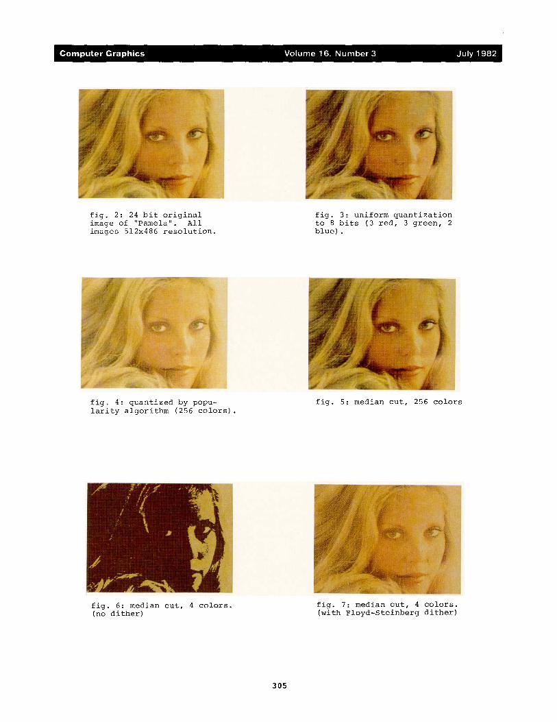
fig. 2: 24 bit original image of "Pamela". All images 512x486 resolution.

fig. 3: uniform quantization to 8 bits (3 red, 3 green, 2 blue).

fig. 4: quantized by popularity algorithm (256 colors).

fig. 5: median cut, 256 colors

fig. 6: median cut, 4 colors. (no dither)

fig. 7: median cut, 4 colors. (with Floyd-Steinberg dither)

305

fig. 8: 24 bit original image of "Marc".

fig. 9: uniform quantization to 8 bits (3 red, 3 green, 2 blue).

fig. i0: popularity algorithm, 256 colors.

fig. ll: median cut, 256 colors

fig. 12: median cut, with dither, 256 colors.

fig. 13: colormap for fig. 9 after 3 iterations of Lloyd's fixed point algorithm (256 colors).

306

fig. 14:24 bit original image of "Surface" (the surface of the RGB color cube unrolled).

fig. 15: popularity algorithm, 256 colors.

fig. 16: median cut, 256 colors.

fig. 17: median cut with dither, 256 colors.

fig. 18: exploded view of 16 tapered quantization cells in the RGB cube.

307

color image quantization -...

Documents