Collusion in Auctions with Constrained Bids:

Theory and Evidence from Public Procurement∗

Sylvain Chassang

Princeton University

Juan Ortner†

Boston University

August 28, 2015

preliminary and incomplete, do not quote, do not circulate

Abstract

We study the mechanics of cartel enforcement and its interaction with bidding con-straints in the context of repeated procurement auctions. Under collusion, biddingconstraints affect cartel behavior by limiting future pledgeable surplus. This yields atest of collusive behavior exploiting the counter-intuitive prediction that introducingminimum prices can lower the distribution of winning bids. The model’s predictionsare borne out in procurement data from Japan, where we find considerable evidencethat collusion is weakened by the introduction of minimum prices. An elementary the-ory of inference from observed bids lets us evaluate counterfactual policies.

Keywords: collusion, cartel enforcement, minimum prices, entry deterrence, pro-curement.

∗We are especially grateful to Rieko Ishii for pointing us towards appropriate data. The paper benefitedfrom comments by Chris Flynn, Hamid Sabourian, as well as feedback from seminar audiences at CollegioCarlo-Alberto, Cambridge University, and the University of Essex.

†Chassang: chassang@princeton.edu, Ortner: jortner@bu.edu.

1

1 Introduction

This paper studies the mechanics of cartel enforcement and its interaction with bidding

constraints in the context of repeated procurement auctions. We emphasize the role of self-

enforcement constraints in determining cartel behavior, and derive a test of collusion based

on the behavior of the right tail of winning bids following the introduction of minimum prices.

Minimum prices, which place a lower bound on the price at which procurement contracts

can be awarded, are frequently used in public procurement. We show that the introduction

of minimum prices makes cartel enforcement more difficult, yielding a first-order stochastic

dominance drop in the distribution of winning bids to the right of the minimum price. The

model’s predictions are borne out in procurement data from Japan, where the introduction

of minimum prices indeed shifts down the right tail of winning bids. In addition, the effect is

concentrated on bidders that are frequent participants, and auctions with a high reserve price,

providing strong empirical evidence that cartel self-enforcement constraints are binding, and

that minimum-prices undermine collusion. An elementary theory of inference from observed

bids lets us evaluate counterfactual policies, as well as perform overidentification tests of the

model.

We model firms repeatedly playing first-price procurement auctions. We assume that

production costs are i.i.d., commonly observed among cartel members, and that firms are

able to make transfers. Cartel behavior is limited by self-enforcement constraints: firms

must be willing to follow bidding recommendations, as well as make equilibrium transfers.

We provide an explicit characterization of optimal cartel behavior in this environment, and

contrast its predictions with those obtained from non-collusive models under a range of

information structures.

Our first set of results explores the effect of introducing minimum prices on the dis-

tribution of winning bids. In our repeated game environment, minimum prices weakens

cartel discipline by limiting the impact of price wars. As a result we show that introducing

2

minimum prices causes a first-order stochastic dominance drop in the distribution of win-

ning bids to the right of the minimum price: sustaining collusive bids above the minimum

price becomes more difficult. Minimum prices have the opposite impact in environments

without collusion: under complete information the right tail of winning bids is unchanged;

under asymmetric information, minimum prices generate a first order stochastic dominance

increase in the tail of wining bids.

Our second set of results provides a simple theory of inference from observed bids in the

presence of collusion. We show that collusion limits the scope for inference, but that it is

possible to partially identify the distribution of costs whenever the distribution of winning

bids has a non-trivial support. Indeed, in the case where the distribution of winning bids has

no atoms, the distribution of costs is identified up to a location parameter equal to the cartel’s

pledgeable surplus. Using our model to map distribution of costs to pledgeable surplus, we

obtain a fixed-point equation whose unique solution characterizes the distribution of costs.

We explore the empirical relevance of the mechanisms we study by using data from public

procurement auctions occuring in four Japanese cities between 2007 and 2015. The intro-

duction of minimum prices in one of our treatment cities in 2009 lets us use the difference-in-

difference framework of Athey and Imbens (2006) to recover the counterfactual distribution

of winning bids after the policy change. The data exhibits a large and significant drop in

the distribution of winning bids to the right of the minimum price, implying that: (i) en-

forcement constraints limit the scope of collusion; (ii) minimum prices successfully weaken

cartel discipline.

Richer data available from our treatment city lets us evaluate the channels through which

the distribution of winning bids is affected using a single difference approach. We show that

the effect of minimum prices is equally mediated by weakened entry deterrence, and weak-

ened enforcement among cartel members. Motivated by the fact that 25% of bidders make

up 80% of the (auction, bidder) pairs, we identify the top quartile of most active bidders as

cartel members. Consistent with our theory, the effect of minimum prices is entirely concen-

3

trated on cartel members. In addition, the effect of minimum prices is disporportionately

concentrated on auctions with a high reserve price, suggesting that enforcement constraints

are more binding for large auctions.

Our paper lies at the intersection of several strands in the literature on collusion in

auctions. The seminal work of Graham and Marshall (1987) and McAfee and McMillan

(1992) studies static collusion in environments where bidders are able to contract. A key

take-away from their analysis is that the optimal response from the auctioneer should involve

setting more constraining reserve prices – in a procurement setting this means reducing the

maximum price that the auctioneer is willing to pay. We argue, theoretically and empirically,

that when bidders cannot contract and must enforce collusion through repeated game play,

minimum prices constraining bids on the other side may also benefit the auctioneer by

weakening cartel enforcement.

An important observation of McAfee and McMillan (1992) is that in the absence of cash

transfers the cartel’s ability to collude is severly limited even when commitment is available.

A recent strand of work takes seriously the idea that in repeated games, continuation values

may successfully replace transfers. Aoyagi (2003) studies bid rotation schemes and allows

for communication. Skrzypacz and Hopenhayn (2004) (see also Blume and Heidhues, 2008)

study collusion in environments without communication and show that while cartel members

may still be able to collude, they will remain bounded away from efficient collusion. Athey

et al. (2004) study collusion in a model of repeated Bertrand competition and emphasize that

information revelation costs will push cartel members towards rigid pricing schemes. Our

model simplifies away many of the important strategic issues considered in this body of work

by assuming complete information among cartel members and transferability.1 As expected,

this allows us to provide a simple characterization of optimal collusion closely related to that

obtained in the relational contracting literature (Bull, 1987, Baker et al., 1994, 2002, Levin,

1Importantly, we allow for asymmetric information when we study the impact of minimum prices incompetitive environments.

4

2003). This lets us study the effect of price constraints on the distribution of winning bids,

as well as estimate the distribution of costs from observed winning bids.

Several recent papers study the impact of the allocation format on collusion. Fabra (2003)

compares the scope for tacit collusion in uniform and discriminatory auctions. Marshall and

Marx (2007) study the role of bidder registration and information revelation procedures in

facilitating collusion. Pavlov (2008) and Che and Kim (2009) consider settings in which

cartel members can commit to mechanisms and argue that appropriate auction design can

successfully limit the scope of collusion provided. Abdulkadiroglu and Chung (2003) make

a similar point when bidders are patient.

More closely related to our work, Lee and Sabourian (2011) as well as Mezzetti and Renou

(2012) study full implementation using dynamic mechanisms in a repeated environment.

They show that implementation in all equilibria can be achieved by restricting the set of

continuation values available to players to support repeated game strategies. The incomplete

contract literature (see for instance Bernheim and Whinston, 1998, Baker et al., 2002) has

suggested that the same mechanism used in the opposite direction provides foundations for

optimally incomplete contracts: in order to sustain efficient cooperation, it may be optimal

to keep contracts incomplete, thereby creating sufficient range in continuation play to enforce

efficient behavior. We provide empirical evidence that this mechanism plays a significant role

in practice, and can be meaningfully used to affect the level of collusion between parties.

On the empirical side, an important set of papers develops empirical methods to detect

collusion. Harrington (2008) provides a detailed survey of prominent empirical strategies and

their theoretical underpinnings. Porter and Zona (1993, 1999) contrast the behavior of sus-

pected cartel members with that of non-cartel members controlling for observables. Bajari

and Ye (2003) use excess correlation in bids as a marker of collusion. Porter (1983), along

with Ellison (1994) (see also Ishii, 2008) use patterns of price wars of the sort predicted by re-

peated game models of oligopoly behavior (Green and Porter, 1984, Rotemberg and Saloner,

1986) to identify collusion. In a multi-stage auction context, Kawai and Nakabayashi (2014)

5

argue that excess switching of second and third bidder across bidding rounds, compared to

first and second bidder, is a smoking gun for collusive aggreement.

An influential set of papers use structural methods to estimate deep payoff parameters.

This allows to estimate the costs of collusion as well evaluate potential counter-collusion

measures, such as raising reserve prices. Jofre-Bonet and Pesendorfer (2000, 2003), as well

as Bajari et al. (2007) consider models of repeated collusion in which equilibrium bidding

strategies have full support, and are Markovian with respect to observable states. In this

setting, they show that it is possible to estimate payoff-relevant parameters using only the

bidders’ incentive compatibility conditions without necessarily knowing which of many po-

tential equilibrium they may be playing. Asker (2010) studies the behavior of a known cartel

engaged in buying collectible stamps, for which extensive data is available.2 Using a pre-

cise theoretical model of the actual collusive scheme used by cartel members, he is able to

estimate their values for items being auctioned. As expected the cartel causes inefficiencies,

but interestingly the particular transfer scheme used by the cartel sometimes lead it to over-

bid. A consequence is that non-cartel members, rather than the auctioneer, suffer from the

cartel’s existence.

The paper is structured as follows. Section 2 sets up our benchmark model of cartel

behavior. Section 3 uses this model to derive a test of collusion as well as a simple theory of

identification. Section 4 briefly extends these results in a setting with entry. Section 5 takes

the model to data.

2 Self-Enforcing Cartels

Modeling strategy. McAfee and McMillan (1992)’s classic model of cartel behavior fo-

cuses on the constraints imposed by information revelation among cartel members. In-

stead we are interested in the enforcement of cartel recommendations through repeated play.

2See also Pesendorfer (2000) for a related exercise.

6

Viewed from the perspective of Myerson (1986), McAfee and McMillan (1992) focus on truth-

ful revelation, while we focus on obedience constraints. The implications of the two frictions

turn out to be different: McAfee and McMillan (1992) show that collusion makes lower

maximum prices desireable (in the context of procurement); we argue that higher minimum

prices may helpful in weakening cartels.

This different emphasis is reflected in our modeling choices. Our analysis has three main

goals:

(i) first, we want to provide clear intuition on how bidding constraints, here minimum

prices, affect cartel behavior and the distribution of bids;

(ii) second, we want to assess whether enforcement constraints are a significant de-

terminant of cartel behavior;

(iii) third, we want to provide a basic theory of inference from bids, permitting overi-

dentification tests of the model, as well as counterfactuals.

Given those goals, we try to be as general as possible when modeling the environments

we want to rule out, and go for simplicity and tractablity when modeling environments

of interest. Our preferred model of repeated game enforcement, assumes that costs are

common knowledge among cartel members and monetary transfers are feasible. In contrast,

our analysis of alternative competitive models studies a broader set of information structures.

2.1 The model

Players and payoffs. A buyer procures a single unit of a good at each period t ∈ N

through a first-price auction described below. A set N = {1, ..., n} of long-lived firms is

present in the market. In each period a subset Nt ⊂ N of firms is able to participate in the

auction. Participation is exogenous, i.i.d. over time, and cartel members are exchangeable.

In other terms, for all subsets J ⊂ N of cartel members, all permutations γ : N → N or

7

cartel member identities,

prob(Nt = J) = prob(Nt = σ(J)).

We think of this set of participating firms as those potentially able to produce in the

current period. Throughout the paper, participation is determined before production costs

become known.3 In period t, each participating firm i ∈ Nt can deliver the good at a cost

ci,t. Cost ci,t is drawn i.i.d. across participants and time periods from a c.d.f. F with support

[c, c] and density f .

Firms are able to send transfers to each other, regardless of whether or not they par-

ticipate in the auction. We denote by Ti,t the net transfer received or sent by firm i. Let

xi,t ∈ {0, 1} denote whether firm i wins the procurement contract in period t, let bi,t denote

her bid. We assume that firms have quasi-linear preferences, so that firm i’s overall stage

payoff is

πi,t = xi,t(bi,t − ci,t) + Ti,t.

Firms value future payoffs using a common discount factor δ < 1.

The stage game. The procurement contract is allocated according to a first price auction

with constrained bids. Specifically, each participant must submit a bid bi in the range [p, r]

where r is a maximum or reserve price, and p is a minimum price. Bids outside of this range

are discarded. The winner is the lowest bidder, and ties are broken with a uniform draw.

The winner then delivers the good at the price she bid.

All firms belong to the cartel, and, importantly, firms in the cartel observe one another’s

production costs. The assumption that costs are publicly observed by cartel members allows

for a tractable framework in which to study the effect that minimum prices have on bidding

behavior. Suppressing period index t, the timing of information and decisions within the

3We consider the endogenous participation of entrants in Section 4.

8

stage game is as follows:

1. The set of participating firms N is drawn and observed by all cartel members.

2. The production costs c = (ci)i∈N of participating firms are publicly observed by cartel

members.

3. Participating firms i ∈ N submit public bids b = (bi)i∈N , and the procurement contract

is publicly allocated, yielding public allocation x = (xi)i∈N ∈ {0, 1}N .

4. Firms can make transfers Ti.

Positive transfers are always accepted and only negative transfers will be subject to an

incentive compatibility condition. We require exact budget balance within each period at

the overall cartel level, i.e.∑

i∈N Ti = 0.

Our model is intended to capture common features of public procurement, especially of

procurement auctions for construction work. Governments running these auctions usually

need to procure on a regular basis. Moreover, they face a small and stable set of firms that can

potentially perform the work, a subset of which participates at each auction. Laws typically

require governments to make bids and outcomes public after each auction is completed. The

repeated nature of the interaction makes collusion a realistic concern. This motivates us

to study a model of cartel behavior in which collusion is enforced through repeated play.

To keep the model tractable and to focus on how enforcement constraints affect bidding

behavior, we assume that firms’ costs are public information and that transfers are feasible.4

Note that procurement auctions with minimum acceptable bids are frequently used in

practice. For instance, auctions with minimum bids are used for procurement of public

works in several countries in the European Union and by local governments in Japan. The

common rationale for introducing minimum bids in the auction is to limit defaults and costly

renegotiations from firms that win with very low bids.

4The assumption that firms can transfer money is not unrealistic. Indeed, many known cartels usedmonetary transfers; see for instance Asker (2010) and Harrington and Skrzypacz (2011). In practice thesetransfers can be made in ways that make it difficult for authorities to detect them, like sub-contractingbetween cartel members or, in the case of cartels for intermediate goods, intra-firm sales.

9

The repeated game. Interaction is repeated and firms can use the promise of continued

collusion to enforce obedient bidding and transfers. Formally, bids and transfers need to be

part of a subgame perfect equilibrium of the repeated games among firms.

The history among cartel members at the beginning of time t is

ht = {cs,bs,xs,Ts}t−1s=0.

Let Ht denote the set of period t public histories and H =⋃t≥0Ht denote the set of all

histories.

Our solution concept is subgame perfect equilibrium (SPE), with strategies

σi : ht 7→ (bi,t(ct), Ti,t(ct,bt,xt))

such that bids bi,t(ct) and transfers Ti,t(ct,bt,xt) can depend on all public data available at

the time of decision-making.

Definition 1 (collusive and non-collusive environments). We say that we are in a collusive

environment if firms play a Pareto efficient SPE.

We say that we are in a competitive environment if firms play a subgame perfect equilib-

rium of the stage game.

Clearly the hypothesis of collusive behavior is more restrictive than non-competitive

behavior would require. We address the concern by allowing for more general information

structures when evaluating alternative competitive models.

10

2.2 Optimal collusion

Denote by Σ the set of SPE in the repeated stage game. Let

V (σ, ht) = Eσ

∑s≥0

δs∑i∈N

xi,t+s(bi,t+s − ci,t+s)|ht

denote the total surplus generated under equilibrium σ conditional on history ht. We denote

by

V p ≡ supσ∈Σ

V (σ, h0)

the highest equilibrium surplus sustainable in equilibrium. We emphasize that this highest

equilibrium value depends on minimum price p.

Given a history ht and a strategy profile σ, we denote by β(ct|ht, σ) the bidding profile

induced by strategy profile σ at history ht as a function of realized costs ct.

Lemma 1 (stationarity). If an equilibrium σ attains V p, then σ delivers surplus V (σ, ht) =

V p after all on-path histories ht.

There exists a fixed bidding profile β∗ such that, in a Pareto efficient equilibria, firms bid

β(ct|ht, σ) = β∗(ct) after all on-path histories ht.

For any i ∈ N , let

Vi(σ, ht) = Eσ

[∑s≥0

δsxi,t+s(bi,t+s − ci,t+s)|ht

]

denote the expected discounted payoff that firm i gets in equilibrium σ conditional on history

ht. Let

V p ≡ infσ∈Σ

Vi(σ, h0)

denote the lowest possible equilibrium payoff for a firm.

Given a bidding profile β, let us denote by βW (c) and x(c) the induced winning bid and

11

allocation profile when realized costs are c. For each firm i, we define

ρi(βW ,x)(c) ≡ 1βW (c)>p +

1βW (c)=p∑j∈N,j 6=i 1xj(c)>0 + 1

.

When βW (c) > p, ρi(βW ,x)(c) corresponds to a deviator’s likelihood of winning the contract

by bidding below the equilibrium winning bid if βW (c) > p. Similarly, when βW (c) = p,

ρi(βW ,x)(c) corresponds to a deviator’s likelihood of winning the contract by bidding p.

Lemma 2 (enforceable bidding). A winning bid profile βW (c) and an allocation x(c) are

sustainable in SPE if and only if for all c,

∑i∈N

(ρi(βW ,x)(c)− xi(c))

[βW (c)− ci

]++ xi(c)

[βW (c)− ci

]− ≤ δ(V p − nV p). (1)

As in Levin (2003), a bidding profile can be implemented in a SPE if and only if the

sum of deviation temptations (both from bidders abstaining to bid above cost, and bidders

bidding below cost) is less than or equal the total pledgeable surplus δ(V p − nV p), i.e.

the difference between the highest possible continuation surplus, and the sum of minimal

surpluses guaranteed to a player in any equilibrium.

For each cost realization c, let x∗(c) denote the efficient allocation; i.e., it allocates the

procurement contract to the participating firm with the lowest cost (ties broken randomly).

We define

b∗p(c) ≡ sup

b ≤ r :∑i∈N

(1− x∗i (c)) [b− ci]+ ≤ δ(V p − nV p)

.

For values of c such that b∗p(c) > p, this value is the highest enforceable winning bid when

the cartel allocates the good efficiently.

Proposition 1. An optimal on-path bidding profile sets winning bid β∗p(c) = max{b∗p(c), p}

at every period. Moreover, the allocation is conditionally efficient: whenever β∗p(c) > p, the

contract is allocated to the bidder with the lowest procurement cost.

12

Our next result characterizes the firm’s behavior in a competitive environment. We use

the following notation: for any cost realization c, we let c(2) denote the second lowest cost.

Corollary 1 (behavior under competition). In a competitive environment, the cartel sets

winning bid β∗p(c) = max{p, c(2)}.

We now turn to study how minimum prices affect the set of payoffs that firms can sustain

in a SPE. We use the following assumption.

Assumption 1. c− c ≤ δ(V 0 − nV 0).

Assumption 1, which holds whenever the firms’ discount factor is large enough, guarantees

that the cartel has enough continuation surplus to provide incentives for participation.

Lemma 3 (worst case punishment). Under Assumption 1,

(i) V 0 = 0, and

(ii) there exists p > c such that, for all p ∈ (0, p), V p − nV p ≤ V 0 − nV 0. The inequalityis strict whenever p > c.

Lemma 3 (i) shows that, with no minimum price, the cartel can force a firm’s payoff

down to its min-max value of 0. Lemma 3 (ii) establishes that the net surplus V p − nV p

that the cartel can use to provide incentives decreases after introducing a minimum price.

Intuitively, a minimum price p > c increases the lowest equilibrium value V p and tightens

the enforcement constraint (1). This in turn reduces the bids that the cartel can sustain in

an optimal equilibrium, thereby reducing V p and leading to a further tightening of (1).

3 Empirical implications

3.1 The effect of minimum prices on the distribution of bids

We now turn to the empirical implications of our model. Our first result contrasts the effect

that a minimum price has on the winning bid distribution under competition and collusion.

13

Proposition 2 (the effect of minimum prices on bids). Fix p ∈ (0, p), and consider q > p.

(i) Under collusion, prob(β∗p > q|β∗p > p) ≤ prob(β∗0 > q|β∗0 > p), the inequality being strictfor some q > p whenever prob(β∗0 < r) > 0.

(i) Under competition, prob(β∗p > q|β∗p > p) = prob(β∗0 > q|β∗0 > p).

In words, under collusion introducing minimum prices induces a downward shift in the

tail of winning bids to the right of the minimum price. In contrast, under competition, the

introduction of minimum prices has no effects on the right tail of the winning bid distribution.

Section 5 uses this result to detect collusion in procurement data from Japan.

Predictions under competition and asymmetric information. Our model assumes

that procurement costs are publicly observable among cartel members. Under this assump-

tion, Proposition 2 (i) shows that, in a competitive environment, the introduction of a

minimum price leaves the right-tail of the distribution of winning bids unchanged. We now

show how this result extends if firms have private information about their procurement costs.

Suppose it is common knowledge that the procurement cost of each firm i ∈ N is drawn

i.i.d. from c.d.f. F with support [c, c] and density f . Each firm is privately informed about

its own procurement cost. Let bAI : [c, c]→ R+ be the bidding function in an equilibrium of

a first-price procurement auction with reserve price r and no minimum price.

Proposition 3. Under private information, a first-price auction with reserve price r and

minimum price p < r has a unique symmetric equilibrium with bidding function bAIp .

(i) If bAI(c) ≥ p, then bAIp (c) = bAI(c) for all c ∈ [c, c];

(ii) If bAI(c) < p, there exists a cutoff c ∈ (c, c) with bAI(c) > p such that

bAIp (c) =

{bAI(c) if c ≥ c,

p if c < c.

Proposition 3 characterizes the equilibrium of a first-price auction with minimum price p

when firms are publicly informed of their procurement costs. We note that, for p > bAI(c),

the bidding function bAIp has a discontinuity point at the threshold c.

14

For any cost vector c of participating firms, we let βAIp (c) ≡ mini bAIp (ci) denote the

winning bid.

Corollary 2. Fix p > 0. For all q > p, prob(βAIp > q | βAIp > p) ≥ prob(βAI0 > q | βAI0 > p).

3.2 Inferring the distribution of costs

Our next result shows that the c.d.f. of firms’ costs F is identified from bidding behavior in

auctions with two bidders. We start with a preliminary lemma.

Lemma 4. For any b ∈ [p, r),

F (b− δ(V p − nV p)) =

√prob(β∗p ≤ b|N = 2).

Lemma 4 can be used to identify the c.d.f. of firms’ cost from bidding data. For simplicity,

in the body of the text we focus on the case where the observed distribution of winning bids

does not have a mass point at the reserve price r, which is true in our data – Appendix

A.1 studies the more general. In addition, we maintain Assumption 1. By Lemma 4, for all

b ≤ r,

F (b− δV 0) =

√prob(β∗0 ≤ b|N = 2).

This equation shows that the distribution of costs is identified from bidding data up to

the location parameter δV 0. With knowledge of the firms’ discount factor, the location

parameter δV 0 can be identified as follows. For any value V ≥ 0, let FV denote the c.d.f. of

firms’ costs identified from bidding data when V 0 = V ; i.e., for any bid b < r, FV (b− δV ) =√prob(β∗0 ≤ b|N = 2). Let W (V ) denote the cartel’s expected discounted surplus from

playing the optimal collusive equilibrium when V 0 = V and the distribution of costs is FV .

Then, the total surplus V 0 is the solution to the fixed point equation W (V ) = V . The

following result summarizes this discussion.

15

Proposition 4 (inferring the distribution of values). Suppose that (i) Assumption 1 holds

and (ii) the distribution of winning bids does not have atoms. Then, the distribution of costs

is identified from the winning bid distribution in auctions with two bidders.

Finally, recall that the winning bid in a competitive environment is β∗0(c) = c(2). There-

fore, under competition, F (b) =

√prob(β∗0 ≤ b|N = 2) for all b < r; i.e., assuming competi-

tion when firms are colluding leads to an overestimation of procurement costs by a constant

δV 0.

4 Entry

We now extend the model in Section 2 to allow for entry. We assume that, in a addition

to participating cartel members N , at each period a short-lived firm may also bid in the

auction. To participate, the short-lived firm has to pay an entry cost kt. Entry cost kt is

drawn i.i.d. over time from distribution Fk with support [k, k]. We let Et ∈ {0, 1} denote

the entry decision of the short-lived firm in period t, with Et = 1 denoting entry.

Upon paying the entry cost, the short-lived firm learns its cost ce,t of delivering the good,

which is drawn i.i.d. from a c.d.f. Fe with support [c, c] and density fe. Finally, we assume

that the short-lived firm’s entry cost kt, her entry decision and her procurement cost ce,t are

publicly observed.

The timing of information and decisions within the stage game is as follows:

1. The short-lived firm’s entry cost k is drawn and publicly observed. The short-lived

firm makes her participation decision, which is observed by cartel members.

2. The set of participating cartel members is drawn and observed by cartel members and

short-lived firm.

3. The production costs c of participating firms are drawn and publicly observed by all

firms.

16

4. Participating firms submit public bids and the procurement contract is publicly allo-

cated.

5. Cartel members can make transfers Ti.

The public history at the beginning of time t is now ht = {ks, Es, cs,bs,xs,Ts}t−1s=0, and

is observed by both cartel members and entrants. Let Ht denote the set of period t public

histories and H =⋃t≥0Ht denote the set of all histories. Our solution concept is subgame

public equilibrium, with strategies

σi : ht 7→ (bi,t(kt, Et, ct), Ti,t(kt, Et, ct,bt,xt))

for cartel members and strategies

σe : ht 7→ (Et(kt), be,t(kt, ct))

for the short-lived firms.

The analysis of this model is essentially identical to that of the model of Section 2 except

that now the cartel must deter entry in addition to enforcing collusive bidding. For concision,

we focus on salient empirical features of this model. Appendix A provides details on optimal

cartel behavior.

Proposition 5 (the effect of minimum prices on bids). Fix p ∈ (0, p), and consider q > p.

(i) Under collusion, prob(β∗p > q|β∗p > p,E = 0) ≤ prob(β∗0 > q|β∗0 > p,E = 0). Theinequality is strict for some q > p whenever prob(β∗0 < r|E = 0) > 0.

(ii) Under competition, prob(β∗p > q|β∗p > p,E = 0) = prob(β∗0 > q|β∗0 > p,E = 0).

5 Empirical Analysis

The mechanism we delineate in Sections 2 and 4 is only effective if punishment is a binding

constraint on cartel behavior. There are also two channels by which price constraints may

17

affect cartel behavior: the first is greater entry of new firms, the second is worse enforcement

within the cartel. This begs the questions: are price constraints a relevant way to limit cartel

power? and, what is the relative importance of different channels in limiting cartel power?

We provide empirical answers to these questions using auction data from four Japanese

cities located in the Ibaraki prefecture: Hitachiomiya, Tsuchiura, Tsukuba and Ushiku.

The data covers public work projects auctioned off between May 2007 and March 2015,

corresponding to 4358 auctions, including 1565 for the treatment city alone.

Throughout the period, all cities use first-price auctions. On October 28th 2009, the city

of Tsuchiura implemented a policy change, moving from a zero minimum price to a strictly

positive minimum price ranging between 70% and 85% of the reserve price. The remaining

cities use first-price auctions with no minimum price throughout the period. This lets us

explore the effect of minimum prices on bidder behavior using a differences-in-differences

approach, using Tsuchiura as our treatment, and the three remaining cities as controls.

5.1 Some facts about the data

Sample selection. The sample of cities was selected as follows. In a study of paving

auctions, Ishii (2008) notes the use of minimum prices in Japanese procurement auctions.

The author was able to point us to data from Ibaraki Prefecture exhibiting required variation.

We then proceeded to search for all publicly available data from the 10 most populous cities

in the prefecture. We kept all cities that had public data available covering the relevant

policy change period. This left us with the four cities included in the study. The cities are

broadly comparable: their population ranges from 48K to 215K, with Tsuchiura at 143K.5

They are located within 75km of one another, and within 150km of Tokyo. None of our

results is sensitive to dropping one of the treatment cities.

5Tsuchiura also happens to be a sister city of Palo Alto, CA.

18

Policy change. The minimum prices used in our treatment city are chosen by a formal

rule and should not be interpreted as having any signalling content. Minimum prices range

between 70% to 85% of the reserve price, with the 25th, 50th and 75th quantiles respectively

at 80%, 82% and 84%. There is no evidence that the policy change was triggered by city

specific factors also affecting the distribution of bids. This is supported by the fact that all

of the control cities had switched to minimum prices by the end of 2014. Our understanding

is that minimum prices were introduced to remove bidders’ incentives to bid excessively low.

Descriptive statistics. Some facts about our sample of auctions are worth noting. The

first is that although all auctions include a reserve price, these reserve prices are not set to

extract greater surplus by the city along the lines of Myerson (1981) or Riley and Samuelson

(1981). Rather, consistent with recorded practice, reserve prices are engineering estimates

(Ohashi, 2009, Tanno and Hirai, 2012, Kawai and Nakabayashi, 2014), that provide an upper-

bound to the range of possible costs for the project. This is corroborated by the fact that

99.7% of auctions have a winner. This lets us treat reserve prices as an exogenous scaling

parameter and use it to normalize the distribution of bids to [0, 1]:

norm winning bid =bid

reserve price.6

The distribution of winning bids is closely concentrated near reserve prices. Indeed, the

mean cost savings from running an auction rather than using the reserve price as a take-it-

or-leave-it offer are equal to 4.9%. This could be because reserve prices are obtained through

very precise engineering estimates, but this provides justifiable concern that collusion may be

going on. It is also worth observing that the 10th quantile of the distribution of normalized

winning bids is equal to 83% of the reserve price. This means that minimum prices (set

6Table 7 suggests that the distribution of reserve prices is unaffected by treatment.

19

within 70% and 85% of reserve prices) are in the low quantile of the distribution of winning

bids (the median minimum price is in the first decile of the distribution of winning bids).

Propositions 2 and 5 suggest that absent collusive dynamics, this should lead to a weakly

positive first-order stochastic dominance increase in the right tail of winning bids.

5.2 The impact of minimum prices on the distribution of winning

bids

Figure 1 plots distributions of winning bids in treatment and control cities before and after

treatment. The data shows a clear pattern making it highly suitable for a differences in

differences approach. The distribution of bids in the control cities is unchanged, while the

distribution of the treatment city to the right of reserve prices experiences a significant

first-order stochastic dominance drop.

This observation vindicates the mechanism that we analyze in Sections 2, 3 and 4. There

is collusion in the data, and the sustainability of collusion is limited by price constraints.

This visual assessment can be made formal using the differences-in-differences framework of

Athey and Imbens (2006).

Differences-in-differences. Following Athey and Imbens (2006) we use the differences

in differences setup to compute counterfactual estimates of the distribution of winning bids

in our treatment city, absent minimum prices. We report here results using Hitachiomiya

and Ushiku as a control: data from Hitachiomiya, Ushiku and Tsuchuria are all available by

May 2008, whereas data from Tsukuba only become available after May 2009. We provide

results including Tsukuba in Appendix A: the main findings are unchanged.

Propositions 2 and 5 make clear predictions: if there is no-collusion the introduction of

a minimum price should not change the right tail of wining bids; if there is collusion, we

anticipate a drop in the right tail of winning bids. The actual and counterfactual quantiles

20

0.5 0.6 0.7 0.8 0.9 1.0normalized winning bids

0.0

0.2

0.4

0.6

0.8

1.0

shar

e of

auc

tions

hitachiomiya, cdf of normalized winning bids

beforeafter

(a) control: Hitachiomiya

0.4 0.5 0.6 0.7 0.8 0.9 1.0normalized winning bids

0.0

0.2

0.4

0.6

0.8

1.0

shar

e of

auc

tions

tsukuba, cdf of normalized winning bids

beforeafter

(b) control: Tsukuba

0.4 0.5 0.6 0.7 0.8 0.9 1.0normalized winning bids

0.0

0.2

0.4

0.6

0.8

1.0

shar

e of

auc

tions

ushiku, cdf of normalized winning bids

beforeafter

(c) control: Ushiku

0.3 0.4 0.5 0.6 0.7 0.8 0.9 1.0normalized winning bids

0.0

0.2

0.4

0.6

0.8

1.0

shar

e of

auc

tions

tsuchiura, cdf of normalized winning bids

beforeafter

(d) treatment: Tsuchiura

Figure 1: distribution of winning bids, before and after treatment: 2007-2009, 2009-2011.

of normalized winning bids, conditional on prices being above 80% of the reserve price are

given in Table 1 and Figure 2.7

The data is unequivocal. There is collusion. The cartel is constrained by enforcement

constraints. These enforcement constraints are worsened by the introduction of minimum

prices.

7The results are unchanged if we consider the distribution of normalized winning bids conditional onprices being above .75, .82, or .85 of the reserve price, or if we use raw winning bids. See Appendix A fordetails.

21

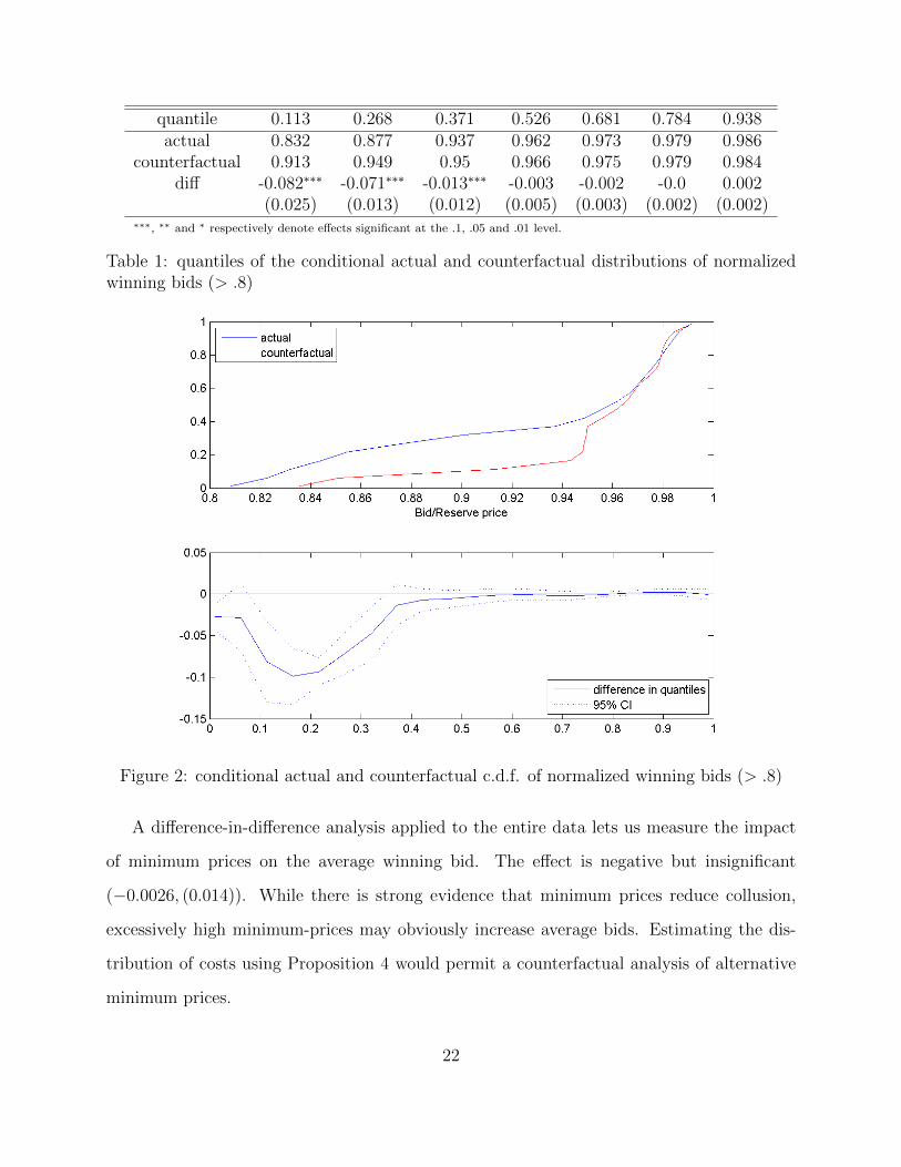
quantile 0.113 0.268 0.371 0.526 0.681 0.784 0.938actual 0.832 0.877 0.937 0.962 0.973 0.979 0.986

counterfactual 0.913 0.949 0.95 0.966 0.975 0.979 0.984diff -0.082∗∗∗ -0.071∗∗∗ -0.013∗∗∗ -0.003 -0.002 -0.0 0.002

(0.025) (0.013) (0.012) (0.005) (0.003) (0.002) (0.002)∗∗∗, ∗∗ and ∗ respectively denote effects significant at the .1, .05 and .01 level.

Table 1: quantiles of the conditional actual and counterfactual distributions of normalizedwinning bids (> .8)

Figure 2: conditional actual and counterfactual c.d.f. of normalized winning bids (> .8)

A difference-in-difference analysis applied to the entire data lets us measure the impact

of minimum prices on the average winning bid. The effect is negative but insignificant

(−0.0026, (0.014)). While there is strong evidence that minimum prices reduce collusion,

excessively high minimum-prices may obviously increase average bids. Estimating the dis-

tribution of costs using Proposition 4 would permit a counterfactual analysis of alternative

minimum prices.

22

Single city regression. Our analysis going forward focuses on better understanding the

channels by which price constraints affect the distribution of winning bids. For this pur-

pose, we must rely on data from our treatment city alone. This is due to data restrictions:

public data available from our treatment city provides detailed information about individual

auctions, including the names of bidders and their bids.

We use a regression discontinuity design and begin by replicating the results from our

differences-in-differences framework. We define variables

window = 1date∈{October 28th 2009±12 months},

policy change = window × 1date≥October 28th 2009

and perform both OLS and quantile regressions on the linear model

norm winning bid ∼ β0 + β1window + β2policy change+ βcontrols (2)

where controls (used throughout the analysis) include Japanese logGDP as well as the

current year.

norm winning bid mean 25th quantile 50th quantilewindow 0.001 -0.002 0.003

(0.007) (0.01) (0.004)policy change -0.021∗∗∗ -0.077∗∗∗ -0.011∗∗∗

(0.006) (0.008) (0.003)lnGDP 0.434∗∗∗ 0.457∗∗∗ 0.107∗∗∗

(0.068) (0.101) (0.04)year 0.005∗∗∗ 0.003∗ 0.003∗∗∗

(0.001) (0.002) (0.001)

Table 2: the effect of minimum prices on winning bids

While the results are not precisely identical, these magnitudes match those of our differences-

in-differerences design, which gives us some confidence that we control for enough time-

23

varying covariates to justify a single-city analysis. Note that the drop in normalized winning

bids obtained from this regression, −2.1%, is large given that the mean cost saving from

running an auction rather than using reserve-prices as take-it-or-leave-it offers is roughly

5%.8

5.3 The Impact of minimum prices on entry and cartel behavior

We now wish to better understand the channels through which minimum prices affect the

distribution of winning bids. Specifically, we are interested in understanding how the effect of

minimum prices breaks down along greater entry, and worse collusion among cartel members,

keeping entry constant.

Consistent with the theory, we define cartel members and entrants according to the

frequency with which they participate in auctions. Our treatment city exhibits considerable

heterogeneity in the degree of bidder activity over the seven years spanned by our data. The

median number of auctions a bidder participates in is 4, whereas the average is at 22. As a

result, the 25% most active bidders make up 80% of the auction×bidder data. Accordingly,

we define as cartel members this 25th quantile of the most active bidders (58 out of 234 total

number of bidders). We define entrants as non-cartel-members.

Greater entry vs. worse collusion. We assess the relative importance of greater entry

and worst enforcement by first assessing the impact of minimum prices on entry, and second

assessing the impact of minimum prices on winning bids, controlling for entry. For greater

robustness, we report regressions using both the number of entrants, and the total number

of bidders to measure broader participation by cartel members.

As expected, minimum prices increase both entry and participation. Table 3 reports the

8This reduction in normalized winning bids underestimates aggregate cost-savings: we show below thatthe bulk of the effect of minimum prices is on high-cost projects.

24

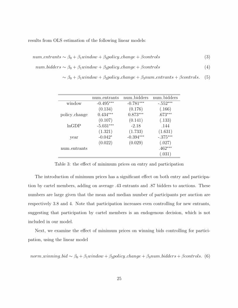
results from OLS estimation of the following linear models:

num entrants ∼ β0 + β1window + β2policy change+ βcontrols (3)

num bidders ∼ β0 + β1window + β2policy change+ βcontrols (4)

∼ β0 + β1window + β2policy change+ β3num entrants+ βcontrols. (5)

num entrants num bidders num bidderswindow -0.495∗∗∗ -0.781∗∗∗ -.552∗∗∗

(0.134) (0.176) (.166)policy change 0.434∗∗∗ 0.873∗∗∗ .673∗∗∗

(0.107) (0.141) (.133)lnGDP -5.031∗∗∗ -2.18 .144

(1.321) (1.733) (1.631)year -0.042∗ -0.394∗∗∗ -.375∗∗∗

(0.022) (0.029) (.027)num entrants .462∗∗∗

(.031)

Table 3: the effect of minimum prices on entry and participation

The introduction of minimum prices has a significant effect on both entry and participa-

tion by cartel members, adding on average .43 entrants and .87 bidders to auctions. These

numbers are large given that the mean and median number of participants per auction are

respectively 3.8 and 4. Note that participation increases even controlling for new entrants,

suggesting that participation by cartel members is an endogenous decision, which is not

included in our model.

Next, we examine the effect of minimum prices on winning bids controlling for partici-

pation, using the linear model

norm winning bid ∼ β0 + β1window+ β2policy change+ β3num bidders+ βcontrols. (6)

25

norm winning bid mean 25th quantile 50th quantilewindow -0.008 -0.009 -0.004

(0.007) (0.011) (0.004)policy change -0.01∗∗ -0.055∗∗∗ -0.01∗∗∗

(0.005) (0.009) (0.003)num bidders -0.012∗∗∗ -0.011∗∗∗ -0.01∗∗∗

(0.001) (0.002) (0.001)lnGDP 0.408∗∗∗ 0.392∗∗∗ 0.096∗∗

(0.065) (0.105) (0.038)year 0.0 -0.002 -0.001

(0.001) (0.002) (0.001)

Table 4: the effect of minimum prices on winning bids, controlling for participation

whose estimates are reported in Table 4. Regression (6) assigns similar shares of the drop

in normalized winning bids (−2.1%, Table 2) to the greater-entry channel (−1.2% × .87 =

1.04%) and the worst-collusion channel (−1%). This suggests that the total effect of mini-

mum prices on winning bids is mediated in roughly equal shares through greater entry, and

worst enforcement among cartel members.

Who does the policy change affect? We obtain further vindication of the mechanism

analyzed in Sections 2, 3 and 4 by distinguishing the effect of minimum prices on cartel

members and entrants. Our theory predicts that the price paid by winning cartel members

should go down, but not the price paid by winning entrants. We assess this hypothesis by

estimating the linear model

norm winning bid ∼ β0 + β1window + β2cartel winner + β3policy change (7)

+ β4cartel winner × policy change+ βcontrols

whose estimates are reported in Table 5. The findings are entirely consistent with the theory.

Absent minimum prices, cartel winners obtain contracts at higher prices. The introduction

of minimum prices reduces winning bids only when a cartel member is the winner.

26

normalized winning bidcartel winner 0.027∗∗∗ 0.028∗∗∗

(0.005) (0.005)cartel winner × policy change -0.027∗∗∗ -0.022∗∗

(0.009) (0.009)window 0.0 -0.009

(0.007) (0.007)policy change 0.002 0.009

(0.009) (0.009)lngdp 0.428∗∗∗ 0.399∗∗∗

(0.068) (0.065)year 0.005∗∗∗ 0.0

(0.001) (0.001)num bidders -0.012∗∗∗

(0.001)

Table 5: the effect of minimum prices on cartel members and entrants

Auction size. The mechanism we develop in Sections 2, 3 and 4 argues that minimum

prices affect the sustainability of collusion by reducing enforcement capabilities, or in other

terms by reducing the pledgeable surplus across cartel members. This mechanism should be

stronger when obedience constraint (1) binds. If auction size varies over time, the deviation

temptation will vary over time whereas continuation values will remain stable. Hence, if our

mechanism is the correct one, we should expect minimum prices to have a larger effect on

larger auctions.

The scale of projects, measured by their reserve price, exhibits sufficient heterogenity to

implement this test: the 25th, 50th and 75th quantiles being respectively at ¥5M, ¥13M, and

¥29M. We define an auction as large whenever its reserve price is above the 75th quantile of

reserve prices and estimate relationships of the form

norm winning bid ∼β0 + β2cartel winner + β3cartel winner × policy change (8)

+ β4window + β5policy change+ βcontrols

27

norm winning bid if large if not largecartel winner 0.026∗∗∗ 0.025∗∗∗ 0.027∗∗∗ 0.026∗∗∗

(0.009) (0.008) (0.006) (0.006)cartel winner × policy change -0.059∗∗∗ -0.056∗∗∗ -0.019∗ -0.013

(0.018) (0.016) (0.011) (0.01)window -0.011 -0.012 0.004 -0.007

(0.012) (0.011) (0.008) (0.008)policy change 0.025 0.025 -0.003 0.006

(0.017) (0.016) (0.01) (0.01)lngdp 0.177 0.396∗∗∗ 0.526∗∗∗ 0.452∗∗∗

(0.116) (0.107) (0.082) (0.079)year 0.006∗∗∗ -0.003 0.004∗∗∗ 0.0

(0.002) (0.002) (0.001) (0.001)num bidders -0.016∗∗∗ -0.012∗∗∗

(0.002) (0.001)

Table 6: the effect of minimum prices for large and small auctions

conditional on auction size.

Table 6 shows that the effect of minimum prices is indeed concentrated on cartel mem-

bers participating in large auctions. The effect of the policy on cartel members is either

insignificant or much smaller for small auctions, the difference in coefficients (−5.9% for

large auctions, versus −1.9% for smaller auctions) being significant at the 5% level.

6 Discussion

Summary. We provide a tractable framework to analyze the effect of price constraints on

repeated collusion. Our model delivers a simple intuition: price constraints limit the range

of continuation equilibria, making cartel enforcement and entry deterrence more difficult.

Our model also yields a simple empirical prediction: under collusion, the introduction of

minimum prices should yield a first order stochastic dominance drop in the distribution of

winning bids. In addition, we can use our characterization of optimal bidding to infer costs

from the distribution of bids.

Our test finds strong evidence of collusion in procurement data from Japan, validating the

28

hypothesis that enforcement constraints are binding, and that price constraints can weaken

enforcement.

Limits. Some limits of our framework are worth highlighting. One is that we do not model

participation by cartel members. We simply treat it as exogenous. However it may well be

optimal to limit the set of auctions that firms can participate in. We also elude collusion

under asymmetric information, and heterogeneity among bidders. While this limits the scope

of our inference results, this does not affect the meaningfulness of our test of collusion. In

competitive environments, whether or not there is asymmetric information, the introduction

of minimum prices leads to a first-order stochastic dominance increase in the right tail of the

distribution of bids.

Design. Using minimum prices to reduce collusion requires thoughtfully calibrating the

level of the minimum price to ensure that it is not excessively high. However, minimum

prices below the observed distribution of winning bids can only help. One subtlety worth

emphasizing is that the minimum prices we explore are fixed, and not indexed on bids. In

some settings (e.g. Italy) minimum bids are set as an increasing function of other bidders’

bids (e.g. a quantile of submitted bids, Conley and Decarolis (2011), Decarolis (2013)).

We expect such minimum price schemes to be less effective than fixed minimum prices in

deterring collusion: by coordinating low bids, cartel bidders can bring minimum prices down

off equilibrium.

29

Appendix

A Additional Results

A.1 Inferring the distribution of costs – general case

This appendix extends the results in Section 3.2 to the case in which the observed distribution

of winning bids has a mass point at the reserve price. We show that in this case we can

obtain bounds on V 0. For simplicity, we maintain Assumption 1. We also assume that the

support [c, c] of the cost distribution F is such that c ≤ r, which is true in our data.9

By Lemma 4, for all c < r − δV 0

F (c) =

√prob(β∗0 ≤ c+ δV 0|N = 2). (9)

Since the reserve price is an upper bound to procurement costs,

probF (c ∈ [r − δV 0, r]) = 1−√

prob(β∗0 < r|N = 2). (10)

For any V ≥ 0, let FV be the set of all c.d.f. that are consistent with (9) and (10) when

V 0 = V . For any F ∈ FV , let W (F, V ) be the cartel’s expected discounted surplus from

playing the optimal collusive equilibrium when V = V and the distribution of cost is F .

Let Wmax(V ) = supF∈FVW (F, V ) and Wmin(V ) = infF∈FV

W (F, V ). Finally, let V max and

V min be, respectively, the solutions to the fixed point equations V max = Wmax(V max) and

V min = Wmin(V min), so that V max > V min. Then, the cartel’s total surplus V 0 is be bounded

by V min and V max; i.e., V 0 ∈ [V min, V max].

9Indeed, 99.7% of all the auctions in our dataset have a winner.

30

A.2 Collusion under threat of entry

This appendix analyzes the model with entry in Section 4. We let Ne denote the set of all

participants in the auction; i.e., Ne = N when E = 0, and Ne = N ∪ {e} when E = 1.

Given a history ht and an equilibrium σ, we let β(k, c|ht, σ) be the bidding profile of cartel

members and short-lived firm induced by σ at history ht as a function of realized entry cost

k and procurement costs c = (ci)i∈Ne.10 Our first result generalizes Lemma 1 to the current

setting.

Lemma A.1 (stationarity – entry). If an equilibrium σ attains V p, then σ delivers surplus

V (σ, ht) = V p after all on-path histories ht.

There exists a fixed bidding profile β∗ such that, in a Pareto efficient equilibrium, firms

bid β(k, ct|ht, σ) = β∗(k, ct) after all on-path histories ht.

Given a bidding profile β, we let βW (c) be the winning bid and x(c) = (xi(c))i∈Nebe the

induced allocation when realized costs are c = (ci)i∈Ne. As in Section 2, for all i ∈ Ne we let

ρi(βW ,x)(c) ≡ 1βW (c)>p +

1βW (c)=p∑j∈Ne,j 6=i 1xj(c)>p + 1

.

Lemma A.2 (enforceable bidding – entry). A winning bid profile βW (c) and an allocation

x(c) are sustainable in SPE if and only if, for E ∈ {0, 1} and for all c,

∑i∈N

{(ρi(βW ,x)(c)− xi(c))[βW (c)− ci]+ + xi(c)[βW (c)− ci]−} ≤ δ(V p − nV p). (11)

E × {(ρe(βW ,x)(c)− xe(c))[βW (c)− ce]+ + xe(c)[βW (c)− ce]−} ≤ 0. (12)

For any bidding profile β that is sustainable in a SPE, let πe(β) denote the expected

payoff that a short-lived bidder gets when it enters the auction and participating firms bid

10Since the vector of costs c includes the cost of the short-lived firm in case of entry, the cartel’s biddingprofile can be different depending on whether the short-lived firm enters the auction or not.

31

according to β. Let πep ≡ inf{πe(β) : β satisfies equations (11) and (12)}. Note that the

cartel can guarantee that all firms with entry cost larger than πep don’t participate in the

auction by playing a sustainable bidding profile that attains πep when the short-lived firm’s

entry cost is larger than πep.

Our next result shows that minimum prices reduce the cartel’s ability to deter entry.

Lemma A.3 (entry deterrence). For all p > 0, πep ≥ πe0 = 0, with strict inequality if p > c.

Recall that

b∗p(c) = sup

b ≤ r :∑i∈N

(1− x∗i (c)) [b− ci]+ ≤ δ(V p − nV p)

.

We use the following notation: for any cost vector c, we let c(1) = mini∈N ci be the lowest

cost among participating cartel members.

Proposition A.1. In an optimal equilibrium, the on-path bidding profile is such that:

(i) if E = 0, the cartel sets winning bid β∗p(c) = max{b∗p(c), p};

(ii) if E = 1, a cartel member wins the auction only if c(1) ≤ max{ce, p}; the winning

bid is β∗p(c) = max{p,min{ce, b∗p(c)}} when a cartel wins the auction, and is β∗p(c) =

max{c(1), p} when the entrant wins the auction.

A short-lived firm enters the auction if and only if k ≤ πep.

Proposition A.1 characterizes bidding behavior under an optimal equilibrium. In periods

in which the short-lived firm does not participate, the cartel’s bidding behavior is the same

as in Section 2. Entry by a short-lived firm reduces the cartels profits in two ways: (i) the

cartel losses the auction whenever the entrant’s procurement cost is low enough, and (ii)

entry leads to weakly lower winning bids when the cartel wins the auction.

For any cost vector c = (ci)i∈Ne, let c(2) be the second lowest cost among participating

firms.

32

Corollary A.1. In a competitive environment, for any c the winning bid is β∗p(c) = max{c(2), p}.

Our last result in this section extends Lemma 3 to the current setting.

Lemma A.4 (worse case punishment – entry). Under Assumption 1,

(i) V 0 = 0;

(ii) there exists p > c such that, for all p ∈ (0, p), V p − nV p ≤ V 0 − nV 0. The inequalityis strict whenever p > c.

B Robustness of Empirical Findings

We test whether reserve prices are affected by the policy change by running the regression

log reserve price ∼ β0 + β1window + β3policy change+ βcontrols.

The results, summarized in Table 7, suggest that this is by and large not the case, except

perhaps at the higher quantiles. Furthermore the effect, if any, seems to be a reduction

in reserve prices, which would tend to strengthen our results: minimum prices can bring

normalized winning bids down even starting from lower reserve prices.

log reserve price mean 25th quantile 50th quantilewindow -0.025 -0.015 0.181

(0.116) (0.169) (0.159)policy change -0.132 -0.073 -0.374∗∗∗

(0.092) (0.135) (0.127)lnGDP -1.778 0.403 0.707

(1.136) (1.665) (1.559)year 0.086∗∗∗ 0.048∗ 0.088∗∗∗

(0.019) (0.028) (0.026)

Table 7: The impact of treatment on reserve-prices

33

C Proofs

C.1 Proofs for Section 2

This appendix contains the proofs of Section 2. We assume for now that the lowest SPE

payoff V p can be attained. Lemma 3 provides sufficient conditions under which this is true.

We start with a few preliminary observations. Fix a SPE σ and a history ht. Let β(c) and

T (c,b,x) be the bidding and transfer profile that firms play in this equilibrium after history

ht, and let x(c) be the allocation induced by bidding profile β(c). Let ht+1 = htt (c,b,x,T)

be the concatenated history composed of ht followed by (c,b,x,T), and let {V (ht+1)}i∈N

be the vector of continuation payoffs after history ht+1. For each c, let βW (c) and x(c) be,

respectively, the winning bid and the allocation. Recall that

ρi(βW ,x)(c) = 1βW (c)>p +

1βW (c)=p∑j∈N,j 6=i 1xj(c)>0 + 1

.

To economize on notation, we let ht+1(c) = ht t (c, β(c),x(c),T(c, β(c),x(c))) denote the

on-path history that follows ht when current costs are c. Note that the following inequalities

must hold:

(i) for all i ∈ N such that ci ≤ βW (c),

xi(c)(βW (c)− ci) + Ti(c, β(c),x(c)) + δVi(ht+1(c)) ≥ ρi(βW ,x)(c)(βW (c)− ci) + δV p.

(13)

(ii) for all i ∈ N such that ci > βW (c),

xi(c)(βW (c)− ci) + Ti(c, β(c),x(c)) + δVi(ht+1(c)) ≥ δV p. (14)

(iii) for all i ∈ N ,

Ti(c, β(c),x(c)) + δVi(ht+1(c)) ≥ δV p. (15)

The inequality in (13) must hold since a firm with cost below βW (c) can obtain a payoff at

least as large as the right-hand side by undercutting the winning bid when βW (c) > p, or,

34

by bidding p when βW (c) = p. Similarly, the inequality in (14) must hold since firms with

cost larger than βW (c) can obtain a payoff at least as large as the right-hand side by bidding

more than βW (c). Finally, the inequality in (15) must hold since otherwise firm i would not

be willing to make the required transfer.

Conversely, suppose there exists a winning bid profile βW (c), an allocation x(c), a transfer

profile T and equilibrium continuation payoffs {Vi(ht+1(c)}i∈N that satisfy inequalities (13)-

(15). Then, (βW ,x,T) can be supported in a SPE as follows. For all c, firms i ∈ N with

xi(c) > 0 bid βW (c), and firms i ∈ N with xi(c) = 0 bid βi(c) > βW (c). If no firm deviates

at the bidding stage, firms make transfers Ti(c, β(c),x(c)). If no firm deviates at the transfer

stage, in the next period firms play an SPE that gives payoff vector {V (ht+1(c))}i∈N . If firm

i deviates at the bidding stage, there are no transfers and the cartel reverts to an equilibrium

that gives firm i a payoff of V p; if firm i deviates at the transfer stage, the cartel reverts to an

equilibrium that gives firm i a payoff of V p (deviations by more than one firm go unpunished).

Since (13) holds, under this strategy profile no firm has an incentive to undercut the winning

bid βW (c). Since (14) holds, no firm with ci > βW (c) and xi(c) > 0 has an incentive to bid

above βW (c) and lose.11 Finally, since (15) holds, all firms have an incentive to make their

required transfers.

Proof of Lemma 1. Let σ be a SPE that attains V p. Towards a contradiction, sup-

pose there exists an on-path history ht = ht−1 t (c, β(c),x(c),T(c, β(c),x(c))) such that∑i Vi(σ, ht) = V (σ, ht) < V p. Let {Vi}i∈N be an equilibrium payoff vector with

∑i Vi = V p.

Consider changing the continuation equilibrium at history ht by an equilibrium that

delivers payoff vector {Vi}i∈N , and changing the transfers after history ht−1 t (c, β(c),x(c))

as follows. First, for each i ∈ N , let Ti be such that Ti + δVi = Ti(c, β(c),x(c)) + δVi(σ, ht).

Note that ∑i

Ti =∑i

{Ti(c, β(c),x(c)) + δ(Vi(σ, ht)− Vi)} < 0,

11Upward deviations by a firm i with ci < βW (c) who bids βW (c) and wins with probability 1 can bedeterred by having the lowest cost firm who losses the auction randomize over an interval [βW (c), βW (c)+ε].

35

where we used∑

i Vi = V p >∑

i Vi(σ, ht) and∑

i Ti(c, β(c),x(c)) = 0. For each i ∈ N , let

Ti = Ti + εn, where ε > 0 is such that

∑i Ti =

∑i Ti + ε = 0. Replacing Ti(c, β(c),x(c))

by Ti relaxes constraints (13)-(15) and increases the total expected discounted surplus that

the equilibrium generates. Therefore, if σ attains V p, it must be that V (σ, ht) = V p for all

on-path histories ht.

We now prove the second statement in the Lemma. Fix an optimal equilibrium σ, and

let {Vi}i∈N be the equilibrium payoff vector that this equilibrium delivers, with∑

i Vi = V p.

Let β be the bidding profile that firms use in the first period under σ, and let x(c) denote

the allocation induced by bidding profile β. It follows that

V p = E

∑i∈N

xi(c)(βi(c)− ci)

+ δV p ⇐⇒ V p =1

1− δE

∑i∈N

xi(c)(βi(c)− x(c))

.We show that there exists an optimal equilibrium in which firms use bidding profile β after

all on-path histories. For any (c,b,x), let Ti(c,b,x) denote the transfer that firm i makes at

the end of the first period under equilibrium σ when first period costs, bids and allocation are

given by c, b and x. Let Vi(h1(c)) denote firm i’s continuation payoff under equilibrium σ

after first period history h1(c) = (c, β(c),x(c)). By our arguments above,∑

i Vi(h1(c)) = V p

for all c. Since σ is an equilibrium, it must be that β(c), x(c) and Vi(h1(c)) satisfy (13)-(15).

Consider the following strategy profile. Along the equilibrium path, at each period t

firms bid according to β. For any (c, β(c),x(c)), firm i makes transfer Ti(c, β(c),x(c)) such

that Ti(c, β(c),x(c)) + δVi = Ti(c, β(c),x(c)) + δVi(h1(c)). Note that

∑i

Ti(c, β(c),x(c)) =∑i

{Ti(c, β(c),x(c)) + δ(Vi(h1(c))− Vi)} = 0,

where we used∑

i Ti(c, β(c),x(c)) = 0 and∑

i Vi(h1(c)) = V p =∑

i Vi. If firm i deviates

at the bidding stage or transfer stage, then firms revert to an equilibrium that gives firm i

a payoff of V p. Clearly, this strategy profile delivers total payoff V p. Moreover, firms have

36

weakly stronger incentives to bid according to β and make their required transfers than un-

der the original equilibrium σ. Hence, no firm has an incentive to deviate and this strategy

profile can be supported as an equilibrium. �

Proof of Lemma 2. Suppose there exists a SPE σ and a history ht in which firms

bid according to a bidding profile β that induces winning bid βW (c) and allocation x(c).

Let Ti(c, β(c),x(c)) be firm i’s transfers at history ht when costs are c and all firms play

according to the SPE σ. Let ht+1(c) = ht t (c, β(c),x(c),T(c, β(c),x(c))) be the on-path

history that follows ht when costs are c, and let Vi(ht+1(c)) be firm i’s equilibrium payoff at

history ht+1(c). Since the equilibrium must satisfy (13)-(15), it follows that for all c,

∑i∈N

{(ρi(β

W ,x)(c)− xi(c))[βW (c)− ci

]++ xi(c)

[βW (c)− ci

]−}≤∑i∈N

Ti(c, β(c),x(c)) + δ∑i∈N

(Vi(ht+1(c))− V p) ≤ δ(V p − nV p),

where we used∑

i Ti(c, β(c),x(c)) = 0 and∑

i Vi(ht+1(c)) ≤ V p.

Next, consider a winning bid profile βW (c) and an allocation x(c) that satisfies (1) for

all c. We now construct a SPE that supports βW and x in the first period. Let {Vi}i∈N be

an equilibrium payoff vector with∑

i Vi = V p. For each i ∈ N and each c, we construct

transfers Ti(c) as follows:

Ti(c) =

−δ(Vi − V p) + (ρi(β

W ,x)(c)− xi(c))(βW (c)− ci) + ε(c) if i ∈ N , ci ≤ βW (c),

−δ(Vi − V p) + xi(c)(βW (c)− ci) + ε(c) if i ∈ N , ci > βW (c),

−δ(Vi − V p) + ε(c) if i /∈ N ,

37

where ε(c) ≥ 0 is a constant to be determined below. Note that, for all c,

∑i∈N

Ti(c)− nε(c)

=− δ(V p − nV p) +∑i∈N

{(ρi(β

W ,x)(c)− xi(c))[βW (c)− ci

]++ xi(c)

[βW (c)− ci

]−} ≤ 0,

where the inequality follows since βW and x satisfy (1). We set ε(c) ≥ 0 such that transfers

are budget balance; i.e., such that∑

i∈N Ti(c) = 0.

The SPE we construct is as follows. At t = 0, for each c, firms with xi(c) > 0 bid βW (c)

and firms with xi(c) = 0 bid βi > βW (c). If no firm deviates at the bidding stage, firms

exchange transfers Ti(c). If no firm deviates at the transfer stage, from t = 1 onwards they

play a SPE that supports payoff vector {Vi}. If firm i ∈ N deviates either at the bidding

stage or at the transfer stage, from t = 1 onwards firms play a SPE that gives firm i a

payoff V p (if more than one firm deviates, then firms punish the lowest indexed firm that

deviated). One can check that this strategy profile satisfies (13)-(15), and so βW and x are

implementable. �

Proof of Proposition 1. By Lemma 1, if there exists an optimal equilibrium, then there

exists an optimal equilibrium in which firms use the same bidding profile β at every on-path

history. For each cost vector c, let βW (c) and x(c) denote the winning bid and the allocation

induced by this bidding profile under cost vector c.

We first show that βW (c) = b∗p(c) for all c such that b∗p(c) > p. Towards a contradiction,

suppose there exists c with βW (c) 6= b∗p(c) > p. Since x∗(c) is the efficient allocation, the

procurement cost under allocation x(c) is at least as large as the procurement cost under

allocation x∗(c). Since bidding profile β is optimal, it must be that βW (c) > b∗p(c) > p.

Indeed, if βW (c) < b∗p(c), then the cartel would strictly prefer to use a bidding profile that

allocates the contract efficiently and has winning bid b∗p(c) under cost vector c than to use

38

bidding profile β(c). By Lemma 2, βW (c) and x(c) must satisfy

δ(V p − nV p) ≥∑i∈N

{(1− xi(c))

[βW (c)− ci

]++ xi(c)

[βW (c)− ci

]−}≥∑i∈N

(1− x∗i (c))[βW (c)− ci

]+,

which contradicts βW (c) > b∗p(c) > p. Therefore, βW (c) = b∗p(c) for all c such that b∗p(c) > p.

Next, we show that βW (c) = p for all c such that b∗p(c) ≤ p. Towards a contradiction,

suppose there exists c with b∗p(c) ≤ p and βW (c) > p. By Lemma 2, βW (c) and x(c) satisfy

δ(V p − nV p) ≥∑i∈N

{(1− xi(c))

[βW (c)− ci

]++ xi(c)

[βW (c)− ci

]−}≥∑i∈N

(1− x∗i (c))[βW (c)− ci

]+,

which contradicts βW (c) > p ≥ b∗p(c). Therefore, βW (c) = p for all c such that b∗p(c) ≤ p.

Combining this with the arguments above, βW (c) = β∗p(c) = max{p, b∗p(c)}.

Finally, we characterize the allocation in an optimal equilibrium. Note first that under an

optimal bidding profile the cartel must allocate the procurement contract efficiently whenever

β∗p(c) > p. Indeed, by construction, the optimal allocation is sustainable whenever the

winning bid is β∗p(c) > p. Therefore, if the allocation was not efficient for some c with

β∗p(c) > p, the cartel could strictly improve its profits by using a bidding profile with winning

bid β∗p(c) that allocates the good efficiently.

Consider next a cost vector c such that β∗p(c) = p. In this case, the cartel’s bidding profile

in an optimal equilibrium induces the most efficient allocation consistent with (1). For each

k = 1, ..., N , let xk(c) be the allocation such that each of the k firms with the lowest cost

gets the contract with probability 1/k. For each cost vector c with β∗p(c) = p, let k(c) be

the lowest integer k ∈ {1, ..., N} such that xk(c) is consistent with (1) when the winning bid

is p. Then, in an optimal equilibrium, for all c with β∗p(c) = p the cartel’s bidding profile

39

is such that the k(c) firms with the lowest costs bid p, and each of them gets the contract

with probability 1/k(c). �

Fix a minimum price p. For every value V ≥ nV p and every c, let

bp(c;V ) ≡ sup

{b ≤ r :

∑i

(1− x∗i (c))[b− ci]+ ≤ δ(V − nV p)

},

and let βp(c;V ) = max{bp(c;V ), p}. Note that βp(c;V ) would be the winning bid if the

cartel’s total surplus were V . Let xp(c;V ) be the allocation under an optimal equilibrium

when the cartel’s total surplus is V . For every V ≥ nV p, let

Wp(V ) ≡ 1

1− δE

∑i∈N

xpi (c;V )(βp(c, V )− ci)

,be the total surplus generated under a bidding profile that induces winning bid βp(c;V )

and allocation xp(c;V ). The winning bid and allocation in an optimal equilibrium are

β∗p(c) = βp(c;V p) and xp(c;V p), and so V p = Wp(V p). Let

W p ≡ sup{V ≥ nV p : V ≤ Wp(V )}.

Since βp(c;V ) is continuous and increasing in V for all c, Wp(V ) is also continuous and

increasing in V . Therefore, Wp(W p) = W p.

Lemma C.1. V p = W p.

Proof. Since V p = Wp(V p), it follows that W p ≥ V p. We now show that W p ≤ V p.

Let V = W p

n, and consider the following strategy profile. For all on-path histories, cartel

members use a bidding profile β inducing winning bid βp(c;W p) and allocation xp(c;W p). If

firm i deviates at the bidding stage, there are no transfers and in the next period firms play

an equilibrium that gives firm i a payoff of V p (if more than one firm deviates, firms play an

40

equilibrium that gives V p to the lowest indexed firm that deviated). If no firm deviates at

the bidding stage, firms make transfers Ti(c) given by

Ti(c) =

−δ(V − V p) + (ρi(βW ,x)(c)− xpi (c;W p))(βp(c;W p)− ci) + ε(c) if i ∈ N , ci ≤ βp(c),

−δ(V − V p) + ε(c) otherwise,

where ε(c) ≥ 0 is a constant to be determined.12 Note that

∑i

Ti(c)− nε(c) = −δ(W p − nV p) +∑i

((ρi(βW ,x)(c)− xpi (c;W p))[βp(c;W p)− ci]+ ≤ 0,

where the inequality follows since βp(c;W p) and xpi (c;W p) are the winning bid and the allo-

cation under an optimal equilibrium when the cartel’s total surplus is W p. We set ε(c) ≥ 0

such that∑

i Ti(c) = 0. If firm i deviates at the transfer stage, in the next period firms play

an equilibrium that gives firm i a payoff of V p (if more than one firm deviates, firms play an

equilibrium that gives V p to the lowest indexed firm that deviated). Otherwise, in the next

period firms continue playing the same strategy as above. This strategy profile generates

total surplus W p > V p for the cartel. Since firms play symmetric strategies, it gives a payoff

V = W p

nto each cartel member. One can check that no firm has an incentive to deviate at

any stage, and so this strategy profile constitutes an equilibrium. Hence, it must be that

W p ≤ V p. �

Proof of Lemma 3. We first establish part (i). Suppose p = 0 and fix equilibrium payoffs

{Vi}i∈N with Vi = V = V 0

n. Consider the following strategy profile. At t = 0, all firms

i ∈ N , i 6= k bid ck if k ∈ N , and bid according to the static equilibrium of the game if

k /∈ N . Firm k bids b > ck if k ∈ N . If all firms bid according to this profile, firm k’s transfer

is Tk = −δV at the end of the period regardless of whether k ∈ N or k /∈ N . If k /∈ N ,

12Recall that xp(c;W p) is the allocation under an optimal equilibrium when continuation payoff is W p.Therefore, xp(c;W p) is such that xpi (c;W p) = 0 for all i with ci > βp(c;W p).

41

the transfer of firm i 6= k is Ti = 1n−1

δV at the end of the period. If k ∈ N , the transfer

of firm i /∈ N is Ti = −δV , and the transfer of firm i ∈ N , i 6= k is Ti = n−(N−1)

N−1δV . Note

that∑

i Ti = 0. If no firm deviates at the bidding or transfer stage, at t = 1 firms play the

equilibrium that delivers payoffs {Vi}. If firm i deviates at the bidding stage, there are no

transfers and at t = 1 firms play the strategy just described with i in place of k. If no firm

deviates at the bidding stage and firm i deviates at the transfer stage, at t = 1 firms play

the strategy just described with i in place of k (if more than one firm deviates at the bidding

or transfer stage, from t = 1 firms play the equilibrium that delivers payoffs {Vi}i∈N). Note

that this strategy profile gives player k a payoff of 0.

We now show that, under Assumption 1, this strategy profile is a SPE. Note first that

firm k does not have an incentive to deviate: in the current period she is playing a best

response to the bidding profile of the other firms, and she weakly prefers to pay transfer Tk

than to be punished next period. Firms j /∈ N weakly prefer to pay Tj than to be punished

next period. Finally, firm i ∈ N , i 6= k with cost ci finds it optimal to bid ck if and only if

(ck − ci)1

N − 1+n− (N − 1)

N − 1δV + δV ≥ 0.

Note that this inequality is satisfied for all ci, ck ∈ [c, c] whenever is satisfied for ci = c and

ck = c. Fixing ci = c and ck = c and rearranging yields

c− c+ δV 0 ≥ 0,

which holds whenever Assumption 1 holds.

We now turn to part (ii). Consider an auction with minimum price p > c, and note that

V p ≥ vp ≡1

1− δE[

1

N1ci≤p(p− ci)

]> V 0 = 0,

where the first inequality follows since vp is the minimax payoff for a firm in an auction

42

with minimum price p. Note further that b0 ≡ infc β∗0(c) = c + δV 0

n−1> c.13 We show that

V p−nV p < V 0 for any minimum price p ∈ [c, b0). Suppose that V p ≥ V 0 +nV p > V 0. This

implies V 0 < V p = Wp(V p) = W0(V p) ≤ V 0, a contradiction. Therefore, V p− nV p < V 0 for

any minimum price p ∈ [c, b0). �

Proof of Proposition 2. Consider first a collusive environment. By Proposition 1 and

Lemma 3, β∗p(c) ≤ β∗0(c) for all c such that β∗0(c) > p, with strict inequality if β∗0(c) < r.

Therefore, prob(β∗p > q|β∗p > p) ≤ prob(β∗0 > q|β∗0 > p), and the inequality is strict for some

q > p whenever prob(β∗0 < r) > 0. This proves part (i).

Consider next a competitive environment. By Corollary 1, under competition prob(β∗p >

q|β∗p > p) = prob(c(2) > q|c(2) > p) for all q > p and all p ≤ p. This proves part (ii). �

Proof of Lemma 4. Consider an auction in which only two bidders participate. Note

that for all c, β∗p(c) = max{p, b∗p(c)} < r and b∗p(c) = c(2) + δ(V p−nV p). Then, for all b < r,

prob(β∗p ≤ b|N = 2) = prob(c(2) ≤ b− δ(V p − nV p)|N = 2) = F 2(b− δ(V p − nV p)). �

Proof of Proposition 3. We first show that there exists a symmetric equilibrium as

described in the statement of the proposition, and then we show uniqueness.

Suppose first that p ≤ bAI(c). Clearly, in this case all firms using the bidding function

bAI(·) is a symmetric equilibrium of the auction with minimum price p.

Consider next the case in which bAI(c) < p. For any c ∈ [c, c], define

P (c) ≡N−1∑j=0

(N − 1

j

)1

j + 1F (c)j(1− F (c))N−j−1.

P (c) is the probability with which a firm with cost c′ ≤ c wins the auction if all firms use a

13Indeed, β∗0(c) attains its lowest value when all cartel members participate in the auction and costs are

c = (c)i∈N (i.e., all firms have cost c). For this cost vector, β∗0(c) = c+ δV 0

n−1 .

43

bidding function β(·) with β(c′) = b ≥ p for all c′ ≤ c and β(c′) > b for all c′ > c.

Let c ∈ (c, c) be the unique solution to P (c)(p − c) = (1 − F (c))N−1(bAI(c) − c).14 Let

bAIp (·) be given by

bAIp (c) =

bAI(c) if c ≥ c,

p if c < c.

Note that if all firms bid according to bidding function βAIp (·), the probability with which a

firm with cost c < c wins the auction is P (c). We now show that all firms bidding according

to bAIp (·) is an equilibrium.

Suppose that all firms j 6= i bid according to bAIp (·). Note first that it is never optimal

for firm i to bid b ∈ (p, bAIp (c)). Indeed, if ci < bAIp (c), bidding b ∈ (p, bAIp (c)) is strictly

dominated by bidding bAIp (c): in both cases firm i wins with probability (1− F (c))N−1, but

by bidding bAIp (c) the firm gets a strictly larger payoff in case of winning. If ci > bAIp (c),

bidding b ∈ (p, bAIp (c)) gives firm i a strictly lower payoff than bidding bAIp (ci).

Suppose that ci ≥ c. Since bAIp (x) = bAI(x) for all x ≥ c, firm i with cost ci gets a larger

payoff bidding bAIp (ci) than bidding bAIp (x) with x ∈ [c, c]. If ci = c, firm i is by construction

indifferent between bidding p and bidding bAIp (c). Moreover, for all ci > c,

(1− F (ci))N−1(bAIp (ci)− ci) ≥ (1− F (c))N−1(bAIp (c)− c) + (1− F (c))N−1(c− ci)

= P (c)(p− c) + (1− F (c))N−1(c− ci)

> P (c)(p− c) + P (c)(c− ci),

where the strict inequality follows since P (c) > (1− F (c))N−1 and ci > c. Therefore, firm i

finds it optimal to bid bAIp (ci) when her cost is ci ≥ c.

14Note first that such a c always exists whenever bAI(c) < p. Indeed, in this case P (c)(p − c) = p − c >bAI(c) − c, while P (c)(p − c) = 1

N(p − c) < 0 = (1 − F (c))N−1(bAI(c) − c). By the Intermediate value

Theorem, there exists c ∈ [c, c] such that P (c)(p− c) = (1− F (c))N−1(bAI(c)− c). Moreover, for all c ≤ p,∂∂cP (c)(p − c) = −P (c) + P ′(c)(p − c) ≤ −P (c) < −(1 − F (c))N−1 = ∂

∂c (1 − F (c))N−1(bAI(c) − c), so c isunique.

44

Finally, suppose that ci < c. Firm i’s payoff from bidding bAIp (ci) = p is P (c)(p − ci).

Note that, for all c ≥ c,

P (c)(p− ci) = P (c)(p− c) + P (c)(c− ci)

≥ (1− F (c))N−1(bAIp (c)− c) + P (c)(c− ci)

> (1− F (c))N−1(bAIp (c)− ci),

where the first inequality follows since P (c)(p − c) = (1 − F (c))N−1(bAIp (c) − c) ≥ (1 −

F (c))N−1(bAIp (c)−c) for all c ≥ c, and the second inequality follows since P (c) > (1−F (c))N−1

for all c ≥ c and since ci < c. Therefore, firm i finds it optimal to bid bAIp (ci) = p when her

cost is ci < c.

Next we establish uniqueness. We start with a few preliminary observations. Fix an

auction with minimum price p > 0 and let bp be the bidding function in a symmetric

equilibrium. By standard arguments (see, for instance, Maskin and Riley (1984)), bp must

be weakly increasing; and it must be strictly increasing and differentiable at all points c such

that bp(c) > p. Lastly, bp must be such that bp(c) = c.15

Consider a bidder with cost c such that bp(c) > p, and suppose all of her opponents

bid according to bp. The expected payoff that this bidder gets from bidding bp(c) > p is

(1−F (c))N−1(bp(c)− c). Since bidding bp(c) > p is optimal, the first-order conditions imply

that bp solves

b′p(c) =f(c)

1− F (c)(N − 1)(b′p(c)− c),

with boundary condition bp(c) = c. Note that bidding function bAI solves the same differ-

ential equation with the same boundary condition, and so bp(c) = bAI(c) for all c such that

bp(c) > p.

Consider the case in which p < bAI(c), and suppose that there exists a symmetric equilib-

15This condition holds for the case in which r ≥ c. If r < c, then bp must be such that bp(r) = r.

45

rium bp 6= bAI . By the previous paragraph, bp(c) = bAI(c) for all c such that bp(c) > p. There-

fore, if bp 6= bAI is an equilibrium, there must exist c > c such that bp(c) = p for all c < c, and

bp(c) = bAI(c) for all c ≥ c. For this to be an equilibrium, a bidder with cost c must be indif-

ferent between bidding bA(c) or bidding p: P (c)(p− c) = (1−F (c))N−1(bAIp (c)− c). But this

can never happen when p < bAI(c) since P (c)(p−c) = p−c < bAIp (c)−c, and for all c ∈ [c, p],

∂∂cP (c)(p−c) = −P (c)+P ′(c)(p−c) ≤ −P (c) < −(1−F (c))N−1 = ∂

∂c(1−F (c))N−1(bAI(c)−c).

Therefore, in this case the unique symmetric equilibrium is bAI .

Consider next the case with p > bAI(c). By the arguments above, any symmetric equi-

librium bp must be such that bp(c) = bAI(c) for all c with bp(c) > p. Therefore, in any

symmetric equilibrium, there exists c > c such that bp(c) = p for all c < c, and bp(c) = bAI(c)

for all c ≥ c. Moreover, c satisfies P (c)(p− c) = (1−F (c))N−1(bAIp (c)− c). When p > bAI(c),

there exists a unique such c (see footnote 14). Therefore, in this case the unique symmetric

equilibrium is bAIp . �

Proof of Corollary 2. Suppose first that p ≤ bAI(c). Then, prob(βAIp > q|βAIp > p) =

prob(βAI0 > q|βAI0 > p) for all q > p.

Consider next the case in which p > bAI(c). For all b ∈ [bAI(c), bAI(c)], let c(b) be such

that bAI(c(b)) = b. Since c is such that bAI(c) > p, it follows that c > c(p). Note then that, for

all q ≥ bAI(c), prob(βAIp > q|βAIp > p) = (1−F (c(q)))N

(1−F (c))N> (1−F (c(q)))N

(1−F (c(p)))N= prob(βAI0 > q|βAI0 > p).

For q ∈ (p, bAI(c)), prob(βAIp > q|βAIp > p) = 1 > (1−F (c(q)))N

(1−F (c(p)))N= prob(βAI0 > q|βAI0 > p). �

C.2 Proofs for Section 4 and Appendix A.2

Fix a SPE σ and a history ht, and suppose that the entry cost of the short-lived firm at

time t is k and her entry decision is E. Let β(c) and T (c,b,x) be the bidding profile

of cartel members and short-lived firm and the transfer profile of cartel members in this

46

equilibrium after history ht t (k,E). For each c, let βW (c) and x(c) be winning bid and

the allocation induced by bidding profile β. For each ht+1 = ht t (k,E, c,b,x,T), let

{V (ht+1)}i∈N be the vector of continuation payoffs of cartel members after history ht+1. We

let ht+1(c) = ht t (k,E, c, β(c),x(c),T(k,E, c, β(c),x(c))) denote the on-path history that

follows ht t (k,E) when current costs are c. With this notation, the inequalities (13)-(15)

must hold in this setting. Moreover, if E = 1, it must also be that

xe(c)[βW (c)− ce]+ ≥ ρe(βW ,x)(c)[βW (c)− ce]+ and xe(c)[βW (c)− ce]− ≤ 0. (16)

Conversely, suppose there exists a winning bid profile βW (c), an allocation x(c), a trans-

fer profile T and equilibrium continuation payoffs {Vi(ht+1(c)}i∈N that satisfy inequalities

(13)-(15) and (16) if E = 1. Then, (βW ,x,T) can be supported in a SPE using continuation

payoffs {V (ht+1(c))}i∈N whenever all firms follow their equilibrium strategy, and by punish-

ing a deviation by firm i ∈ N by reverting to an equilibrium that gives this firm a payoff of

V p.

Proof of Lemma A.1. The proof is identical to the proof of Lemma 1, and hence omitted.

�

Proof of Lemma A.2. Suppose there exists a SPE σ and a history ht t (k,E) in

which all participating firms bid according to a bidding profile β that induces winning bid

βW and allocation x. For each i ∈ N , let Ti(c, β(c),x(c)) be firm i’s transfers at history

ht t (k,E) when costs are c and all firms play according to the SPE σ. Let ht+1(c) =

htt (k,E, c, β(c),x(c),T(c, β(c),x(c))) be the on-path history that follows htt (k,E) when

costs are c, and let Vi(ht+1(c)) be firm i’s equilibrium payoff at history ht+1(c). Since the

47

equilibrium must satisfy (13)-(15), it follows that for all c,

∑i∈N

{(ρi(β

W ,x)(c)− xi(c))[βW (c)− ci

]++ xi(c)

[βW (c)− ci

]−}≤∑i∈N

Ti(c, β(c),x(c)) + δ∑i∈N

(Vi(ht+1(c))− V p) ≤ δ(V p − nV p),

where we used∑

i Ti(c, β(c),x(c)) = 0 and∑

i Vi(ht+1(c)) ≤ V p. Moreover, since (16) must

hold whenever E = 1, E × {(ρe(βW ,x)(c)− xe(c))[βW (c)− ce]+ + xe(c)[βW (c)− ce]−} ≤ 0.

Next, consider a winning bid profile βW (c) and an allocation x(c) that satisfies (11) and

(12) for all c. We now construct a SPE that supports βW (c) and x(c) in the first period.

Let {Vi}i∈N be an equilibrium payoff vector with∑

i Vi = V p. For each c = (ci)i∈Neand

i ∈ N , we construct transfers Ti(c) as follows:

Ti(c) =

−δ(Vi − V p) + (ρi(β

W ,x)(c)− xi(c))(βW (c)− ci) + ε(c) if i ∈ N , ci ≤ βW (c),

−δ(Vi − V p) + xi(c)(βW (c)− ci) + ε(c) if i ∈ N , ci > βW (c),

−δ(Vi − V p) + ε(c) if i /∈ N ,

where ε(c) ≥ 0 is a constant to be determined below. Since βW (c) and x(c) satisfy (11), it

follows that for all c,

∑i∈N

Ti(c)− nε(c)

=− δ(V p − nV p) +∑i∈N

{(ρi(β

W ,x)(c)− xi)[βW (c)− ci

]++ xi

[βW (c)− ci

]−} ≤ 0.

We set ε(c) ≥ 0 such that transfers are budget balance; i.e., such that∑

i∈N Ti(c) = 0.

The SPE we construct is as follows. At t = 0, for each c = (ci)i∈Neall firms i ∈ Ne with

xi(c) > 0 bid βW (c) and all firms i ∈ Ne with xi(c) = 0 bid βi > βW (c). If no firm deviates

at the bidding stage, cartel members exchange transfers Ti(c). If no firm deviates at the

transfer stage, from t = 1 onwards cartel members play a SPE that supports payoff vector

48

{Vi}. If firm i ∈ N deviates either at the bidding stage or at the transfer stage, from t = 1

onwards firms play a SPE that gives firm i a payoff V p (if more than one firm deviates, then

firms punish the lowest indexed firm that deviated). One can check that this strategy profile

satisfies (13)-(15). Moreover, since it satisfies (12), it also satisfies (16). Hence, winning bid

profile βW and allocation x are implementable. �

Proof of Lemma A.3. Suppose first that p = 0, and consider the following bidding profile.

If E = 0, cartel members bid according to a static equilibrium of the stage game. If E = 1,

the firm with the lowest cost among participating cartel members bids min{c(2), ce+ε}, where

c(2) is the second lowest cost among participating cartel members and ε > 0 is arbitrarily

small. All other participating cartel members bid above c(2). Upon entry, the short-lived

firm wins the auction if and only if ce < c(2), and obtains profits that are bounded above by

ε. This bidding profile and its induced allocation satisfy (11)-(12), and hence it is sustainable

in a SPE. It follows that πe0 = 0.

Consider next p > c. Note that πep ≥ E[

1

N+11ce≤p(p− ce)

]> 0, which is the short-lived

firm’s expected payoff from entering when all participating cartel members submit a bid

equal to p. �

Proof of Proposition A.1. The proof of part (i) is identical to the proof of Proposition

1, and hence omitted.

We now turn to part (ii). Note first that, by Lemma A.2, entry by the short-lived

firm reduces the set of sustainable bidding profiles and thus the profits that the cartel can

obtain in an auction. Therefore, in an optimal equilibrium the cartel uses the most deterrent

strategy: if k > πp, upon entry by the short-lived firm the cartel members play a bidding

profile that gives firm e an expected payoff of πp. This way, the short-lived firm enters the

auction if and only if k ≤ πp.

Suppose E = 1 (by the previous paragraph, this occurs on the equilibrium path if and only

49

if k ≤ πp). For any c, let βW (c) and x(c) be, respectively, the winning bid and allocation in

an optimal equilibrium. Consider first cost realizations c such that c(1) ≥ max{p, ce}. In this

case, xe(c) = 1 in an optimal bidding profile. Indeed, by equation (12), βW (c) ≤ max{ce, p}

if xe(c) < 1. Hence, the cartel is better-off letting the short-lived firm win whenever c(1) ≥

max{p, ce}. In this case, βW (c) = c(1).

Consider next c such that c(1) ∈ [p, ce). Clearly, an optimal bidding profile for the cartel

must be such that xe(c) = 0. Equation (12) then implies that βW (c) ≤ ce. We now show

that, in this case, βW (c) = max{p,min{ce, b∗p(c)}. There are two cases to consider: (a)

b∗p(c) > ce, and (b) b∗p(c) ≤ ce. Consider case (a), so b∗p(c) ≥ ce ≥ p. It follows that

∑i∈N

(1− x∗i (c))[ce − ci]+ <∑i∈N

(1− x∗i (c))[β∗p(c)− ci]+ ≤ δ(V p − nV p).

Therefore, a bidding profile that induces winning bid ce and allocation x∗(c) satisfies (11)

and (12). Since such a bidding profile is optimal for the cartel among all bidding profiles

with winning bid lower than ce, it must be that βW (c) = ce.

Consider next case (b). Note that for all b > max{b∗p(c), p} and any allocation x(c),

∑i∈N

{(1− xi(c))[b− ci]+ + xi(c)[b− ci]−

}≥∑i∈N

(1− x∗i (c))[b− ci]+ > δ(V p − nV p),

so max{b∗p(c), p} is the largest winning a bidding that can be supported in an equilibrium.

Therefore, in an optimal equilibrium cartel members must use a bidding profile inducing

winning bid max{b∗p(c), p}.

Finally, consider c such that c(1) < p and ce < p. We now show that, in an optimal equi-

librium, βW (c) = p. Indeed, by (12), a winning βW (c) > p > ce can only be implemented

if xe(c) = 1. But this is clearly suboptimal for the cartel, since it can make strictly positive

profits by having a firm with cost c(1) bidding p. Therefore, in an optimal equilibrium it

must be that βW (c) = p. �

50

Proof of Lemma A.4. By Lemma A.3, when p = 0 the cartel can completely deter entry

by short-lived bidders. Therefore, when Assumption 1 holds the strategy profile used in the

proof of Lemma 3 can be sustained as an equilibrium at all periods at which E = 0, and so

again have V 0 = 0.

We now turn to part (ii). Consider an auction with minimum price p > c, and note that

V p ≥ up ≡1

1− δE[

1

N + 11ci≤p(p− ci)

]> V 0 = 0,

where the inequality follows since firm i can always guarantee a payoff at least as large

as up by bidding p whenever ci ≤ p and bidding b ≥ ci otherwise. Note further that

b0 ≡ infc β∗0(c) = c + δV 0

n−1> c. We show that V p − nV p < V 0 for any minimum price

p ∈ [c, b0). Suppose by contradiction that V p ≥ V 0 +nV p > V 0. Let β be the bidding profile

that the cartel uses at periods in which E = 0 under an optimal equilibrium that attains V p.

By Proposition A.1, β induces winning bid β∗p(c) ≥ β∗0(c) > p, where the inequality follows

since V p − nV p ≥ V 0. Moreover, since β∗p(c) > p for all c, β induces the efficient allocation

x∗(c) for all c.

Suppose p = 0 and consider the following strategy profile for cartel members. For all

periods in which E = 0, the cartel uses bidding profile β(c). If firm i deviates at the bidding

stage, there are no transfers and in the next period cartel members play an equilibrium

that gives firm i a payoff of V 0 = 0 (if more than one firm deviates, cartel members punish

the lowest indexed firm that deviated). If no firm deviates at the bidding stage, each firm

i makes transfer Ti(c) to be determined below. If a firm i deviates at the transfer stage,

in the next period firms play an equilibrium that gives firm i a payoff of V 0 = 0 (if more

than one firm deviates, cartel members again punish the lowest indexed firm that deviated).

Otherwise, if no firm deviates at the bidding and transfer stages, in the next period firms

continue playing the same strategies as above. If E = 1, the cartel uses a bidding profile

51

satisfying (11)-(12) that leaves the short-lived firm with zero expected payoff (see proof of

Lemma A.3). Note that the short-lived firm never enters when the cartel uses this strategy

profile.

Let V be the total surplus that the cartel obtains from this strategy profile. Note that

V ≥ V p, since in an optimal equilibrium with minimum price p the short-lived firm enters

with weakly positive probability, and since the cartel’s per period profits conditional on

E = 1 are lower than its per period profits conditional on E = 0.

Let β∗p(c) and x∗(c) be the winning bid and allocation induced by bidding profile β(c),

and let V = V /n. The transfers Ti(c) are determined as follows:

Ti(c) =

−δV + (1− x∗i (c))(β∗p(c)− ci) + ε(c) if i ∈ N , ci ≤ β∗p(c),

−δV + ε(c) otherwise,

where ε(c) ≥ 0 is a constant to be determined. Note that

∑i

Ti(c)− nε(c) = −δV +∑i

(1− x∗i (c))[β∗p(c)− ci]+ ≤ 0,

where the inequality follows since β∗p(c) is implementable with minimum price p, and since

δV > δV p − nV p. We set ε(c) ≥ 0 such that∑

i Ti(c) = 0. This strategy profile generates

total surplus V ≥ V p > V 0 for the cartel. Since firms play symmetric strategies, it gives a

payoff V = Vn

to each cartel member. One can check that no firm has an incentive to deviate

at any stage, and so this strategy profile constitutes an equilibrium. Hence, it must be that

V 0 > V p − nV p. �

Proof of Proposition 5. Consider first a collusive environment and suppose E = 0. By

Proposition A.1 and Lemma A.4, β∗p(c) ≤ β∗0(c) for all c such that β∗0(c) > p, with strict

inequality if β∗0(c) < r. Therefore, prob(β∗p > q|β∗p > p,E = 0) ≤ prob(β∗0 > q|β∗0 > p,E =

0), and the inequality is strict for some q > p whenever prob(β∗0(c) < r|E = 0) > 0. This

52

proves part (i).

Consider next part (ii). By Corollary A.1, under competition prob(β∗p > q|β∗p > p,E =

0) = prob(c(2) > q|c(2) > p,E = 0) for all q > p and all p ≤ p. �

References

Abdulkadiroglu, A. and K.-S. Chung (2003): “Auction design with tacit collusion,”

Columbia and Northwestern University Working Paper.

Aoyagi, M. (2003): “Bid rotation and collusion in repeated auctions,” Journal of Economic

Theory, 112, 79–105.

Asker, J. (2010): “A study of the internal organization of a bidding cartel,” The American

Economic Review, 724–762.

Athey, S., K. Bagwell, and C. Sanchirico (2004): “Collusion and price rigidity,”

The Review of Economic Studies, 71, 317–349.

Athey, S. and G. W. Imbens (2006): “Identification and Inference in Nonlinear

Difference-in-Differences Models,” Econometrica, 74, 431–497.

Bajari, P., J. Levin, et al. (2007): “Estimating Dynamic Models of Imperfect Compe-

tition,” Econometrica, 75, 1331–1370.

Bajari, P. and L. Ye (2003): “Deciding between competition and collusion,” Review of

Economics and Statistics, 85, 971–989.

Baker, G., R. Gibbons, and K. J. Murphy (1994): “Subjective Performance Measures

in Optimal Incentive Contracts,” The Quarterly Journal of Economics, 1125–1156.

53

——— (2002): “Relational Contracts and the Theory of the Firm,” Quarterly Journal of

economics, 39–84.

Bernheim, B. D. and M. D. Whinston (1998): “Incomplete contracts and strategic

ambiguity,” American Economic Review, 902–932.

Blume, A. and P. Heidhues (2008): “Modeling tacit collusion in auctions,” Journal of

Institutional and Theoretical Economics, 164, 163–184.

Bull, C. (1987): “The existence of self-enforcing implicit contracts,” The Quarterly Journal

of Economics, 147–159.

Che, Y.-K. and J. Kim (2009): “Optimal collusion-proof auctions,” Journal of Economic

Theory, 144, 565–603.

Conley, T. G. and F. Decarolis (2011): “Detecting bidders groups in collusive auc-

tions,” Tech. rep., Working Paper, University of Wisconsin, Madison. 16.

Decarolis, F. (2013): “Comparing public procurement auctions,” .

Ellison, G. (1994): “Theories of cartel stability and the joint executive committee,” The

Rand journal of economics, 37–57.

Fabra, N. (2003): “Tacit collusion in repeated auctions: uniform versus discriminatory,”

The Journal of Industrial Economics, 51, 271–293.

Graham, D. A. and R. C. Marshall (1987): “Collusive bidder behavior at single-object

second-price and English auctions,” The Journal of Political Economy, 1217–1239.

Green, E. J. and R. H. Porter (1984): “Noncooperative collusion under imperfect price

information,” Econometrica: Journal of the Econometric Society, 87–100.

Harrington, J. E. (2008): “Detecting cartels,” Handbook of antitrust economics, 213,

245.

54

Harrington, J. E. and A. Skrzypacz (2011): “Private monitoring and communication

in cartels: Explaining recent collusive practices,” The American Economic Review, 101,

2425–2449.

Ishii, R. (2008): “Collusion in repeated procurement auction: a study of a paving market

in Japan,” Tech. rep., ISER Discussion Paper, Institute of Social and Economic Research,

Osaka University.

Jofre-Bonet, M. and M. Pesendorfer (2000): “Bidding behavior in a repeated pro-

curement auction: A summary,” European Economic Review, 44, 1006–1020.

——— (2003): “Estimation of a dynamic auction game,” Econometrica, 71, 1443–1489.

Kawai, K. and J. Nakabayashi (2014): “Detecting Large-Scale Collusion in Procurement

Auctions,” Available at SSRN 2467175.

Lee, J. and H. Sabourian (2011): “Efficient Repeated Implementation,” Econometrica,

79, 1967–1994.

Levin, J. (2003): “Relational incentive contracts,” The American Economic Review, 93,

835–857.

Marshall, R. C. and L. M. Marx (2007): “Bidder collusion,” Journal of Economic

Theory, 133, 374–402.

Maskin, E. and J. Riley (1984): “Optimal auctions with risk averse buyers,” Economet-

rica: Journal of the Econometric Society, 1473–1518.

McAfee, R. P. and J. McMillan (1992): “Bidding rings,” The American Economic

Review, 579–599.

Mezzetti, C. and L. Renou (2012): “Repeated Nash Implementation,” Available at

SSRN 2096184.

55

Myerson, R. B. (1981): “Optimal auction design,” Mathematics of operations research, 6,

58–73.

——— (1986): “Multistage games with communication,” Econometrica: Journal of the

Econometric Society, 323–358.

Ohashi, H. (2009): “Effects of transparency in procurement practices on government ex-

penditure: A case study of municipal public works,” Review of Industrial Organization,

34, 267–285.

Pavlov, G. (2008): “Auction design in the presence of collusion,” Theoretical Economics,

3, 383–429.

Pesendorfer, M. (2000): “A study of collusion in first-price auctions,” The Review of

Economic Studies, 67, 381–411.

Porter, R. H. (1983): “A study of cartel stability: the Joint Executive Committee, 1880-

1886,” The Bell Journal of Economics, 301–314.

Porter, R. H. and J. D. Zona (1993): “Detection of Bid Rigging in Procurement

Auctions,” Journal of Political Economy, 101, 518–38.

——— (1999): “Ohio School Milk Markets: An Analysis of Bidding,” RAND Journal of

Economics, 30, 263–288.

Riley, J. G. and W. F. Samuelson (1981): “Optimal auctions,” The American Eco-

nomic Review, 381–392.

Rotemberg, J. J. and G. Saloner (1986): “A supergame-theoretic model of price wars

during booms,” The American Economic Review, 390–407.

Skrzypacz, A. and H. Hopenhayn (2004): “Tacit collusion in repeated auctions,” Jour-

nal of Economic Theory, 114, 153–169.

56

Tanno, T. and T. Hirai (2012): “Collusion, Breakdown, and Competition in Procurement

Auctions,” .

57