Collective Bargaining and Unemploymentduring the Great Recession:

Evidence for Spain ∗

Luis Díez Catalán†

University of Minnesota

Ernesto Villanueva ‡

Banco de España

September 2012

AbstractWe study the consequences of (widespread) downward wage rigidity in Spain

on job losses during 2009 and 2010, a period with a severe drop in activity. Wemeasure rigidity using the fact that sector-level collective agreements in Spainare automatically extended to all firms in the province industry unit, settingminimum wages that are downwardly rigid during the period of the agree-ment. Using the exact dates of bargaining periods, we find that agreementsbargained in early 2009 adjusted to the large aggregate employment losses byagreeing on wage growth of about 2%, while agreements signed in 2008 settledincreases of about 3.5%. Matching information on collective agreements withlongitudinal Social Security records on workers, we document three findings.The probability of job loss between 2009-2010 is only weakly higher for workerscovered by agreements signed in 2008 than for the rest. Secondly, low-skilledworkers covered by agreements signed in 2008 were much more likely to losetheir jobs, with elasticities of job loss to wage growth of about 3. Thirdly, oncewe condition on how binding collective agreement wages were as of 2007, wefind effects of date of signature on employment destruction for all skill levels.The degree of wage rigidity generated by the automatic extension of sectorialcollective agreements explains around a 36% of the increase in the probabilityof becoming unemployed for the least skilled.JEL Codes: J23 - Labor Demand J50 -Collective Bargaining.

∗We thank Samuel Bentolila, Laura Hospido, Stephane Bonhomme and Claudio Michelacci forhelpful comments. All views and opinions are our own.†luis10catalan@gmail.com‡ernesto.villanueva@bde.es

1

1 Introduction

The economic crisis started to have a real impact on the Spanish labor market in the

fourth quarter of 2008. Since then, there has been a huge destruction of employment

by international standards. While the US economy lost 6% of the existing jobs in

2007 in 2009, in Spain, the current employment level is about 14% lower than the

2007 peak1. Prior recessions have also exhibited equally large employment losses.

There are certainly many factors that may explain such large sensitivity of Spanish

employment to GDP fluctuations. Some are structural problems of the Spanish econ-

omy such as specialization in construction, high dependence on the banking sector,

a disruption in the normal functioning of credit markets or a large share of small

firms. Other factors are related to how the labor market is designed such as lack of

flexibility, wage rigidity or high lay-off costs.

This study focuses on the role on employment destruction of a form of wage rigid-

ity in the Spanish labor market. Collective agreements at the industry-province level

are automatically extended to all firms in the province-industry cell, regardless of

the degree of unionization. Automatic extension effectively means that working con-

ditions and, in particular, wage floors bargained at the province-industry level act

as compulsory minimum wages in the sector, typically for periods longer than one

year.2 Of course, there are other forms of wage rigidity (for example, see Altonji

and Devereux (1999) or De la Roca (2008)), however, wage rigidity associated to

automatic extension is specially relevant because it has been subject to considerable

political debate as the two last labor reforms (2010 and 2012) had tried to mitigate

the impact of automatic extension by making it easier form firms to opt out sec-

torial agreements. Secondly, macroeconomic models stress wage rigidity due to the

staggering of collective agreements as a source of employment fluctuations in the US

and in other advanced economies (see Olivei and Tenreyro, 2007, 2010 or Card, 1990,

commented below). The particular form of wage rigidity we consider is very close to

this theoretical benchmark.

In general, the effect of collective bargaining on wages, and other important vari-

1http://www.calculatedriskblog.com/2012/02/percent-job-losses-great-recession-and.html2While opting out for a particular agreement is possible in principle, the procedure is rather

cumbersome and, in the period considered, depended on the bargaining partners actually acceptingthe opting out. Recent reforms have been aimed at facilitating the process.

2

ables such as productivity, profits or the number of hours worked is well documented.

However, studies on the impact on employment are less numerous, and knowledge of

the effect of collective bargaining on employment remains diffi cult to obtain (Cahuc

and Zylberberg, 2004). For example, Boal and Pencavel (1994) in a framework dif-

ferent from that in my study, document that while unionized workers receive a wage

premium, there is not an impact of unions on employment level. Another literature

has used legal reforms to union power, arguably exogenous, to study the impact of

unionization on transitions to and from unemployment. Blanchflower and Freeman

(1994), use the reforms introduced by Thatcher in the UK in the 1980s, which reduced

the power of unions, and do not find an impact on unemployment or the probability

of exiting from unemployment.

The effect of collective bargaining on employment fluctuations is closely related

to its impact on wage rigidity. For example, the impact of a nominal macroeconomic

shock on employment and activity depends on how quickly wages adjust. If wages

are flexible, they will immediately incorporate the shock thus the level of employment

unchanged. However, if wages are rigid, a shock will change the real wage (through

the level of prices) altering the level of employment in the economy. In this context,

Card (1990) shows that inflation does affect employment levels through imperfect

wage adjustment. He exploits differences in the timing of wage settlements in the

presence of inflation to identify the impact of wage rigidity in the data. Tenreyro

(2007, 2010) illustrates the relevance of wage rigidity on employment fluctuations

using macro data an exploiting the "January effect" in the US - nominal shocks

should be less effective in January, when wages are typically bargained, than in other

periods.

Our study is built on insights from the macro literature, Card, Tenreyro, pre-

viously commented, that stresses that wage rigidity is mitigated in periods when

collective agreements are bargained. Due to contract staggering, the ability to adjust

wages to macroeconomic shocks varies across bargaining units in a given period. We

use the late-2008 drop in activity as an unanticipated demand shock. At the time

of heavy employment drops, wages in already settled contracts were unable to ad-

just downward, possibly leading firms to lay-off workers. On the contrary, contracts

that were bargained at the time of the beginning of the crisis have the possibility of

mitigating nominal wage growth, possibly softening unit labor costs and employment

3

drops. In sum, automatic extension and the inability of firms to opt out implies

substantial cross-sectional variation in the degree of (contract-induced) wage rigidity

at the time of the shock. Such variation, provides an unique opportunity to estimate

the role of downward wage rigidity on employment destruction during a period of

aggregate demand drops.

We use a complete dataset with very detailed information about all the collective

agreements signed in Spain. The dataset contains information about the agreed wage

increase and on the date of signature, giving us the opportunity to know at each

point in time what information the bargaining parties could possibly incorporate

into the agreements. We then match the collective bargaining data with longitudinal

information data from the Spanish Social Security system to analyze the effects on

employment of downward wage rigidity caused by automatic extension of collective

contracts.

The results show that the probability of transition from employment to unem-

ployment increases for the workers covered by provincial agreements signed prior to

the crisis and the effect is particularly large for the least skilled workers. Further

analysis suggest that the effect is the same for all skill groups once we condition on

how binding the agreements were. Our results suggest that wage rigidity created by

the automatic extension of provincial agreements and multi-period bargaining had

an effect on the employment destruction during the 2008-2009 recession in Spain. We

also conduct some robustness checks to falsify the identification assumption. Firstly,

we condition on industry-region fixed effects that absorb for industry factors that

vary across regions - wider geographical units than provinces. We also conduct the

analysis for newly hired workers, who are most affected by agreements. The results

are robust to those modifications.

Overall, our estimates suggest that the impact of the wage rigidity created by the

automatic extension of the provincial collective agreements on employment growth

explains around a 36% of the increase in the probability of being unemployed for

the individuals in the group with lowest skill. Similar estimates for all levels of skill

suggest that transitions into unemployment would have been 5% lower

4

2 Institutional Background

The Spanish labor market is believed to be very rigid in comparison to international

standards (Bentolila and Dolado, 1994). One of the most controversial issues is

how collective bargaining works (Bentolila, Izquierdo and Jimeno, 2010). Collective

agreements are negotiated between the representatives of employers and workers. The

agreements reached in the process are public and legally binding for all workers within

the scope of the agreement -independently of whether workers are union members or

not. Thus, despite a relatively low rate of union membership (15% or less), collective

bargaining coverage in Spain is very high (80%, according to the Ministry of Labor).

Collective contracts in Spain take place at multiple levels. There are basically

to types: firm level and sectorial agreements. The former include the ones which

only affect the workers in a particular firm. The others are bargained at a given

geographical or industry level (national, regional or provincial) and affect all the

workers in the given unit which are not covered by a firm agreement (Card and De

la Rica, 2006). That is, these are automatically extended to firms in the scope of the

agreement regardless of the degree of unionization of the particular firm. The majority

of workers are covered by sectorial agreements, particularly, under provincial ones.

This level of bargaining represents an intermediate degree of centralization between

national - and firm - level agreements (Izquierdo, Moral and Urtasun, 2003). The

analysis below focuses on provincial agreements for several reasons. Firstly, more

than 50% of the workers covered by collective bargaining are covered by a provincial

agreement. Secondly, it is typically argued in theoretical models that the intermediate

level of bargaining is suboptimal: national level agreements internalize the impact of

wage growth, while firm level agreements are most responsive to particular conditions

of the worker and firm (see Calmforms and Driffi ll, 1988 or Jimeno and Thomas,

2012). In addition, the last two labor reforms in Spain have tried to weaken the

automatic extension of provincial agreements.

Therefore, unless a worker is covered by a (more generous) firm-specific agreement,

provincial collective agreements establish a (de facto) minimum wage level for 10 skill

levels within a particular province and industry. See Appendix A.1. for an example

of the construction industry in Navarre. The agreement sets 11 minimum wages for

each skill level in the industry. Note that this is a legally binding lower floor that

5

does not depend on the particular situation of the firm. Moreover, it is very diffi cult

for firms to opt out of the collective agreement 3.

The degree of wage rigidity caused by the automatic extension is exacerbated by

the fact that normally collective agreements are set for more than one year. That

practice may influence the degree of nominal inertia of the economy, in the sense that

if the term of the agreements is long enough, current wages will scarcely respond

to changes in demand and, therefore, the variable most significantly affected will be

unemployment (Layard, 1991). In addition, longer agreements increase the likelihood

of a lack of synchronization (i.e. an overlap) of their signature time, which would

also negatively affect wage flexibility.

2.1 Simple model

Consider a simple Cobb-Douglas production function:

F (K,L) = Y = ALαK1−α (1)

where Y is output, A is technology, K is capital (assume to be fixed) and L

is labor. Without loss of generality, we assume competitive markets. The idea is

that a firm in a province-industry cell will take the wage level set in an agreement

as exogenously given. Therefore, taking the first derivative with respect to L and

equalizing it to the real wage, we obtain an expression for the demand of labor:

dY/dL = Aα(K/L)1−α = ω/P (2)

where ω is the nominal wage and P represents the level of prices, assumed to be

fixed.

The whole idea behind this paper can be extracted from this very simple static

labor demand equation. Imagine that there is a negative shock that decreases A. In

this situation, given our set up framework, there can be two possible scenarios:

I) The nominal wage, ω, is fixed. To restore the equilibrium in the labor market

a drop in the labor demand, L, is required.

3The 2010 labor reform attempted to facilitate the process causing an upheaval among unions.The reason was that attempts to limit automatic extension would erode worker’s bargaining power.http://www.elmundo.es/mundodinero/2010/06/14/economia/1276514984.html

6

II) The nominal wage is flexible 4. Then, it can partially adjust wages downward.

The drop in labor demand would be much smaller than in case I.

If data on nominal wages were available the static equation to be estimated would

be:

∆L = γ0 + γ1∆ω + a+ y + error

The linearized equation shows the effect, for a given point in time, that changes

in nominal wages have on changes in employment through the slope of the demand

equation γ1. a and y are proxies for the growth of real values of A and Y . However,

we only have data on agreed wage increase for collective contracts, that may or may

not be binding for a particular firm. Secondly, we do not have data on production or

prices at the firm level. Therefore we estimate:

∆L = δ0 + δ1∆ω̃ + a+ y + error

Equation (2) measures the impact of collective agreements on employment. a and

y are proxies for the growth in real values of A and Y . It would be a "classical"

labor demand if collective contracts were perfectly binding for all workers and ∆ω̃

(growth in collective agreement wages) was equal to ∆ω (growth in the actual wage).

Otherwise, equation (2) can be understood as the average employment response to

wage changes for firms where agreements are binding - and the response is derived

from their labor demand δ1 = γ1-and a set of possibly zero responses among firms

that pay wages above the collective agreement minimum. We proxy for A and Y

using three-digit industry and province dummies.

Note that many omitted variables may obscure the link between changes in col-

lective agreements and employment. Regional or industry-level demand drops may

diminish both employment and wage levels. In our context, we exploit the variation

on the agreed wage increase for 2009 by date of signature. The main hypothesis of

the paper is that, given an unanticipated shock (or a not fully anticipated one), the

date of signature of a collective agreement reflects a different information set about

macroeconomic conditions by bargaining parties but that, conditional on our proxies

4We assume that there is some nominal rigidities and the wage is not fully flexible, otherwise thewhole adjustment would be through prices

7

of A and Y , they do not reveal systematic information about the firm’s performance.

The degree of rigidity induced by automatic extension and multi-period bargaining

implies that only collective contracts signed after the shock may partially adjust to

the new economic situation setting wages downward. However, collective agreements

already signed before the shock cannot adjust. Therefore, firms covered under these

contracts had a binding collective agreement, a "legal fixed minimum wage level" and

they could not adjust wages to the new situation. If wages are fixed, the adjustment

to aggregate shocks must happen through quantities. As a result, the probability of

transitions from employment to unemployment in the firms covered by agreements

already fixed at the time of the shock would be higher.

3 Data

We use two datasets: the Registro de Convenios y Acuerdos Colectivos (Census of

Collective Agreements) and the Muestra Continua de Vidas Laborales 2010 - MCVL

(Continuous Sample of Working Histories, CSWH 2010). The Census of Collective

Bargaining includes all agreements signed in Spain, that must be registered in the

Ministry of Labor. The dataset contains detailed information about the main charac-

teristics of the bargain. For example, there is information on the agreed wage increase

(the wage that the union and the employers agreed ex-ante, before any ex-post cor-

rection due to inflation). It also contains information about the 2-digit industry, an

unions’estimation of the number of workers covered by the agreement, the type of

agreement (sectorial or firm level), etc. Particularly important for the purpose of

the study, the dataset contains information on the day in which the agreement was

signed and bargaining ended. Then, it is possible to use the exact day when the

contract was arranged to establish what information could possibly be incorporated

in the agreement. The Census contains limited information about the level of the

wage set in the agreement for each skill level.

On the other hand, The Continuous Sample of Working Histories 2010 is a micro-

level dataset built upon Spanish administrative records. It contains electronically

recorded information for approximately 1.1 million individuals who at any time during

2010 had an active record with the Spanish Social Security system. The CSWH also

has a longitudinal design. From 2005 to 2010, an individual who is present in a wave

8

and subsequently remains registered with the social security administration stays as

a sample member. In addition, the sample is refreshed with new sample members so

it remains representative of the population in each wave (Bonhomme and Hospido,

2012).

The CSWH contains some information that permits constructing the skill level

of a worker. Namely, each worker in Spain is assigned a skill level (from a table of

11 levels). The first two levels are reserved in principle to workers with college. The

following levels 3-9 are defined by hierarchy at the job, while the latter two groups

correspond to laborers, unskilled workers.

3.1 Linking both Datasets

To assess how the rigidity created by the automatic extension of the provincial col-

lective agreements affects the probability of losing the job during the recession, we

merged both datasets. The matching has been done using information on the 3-digit

industry of economic activity and information on the province where the individual

was working. We have assigned a collective agreement to each of the 3digit industry-

province cell in the CSWH using the name of the collective agreement. As explained

above, we use provincial collective agreements only, assuming that those agreements

are the ones binding for each of the individuals in a given cell industry-province. In

some cases when there are several provincial agreements in a given industry, we have

assigned to all the individuals in that particular cell the agreement that covered a

higher number of workers. Using only provincial collective contracts has a cost. We

consider neither national or region-level agreements -covering around 35% of workers

and most common in the financial services industry. Regional and nation-level agree-

ments have above-average importance in industries such as manufacturing, business

services and other services. We are not considering firm level contracts either - which

cover around 11% of the workers and most prevalent in the energy, extractive and

transport industries, see Izquierdo, Moral and Urtasun, 2003.

It is unclear what the focus on provincial agreements implies for the analysis.5,6

5While there are 52 provinces in Spain, there are only 17 regions. Not all the regions have theirown agreement

6Data on the percentage of workers by different types of collective agreements can be found inBentolila, Izquierdo and Jimeno

9

Due to the particular way agreements are bargained, provincial agreements typi-

cally improve the working conditions of nation- or region-level ones. In that sense,

province-level agreements would be the most relevant. As for firm-level agreements,

its omission implies that much of the variation we exploit is driven by smaller firms,

that cannot afford to have their own agreement. For the particular purpose of this

paper, we have only used collective agreements with economic effect in 2009 and that

were signed between January 1st, 2008 and December 31st 2009. The reason for

excluding the agreements signed before 2008 is the fact that using a starting date

before January 2008 it would introduce fairly restrictive selection criteria. Being em-

ployed in an industry at time t may be affected by the agreed wage increase signed

before moment t. Hence, studying the impact of a wage increase in the first quarter

of 2007 would require to analyze workers who were already working in late 2006.

With a third of the working force being hired with fixed-term contracts, that selec-

tion would bias the sample toward stable workers. We also exclude agreements that

had not been signed by the end of 2009. Firstly, those agreements are likely to be

special, in the sense that they are likely to be affected by particularly bad shocks

that froze bargaining. Secondly, it is argued that at the time there was strategic

behavior played by the bargaining parties due to anticipated legislative changes that

was being negotiated (the 2010 Labor Reform). More than a half of the contracts

were not renewed in 2010.

3.2 Final dataset

First, we consider only men, but use a sample of females in a robustness check.

Secondly, we examine cohorts born between 1950 and 1991 who have been employed

during 2008 (at least 1 year). The resulting sample includes 46,291 observations,

which individual contributing one observation. 18% of workers in the sample are high-

skilled (meaning that belong to the groups 1, 2 or 3 of the Spanish Social Security

System), 23% are medium skilled (meaning that belong to the groups 3, 4, 5 or 7)

and 59% is low skilled (meaning that belong to the groups 8, 9, or 10). On the

other hand, the vast majority of workers in the sample (87%) is covered by an open-

ended individual contract. The mean of the agreed wage increase for the collective

contracts signed in 2008 with economic effect in 2009 is 294 basis points. However,

10

the agreements signed in 2009 have a mean of 125 bp. The difference suggests a

substantial downward adjustment of wages in 2009. Table 1 provides some summary

statistics

3.3 Subsample with information on collective agreement wagelevels

Unfortunately, wage levels are not available in the collective contracts dataset. For the

period spanning 1994-2001, the basic wage level by skill level was available for some

industries. Using the revised agreed wage growth (the ex-post agreed wage increase

corrected by inflation) from 2002 to 2008 we have computed the collective wage levels

in 2008 in five industries: Construction, Metal, Retail Trade, Accommodation and

Food Service and Other Services. In all cases, the wage level is available for seven

groups of the Spanish Social Security System: 1, 2, 3 (High Skilled), 4, 5, 6 (Medium

Skilled) and 10 (Low Skilled) (see Lacuesta, Puente and Villanueva, 2012). By using

this dataset we can take into account how binding collective agreements are and for

what groups. The characteristics of the resulting sample are presented in Table 2.

In addition, we also present results in a sample of newly hired workers, as the wages

of these workers are closest to the base wage that we have computed. The summary

statistics are presented in Table 3.

Figure 3 casts some light on the set of workers most affected by collective agree-

ments. In particular, it presents the distribution of nominal wages for the construction

sector in Madrid for three groups: low (group 10), medium (group 5) and high (group

10) skilled. To alleviate biases due to the lack of information on wage complements

due to tenure, Figure 3 focuses on the newly hired. Each of the graphs includes a

line that represents the basis collective agreement wage level for specific skill level

-computed as explained above. Figure 3 suggests that the level of the wages set in

collective contracts are binding for the low skilled workers but becomes much less

important as the level of skill increases.

11

4 Empirical strategy

We estimate the models of transition from employment to unemployment as a func-

tion of the exact date when the collective provincial agreements was signed. As shown

in the descriptives of the full sample, wages vary as new information arrives and the

date of signature matters. Therefore, similar workers in 2009 are subject to a differ-

ent agreed wage increases depending on whether their collective contract was signed

early in 2008 (when the full extent of employment destruction was still unpredicted)

than in 2009 -when unions and firms could observe and bargain taking into account

national net employment losses of about 8%. The parameter of interest can therefore

be interpreted as the slope of a province-industry level "demand curve": a higher

bargained wage increase should increase the probability of becoming unemployed in

2009.

In our setting, demand shocks that affect both employment and wages are to be

expected: construction experienced a severe drop in 2008, and that drop is likely to

propagate to industries that provide inputs for the sector. In the presence of industry-

specific demand shocks, an OLS specification linking transitions into unemployment

to observed wage increases would be biased. Hence, we instrument the agreed wage

increase using the date when the contract was signed. We use linear probability

models. We estimate models of the following form:

Ys,p = α0 + α11(signed_2008s,p) +Xsp + γs + πp + εs,p

Where Ys,p denotes the outcome of interest -bargained wage increase in the first

stage,∆Wsp(2009) and probability of transiting from employment into unemployment

in the intention-to-treat specification: P [Usp(2009) = 1|Esp(2008) = 1). Xsp collects

individual characteristics such as type of contract (whether is open-ended or fixed-

term contract), age dummies, nine dummies denoting the skill level (proxied by the

group of the Spanish Social Security system) and collective agreement characteristics

such as the length of the contract, whether is the first collective agreement or not

and whether it contains an escalation clause -a provision that the agreement will be

revised if at the end of the year inflation exceeds a given minimum. All specifications

include 3-digit level fixed effects -as this is the level at which we assign the collective

agreement, and 49 provincial dummies. Those fixed effects will absorb industry- and

12

province -specific shocks to wages and employment.

The main variable is 1(signed_2008s,p), an indicator of whether or not the con-

tract was signed in 2008. Given the discussion about the degree of anticipation of the

magnitude of employment destruction in the last quarter of 2008 and the first of 2009,

we expect that the coeffi cient of 1(signed_2008s,p) would be positive in the first-stage

-agreements before the drop in employment should have settled higher wage increases

than those settled in the early months of 2009. Similarly, in the employment equa-

tion, firms covered by agreements settled in 2008 would have experienced much larger

wage costs, leading to employment reductions -a higher probability of transiting into

unemployment.

The first stage equation basically compares compare wage growth in two different

bargaining units in the same industry. To illustrate the source of identification, one

may think of a comparison between the accommodation and food service collective

agreement of Navarre with the same collective agreement in Valladolid. The one in

Navarre was signed in the second quarter of 2008 and had an agreed wage increase

for 2009 of 300 basis points, whereas the agreement in Valladolid was signed in 2009

and had an agreed wage increase of 140 basis points. Hence, a restaurant in Navarre

would face the 2009 recession with higher wage growth than another one in Valladolid.

If labor costs play a role in dismissal decisions, we would expect larger reductions in

employment in the Navarre restaurant.

Our identifying assumption is that changes in wages agreed in the second case

are due to more information about the amount of employment destruction during

the 2008-2009 crisis and do not reflect industry-province specific effects which are

correlated with the date of signature. To control for those, we also conduct some

robustness checks to support the identification assumption. Firstly, we condition

on industry-region effects that absorb for industry factors that vary across regions -

wider geographical units than provinces. We also conduct the analysis using a sample

of newly hired workers for whom we could assign the wage level in the agreement. In

that specification, we examine if contracts signed in 2008 led to higher employment

destruction among workers who are closest to the minimum wage level set in the

agreement.

13

5 Results

When did collective bargaining observe the crisis? Answer this question is crucial for

the purposes of the study. Depending on when a collective agreement is signed there is

going to be a different set of information. At the time, information about employment

destruction was mixed and there was uncertainty about how temporary employment

destruction was. According to the Spanish version of the Current Population Survey

(EPA, by its Spanish initials), the largest employment drops occurred in the fourth

quarter of 2008 and in the first quarter of 2009 - see Figure 2. However, they could

only be observed later in the subsequent quarter (EPA 10 2008q4 was only released

around February 2009, and EPA 2009q1 around late April 2009). Wages would

arguably respond to cumulated employment destruction in the fourth quarter of 2008

and especially in the first quarter of 2009 in negotiations starting around April 2009.

To study the issue we track the evolution of the "agreed wage increase" of all the

collective agreements with economic effect in 2009 by year and quarter of signature.

Figures 4 and 5 suggest that wage moderation to the intense employment destruction

in 2008q4 happened mainly in 2009. Namely, Figure 4 shows basically no trend in

wage growth for agreements signed in either 2006, 2007 or 2008, but a considerable

wage drop in 2009 -these are all agreements setting the wage for 2009. The estimated

difference in the graph is around 80 basis points. Figure 5 shows the quarter time

pattern evolution of the "agreed wage increase" for the contracts signed in 2008 and

2009. The figure gives some evidence of slowing wage growth already in the last

quarter of 2008 (especially in November and December). However, once again, the

main adjustment comes in 2009.

To preview our results, Figure 6 shows the average probability of transition from

employment to unemployment in 2009 for each quarter of signature of the collective

contract between 2008q1 and 2009q4. The probability of becoming unemployed was

2 % higher for collective contracts signed before 2009 than for contracts signed in

2009. In the second panel, we focus on a subsample of laborers, or very low-skilled

workers. The second panel shows a 5% difference in the probability of transiting into

unemployment depending on whether the contract was signed before 2009 (and the

agreed wage increase was around 3%) or after (and the associated wage increase was

below 2%). As Figure 3 suggests that collective agreement wages are most binding

14

for low-skilled workers, an interpretation of Figure 5 is that higher wage growth in

collective agreements affects most the employment losses of the set of workers whose

wages were closest to the industry minimum.

5.1 Intention-to-treat estimates

Table 4 regresses statutory wage growth in collective agreements on dates of signa-

ture. The dataset used is the Census of Collective agreements, and each agreement

contributes one observation. We weight each observation by the number of workers

that unions estimate that are covered by the agreement. The coeffi cients in the Table

suggest a drop between 80 and 130 basis points in wage growth in agreements signed

in 2009 or 2010, controlling for 3-digit industry fixed effects, province dummies and

agreement characteristics.

Table 5 presents a series of OLS regressions linking the probability of transiting

from employment in 2008 to unemployment in 2009 to the date of signature. We use a

sample of males and examine the response of job loss of females in a robustness check

below. The first specification ( first four columns) control for industry- and province-

fixed effects, while.the second one includes a control for interactions of regional-

industry effects. For each specification, we present two measures of transitions from

employment to unemployment. 2009 measures the probability of job loss during

2009 for a person employed in the first quarter of 2008. Job loss is defined as the

event "having three months or more of unemployment during 2009". We interpret

that specification as measuring a "short-run" effect of wage increases. The heading

2009-2010 is defined as the event "staying six months or more in unemployment

between 2009 and 2010". We interpret this alternative specification as a "longer-

run" effect. The idea is that the timing of a layoff due to a high wage increase in

2009 is indeterminate, so if layoffs happen late in the year, we would only observe a

substantial unemployment spell in 2010.7

Columns (1-2) present the effects for the full sample. The estimate in the first

7Furthermore, we also show some of the controls included in the main regression, as they givean idea of the correlates of job loss during the recession. Both younger and close to retirementworkers had a higher probability of transition into unemployment during the recession than prime-age workers. The probability of becoing unemployed decreases with the level of skill and, notsurprisingly, the incidence of job loss is much higher among workers covered in 2008 by a fixed-termcontract -contracts with very low firing costs.

15

row and first column of Table 5 shows that the impact on the probability of being

unemployed in 2009 of the event "the collective agreement was signed in 2008". The

standard error is corrected for heteroskedasticity and arbitrary correlation at the

province-industry level. The point estimate in the first row, first column is suggesting

that workers covered by an agreement signed in 2008 were on average more likely to

lose their job. In the second column we show the response of unemployment in 2009

and 2010, that is 0.973%, but it is somewhat imprecisely estimated and it is only

marginally statistically significant from zero. The coeffi cient implies a 1% higher

probability of transition from employment to unemployment among contracts signed

in 2008. Columns (3-4) in Table 5 present the effect for the least skilled group of

workers in my sample. As we argued above, this is also the group for whom bargained

wages are closest to actual wages. The coeffi cients in the first row, third and fourth

columns, are 3.17% and 3.18%, positive and statistically significant from zero at the

95% confidence level. The coeffi cient is also higher than in the overall sample (3% in

the least skilled sample, as opposed to 0.973% in the full sample). It is worth noting

that when we examine the least skilled group, the magnitude of the impact is similar

in the long and short run.

Columns (5-8) control for regional-industry fixed effects. Region-industry level

control for region-industry trends that could be correlated with the year of signature.

Columns (5-6) present the results for the full sample. The point estimates remain

positive (at least for the 2009-2010 specification) with a point estimate of "contract

signed in 2008" of 0.863%. Nevertheless, the coeffi cients are very imprecisely esti-

mated. Columns (7-8) of Table 5 show the effect of year of signature on employment

loss for the group 10. Once we control for region-industry fixed effects, the coeffi cients

for the low-skilled workers are even larger than in the baseline specification that did

not interact region and industry (6% for the probability of losing the job in 2009 and

2010 vs 3% in a model that did not include region fixed-effect).Overall, these results

confirm that higher bargained wage increases increased transitions into unemploy-

ment among low-skilled workers mainly. In particular, the estimated coeffi cient of

"contract signed in 2008" is, as in columns (3-4), positive and statistically different

from zero at the 90% confidence level (for 2009 ) and 95% (for 2009-2010).

In order to assess the magnitude of the impact we now turn to an IV approach.

15

16

5.2 IV regression

We now present IV regressions of the probability of transition from employment to

unemployment on agreed wage increase using as instrument the date of signature.

This specification assumes that the arrival of new information was most relevant

throughout 2009. Therefore, we do not use the quarter time pattern as an instrument

(results were weaker when we did so). This may be an issue because, as stated above,

there is some evidence of slowing wage growth already in the last quarter of 2008

(especially in November and December). Still, there are reasons to use 2009 as the

period of adjustment. The destruction of employment was observed around Feb2009

and the bulk of the adjustment (150 basis points wage drop relative to 60 basis points)

happened in the latter two quarters of 2009.

Tables 6A and 6B presents IV results of the impact of wage growth on employment

growth for the full sample. The first specification (first five columns) control for

industry and province fixed effects. The second specification (last five columns)

include an additional control for interactions of regional industry effects. Column 1

of Table 6A shows the impact of date of signature on agreed wage increase (the first

stage). It is 1.311, which means that the predicted value of the agreed wage increase of

the collective agreements signed in 2008 is 1.311% points higher than the ones signed

in 2009. Columns (2-3) of Table 3 show the intention-to-treat estimates for both

the "short run" and the "long run" specification. Finally, the Instrumental Variable

estimate of the impact of wage growth on employment growth for the full sample

is also positive and in the "long-run" specification, but only marginally significant.

The magnitude of the IV estimate is 0.00742 and implies that a 1% increment in the

"agreed wage increase" increases the probability of transition from employment to

unemployment by 0.742% -an elasticity of employment destruction to wage increases

of about 0.7. Columns (6-10) of Table 6B present similar results but including the

interaction of regional-industry dummies. In the Instrumental Variable regression, the

point estimates continue being positive just for the 2009-2010 specification (column

10 of Table 6B).

Tables 7A and 7B present Instrumental Variable estimates of the impact of wage

growth on employment growth for the least skilled group. Again, the first specifica-

tion (first five columns) control for industry and province fixed effects. The second

17

specification (last five columns) include additional controls for interactions of region-

industry fixed effects.

Notice here that the coeffi cient of the intention to treat estimate of date of signa-

ture on employment destruction in the first row, columns (2-3) in Table 7A is much

higher when we control for regional-industry fixed effects. In particular, the prob-

ability of transition from employment to unemployment if the collective agreement

is signed in 2008 increases from 3.18% to 5.74% (for the specification that examines

unemployment spells during 2009 and 2010).

The least skilled, Columns (4-5) of Table 7A and (9-10) of Table 7B present the IV

coeffi cients of the estimate of wage growth on transitions into unemployment for the

sample of least skilled workers. All coeffi cients are much higher than the comparable

estimates in the full sample. A 1% increment in the "agreed wage increase" increases

the probability of transiting from employment to unemployment by 2.59% both in

the "short" and in the "long" run. Including regional-industry fixed effects increases

the value of the coeffi cients. In particular, a 1% increment in the "agreed wage

increase" increases the probability of transition from employment to unemployment

of a worker in group 10 by 5.16% (marginally significant coeffi cient) in the "short

run". The effect in the "long run" is higher, 6.02% and statistically significant at the

90% confidence level.

What is the economic magnitude of these effects? We use a back of the envelope

computation to determine the impact of the wage rigidity created by the automatic

extension of the provincial collective agreements on employment growth. Namely,

if we assume that the wage growth of worker covered by an agreement signed in

2008 was the average increase of an agreement in 2009, the probability of transiting

into unemployment is 0.28. This number compares to the 0.332 average probability of

transition into unemployment in 2008. Hence, the higher wage increase of agreements

in 2008 explains around a 15% of the increase in the probability of being unemployed

for the individuals in the group with lowest skill. Similar estimates for the full sample

suggests that had the collective agreements signed a wage increase in 2008 similar to

that in 2009, transitions into unemployment in the full sample would have been 6%

lower.

If we use the specification that controls for the interaction of regional-industry

dummies, we predict a much larger effect. In this case, the higher wage increase of

18

agreements in 2008 explains around a 36% of the increase in the probability of being

unemployed for the individuals in the group with lowest skill. Similar estimates for

the full sample suggest that transitions into unemployment in the full sample would

have been 5% lower.

5.3 How important is whether a collective agreement is bind-ing or not?

Previous results have ignored how binding collective contracts are. Nevertheless,

collective contracts really specify wage floors, not necessarily wage growth. Hence,

only the wages of workers whose wage level is already close to the floor set by the

agreement are likely to be affected by higher wage growth. The results, so far, suggest

that the effect is mainly relevant for least skilled workers. Therefore, the impact of

wage growth on transitions to unemployment may reflect either (a) a differential

impact by skill level or (b) a differential impact due to proximity to the wage level.

Disentangling between both hypothesis is important to understand through which

specific channels, if any, is wage rigidity causing employment losses.

We use a subsample with information on nominal collective agreement wage levels

to test if, within the subsample of agreements signed in 2008, those workers with wages

closer to collective agreement wages experienced a higher probability of experiencing

unemployment in either 2008 and 2009. The subsample was constructed by Lacuesta

et al. (2012) and contains information for five industries (Construction, Metal, Retail,

Trade, Accommodation and Food Service and Other Services to Businesses) and seven

groups of the Spanish Social Security System: 1, 2, 3 (High Skilled), 4, 5, 6 (Medium

Skilled) and 10 (Low Skilled).

As in the previous case, the resulting sample only includes men and it has a

very similar average agreed wage increase, average age and proportion of fixed-term

contracts. However, there is a clear underrepresentation of low-skilled workers in

comparison to the main sample (a proportion of only 27% in comparison with a 60%

in the main sample). Table 2 of the Appendix, summarizes this information by year

of signature.

To assess the relevance of proximity to the collective agreement basic wage limits,

we measure for each worker the distance between the wage in 2007 and the floor set

19

in the sectorial agreement for his or her skill-province-industry level W sp. Namely,

Binding = Wi(2007)−W sp(2007)

Agreements signed in 2008 resulted in higher wage growth, so we expect that the

interaction between signing a contract in 2008 (before the full extent of employment

destruction was publicly known) and the "binding" variable is a strong (negative)

determinant of employment destruction. In other words, employment destruction

should have been most severe in industries signing agreements early and where work-

ers earned wages close to the minimum agreed wage in the 2007 collective agreement.

Table 8 presents the results of the specification (1) where we control for indus-

try and province dummies. Columns (1-2) show the effect of date of signature on

the probability of transiting from employment to unemployment for both 2009 and

2009-2010 specifications. Notice that results using this sample differ somewhat from

those using the main one. For example, the effect of the year of signature on the

probability of job loss is 0.024 (0.0043) -first row, first column of Table 5- in the

"short run" specification and 0.039 (0.0097) in the first row, second column of Table

5 when transitions in 2010 are included in the definition. For the sample, the effect of

date of signature is higher and statistically significant (before it was only marginally

significant).

Columns (3-6) of Table 8 introduce two different specifications. The columns 3-4

of Table 8 introduce "Binding" as a continuous variable and its interaction with an

indicator of "contract signed in 2008". The columns (5-6) of Table 8 show the results

a discrete specification where we replace the variable Binding by dummies for specific

distance between the wage and the sectorial collective agreement floor. The second

specification serves to study non-linear effects.

The first two rows of column 3 in Table 8 show the estimates of SigningY ear2008

and the interaction of Binding and SigningY ear2008. The main effect is .043, sug-

gesting that workers covered by a collective contracts signed in 2008 and whose wage

is exactly that in the collective agreement are 4.3 percent more likely to transit into

unemployment in 2009. The negative employment effect of signing in 2008 is miti-

gated as the 2007 wage is further away from the sectorial minimum, the interaction

SigningY ear2008∗Binding is -.0028. A clearer sense of the magnitude of the impact

20

is given in column 5 of Table 8. The main effect of having signed in 2008 is -.0423.

Nevertheless, for workers with wages between 300 and 1,000 euro above the secto-

rial minimum, the impact is 1.7 percent (.043-.026=.017), much smaller. Finally,

for workers earning a wage 1,000 euro above the sector-province low, the impact of

having signed the contract in 2008 on employment losses is below 1 percent, much

lower the previous estimates (.043-.034=.009)

Table 9 presents the results of the impact of binding wages on employment de-

struction controlling for regional-industry fixed effects. The results are similar to the

ones commented before and we do not comment them in detail.

6 Robustness checks

6.1 Women and temporary workers

Table 10 presents the results of a series of regressions for the main sample of women.

The first specification ( first four columns) control for industry and province fixed

effects. The second model (last four columns) include region-industry dummies. The

results show basically no impacts on employment losses among females. Nevertheless,

when we examine job losses over the 2009-2010 horizon, we also find an effect of

signature on 2008 on job loss of unskilled females.

6.2 Newly hired workers

The subsample with information about the nominal collective agreement wage lev-

els does not incorporate information about the extra complements bargain in the

collective contracts, it just include information about the basis nominal collective

agreement wage level. Therefore, we expect the nominal collective agreements wage

levels of the sample to be more relevant for this group (given that they have not

acquired much complements for tenure). We defined newly hired workers as those

who have been hired in the previous two year to 2009 and have been employed during

all 2008. Table 3 gives some descriptives about this new sample. The main differ-

ences are the age of the workers (the newly hired are younger, 31 vs 36 on average)

and the type of contract ( 25% of newly hired are covered by fixed-term contracts in

comparison to 12 % in the other sample).

21

The results in Table 11 are very similar to those in Table 8, and we do not comment

them in detail.

7 Conclusions

We present evidence for Spain during the Great Recession suggesting that both bar-

gained wage growth and employment-to-unemployment transitions depend on the

information available at the time when collective agreement were signed . The degree

of widespread downward wage rigidity induced by automatic extension of provincial

agreements and multi-period bargaining implies that only collective contracts signed

after agents could observe large drops in aggregate activity and employment could

partially adjust by reducing wage growth to 1.5%. However, firms covered by col-

lective agreements already signed before 2009 faced a sharp drop in activity while

experiencing increases in labor costs of about 3%. We combine information on the

exact dates of collective agreements bargaining periods and longitudinal Social Secu-

rity worker records to test if higher wage growth during a recession leads to higher

flows from employment to unemployment.

An unconditional analysis show that the higher wage growth due to wage rigidity

increased the transitions into unemployment mostly for the least skilled workers. For

that group, we estimate an elasticity of the probability of losing the job to wage

growth of 3. The job loss response to higher wage growth may be the result of very

low skilled workers being different than the rest of workers or could also be related

with the fact that the collective agreement wages are more binding for this group.

To disentangle between both hypotheses, we use a subsample with information on

the collective agreement wage level as of 2007 (prior to the recession), and show that

wage growth affects the probability of transitions from employment to unemployment

for all the groups once we condition on how binding the collective agreement is.

Using IV regression models linking the probability of transition from employment to

unemployment to agreed wage increases using as instrument the date of signature we

show that the impact of the wage rigidity created by the automatic extension of the

provincial collective agreements on employment growth explains around a 36% of the

increase in the probability of being unemployed for the individuals in the group with

lowest skill. Similar estimates for the full sample suggests that had the collective

22

agreements signed a wage increase in 2008 similar to that in 2009, transitions into

unemployment in the full sample would have been 5% lower.

The evidence is relevant for policy debate. It suggests that the particular form of

wage rigidity created for the automatic extension of provincial agreements and mul-

tiperiod bargaining had a role on the employment destruction during the 2008-2009

recession in Spain. However, further research must assess how important this source

of wage rigidity was during other recessions. Furthermore, the role of downward

wage rigidity on job creation is a key to assess the future implications of latter labor

reforms in Spain and, more generally, to understand how the labor market reacts to

downward wage rigidity. These topics are left for further research.

8 References (incomplete)

Altonji, Joseph G. and Paul J. Devereux (1999): "The Extent and Consequences of

Downward Nominal Wage Rigidity" NBER Working Paper No. w7236

Bentolila, Samuel and Juan J. Dolado (1994): "Labour Flexibility and Wages:

Lessons from Spain" Economic Policy, 18, 54-99

Bentolila, Samuel Mario Izquierdo and Juan F. Jimeno (2010): "Negociación

colectiva: La gran reforma pendiente" Papeles de Economía Española 124

Cahuc, Pierre and Andre Zylberberg (2004): Labor Economics. Cambridge: The

MIT Press

Calmforms, Lars and John Drifill, (1988): "Bargaining structure, corporatism and

macroeconomic performance" Economic Policy, 3, 13-61

Card, David (1990) "Unexpected inflation, real wages, and employment determi-

nation in union contracts" American Economic Review, September, Vol.80, No. 4:

669-688

Card, David, and Sara de la Rica (2006): "Firm-level contracting and the struc-

ture of wages in Spain" Industrial and Labor Relations Review, Vol.59, No.4 (July)

De la Roca, Jorge (2008): "Real wages and business cycles: Evidence from Spain

using Social Security data" Master’s Thesis (CEMFI)

Izquierdo, Mario, Esther Moral, and Alberto Urtasun (2003): "Collective bar-

gaining in Spain: An individual data analysis" Bank of Spain Occasional Discussion

Paper #0302. Madrid: Bank of Spain

23

Jimeno, Juan F. and Carlos Thomas (2011): "Collective Bargaining, Firm Het-

erogeneity and Unemployment" Bank of Spain Working Paper No. 1131

Lacuesta, Aitor, Sergio Puente and Ernesto Villanueva (2012): "The schooling

response to a sustained increase in low-skill wages: Evidence from Spain 1989-2009"

Working Paper n1208, Bank of Spain

Layard, Richard, Stephen Nickel and Richard Jackman (1991): Unemployment:

Macroeconomic Performance and the Labour Market. Oxford University Press

Olivei, Giovanni and Silvana Tenreyro (2007): "The timing of monetary policy

shocks" American Economic Review, June, Vol. 97, No. 3: 636-663

Olivei, Giovanni and Silvana Tenreyro (2010) "Wage setting patterns and mon-

etary policy: International evidence" Journal of Monetary Economics, Volume 57,

Issue 7, October. Pages 785-802

24

Figure 1: Example of a collective agreement

Figure 2: Destruction of employment in Spain during the 2009-2010 recession

This graph shows the evolution of the destruction of employment in Spain during the 2008-2009recession. It presents the percentage decrease in employment by quarter taking as reference pointthe peak at the third quarter of 2007.

25

Figure 3: How binding collective agreements are? An example

Sample: Social Security records (Continuous Sample of Working Histories)

The figure presents the distribution of nominal wages for the construction and service to industries sectors in Madrid for three groups:

low-skill (group 10), mid-skill (group 5) and high -skill (group 1) for workers hired on or after 2007.

Figure 4: Evolution of the predicted agreed wage increase by year of signature

Figure 5: Evolution of the predicted agreed wage increase by quarter of signature

27

Figure 6: Evolution of the predicted probability of being unemployed by quarter ofsignature

28

Table 1: Descriptive Statistics - Full Sample

Table 2: Descriptive Statistics - Binding Sample

29

Table 3: Descriptive Statistics - Binding Sample (Newly hired)

30

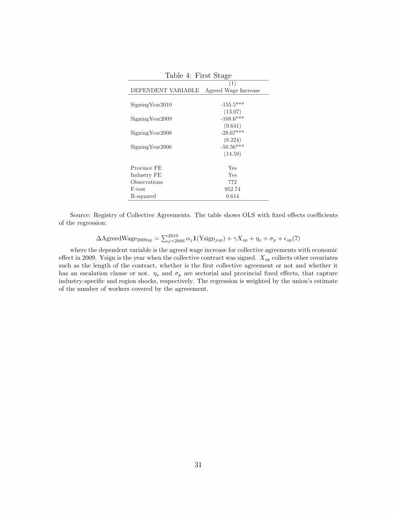
Table 4: First Stage(1)

DEPENDENT VARIABLE Agreed Wage Increase

SigningYear2010 -155.5***(13.07)

SigningYear2009 -108.6***(9.641)

SigningYear2008 -28.67***(8.224)

SigningYear2006 -50.56***(14.59)

Province FE YesIndustry FE YesObservations 772F-test 952.74R-squared 0.614

Source: Registry of Collective Agreements. The table shows OLS with fixed effects coefficientsof the regression:

∆AgreedWage2009sp =∑2010

j=2006 αj1(Ysignjsp) + γXsp + ηs + σp + εsp(7)

where the dependent variable is the agreed wage increase for collective agreements with economiceffect in 2009. Ysign is the year when the collective contract was signed. Xsp collects other covariatessuch as the length of the contract, whether is the first collective agreement or not and whether ithas an escalation clause or not. ηs and σp are sectorial and provincial fixed effects, that captureindustry-specific and region shocks, respectively. The regression is weighted by the union’s estimateof the number of workers covered by the agreeement.

31

Table 5: OLS estimates of the effects of year of signature on transitions to unemploymentUnempl. in 2009 +2010 2009 +2010 2009 +2010 2009 +2010Sample: All Low skilled All Low skilledSigned 2008 .0043 .0097 .0317** .0318** -.0016 .0086 .0492* .057**

(.0044) (.0061) (.0125) (.0145) (.0052) (.0078) (.027) (.029)

Age<30 .0326 .053 .063 .098 .032 .0528 .071 .104(.0057) (.0082) (.013) (.016) (.0057) (.0082) (.014) (.0169)

Age30-35 .0069 .0199 .0210 .064 .0066 0.019 .028 .067(.0042) (.006) (.016) (.019) (.0043) (.006) (.017) (.020)

Age36-40 -.0009 -.0003 .0054 .0092 -.001 -.0005 .011 .01(.004) (.0062) (.016) (.018) (.005) (.0062) (.017) (.018)

Age45-50 -.0038 -.00035 .0324 .035 -.0041 -.001 .039 .031(.0045) (.0056) (.0220) (.024) (.0045) (.006) (.024) (.025)

Age>50 .004 .02 .014 .029 .0043 .02 .020 .037(.004) (.006) (.021) (.023) (.0045) (.006) (.023) (.0247)

Low-skill .0405 .057 .040 .056(.00507) (.007) (.0052) (.007)

High-skill -.015 -0.0252 -0.0151 -0.0254(.006) (0.00785) (0.00603) (0.00799)

Fixed-term .158 .207 .182 .216 .158 0.21 .19 0.22(.013) (.013) (.015) (.019) (.013) (.013) (.015) (0.02)

Province FE yes yes yes yes yes yes yes yesIndustry FE yes yes yes yes yes yes yes yesRegion-year FE no no no no yes yes yes yesObservations 46,291 5,078 46,249 5,070R-squared 0.085 0.118 0.152 0.196 0.091 0.125 0.175 0.221

Robust standard errors in parentheses*** p<0.01, ** p<0.05, * p<0.1

Source: Registry of Collective Agreements and CSWH 2010, sample of men. The table shows OLSestimates of the regression:

P [U i(2009)|Ei(2008)] = 1(signed2008) +Xspi+µs+σp+εspi

The dependent variable takes value 1 if the individual lost his job during 2009-2010. Signed 2008 is a dummythat takes value one if the collective contract was signed in 2008. Xspi collects individual characteristicslike fixed-term contract, five age dummies, skill level and collective agreement characteristics - the lengthof the contract, whether is the first collective agreement and whether it has an escalation clause or not. µsand σp are sectorial and provincial fixed effects. Standard errors clustered at the 3digit industry-provincelevel.

Table 6A: The response of job loss to wage increases, full sample of males.First stage Intention to treat Two Stage Least Squares

(1) (2) (3) (4) (5)Dependent variable: Wage Increase P (U2009) P (U2009−2010) P (U2009) P (U2009−2010)Estimation method OLS OLS OLS TSLS TSLS1. Signed 2008 1.31*** .00430 0.00973

(.157) (.00436) (0.00611)2. Wage Increase .00328 .00742(agreed) (.0034) (.00491)

Province Fixed Effects yes yes yes yes yesIndustry Fixed Effects yes yes yes yes yesRegion*industry no no no no noObservations 46,291 46,291 46,291 46,291 46,291R-squared 0.712 0.085 0.118 0.085 0.117

Robust standard errors in parentheses*** p<0.01, ** p<0.05, * p<0.1

Source: Registry of Collective Agreements and CSWH 2010.Sample of males. The First Stage is esti-mated by OLS using the number of workers in Social Security sample as implicit weights. Wage increasesmeasured in percentage points.

AgreedWage2009 = α0+α11(SigningY ear2008sp) +Xspi+µs+σp+εspi

The Intention to Treat model regresses P (U2009), a shorthand for the probability of job loss P (U2009spi|E2008),on the same set of covariates

P (U2009spi|E2008) = β0+β11(signed2008sp) +Xspi+µs+σp+εspi

The main regression is an IV model of the probability of transition from employment to unemploymentas a function of the agreed wage increase, instrumenting the latter with the date of signature. Signed2008 isa dummy that takes value of one if the collective contract was signed in 2008. Xspi collects other covariatessuch as individual characteristics like type of contract (fixed-term contract), five age dummies, skill level,and collective agreement characteristics such as the length of the contract, whether is the first collectiveagreement or not and whether it has an escalation clause or not. µs and σp are 3-digit industry andprovincial fixed effects. Standard errors are clustered at the province-industry-level.

Table 6B: The response of job loss to wage increases, full sample males.(6) (7) (8) (9)

Dependent variable: Wage Increase P (U2009) P (U2009−2010) P (U2009) P (U2009−2010)Estimation method WLS OLS OLS TSLS TSLS1. Signed 2008 1.353*** -.00159 .0086

(.187) (.00521) (.0077)2. Wage Increase -.0016 .00626(agreed) (.0040) (.0059)

Province Fixed Effects yes yes yes yes yesIndustry Fixed Effects yes yes yes yes yesRegion*industry yes yes yes yes yesObservations 46,249 46,249 46,249 46,249 46,249R-squared 0.938 0.091 0.125 0.090 0.124

Robust standard errors in parentheses*** p<0.01, ** p<0.05, * p<0.1

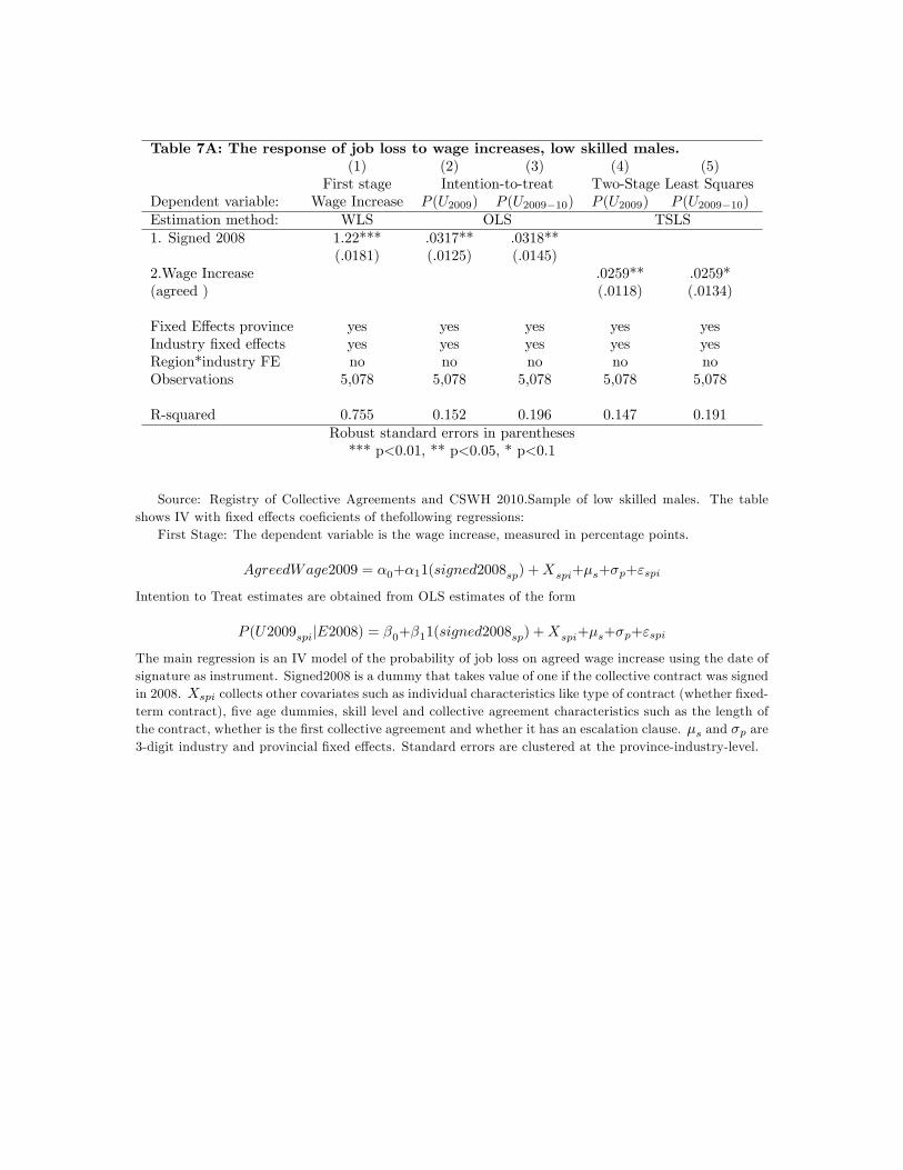
Table 7A: The response of job loss to wage increases, low skilled males.(1) (2) (3) (4) (5)

First stage Intention-to-treat Two-Stage Least SquaresDependent variable: Wage Increase P (U2009) P (U2009−10) P (U2009) P (U2009−10)Estimation method: WLS OLS TSLS1. Signed 2008 1.22*** .0317** .0318**

(.0181) (.0125) (.0145)2.Wage Increase .0259** .0259*(agreed ) (.0118) (.0134)

Fixed Effects province yes yes yes yes yesIndustry fixed effects yes yes yes yes yesRegion*industry FE no no no no noObservations 5,078 5,078 5,078 5,078 5,078

R-squared 0.755 0.152 0.196 0.147 0.191Robust standard errors in parentheses*** p<0.01, ** p<0.05, * p<0.1

Source: Registry of Collective Agreements and CSWH 2010.Sample of low skilled males. The tableshows IV with fixed effects coeficients of thefollowing regressions:

First Stage: The dependent variable is the wage increase, measured in percentage points.

AgreedWage2009 = α0+α11(signed2008sp) +Xspi+µs+σp+εspi

Intention to Treat estimates are obtained from OLS estimates of the form

P (U2009spi|E2008) = β0+β11(signed2008sp) +Xspi+µs+σp+εspi

The main regression is an IV model of the probability of job loss on agreed wage increase using the date ofsignature as instrument. Signed2008 is a dummy that takes value of one if the collective contract was signedin 2008. Xspi collects other covariates such as individual characteristics like type of contract (whether fixed-term contract), five age dummies, skill level and collective agreement characteristics such as the length ofthe contract, whether is the first collective agreement and whether it has an escalation clause. µs and σp are3-digit industry and provincial fixed effects. Standard errors are clustered at the province-industry-level.

Table 7B: The response of job loss to wage increases, low skilled males.(6) (7) (8) (9) (10)

First stage Intention-to-treat Two Stage Least SquaresDependent variable: Wage Increase P (U2009) P (U2009−2010) P (U2009) P (U2009−2010)Estimation method: WLS OLS TSLS1. Signed 2008 .954*** .0492* .0574**

(.020) (.0267) (.0289)2. Wage Increase .0516 .0602*(agreed) (.0318) (.0341)

Fixed Effects province yes yes yes yes yesIndustry fixed effects yes yes yes yes yesRegion*industry FE yes yes yes yes yesObservations 5,070 5,070 5,070 5,070 5,070

R-squared 0.950 0.175 0.221 0.171 0.219Robust standard errors in parentheses*** p<0.01, ** p<0.05, * p<0.1

Table 8: Job loss responses to signature date, by distance between wage and sectoral floor.No interactions Continous Discrete(1) (2) (3) (4)

Prob. Unemployment 2009 2009-2010 2009 2009-2010 2009 2009-2010

1. Signed 2008 .0243*** .0388*** .0431*** .0536*** .0423*** .0468***(.00914) (.0109) (.0119) (.0150) (.0145) (.0169)

2. Binding*Signed 2008 -.0028** -.00235(.0012) (.0015)

3. Binding -.00148** -.00374***(.00063) (.00072)

4. (300<Binding<1,000 euros) -.0257 -.0094*Signed 2008 (.0193) (.023)5. (Binding>1,000 euros)* -.0339** -.0214Signed 2008 (.017) (.0237)6. (300<Binding<1,000 euros) -.0402*** -.0677***

(.0152) (.0177)7. (Binding>1,000 euros) -.0429*** -.0807***

(.011) (.0121)Province + Industry F.E. yesRegion* Industry fixed effects noObservations 10,748 10,748 10,748 10,748 10,748 10,748R-squared 0.126 0.167 0.128 0.171 0.130 0.173

Robust standard errors in parentheses*** p<0.01, ** p<0.05, * p<0.1

Source: Registry of Collective Agreements and CSWH 2010. Sample of men with information oncollectively bargained wage levels. The information includes five industries only: Construction, Metal,Retail Trade, Accommodation and Food Service and Other Services and seven groups of the Spanish SocialSecurity System: 1, 2, 3 (High Skilled), 4, 5, 6 (Medium Skilled) and 10 (Low Skilled).

Binding = Nominal wage individual - Collective Agreement Wage (within industry, province and groupof skill).

Model in columns 1-4:

P (U2009spi|E2008spi)= δ 0+δ11(signed2008sp) + δ11(signed2008sp) ∗Binding+δ2Binding +Xspi+µs+σp+εspi

The dependent variable takes value 1 if the the individual transits from employment into unemployment in2009 (or 2010) conditional to be employed in 2008. Signed2008 is a dummy that takes value of one if thecollective contract was signed in 2008. Standard errors clustered at the province-3 digit industry level. Seenotes to tables 5-7.

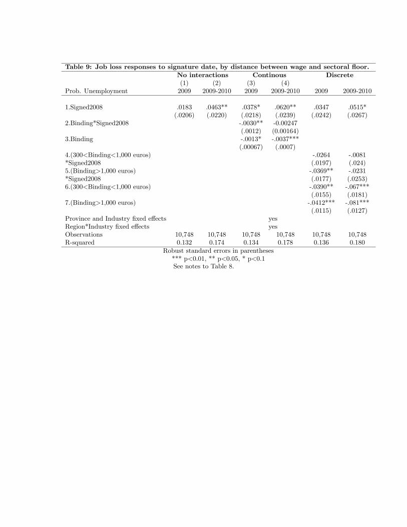
Table 9: Job loss responses to signature date, by distance between wage and sectoral floor.No interactions Continous Discrete(1) (2) (3) (4)

Prob. Unemployment 2009 2009-2010 2009 2009-2010 2009 2009-2010

1.Signed2008 .0183 .0463** .0378* .0620** .0347 .0515*(.0206) (.0220) (.0218) (.0239) (.0242) (.0267)

2.Binding*Signed2008 -.0030** -0.00247(.0012) (0.00164)

3.Binding -.0013* -.0037***(.00067) (.0007)

4.(300<Binding<1,000 euros) -.0264 -.0081*Signed2008 (.0197) (.024)5.(Binding>1,000 euros) -.0369** -.0231*Signed2008 (.0177) (.0253)6.(300<Binding<1,000 euros) -.0390** -.067***

(.0155) (.0181)7.(Binding>1,000 euros) -.0412*** -.081***

(.0115) (.0127)Province and Industry fixed effects yesRegion*Industry fixed effects yesObservations 10,748 10,748 10,748 10,748 10,748 10,748R-squared 0.132 0.174 0.134 0.178 0.136 0.180

Robust standard errors in parentheses*** p<0.01, ** p<0.05, * p<0.1See notes to Table 8.

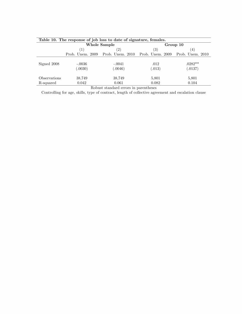
Table 10. The response of job loss to date of signature, females.Whole Sample Group 10

(1) (2) (3) (4)Prob. Unem. 2009 Prob. Unem. 2010 Prob. Unem. 2009 Prob. Unem. 2010

Signed 2008 -.0036 -.0041 .012 .0282**(.0030) (.0046) (.013) (.0137)

Observations 38,749 38,749 5,801 5,801R-squared 0.042 0.061 0.082 0.104

Robust standard errors in parenthesesControlling for age, skills, type of contract, length of collective agreement and escalation clause

Table 11: Job loss responses to signature date, by distance between wage and sectoral floor.Sample of newly hired males

No interactions Continous Discrete(1) (2) (3) (4)

Prob. Unemployment 2009 2009-2010 2009 2009-2010 2009 2009-2010

1. Signed2008 .0235 .0380 .0473** .0805*** .0596** .0653**(.0187) (.0232) (.0236) (.0306) (.0262) (.0299)

2. Binding*Signed2008 -0.00416 -.00738**(.00271) (.00313)

3. Binding -.000781 -.00088(.00158) (.002)

4. (300<Binding<1,000 euros) -.0809** -.0183*Signed 2008 (.0403) (.0439)5. (Binding>1,000 euros) -.0497 -.0951***Signed 2008 (.0429) (.0462)6. (300<Binding<1,000 euros) -.0117 -.0313

(.0251) (.0250)7. (Binding>1,000 euros) -.0207 -.0285

(.0193) (.0262)Province and industry fixed-effects yesRegion*Industry fixed effects noObservations 1,893 1,893 1,893 1,893 1,893 1,893R-squared 0.174 0.219 0.176 0.223 0.178 0.223

Robust standard errors in parentheses*** p<0.01, ** p<0.05, * p<0.1