Fluid Flow 2.9

For fully developed laminar-viscous flow in a pipe, the loss isevaluated from Equation (8) as follows:

(27)

where Thus, for laminar flow, thefriction factor varies inversely with the Reynolds number.

With turbulent flow, friction loss depends not only on flow con-ditions, as characterized by the Reynolds number, but also on thenature of the conduit wall surface. For smooth conduit walls, empir-ical correlations give

(28a)

(28b)

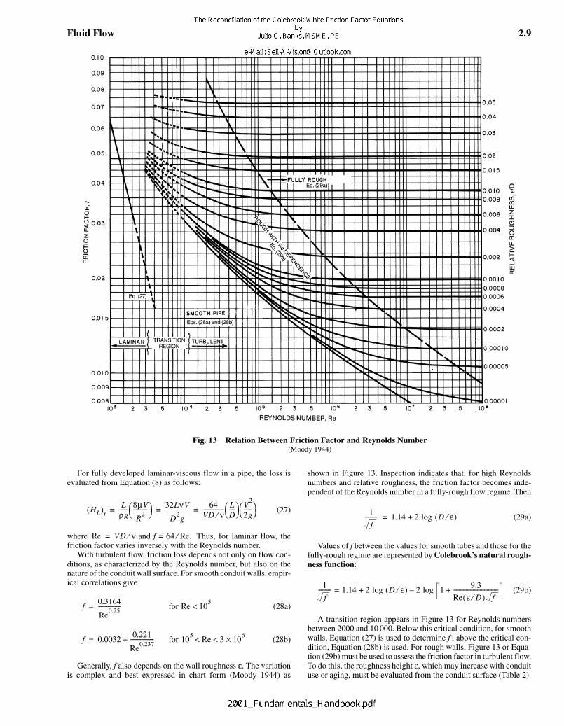
Generally, f also depends on the wall roughness ε. The variationis complex and best expressed in chart form (Moody 1944) as

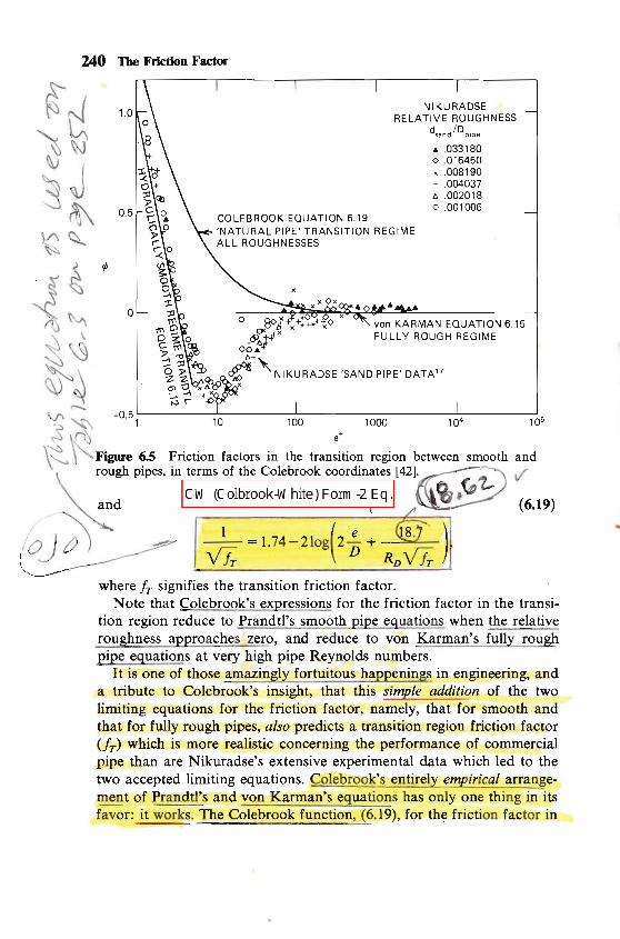
shown in Figure 13. Inspection indicates that, for high Reynoldsnumbers and relative roughness, the friction factor becomes inde-pendent of the Reynolds number in a fully-rough flow regime. Then

(29a)

Values of f between the values for smooth tubes and those for thefully-rough regime are represented by Colebrook’s natural rough-ness function:

(29b)

A transition region appears in Figure 13 for Reynolds numbersbetween 2000 and 10 000. Below this critical condition, for smoothwalls, Equation (27) is used to determine f ; above the critical con-dition, Equation (28b) is used. For rough walls, Figure 13 or Equa-tion (29b) must be used to assess the friction factor in turbulent flow.To do this, the roughness height ε, which may increase with conduituse or aging, must be evaluated from the conduit surface (Table 2).

Fig. 13 Relation Between Friction Factor and Reynolds Number(Moody 1944)

HL( )f

Lρg------ 8µV

R2

---------- 32LνV

D2g

----------------- 64VD ν⁄--------------- L

D----

V2

2g------

= = =

Re VD ν and f 64 Re.⁄=⁄=

f0.3164

Re0.25

----------------= for Re 105<

f 0.00320.221

Re0.237

-----------------+= for 105

Re 3< < 106×

1

f --------- 1.14 2 log D ε⁄( )+=

1

f --------- 1.14 2 log D ε⁄( )+= 2 log 1

9.3

Re ε D⁄( ) f --------------------------------+–

Colebrook-White Friction Factor Equation Derivation 1 of 3.mcdx Page 1 of 2

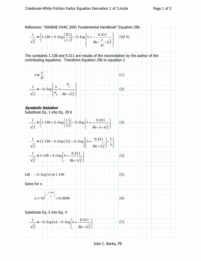
Reference: "ASHRAE HVAC 2001 Fundamental Handbook" Equation 29b

＝――1

‾f−

⎛⎜⎝

+1.138 ⋅2 log⎛⎜⎝―D

ε

⎞⎟⎠

⎞⎟⎠

⋅2 log⎛⎜⎜⎝

+1 ――――9.311

⋅⋅Re ―ε

D‾‾f

⎞⎟⎟⎠

((29 b))

The constants 1.138 and 9.311 are results of the reconciliation by the author of the contributing equations. Transform Equation 29b to equation 2

＝λ ―ε

D((1))

＝――1

‾f⋅−2 log

⎛⎜⎜⎝

+―λ

a0

―――

b0

⋅Re ‾f

⎞⎟⎟⎠

((2))

Symbolic SolutionSubstitute Eq. 1 into Eq. 29 b

＝――1

‾f−

⎛⎜⎝

+1.138 ⋅2 log⎛⎜⎝―1

λ

⎞⎟⎠

⎞⎟⎠

⋅2 log⎛⎜⎝+1 ――――

9.311

⋅⋅Re λ ‾‾f

⎞⎟⎠

((3))

＝――1

‾f−(( −1.138 ⋅2 log ((λ)))) ⋅2 log

⎛⎜⎝

⋅⎛⎜⎝+λ ―――

9.311

⋅Re ‾‾f

⎞⎟⎠―1

λ

⎞⎟⎠

＝――1

‾f−1.138 ⋅2 log

⎛⎜⎝+λ ―――

9.311

⋅Re ‾‾f

⎞⎟⎠

((4))

Let ＝⋅−2 log ((x)) 1.138 ((5))

Solve for x

≔x =10

⎛⎜⎝−――1.138

2

⎞⎟⎠0.2698 ((6))

Substitute Eq. 5 into Eq. 4

＝――1

‾f−⋅−2 log ((x)) ⋅2 log

⎛⎜⎝+λ ―――

9.311

⋅Re ‾‾f

⎞⎟⎠

((7))

Julio C. Banks, PE

Colebrook-White Friction Factor Equation Derivation 1 of 3.mcdx Page 2 of 2

＝――1

‾f⋅−2 log

⎛⎜⎝

+⋅λ x ―――⋅9.311 x

⋅Re ‾‾f

⎞⎟⎠

((8))

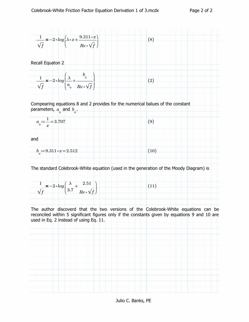
Recall Equaton 2

＝――1

‾f⋅−2 log

⎛⎜⎜⎝

+―λ

a0

―――

b0

⋅Re ‾f

⎞⎟⎟⎠

((2))

Compearing equations 8 and 2 provides for the numerical balues of the constant parameters, and .a

0b0

≔a0

=―1

x3.707 ((9))

and

≔b0

=⋅9.311 x 2.512 ((10))

The standard Colebrook-White equation (used in the generation of the Moody Diagram) is

＝――1

‾f⋅−2 log

⎛⎜⎝

+――λ

3.7―――2.51

⋅Re ‾‾f

⎞⎟⎠

((11))

The author discoverd that the two versions of the Colebrook-White equations can be reconciled within 5 significant figures only if the constants given by equations 9 and 10 are used in Eq. 2 instead of using Eq. 11.

Julio C. Banks, PE

Colebrook-White Friction Factor Equation Derivation 2 of 3.mcdx Page 1 of 2

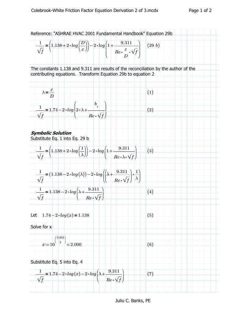
Reference: "ASHRAE HVAC 2001 Fundamental Handbook" Equation 29b

＝――1

‾f−

⎛⎜⎝

+1.138 ⋅2 log⎛⎜⎝―D

ε

⎞⎟⎠

⎞⎟⎠

⋅2 log⎛⎜⎜⎝

+1 ――――9.311

⋅⋅Re ―ε

D‾‾f

⎞⎟⎟⎠

((29 b))

The constants 1.138 and 9.311 are results of the reconciliation by the author of the contributing equations. Transform Equation 29b to equation 2

＝λ ―ε

D((1))

＝――1

‾f−1.74 ⋅2 log

⎛⎜⎜⎝

+⋅2 λ ―――

b1

⋅Re ‾‾f

⎞⎟⎟⎠

((2))

Symbolic SolutionSubstitute Eq. 1 into Eq. 29 b

＝――1

‾f−

⎛⎜⎝

+1.138 ⋅2 log⎛⎜⎝―1

λ

⎞⎟⎠

⎞⎟⎠

⋅2 log⎛⎜⎝

+1 ――――9.311

⋅⋅Re λ ‾‾f

⎞⎟⎠

((3))

＝――1

‾f−(( −1.138 ⋅2 log ((λ)))) ⋅2 log

⎛⎜⎝

⋅⎛⎜⎝

+λ ―――9.311

⋅Re ‾‾f

⎞⎟⎠

―1

λ

⎞⎟⎠

＝――1

‾f−1.138 ⋅2 log

⎛⎜⎝

+λ ―――9.311

⋅Re ‾‾f

⎞⎟⎠

((4))

Let ＝−1.74 ⋅2 log ((x)) 1.138 ((5))

Solve for x

≔x =10

⎛⎜⎝――0.602

2

⎞⎟⎠

2.000 ((6))

Substitute Eq. 5 into Eq. 4

＝――1

‾f−−1.74 ⋅2 log ((x)) ⋅2 log

⎛⎜⎝

+λ ―――9.311

⋅Re ‾‾f

⎞⎟⎠

((7))

Julio C. Banks, PE

Colebrook-White Friction Factor Equation Derivation 2 of 3.mcdx Page 2 of 2

＝――1

‾f−1.74 ⋅2 log

⎛⎜⎝

+⋅x λ ―――⋅9.311 x

⋅Re ‾f

⎞⎟⎠

((8))

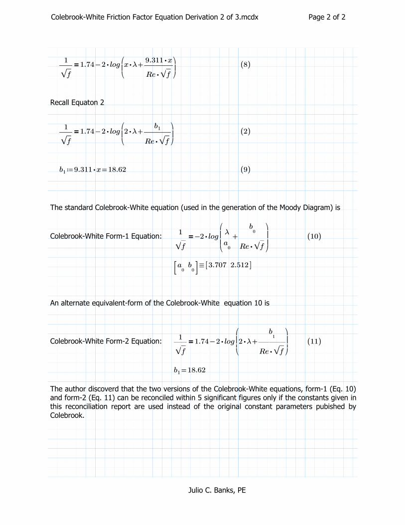
Recall Equaton 2

＝――1

‾f−1.74 ⋅2 log

⎛⎜⎝

+⋅2 λ ―――b1

⋅Re ‾‾f

⎞⎟⎠

((2))

≔b1 =⋅9.311 x 18.62 ((9))

The standard Colebrook-White equation (used in the generation of the Moody Diagram) is

Colebrook-White Form-1 Equation: ＝――1

‾f⋅−2 log

⎛⎜⎜⎝

+―λ

a0

―――

b0

⋅Re ‾f

⎞⎟⎟⎠

((10))

≡a0b

0⎡⎣

⎤⎦

3.707 2.512[[ ]]

An alternate equivalent-form of the Colebrook-White equation 10 is

Colebrook-White Form-2 Equation: ＝――1

‾f−1.74 ⋅2 log

⎛⎜⎜⎝

+⋅2 λ ―――

b1

⋅Re ‾‾f

⎞⎟⎟⎠

((11))

=b1 18.62

The author discoverd that the two versions of the Colebrook-White equations, form-1 (Eq. 10) and form-2 (Eq. 11) can be reconciled within 5 significant figures only if the constants given in this reconciliation report are used instead of the original constant parameters pubished by Colebrook.

Julio C. Banks, PE

Colebrook-White Friction Factor Equation Derivation 3 of 3.mcdx Page 1 of 5

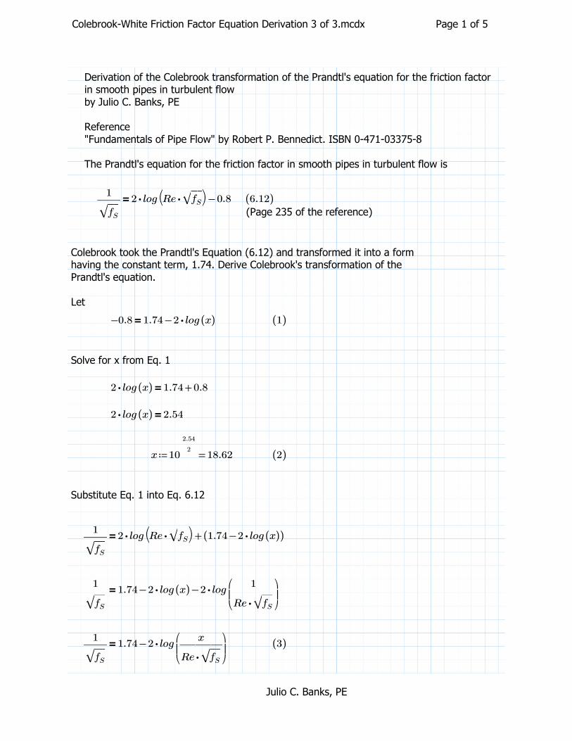
Derivation of the Colebrook transformation of the Prandtl's equation for the friction factor in smooth pipes in turbulent flowby Julio C. Banks, PE

Reference"Fundamentals of Pipe Flow" by Robert P. Bennedict. ISBN 0-471-03375-8

The Prandtl's equation for the friction factor in smooth pipes in turbulent flow is

＝――1

‾‾fS

−⋅2 log⎛⎝ ⋅Re ‾‾fS

⎞⎠ 0.8 ((6.12))

(Page 235 of the reference)

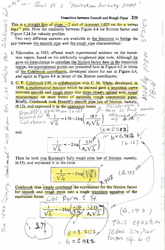
Colebrook took the Prandtl's Equation (6.12) and transformed it into a form having the constant term, 1.74. Derive Colebrook's transformation of the Prandtl's equation.

Let

＝−0.8 −1.74 ⋅2 log ((x)) ((1))

Solve for x from Eq. 1

＝⋅2 log ((x)) +1.74 0.8

＝⋅2 log ((x)) 2.54

≔x =10――2.54

218.62 ((2))

Substitute Eq. 1 into Eq. 6.12

＝――1

‾‾fS

+⋅2 log⎛⎝ ⋅Re ‾‾fS

⎞⎠ (( −1.74 ⋅2 log ((x))))

＝――1

‾‾fS

−−1.74 ⋅2 log ((x)) ⋅2 log⎛⎜⎝―――

1

⋅Re ‾‾fS

⎞⎟⎠

＝――1

‾‾fS

−1.74 ⋅2 log⎛⎜⎝―――

x

⋅Re ‾‾fS

⎞⎟⎠

((3))

Julio C. Banks, PE

Colebrook-White Friction Factor Equation Derivation 3 of 3.mcdx Page 2 of 5

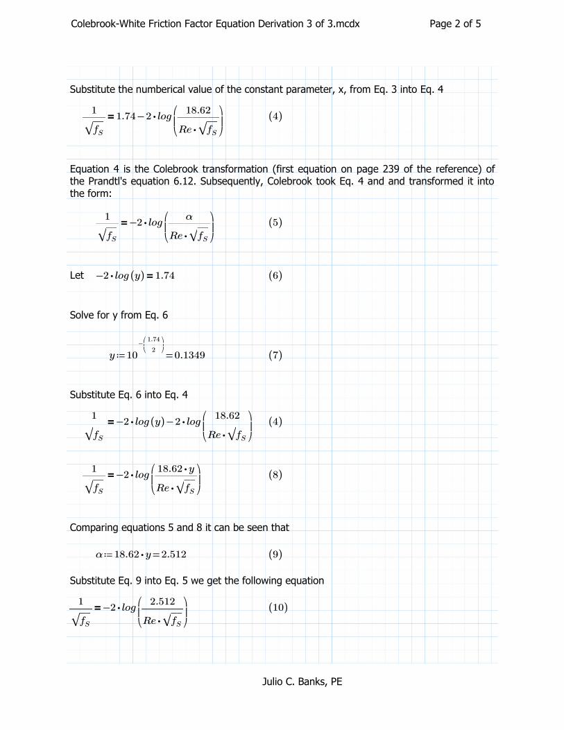
Substitute the numberical value of the constant parameter, x, from Eq. 3 into Eq. 4

＝――1

‾‾fS

−1.74 ⋅2 log⎛⎜⎝―――18.62

⋅Re ‾‾fS

⎞⎟⎠

((4))

Equation 4 is the Colebrook transformation (first equation on page 239 of the reference) of the Prandtl's equation 6.12. Subsequently, Colebrook took Eq. 4 and and transformed it into the form:

＝――1

‾‾fS

⋅−2 log⎛⎜⎝―――

α

⋅Re ‾‾fS

⎞⎟⎠

((5))

Let ＝⋅−2 log ((y)) 1.74 ((6))

Solve for y from Eq. 6

≔y =10−⎛⎜⎝――1.74

2

⎞⎟⎠0.1349 ((7))

Substitute Eq. 6 into Eq. 4

＝――1

‾‾fS

−⋅−2 log ((y)) ⋅2 log⎛⎜⎝―――18.62

⋅Re ‾‾fS

⎞⎟⎠

((4))

＝――1

‾‾fS

⋅−2 log⎛⎜⎝―――

⋅18.62 y

⋅Re ‾‾fS

⎞⎟⎠

((8))

Comparing equations 5 and 8 it can be seen that

≔α =⋅18.62 y 2.512 ((9))

Substitute Eq. 9 into Eq. 5 we get the following equation

＝――1

‾‾fS

⋅−2 log⎛⎜⎝―――2.512

⋅Re ‾‾fS

⎞⎟⎠

((10))

Julio C. Banks, PE

Colebrook-White Friction Factor Equation Derivation 3 of 3.mcdx Page 3 of 5

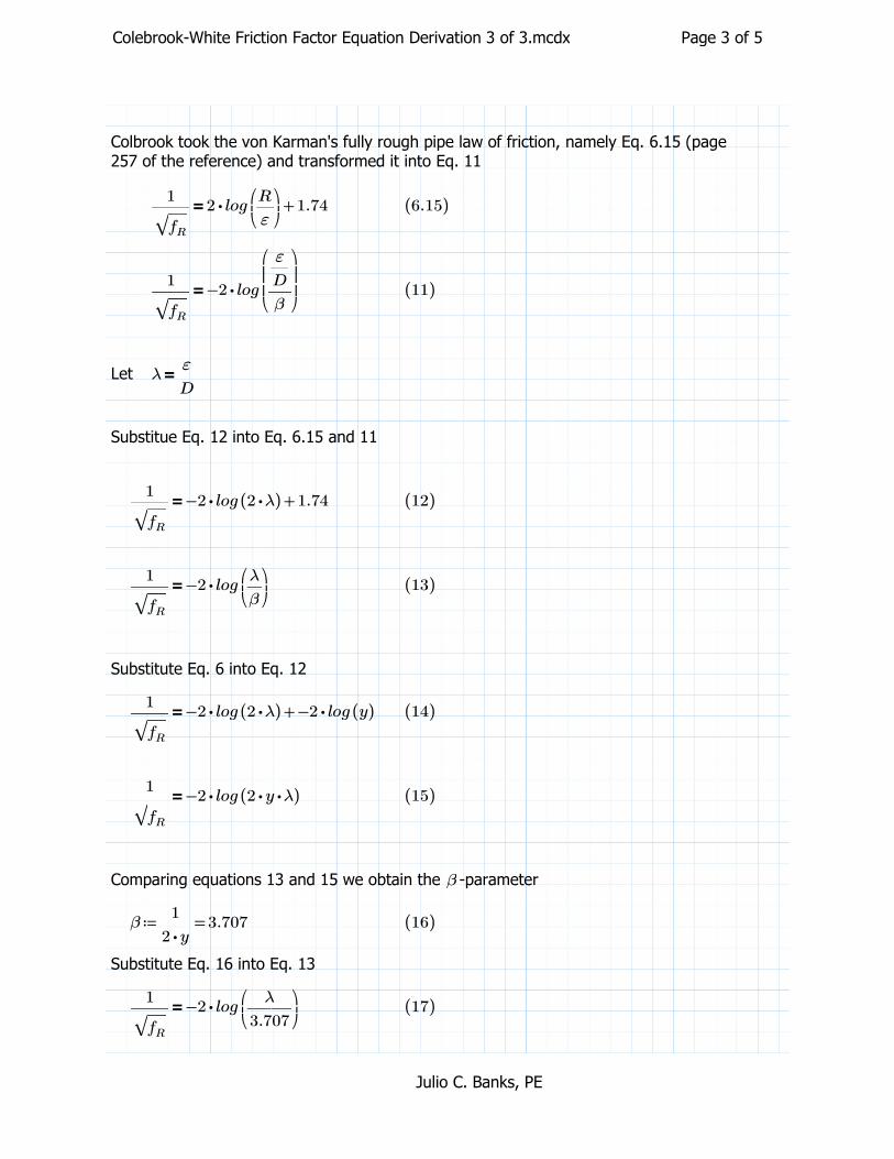
Colbrook took the von Karman's fully rough pipe law of friction, namely Eq. 6.15 (page 257 of the reference) and transformed it into Eq. 11

＝――1

‾‾fR

+⋅2 log⎛⎜⎝―R

ε

⎞⎟⎠

1.74 ((6.15))

＝――1

‾‾fR

⋅−2 log

⎛⎜⎜⎝―

―ε

D

β

⎞⎟⎟⎠

((11))

Let ＝λ ―ε

D

Substitue Eq. 12 into Eq. 6.15 and 11

＝――1

‾‾fR

+⋅−2 log (( ⋅2 λ)) 1.74 ((12))

＝――1

‾‾fR

⋅−2 log⎛⎜⎝―λ

β

⎞⎟⎠

((13))

Substitute Eq. 6 into Eq. 12

＝――1

‾‾fR

+⋅−2 log (( ⋅2 λ)) ⋅−2 log ((y)) ((14))

＝――1

‾‾fR

⋅−2 log (( ⋅⋅2 y λ)) ((15))

Comparing equations 13 and 15 we obtain the -parameterβ

≔β =――1

⋅2 y3.707 ((16))

Substitute Eq. 16 into Eq. 13

＝――1

‾‾fR

⋅−2 log⎛⎜⎝――λ

3.707

⎞⎟⎠

((17))

Julio C. Banks, PE

Colebrook-White Friction Factor Equation Derivation 3 of 3.mcdx Page 4 of 5

Colebrook then took equations 5 and 13 and combined them into a single expression

＝――1

‾‾fS

⋅−2 log⎛⎜⎝―――

α

⋅Re ‾‾fS

⎞⎟⎠

((5))

≔α =⋅18.62 y 2.512 ((9))

＝――1

‾‾fR

⋅−2 log⎛⎜⎝―λ

β

⎞⎟⎠

((13))

≔β =――1

⋅2 y3.707 ((16))

Solve for the arguments of the logarithms for subsequent combination

＝10

⎛⎜⎝

――――1

⋅−2 ‾‾‾fR

⎞⎟⎠―λ

β((17))

＝10

⎛⎜⎝

――――1

⋅−2 ‾‾fS

⎞⎟⎠―――

α

⋅Re ‾‾fS

((18))

Add equations 17 and 18

＝+10

⎛⎜⎝

――――1

⋅−2 ‾‾‾fR

⎞⎟⎠10

⎛⎜⎝

――――1

⋅−2 ‾‾fS

⎞⎟⎠

+―λ

β―――

α

⋅Re ‾‾fS

((19))

Let ＝10

⎛⎜⎝

――――1

⋅−2 ‾‾fT

⎞⎟⎠

+10

⎛⎜⎝

――――1

⋅−2 ‾‾fR

⎞⎟⎠10

⎛⎜⎝

――――1

⋅−2 ‾‾fS

⎞⎟⎠

((20))

Where is the Transition Friction Factor.fT

Substitute Eq. 20 into Eq. 19

＝10

⎛⎜⎝

――――1

⋅−2 ‾‾fT

⎞⎟⎠

+―λ

β―――

α

⋅Re ‾‾fT

((21))

Julio C. Banks, PE

Colebrook-White Friction Factor Equation Derivation 3 of 3.mcdx Page 5 of 5

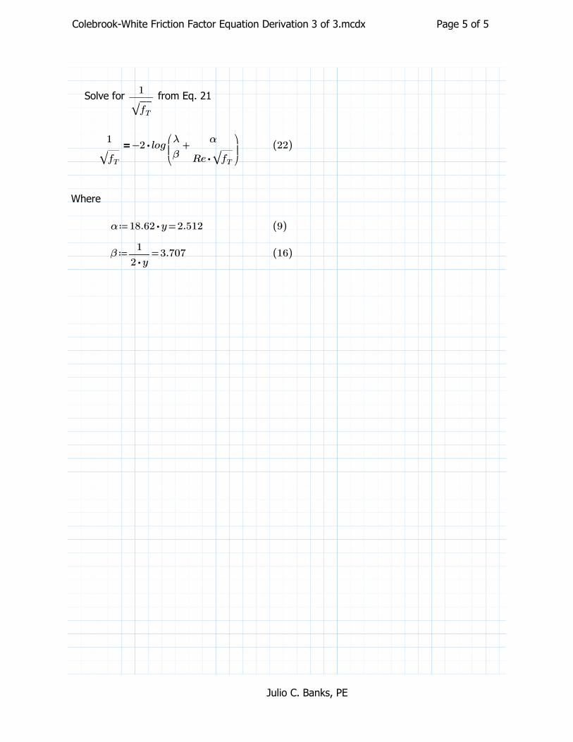
Solve for from Eq. 21――1

‾‾fT

＝――1

‾‾fT

⋅−2 log⎛⎜⎝

+―λ

β―――

α

⋅Re ‾‾fT

⎞⎟⎠

((22))

Where

≔α =⋅18.62 y 2.512 ((9))

≔β =――1

⋅2 y3.707 ((16))

Julio C. Banks, PE

FUNDAMENTALS OF

PIPE FLOW Julio e. :Bank:S.

Robert P. Benedict

Fellow Mechanical Engineer Westinghouse Electric Corporation

Steam Turbine Division Adjunct Professor of Mechanical Engineering

Drexel University Evening College

Philadelphia, Pennsylvania

A WILEY-INTERSCIENCE PUBLICATION

JOHN WILEY & SONS

New York • Chichester • Brisbane • Toronto • Singapore

3

BanksJ

Rectangle