cody's data cleaning techniques using sas®, third edition · chapter 4: data cleaning...

Contents

List of Programs ................................................................................................ ix

About This Book ................................................................................................ xv

About The Author ............................................................................................ xvii

Acknowledgments ............................................................................................ xix

Introduction ..................................................................................................... xxi

Chapter 1: Working with Character Data ........................................................... 1

Introduction .............................................................................................................................................. 1 Using PROC FREQ to Detect Character Variable Errors ..................................................................... 4 Changing the Case of All Character Variables in a Data Set .............................................................. 6 A Summary of Some Character Functions (Useful for Data Cleaning) .............................................. 8

UPCASE, LOWCASE, and PROPCASE ............................................................................................ 8 NOTDIGIT, NOTALPHA, and NOTALNUM ....................................................................................... 8 VERIFY ................................................................................................................................................ 9 COMPBL ............................................................................................................................................. 9 COMPRESS ........................................................................................................................................ 9 MISSING ........................................................................................................................................... 10 TRIMN and STRIP ............................................................................................................................ 10

Checking that a Character Value Conforms to a Pattern .................................................................. 11 Using a DATA Step to Detect Character Data Errors ........................................................................ 12 Using PROC PRINT with a WHERE Statement to Identify Data Errors ............................................ 13 Using Formats to Check for Invalid Values ......................................................................................... 14 Creating Permanent Formats ............................................................................................................... 16 Removing Units from a Value ............................................................................................................... 17 Removing Non-Printing Characters from a Character Value ............................................................ 18 Conclusions ............................................................................................................................................ 19

Chapter 2: Using Perl Regular Expressions to Detect Data Errors ................... 21 Introduction ............................................................................................................................................ 21 Describing the Syntax of Regular Expressions .................................................................................. 21 Checking for Valid ZIP Codes and Canadian Postal Codes .............................................................. 23 Searching for Invalid Email Addresses ................................................................................................ 25 Verifying Phone Numbers ..................................................................................................................... 26

From Cody's Data Cleaning Techniques Using SAS®, Third Edition. Full book available for purchase here.

http://www.sas.com/store/prodBK_70074_en.html

iv

Converting All Phone Numbers to a Standard Form .......................................................................... 27 Developing a Macro to Test Regular Expressions ............................................................................. 28 Conclusions ............................................................................................................................................ 29

Chapter 3: Standardizing Data ......................................................................... 31

Introduction ............................................................................................................................................ 31 Using Formats to Standardize Company Names ............................................................................... 31 Creating a Format from a SAS Data Set .............................................................................................. 33 Using TRANWRD and Other Functions to Standardize Addresses .................................................. 36 Using Regular Expressions to Help Standardize Addresses............................................................. 38 Performing a "Fuzzy" Match between Two Files ................................................................................ 40 Conclusions ............................................................................................................................................ 44

Chapter 4: Data Cleaning Techniques for Numeric Data .................................. 45 Introduction ............................................................................................................................................ 45 Using PROC UNIVARIATE to Examine Numeric Variables ................................................................ 45 Describing an ODS Option to List Selected Portions of the Output ................................................. 49 Listing Output Objects Using the Statement TRACE ON .................................................................. 52 Using a PROC UNIVARIATE Option to List More Extreme Values .................................................... 52 Presenting a Program to List the 10 Highest and Lowest Values..................................................... 53 Presenting a Macro to List the n Highest and Lowest Values .......................................................... 55 Describing Two Programs to List the Highest and Lowest Values by Percentage ........................ 58

Using PROC UNIVARIATE ............................................................................................................... 58 Presenting a Macro to List the Highest and Lowest n% Values ................................................ 60 Using PROC RANK .......................................................................................................................... 62

Using Pre-Determined Ranges to Check for Possible Data Errors .................................................. 66 Identifying Invalid Values versus Missing Values ............................................................................... 67 Checking Ranges for Several Variables and Generating a Single Report ....................................... 69 Conclusions ............................................................................................................................................ 72

Chapter 5: Automatic Outlier Detection for Numeric Data ................................ 73

Introduction ............................................................................................................................................ 73 Automatic Outlier Detection (Using Means and Standard Deviations) ............................................ 73 Detecting Outliers Based on a Trimmed Mean and Standard Deviation ......................................... 75 Describing a Program that Uses Trimmed Statistics for Multiple Variables ................................... 78 Presenting a Macro Based on Trimmed Statistics ............................................................................. 81 Detecting Outliers Based on the Interquartile Range ........................................................................ 83 Conclusions ............................................................................................................................................ 86

v

Chapter 6: More Advanced Techniques for Finding Errors in Numeric Data .... 87

Introduction ............................................................................................................................................ 87 Introducing the Banking Data Set ........................................................................................................ 87 Running the Auto_Outliers Macro on Bank Deposits ........................................................................ 91 Identifying Outliers Within Each Account ............................................................................................ 92 Using Box Plots to Inspect Suspicious Deposits ............................................................................... 95 Using Regression Techniques to Identify Possible Errors in the Banking Data ............................. 99 Using Regression Diagnostics to Identify Outliers .......................................................................... 104 Conclusions .......................................................................................................................................... 108

Chapter 7: Describing Issues Related to Missing and Special Values (Such as 999) ................................................................................ 109

Introduction .......................................................................................................................................... 109 Inspecting the SAS Log ....................................................................................................................... 109 Using PROC MEANS and PROC FREQ to Count Missing Values ................................................... 110

Counting Missing Values for Numeric Variables ........................................................................ 110 Counting Missing Values for Character Variables ..................................................................... 111

Using DATA Step Approaches to Identify and Count Missing Values ........................................... 113 Locating Patient Numbers for Records Where Patno Is Either Missing or Invalid ....................... 113 Searching for a Specific Numeric Value ............................................................................................ 117 Creating a Macro to Search for Specific Numeric Values ............................................................... 119 Converting Values Such as 999 to a SAS Missing Value ................................................................. 121 Conclusions .......................................................................................................................................... 121

Chapter 8: Working with SAS Dates ............................................................... 123 Introduction .......................................................................................................................................... 123 Changing the Storage Length for SAS Dates ................................................................................... 123 Checking Ranges for Dates (Using a DATA Step) ............................................................................ 124 Checking Ranges for Dates (Using PROC PRINT) ........................................................................... 125 Checking for Invalid Dates .................................................................................................................. 125 Working with Dates in Nonstandard Form ........................................................................................ 128 Creating a SAS Date When the Day of the Month Is Missing .......................................................... 129 Suspending Error Checking for Known Invalid Dates ..................................................................... 131 Conclusions .......................................................................................................................................... 131

Chapter 9: Looking for Duplicates and Checking Data with Multiple Observations per Subject ............................................................. 133

Introduction .......................................................................................................................................... 133 Eliminating Duplicates by Using PROC SORT .................................................................................. 133

vi

Demonstrating a Possible Problem with the NODUPRECS Option ................................................ 136 Reviewing First. and Last. Variables .................................................................................................. 138 Detecting Duplicates by Using DATA Step Approaches .................................................................. 140 Using PROC FREQ to Detect Duplicate IDs ...................................................................................... 141 Working with Data Sets with More Than One Observation per Subject ........................................ 143 Identifying Subjects with n Observations Each (DATA Step Approach) ........................................ 144 Identifying Subjects with n Observations Each (Using PROC FREQ) ............................................. 146 Conclusions .......................................................................................................................................... 146

Chapter 10: Working with Multiple Files ......................................................... 147 Introduction .......................................................................................................................................... 147 Checking for an ID in Each of Two Files ............................................................................................ 147 Checking for an ID in Each of n Files ................................................................................................. 150 A Macro for ID Checking ..................................................................................................................... 152 Conclusions .......................................................................................................................................... 154

Chapter 11: Using PROC COMPARE to Perform Data Verification .................. 155

Introduction .......................................................................................................................................... 155 Conducting a Simple Comparison of Two Data Files ...................................................................... 155 Simulating Double Entry Verification Using PROC COMPARE ....................................................... 160 Other Features of PROC COMPARE .................................................................................................. 161 Conclusions .......................................................................................................................................... 162

Chapter 12: Correcting Errors ........................................................................ 163

Introduction .......................................................................................................................................... 163 Hard Coding Corrections .................................................................................................................... 163 Describing Named Input ...................................................................................................................... 164 Reviewing the UPDATE Statement .................................................................................................... 166 Using the UPDATE Statement to Correct Errors in the Patients Data Set .................................... 168 Conclusions .......................................................................................................................................... 171

Chapter 13: Creating Integrity Constraints and Audit Trails ........................... 173 Introduction .......................................................................................................................................... 173 Demonstrating General Integrity Constraints ................................................................................... 174 Describing PROC APPEND ................................................................................................................. 177 Demonstrating How Integrity Constraints Block the Addition of Data Errors .............................. 178 Adding Your Own Messages to Violations of an Integrity Constraint ............................................ 179 Deleting an Integrity Constraint Using PROC DATASETS ............................................................... 180 Creating an Audit Trail Data Set ......................................................................................................... 180

vii

Demonstrating an Integrity Constraint Involving More Than One Variable ................................... 183 Demonstrating a Referential Constraint ........................................................................................... 186 Attempting to Delete a Primary Key When a Foreign Key Still Exists ............................................ 188 Attempting to Add a Name to the Child Data Set ............................................................................. 190 Demonstrating How to Delete a Referential Constraint .................................................................. 191 Demonstrating the CASCADE Feature of a Referential Constraint ................................................ 191 Demonstrating the SET NULL Feature of a Referential Constraint ................................................ 192 Conclusions .......................................................................................................................................... 193

Chapter 14: A Summary of Useful Data Cleaning Macros ............................... 195 Introduction .......................................................................................................................................... 195 A Macro to Test Regular Expressions ............................................................................................... 195 A Macro to List the n Highest and Lowest Values of a Variable ..................................................... 196 A Macro to List the n% Highest and Lowest Values of a Variable ................................................. 197 A Macro to Perform Range Checks on Several Variables ............................................................... 198 A Macro that Uses Trimmed Statistics to Automatically Search for Outliers ............................... 200 A Macro to Search a Data Set for Specific Values Such as 999 ..................................................... 202 A Macro to Check for ID Values in Multiple Data Sets .................................................................... 203 Conclusions .......................................................................................................................................... 204

Index .............................................................................................................. 205

From Cody's Data Cleaning Techniques Using SAS®, Third Edition by Ron Cody. Copyright © 2017, SAS Institute Inc., Cary, North Carolina, USA. ALL RIGHTS RESERVED.


Chapter 5: Automatic Outlier Detection for Numeric Data

Introduction .................................................................................................................................73

Automatic Outlier Detection (Using Means and Standard Deviations) ...........................................73

Detecting Outliers Based on a Trimmed Mean and Standard Deviation ........................................75

Describing a Program that Uses Trimmed Statistics for Multiple Variables ..................................78

Presenting a Macro Based on Trimmed Statistics ........................................................................81

Detecting Outliers Based on the Interquartile Range ...................................................................83

Conclusions .................................................................................................................................86

Introduction As you saw in the previous chapter, there are many variables where it is possible to specify a reasonable range for numeric values. When this is not possible, there are other tools in the data cleaning toolbox that you can use. Many of these methods look at the distribution of data values and identify values that appear to be outliers. (Note: In epidemiology, there are certain variables such as age or weight where you might have outright liars.)

Automatic Outlier Detection (Using Means and Standard Deviations) If your data values have a distribution that looks similar to a normal distribution or at least is somewhat symmetrical (as determined by statistical techniques such as computing skewness and kurtosis or inspection of a histogram of the data), you might consider using properties of the distribution to help identify possible data errors. For example, you could decide to flag all values more than two standard deviations from the mean. However, if you had some severe data errors, the standard deviation could be so badly inflated that obviously incorrect data values might lie within two standard deviations of the mean (and not be identified as possible errors).

A possible workaround for this would be to compute the standard deviation after removing some of the highest and lowest values. For example, you could compute a standard deviation of the middle 80% of your data and use this to decide on outliers. Another popular alternative is to use an algorithm based on the interquartile range (the difference between the 25th percentile and the 75th percentile).

Let's first see how you could identify data values more than two standard deviations from the mean. You can use PROC MEANS to compute the mean and standard deviation, followed by a short DATA step to select the outliers, as shown in Program 5.1.

From Cody's Data Cleaning Techniques Using SAS®, Third Edition. Full book available for purchase here.


74 Cody’s Data Cleaning Techniques Using SAS, Third Edition

Program 5.1: Detecting Outliers Based on the Standard Deviation

*Use PROC MEANS to Output means and standard deviations to a data set; proc means data=Clean.Patients noprint; var HR; output out=Mean_Std(drop=_type_ _freq_) mean= std= / autoname; run;

Before we look at the next part of this program, let's review several features used in the first part. The NOPRINT procedure option has been used before—it suppresses printed output, Remember, you only want PROC MEANS to create a data set containing the mean and standard deviation for heart rate.

You name the output data set Mean_Std following the keyword OUT= on the OUTPUT statement. When PROC MEANS produces output data sets, it adds two variables, _TYPE_ and _FREQ_. Because you don't need these variables for this program, you use a DROP= data set option to drop them. Notice that there are no variable names following the keywords MEAN= and STD=. Rather than make up names for these variables, you are letting PROC MEANS name them for you by including the AUTONAME option on the OUTPUT statement. This extremely useful option creates variable names for all of the output statistics by combining the name of the analysis variable (HR in this example), adding an underscore, followed by the name of the requested statistic (Mean or Stddev in this example—Std is an abbreviation for Stddev). To make this clear, look at a listing of data set Mean_Std below:

Figure 5.1: Listing of Output Data Set Mean_Std

Notice the variable names for the mean and standard deviation in this data set. Using the AUTONAME option with an OUTPUT statement saves you the trouble of naming all the variables and also results in consistent names for these variables. It is recommend that you consider using this option.

Next, take a look at the values for these two variables. A mean of almost 79 for resting heart rate is a bit high. However, the standard deviation of almost 84 is much larger than you would expect. You might recall that there is one data error where the heart rate was entered as 900 (should have been 90). The effect of an outlier like this is to increase the mean somewhat, but the effect on the standard deviation is much more dramatic. If you recall, part of the calculation for a standard deviation is to subtract the mean from each data point and then square the result. That is why extreme outliers have such a major effect on the standard deviation.

Continuing with the program, you need to add the mean and standard deviation to each observation in the original Patients data set. You have already seen a conditional SET statement and we are going to use it here:

Program 5.1 (continued)

title "Outliers for HR Based on 2 Standard Deviations"; data _null_; file print;

Chapter 5: Automatic Outlier Detection for Numeric Data 75

set Clean.Patients(keep=Patno HR); ***bring in the means and standard deviations; if _n_ = 1 then set Mean_Std; if HR lt HR_Mean - 2*HR_StdDev and not missing(HR) or HR gt HR_Mean + 2*HR_StdDev then put Patno= HR=; run;

The IF statement checks for all values of HR that are more than two standard deviation from the mean (omitting missing values). The results of running this program on the Patients data set follow:

Figure 5.2: Output from Program 5.1

Well that didn't work very well! The mean heart rate is about 80 and the standard deviation is about 84. Two standard deviations below the mean is a negative number and two standard deviations above the mean is almost 250. That is the reason that only one heart rate (900) was detected by this program.

One way to fix this problem is to compute trimmed statistics. This is done by first removing some values from the top and bottom of the data set, as we demonstrate in the next section.

Detecting Outliers Based on a Trimmed Mean and Standard Deviation A quick and easy way to compute trimmed statistics and output them to a SAS data set is to first run PROC RANK with the GROUPS= option to divide the data set into n groups. For example, if you want to trim 10% from the top and bottom of your data set, you would need to set GROUPS= equal to 10 and remove all the observations for HR in the top and bottom groups. Below is a program to trim 10% off the top and bottom of the heart rate values and compute the mean and standard deviation:

Program 5.2: Computing Trimmed Statistics

proc rank data=Clean.Patients(keep=Patno HR) out=Tmp groups=10; var HR; ranks Rank_HR; run;

proc means data=Tmp noprint; where Rank_HR not in (0,9); *Trimming the top and bottom 10%; var HR; output out=Mean_Std_Trimmed(drop=_type_ _freq_) mean= std= / autoname; run;

To see exactly what is happening here, first take a look at a portion of the observations in the output data set created by PROC RANK (Tmp):


Figure 5.3: Selected Observations from Data Set Tmp

Remember that when you use the GROUPS= option with PROC RANK, the group numbers start from 0. To trim 10% off the top and bottom of the Patients data set, you need to remove all observations where the value of Rank_HR is 0 or 9.

Adding this statement to PROC MEANS accomplishes the job of trimming the top and bottom 10% of the HR values:

where Rank_HR not in (0,9);

Here is a listing of the data set Mean_Std_Trimmed:

Figure 5.4: Listing of Data Set Mean_Std_Trimmed

This is quite a change from the values you computed without any trimming. You can now proceed to run Program 5.1 with the trimmed values. Here is the program:


Program 5.3: Listing Outliers Using Trimmed Statistics

title "Outliers for HR Based on Trimmed Statistics"; data _null_; file print; set Clean.Patients(keep=Patno HR); ***bring in the means and standard deviations; if _n_ = 1 then set Mean_Std_Trimmed; *Adjust the standard deviation; Mult = 1.49; if HR lt HR_Mean - 2*Mult*HR_StdDev and not missing(HR) or HR gt HR_Mean + 2*Mult*HR_StdDev then put Patno= HR=; run;

You are now identifying heart rates outside of two standard deviations of the mean where the mean and standard deviation were computed after trimming the heart rate values by 10%. But wait! What is that variable called Mult doing in the program? Here's the explanation:

Even if you had normally distributed data, when you compute a standard deviation from trimmed data, you obtain a smaller value than if you use all the data values (since the trimmed data has less variation). If you trimmed 10% of the data values from the top and bottom of the data and you had a variable that was normally distributed, your estimate of the standard deviation based on the trimmed data would be too small by a factor of 1.49. If you want to base your decision to reject values beyond two standard deviations, you probably want to adjust the standard deviation you obtained from the trimmed data by that factor.

This value will change depending on how much trimming is done. If you only trim a few percentage points from the top and bottom of the data values, the multiplier will be close to 1 and you can probably ignore it. If you trim a lot (say 25% from the top and bottom), this factor will be larger. The table below shows several trimming values, along with the appropriate MULT factors:

Trim Value (from the top and bottom) Multiplicative Factor 5% 1.24

10% 1.49 20% 2.12 25% 2.59

The output from Program 5.3 (below) now shows several possible data errors that were not seen when you used untrimmed statistics:


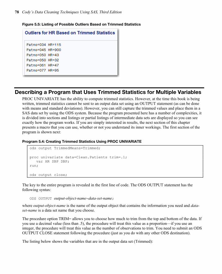
Figure 5.5: Listing of Possible Outliers Based on Trimmed Statistics

Describing a Program that Uses Trimmed Statistics for Multiple Variables PROC UNIVARIATE has the ability to compute trimmed statistics. However, at the time this book is being written, trimmed statistics cannot be sent to an output data set using an OUTPUT statement (as can be done with means and standard deviations). However, you can still capture the trimmed values and place them in a SAS data set by using the ODS system. Because the program presented here has a number of complexities, it is divided into sections and listings or partial listings of intermediate data sets are displayed so you can see exactly how the program works. If you are simply interested in results, the next section of this chapter presents a macro that you can use, whether or not you understand its inner workings. The first section of the program is shown next:

Program 5.4: Creating Trimmed Statistics Using PROC UNIVARIATE

ods output TrimmedMeans=Trimmed;

proc univariate data=Clean.Patients trim=.1; var HR SBP DBP; run;

ods output close;

The key to the entire program is revealed in the first line of code. The ODS OUTPUT statement has the following syntax:

ODS OUTPUT output-object-name=data-set-name;

where output-object-name is the name of the output object that contains the information you need and data-set-name is a data set name that you choose.

The procedure option TRIM= allows you to choose how much to trim from the top and bottom of the data. If you use a decimal value (less than .5), the procedure will treat this value as a proportion—if you use an integer, the procedure will treat this value as the number of observations to trim. You need to submit an ODS OUTPUT CLOSE statement following the procedure (just as you do with any other ODS destination).

The listing below shows the variables that are in the output data set (Trimmed):


Figure 5.6: Listing of Data Set Trimmed

The variables you want are the Mean (this is a trimmed mean), the StdMean, and the DF. What you really want is the trimmed standard deviation. However, this data set contains what is called the standard error instead. You can compute a standard deviation from a standard error by multiplying the standard error by the square root of the sample size, n. But you don't have n in the data set. No worries. The degrees of freedom (abbreviated DF) is equal to n – 1. Therefore, n is equal to DF + 1. By the way, the standard error reported by PROC UNIVARIATE is already adjusted for the amount of trimming you request.

The next problem you need to tackle is to restructure data set Patients so that you can merge it with data set Trimmed. Thus, the next block of code creates a separate observation for each patient and measure (HR, SBP, and DBP):


data Restructure; set Clean.Patients; length VarName $ 32; array Vars[*] HR SBP DBP; do i = 1 to dim(Vars); VarName = vname(Vars[i]); Value = Vars[i]; output; end; keep Patno VarName Value; run;

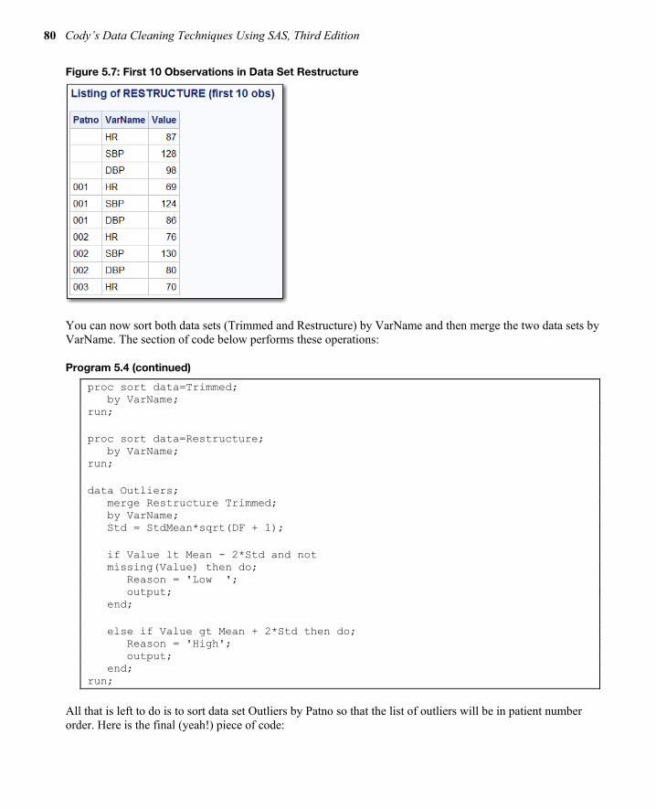
This section of code restructures the Patients data set so that it shares the variable VarName with data set Trimmed, thus allowing you to merge the two data sets using VarName as the BY variable. One of the keys to this section of code is the VNAME function. This function takes an array element as its argument and returns the variable name associated with this array element. Here is a listing of the first 10 observations in data set Restructure:


Figure 5.7: First 10 Observations in Data Set Restructure

You can now sort both data sets (Trimmed and Restructure) by VarName and then merge the two data sets by VarName. The section of code below performs these operations:


proc sort data=Trimmed; by VarName; run;

proc sort data=Restructure; by VarName; run;

data Outliers; merge Restructure Trimmed; by VarName; Std = StdMean*sqrt(DF + 1);

if Value lt Mean - 2*Std and not missing(Value) then do; Reason = 'Low '; output; end;

else if Value gt Mean + 2*Std then do; Reason = 'High'; output; end; run;

All that is left to do is to sort data set Outliers by Patno so that the list of outliers will be in patient number order. Here is the final (yeah!) piece of code:



proc sort data=Outliers; by Patno; run;

title "Outliers based on trimmed Statistics"; proc print data=outliers; id patno; var Varname Value Reason; run;

Here is a partial listing of the final report:

Figure 5.8: Partial Listing of Data Set Outliers

This listing is based on trimmed statistics (10% trim) and a cutoff of two standard deviations. The next section presents a macro based on this program. This macro allows you to select the amount to trim and the number of standard deviations for the cutoff.

Presenting a Macro Based on Trimmed Statistics This macro is presented without extensive explanation, mostly because it is based on Program 5.4, which was described in detail. Here is the listing:


Program 5.5: Presenting a Macro Based on Trimmed Statistics

*Method using automatic outlier detection; %macro Auto_Outliers( Dsn=, /* Data set name */ ID=, /* Name of ID variable */ Var_list=, /* List of variables to check */ /* separate names with spaces */ Trim=.1, /* Integer 0 to n = number to trim */ /* from each tail; if between 0 and .5, */ /* proportion to trim in each tail */ N_sd=2 /* Number of standard deviations */);

ods listing close; ods output TrimmedMeans=Trimmed(keep=VarName Mean Stdmean DF); proc univariate data=&Dsn trim=&Trim; var &Var_list; run; ods output close;

data Restructure; set &Dsn; length VarName $ 32; array Vars[*] &Var_list; do i = 1 to dim(Vars); VarName = vname(Vars[i]); Value = Vars[i]; output; end; keep &ID VarName Value; run;

proc sort data=Trimmed; by VarName; run;

proc sort data=restructure; by VarName; run; data Outliers; merge Restructure Trimmed; by VarName; Std = StdMean*sqrt(DF + 1); if Value lt Mean - &N_sd*Std and not missing(Value) then do; Reason = 'Low '; output; end; else if Value gt Mean + &N_sd*Std then do; Reason = 'High'; output; end; run;


proc sort data=Outliers; by &ID; run;

ods listing; title "Outliers Based on Trimmed Statistics"; proc print data=Outliers; id &ID; var VarName Value Reason; run;

proc datasets nolist library=work; delete Trimmed; delete Restructure; run; quit; %mend Auto_Outliers;

One feature of the macro is that values for Trim (.1) and the number of standard deviations (2) are set as default values. You may ask, "How much should I trim my data?" If you believe that your data set is pretty clean, you might choose a small trim value such as .05 or .1. For data that could contain many errors or where the distributions are heavily skewed, you might need to trim by .2 or even .25. Running this macro as follows results in the same output as in Figure 5.8:

%Auto_Outliers(Dsn=Clean.Patients, Id=Patno, Var_List=HR SBP DBP, Trim=.1, N_Sd=2)

Detecting Outliers Based on the Interquartile Range Yet another way to look for outliers is a method devised by advocates of exploratory data analysis (EDA). This is a robust method, much like the previous method based on trimmed statistics. It uses the interquartile range (the distance from the 25th percentile to the 75th percentile) and defines an outlier as a multiple of the interquartile range above the 75th percentile or below the 25th percentile. For those not familiar with EDA terminology, the first quartile (Q1) is the value corresponding to the 25th percentile (the value below which 25% of the data values lie). The third quartile (Q3) is the value corresponding to the 75% percentile. For example, you might want to examine any data values more than 1.5 times the interquartile range above Q3 or 1.5 times the interquartile range below Q1 as outliers. This is an attractive method because it is independent of the distribution of the data values.

You can use PROC SGPLOT to display a box plot, a graphical display that uses EDA techniques. As an example, let's generate a box plot for SBP in the Patients data set:

Program 5.6: Using PROC SGPLOT to Create a Box Plot

*Using PROC SGPLOT to Create a Box Plot for SBP; title "Using PROC SGPLOT to Create a Box Plot"; proc sgplot data=clean.Patients(keep=Patno SBP); hbox SBP; run;


PROC SGPLOT can create many types of graphical displays such as bar charts, scatter plots, and box plots. To create a box plot, use the HBOX statement followed by the names of one or more variables that you want to display. Here is the output:

Figure 5.9: Box Plot for SBP

The vertical line in the center of the box is the median and the diamond inside the box represents the mean. The left side and the right side of the box represent the first and third quartiles, respectively. The lines extending from both sides of the box represent a distance of 1.5 times the interquartile range from the sides of the box. (These lines are sometimes referred to as whiskers and the box plot is sometimes called a box-and-whisker plot.) Finally, the circles represent possible outliers—data points more than 1.5 times the interquartile range below the first quartile or above the third quartile.

You can also use SGPLOT to display box plots at each level of a categorical variable. To demonstrate this, let's create a box plot of SBP for each level of Gender. Because there were a number of data errors for Gender, the program shown next restricts values of Gender to 'F' and 'M':

Program 5.7: Creating a Box Plot for SBP for Each Level of Gender

*Using PROC SGPLOT to Create a Box Plot for SBP; title "Using PROC SGPLOT to Create a Box Plot"; proc sgplot data=clean.Patients(keep=Patno SBP Gender where=(Gender in ('F','M'))); hbox SBP / category=Gender; run;

The output (below) displays a box plot for each value of Gender:



An easy way to determine the interquartile range and the first and third quartiles is to use PROC MEANS to output these quantities. The program below is similar to Program 5.1 except it uses a criterion based on the interquartile range instead of the standard deviation:

Program 5.8: Detecting Outliers Using the Interquartile Range

title "Outliers Based on Interquartile Range"; proc means data=Clean.Patients noprint; var HR; output out=Tmp Q1= Q3= QRange= / autoname; run;

data _null_; file print; set Clean.Patients(keep=Patno HR); if _n_ = 1 then set Tmp; if HR le HR_Q1 - 1.5*HR_QRange and not missing(HR) or HR ge HR_Q3 + 1.5*HR_QRange then put "Possible Outlier for patient " Patno "Value of HR is " HR; run;

The keywords Q1, Q3, and QRange refer to the first quartile, the third quartile, and the interquartile range, respectively. Here is the output:



You can adjust Program 5.8 to produce more or fewer possible outliers by changing the number of interquartile ranges from 1.5 to other values.

You might prefer using the interquartile range for heavily skewed data, but with sufficient trimming, you will probably see similar results with the Auto_Outliers macro.

Conclusions This chapter investigated techniques that use the distribution of data values to identify possible data errors. You saw that using an algorithm based on the standard deviation can fail if there are some extreme values in the data. Ways to overcome this problem included using trimmed statistics or methods based on the interquartile range. There are times when data distributions are sufficiently different from a normal distribution where even trimmed statistics will fail to identify data errors. There is still hope. The next chapter discusses techniques that can be used on highly skewed data sets.

From Cody's Data Cleaning Techniques Using SAS®, Third Edition by Ron Cody. Copyright © 2017, SAS Institute Inc., Cary, North Carolina, USA. ALL RIGHTS RESERVED.


About This Book

What Does This Book Cover? As the title implies, this is a book that shows you how to use SAS to identify (and fix) errors in your data. The book covers several different ways of detecting errors in character and numeric data.

There are several chapters devoted to checking character data, including simple DATA step programming, using formats to detect data errors, using Perl regular expressions to check that data values conform to a pre-determined pattern, and finally, standardizing such values as company names and addresses.

Checking for errors in numeric data is approached using several techniques. For some numeric values such as age or heart rate, you can use pre-determined ranges. For other types of numeric data, you can use techniques that automatically detect possible errors. This book also presents some statistical tests based on regression diagnostics that might find data errors when other methods fail.

This book includes a chapter describing several methods for correcting data errors and a chapter that describes SAS integrity constraints and audit trails. Briefly, integrity constraints are rules about your data that are stored inside a SAS data set that can block data errors when you add new data to an existing, previously cleaned data set.

Besides teaching you programming techniques, this book includes a collection of macros (pre-packaged SAS code) that you can use right out of the box or modify for your own particular task. Keep in mind that all of the programs, data, and macros in this book are available in a free download from the web site support.sas.com/cody.

Is This Book for You? Just about anyone who is in the business of analyzing data needs to check that data for errors before engaging in any type of analysis. This book will save you the trouble of reinventing the wheel and having to create all your data cleaning programs from scratch.

What Are the Prerequisites for This Book? This book assumes that you know some basic SAS programming skills. Those readers who are relatively new to SAS will appreciate the fact that all of the programs developed in the book are described in detail—those readers with more advanced programming skills will appreciate the innovative techniques developed to clean data.

http://support.sas.com/publishing/authors/cody.html

xvi

What’s New in This Edition? This book is a third edition. Many second and third editions reflect minor changes from the original. This one does not. It has been over 10 years since the author wrote the second edition, and lots of things have changed since then—both the experience gained from teaching a data cleaning course for those 10 years and advances in SAS. This third edition is a major upgrade from its sibling. One of the first things you will notice are four new chapters, covering topics such as the use of Perl regular expressions for checking the format of character values (such as ZIP codes or email addresses) and how to standardize company names and addresses. One of the new chapters describes how to identify possible data errors in highly skewed distributions using regression diagnostics.

What Should You Know about the Examples? Every program presented in this book is explained in detail, and you can run any of these programs yourself because they are all included in a free download of programs and data from the SAS author site.

Software Used to Develop the Book's Content Most of the programs in this book can be run using base SAS, using any SAS platform that you typically use to analyze your data. A few of the more advanced techniques for detecting errors in numeric data use procedures found in SAS/STAT software.

SAS University Edition

This book is compatible with SAS University Edition.

Output and Graphics All of the output from the programs presented in this book are displayed with explanations and, in some cases, annotations.

We Want to Hear from You SAS Press books are written by SAS users for SAS users. We welcome your participation in their development and your feedback on SAS Press books that you are using. Please visit https://support.sas.com/publishing to do the following:

● Sign up to review a book ● Recommend a topic ● Request information on how to become a SAS Press author ● Provide feedback on a book

Do you have questions about a SAS Press book that you are reading? Contact the author through [email protected] or https://support.sas.com/author_feedback.

SAS has many resources to help you find answers and expand your knowledge. If you need additional help, see our list of resources: https://support.sas.com/publishing.

https://support.sas.com/publishing

mailto:[email protected]

https://support.sas.com/author_feedback

https://support.sas.com/publishing

About The Author

Ron Cody, EdD, a retired professor from the Rutgers Robert Wood Johnson Medical School, now works as a private consultant and a national instructor for SAS Institute Inc. A SAS user since 1977, Ron's extensive knowledge and innovative style have made him a popular presenter at local, regional, and national SAS conferences. He has authored or co-authored numerous books, as well as countless articles in medical and scientific journals.

Learn more about this author by visiting his author page at http://support.sas.com/cody. There you can download free book excerpts, access example code and data, read the latest reviews, get updates, and more.

http://support.sas.com/cody

cody's data cleaning techniques using sas®, third edition · chapter 4: data cleaning...

Documents