Cluster Analysis: Basic Concepts and Algorithms

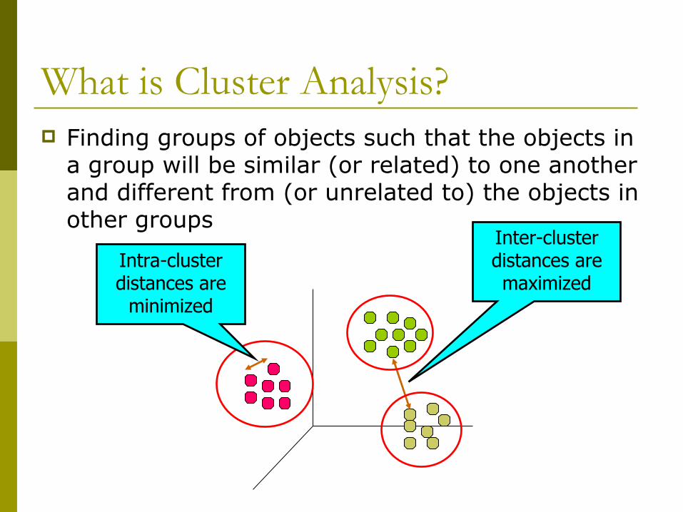
What is Cluster Analysis? Finding groups of objects such that the objects in

a group will be similar (or related) to one another and different from (or unrelated to) the objects in other groups

Inter-cluster distances are maximized

Intra-cluster distances are

minimized

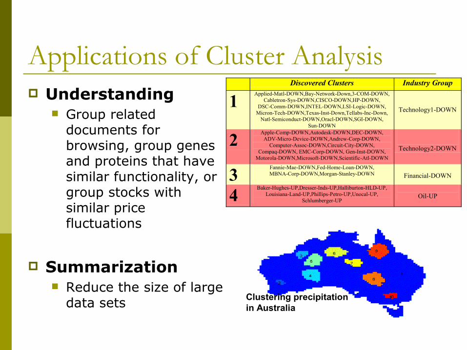
Applications of Cluster Analysis Understanding

Group related documents for browsing, group genes and proteins that have similar functionality, or group stocks with similar price fluctuations

Summarization Reduce the size of large

data sets

Discovered Clusters Industry Group

1 Applied-Matl-DOWN,Bay-Network-Down,3-COM-DOWN, Cabletron-Sys-DOWN,CISCO-DOWN,HP-DOWN,

DSC-Comm-DOWN,INTEL-DOWN,LSI-Logic-DOWN, Micron-Tech-DOWN,Texas-Inst-Down,Tellabs-Inc-Down,

Natl-Semiconduct-DOWN,Oracl-DOWN,SGI-DOWN, Sun-DOWN

Technology1-DOWN

2 Apple-Comp-DOWN,Autodesk-DOWN,DEC-DOWN, ADV-Micro-Device-DOWN,Andrew-Corp-DOWN,

Computer-Assoc-DOWN,Circuit-City-DOWN, Compaq-DOWN, EMC-Corp-DOWN, Gen-Inst-DOWN,

Motorola-DOWN,Microsoft-DOWN,Scientific-Atl-DOWN

Technology2-DOWN

3 Fannie-Mae-DOWN,Fed-Home-Loan-DOWN, MBNA-Corp-DOWN,Morgan-Stanley-DOWN

Financial-DOWN

4 Baker-Hughes-UP,Dresser-Inds-UP,Halliburton-HLD-UP, Louisiana-Land-UP,Phillips-Petro-UP,Unocal-UP,

Schlumberger-UP

Oil-UP

Clustering precipitation in Australia

Notion of a Cluster can be Ambiguous

How many clusters?

Four Clusters Two Clusters

Six Clusters

Types of Clusterings A clustering is a set of clusters

Important distinction between hierarchical and partitional sets of clusters

Partitional Clustering A division data objects into non-overlapping subsets

(clusters) such that each data object is in exactly one subset

Hierarchical clustering A set of nested clusters organized as a hierarchical

tree

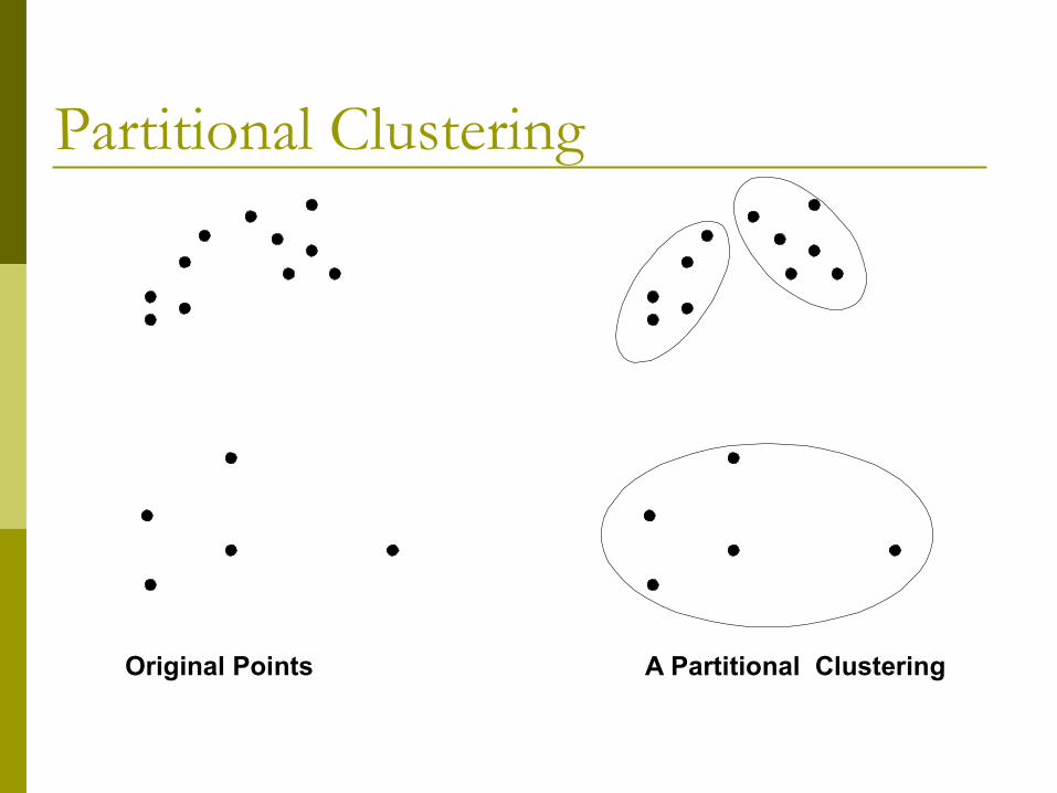
Partitional Clustering

Original Points A Partitional Clustering

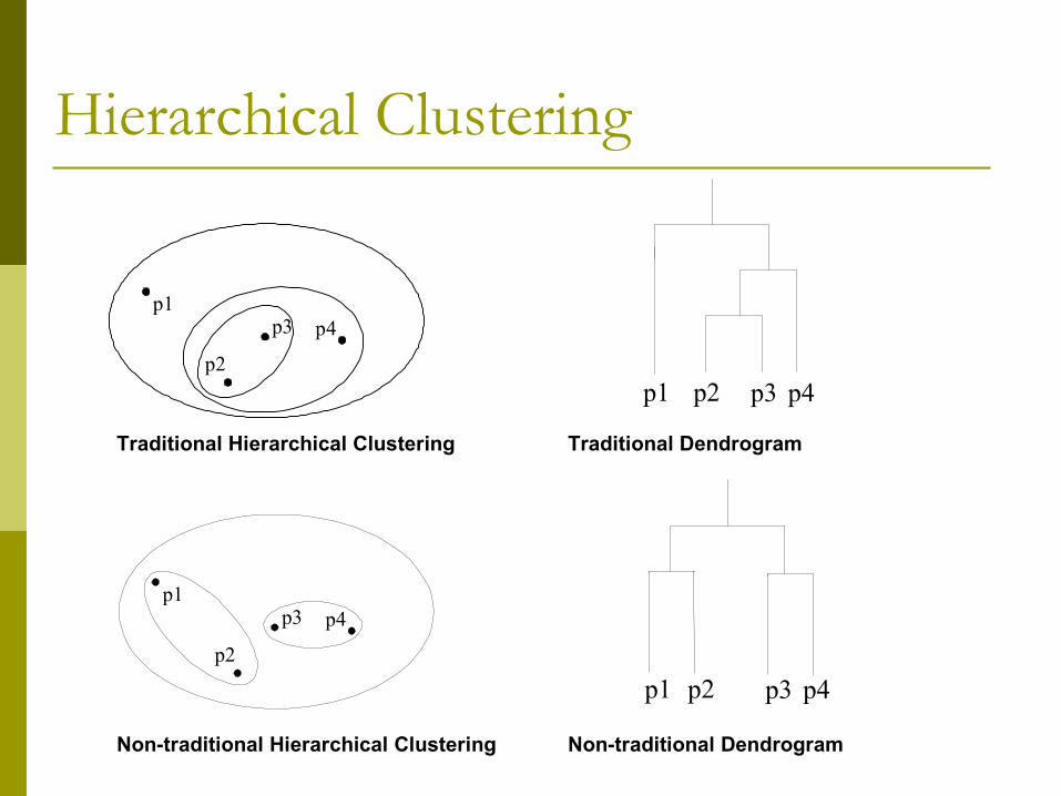
Hierarchical Clustering

p4p1

p3

p2

p4 p1

p3

p2 p4p1 p2 p3

p4p1 p2 p3

Traditional Hierarchical Clustering

Non-traditional Hierarchical Clustering Non-traditional Dendrogram

Traditional Dendrogram

Other Distinctions Between Sets of Clusters

Exclusive versus non-exclusive In non-exclusive clusterings, points may belong to

multiple clusters. Can represent multiple classes or ‘border’ points

Fuzzy versus non-fuzzy In fuzzy clustering, a point belongs to every cluster

with some weight between 0 and 1 Weights must sum to 1 Probabilistic clustering has similar characteristics

Partial versus complete In some cases, we only want to cluster some of the

data Heterogeneous versus homogeneous

Cluster of widely different sizes, shapes, and densities

Clustering Algorithms K-means and its variants

Hierarchical clustering

Density-based clustering

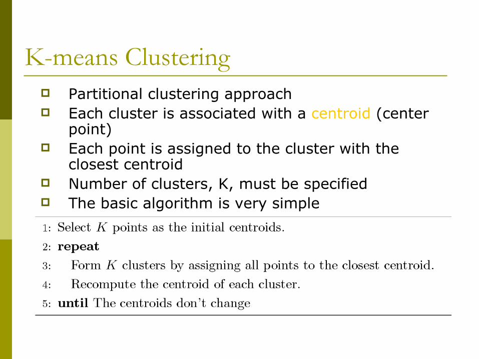
K-means Clustering Partitional clustering approach Each cluster is associated with a centroid (center

point) Each point is assigned to the cluster with the

closest centroid Number of clusters, K, must be specified The basic algorithm is very simple

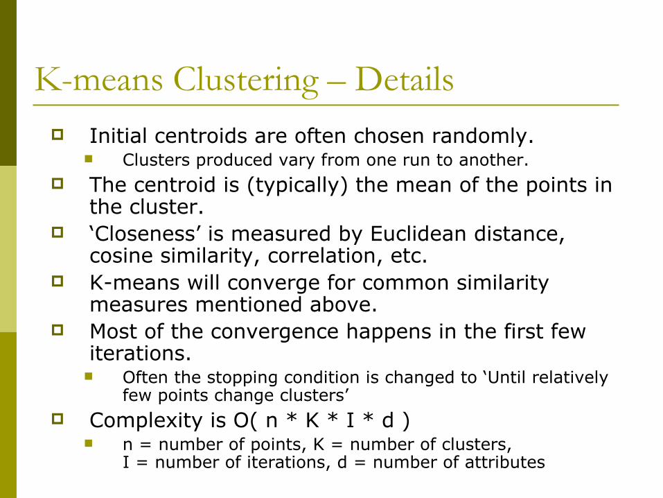
K-means Clustering – Details Initial centroids are often chosen randomly.

Clusters produced vary from one run to another. The centroid is (typically) the mean of the points in

the cluster. ‘Closeness’ is measured by Euclidean distance,

cosine similarity, correlation, etc. K-means will converge for common similarity

measures mentioned above. Most of the convergence happens in the first few

iterations. Often the stopping condition is changed to ‘Until relatively

few points change clusters’ Complexity is O( n * K * I * d )

n = number of points, K = number of clusters, I = number of iterations, d = number of attributes

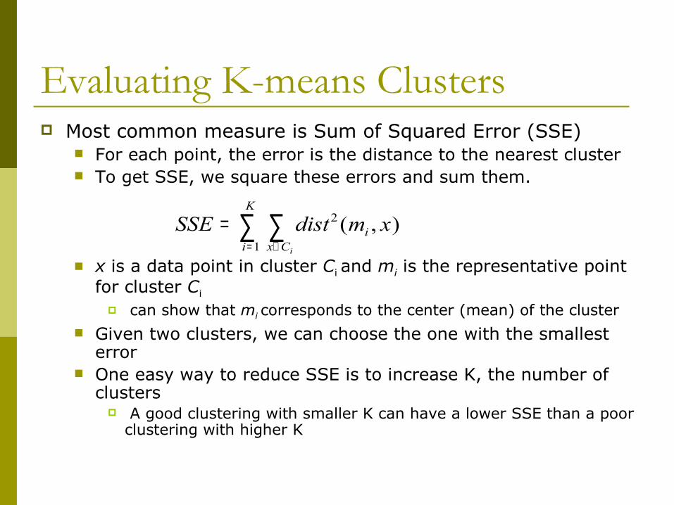
Evaluating K-means Clusters Most common measure is Sum of Squared Error (SSE)

For each point, the error is the distance to the nearest cluster To get SSE, we square these errors and sum them.

x is a data point in cluster Ci and mi is the representative point for cluster Ci

can show that mi corresponds to the center (mean) of the cluster Given two clusters, we can choose the one with the smallest

error One easy way to reduce SSE is to increase K, the number of

clusters A good clustering with smaller K can have a lower SSE than a poor

clustering with higher K

∑ ∑= ∈

=K

i Cxi

i

xmdistSSE1

2 ),(

Issues and Limitations for K-means How to choose initial centers? How to choose K? How to handle Outliers? Clusters different in

Shape Density Size

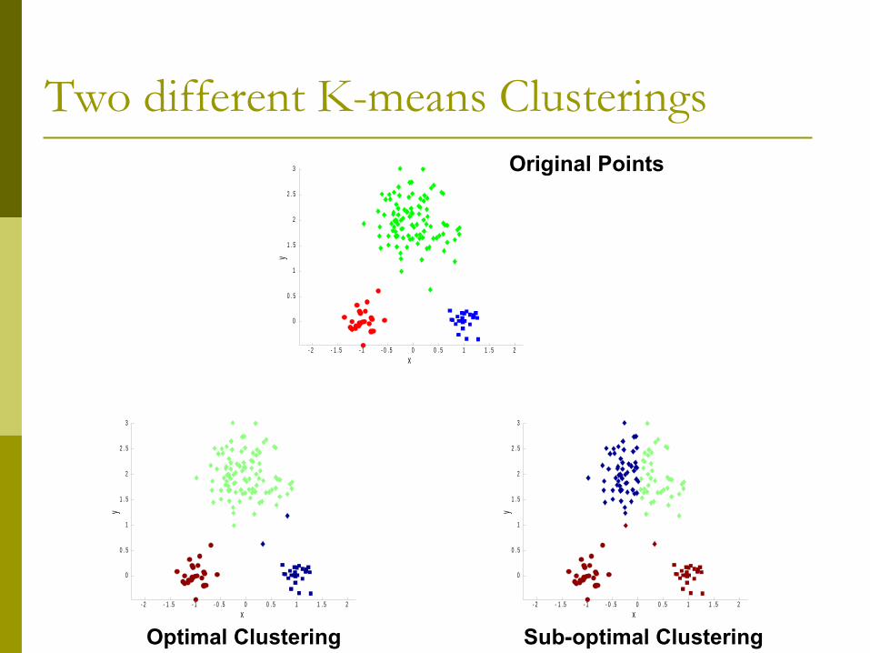
Two different K-means Clusterings

- 2 - 1 .5 - 1 - 0 .5 0 0 . 5 1 1 . 5 2

0

0 . 5

1

1 . 5

2

2 . 5

3

x

y

- 2 - 1 .5 - 1 - 0 .5 0 0 . 5 1 1 . 5 2

0

0 . 5

1

1 . 5

2

2 . 5

3

x

y

Sub-optimal Clustering- 2 - 1 .5 - 1 - 0 .5 0 0 . 5 1 1 . 5 2

0

0 . 5

1

1 . 5

2

2 . 5

3

x

y

Optimal Clustering

Original Points

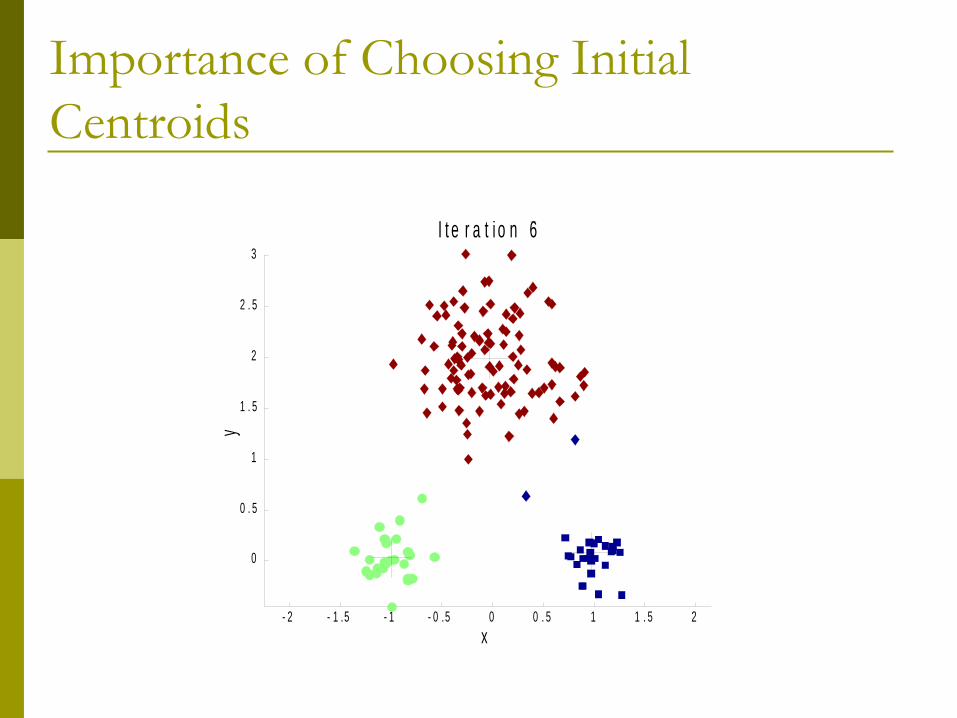
Importance of Choosing Initial Centroids

- 2 - 1 .5 - 1 - 0 .5 0 0 . 5 1 1 . 5 2

0

0 . 5

1

1 . 5

2

2 . 5

3

x

yI t e r a t i o n 1

- 2 - 1 .5 - 1 - 0 .5 0 0 . 5 1 1 . 5 2

0

0 . 5

1

1 . 5

2

2 . 5

3

x

yI t e r a t i o n 2

- 2 - 1 .5 - 1 - 0 .5 0 0 . 5 1 1 . 5 2

0

0 . 5

1

1 . 5

2

2 . 5

3

x

yI t e r a t i o n 3

- 2 - 1 .5 - 1 - 0 .5 0 0 . 5 1 1 . 5 2

0

0 . 5

1

1 . 5

2

2 . 5

3

x

yI t e r a t i o n 4

- 2 - 1 .5 - 1 - 0 .5 0 0 . 5 1 1 . 5 2

0

0 . 5

1

1 . 5

2

2 . 5

3

x

yI t e r a t i o n 5

- 2 - 1 .5 - 1 - 0 .5 0 0 . 5 1 1 . 5 2

0

0 . 5

1

1 . 5

2

2 . 5

3

x

yI t e r a t i o n 6

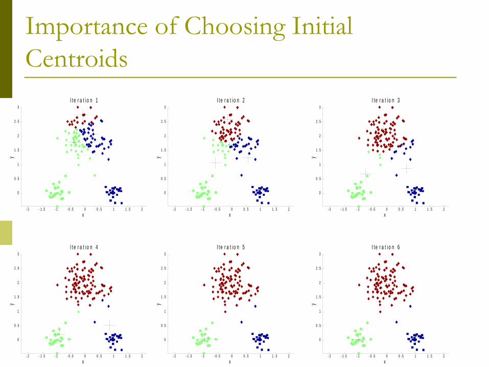
Importance of Choosing Initial Centroids

- 2 - 1 .5 - 1 - 0 .5 0 0 . 5 1 1 . 5 2

0

0 . 5

1

1 . 5

2

2 . 5

3

x

y

I t e r a t i o n 1

- 2 - 1 .5 - 1 - 0 .5 0 0 . 5 1 1 . 5 2

0

0 . 5

1

1 . 5

2

2 . 5

3

x

y

I t e r a t i o n 2

- 2 - 1 .5 - 1 - 0 .5 0 0 . 5 1 1 . 5 2

0

0 . 5

1

1 . 5

2

2 . 5

3

x

y

I t e r a t i o n 3

- 2 - 1 .5 - 1 - 0 .5 0 0 . 5 1 1 . 5 2

0

0 . 5

1

1 . 5

2

2 . 5

3

x

y

I t e r a t i o n 4

- 2 - 1 .5 - 1 - 0 .5 0 0 . 5 1 1 . 5 2

0

0 . 5

1

1 . 5

2

2 . 5

3

x

y

I t e r a t i o n 5

- 2 - 1 .5 - 1 - 0 .5 0 0 . 5 1 1 . 5 2

0

0 . 5

1

1 . 5

2

2 . 5

3

x

y

I t e r a t i o n 6

Importance of Choosing Initial Centroids …

- 2 - 1 .5 - 1 - 0 .5 0 0 . 5 1 1 . 5 2

0

0 . 5

1

1 . 5

2

2 . 5

3

x

yI t e r a t i o n 1

- 2 - 1 .5 - 1 - 0 .5 0 0 . 5 1 1 . 5 2

0

0 . 5

1

1 . 5

2

2 . 5

3

x

yI t e r a t i o n 2

- 2 - 1 .5 - 1 - 0 .5 0 0 . 5 1 1 . 5 2

0

0 . 5

1

1 . 5

2

2 . 5

3

x

yI t e r a t i o n 3

- 2 - 1 .5 - 1 - 0 .5 0 0 . 5 1 1 . 5 2

0

0 . 5

1

1 . 5

2

2 . 5

3

x

yI t e r a t i o n 4

- 2 - 1 .5 - 1 - 0 .5 0 0 . 5 1 1 . 5 2

0

0 . 5

1

1 . 5

2

2 . 5

3

x

yI t e r a t i o n 5

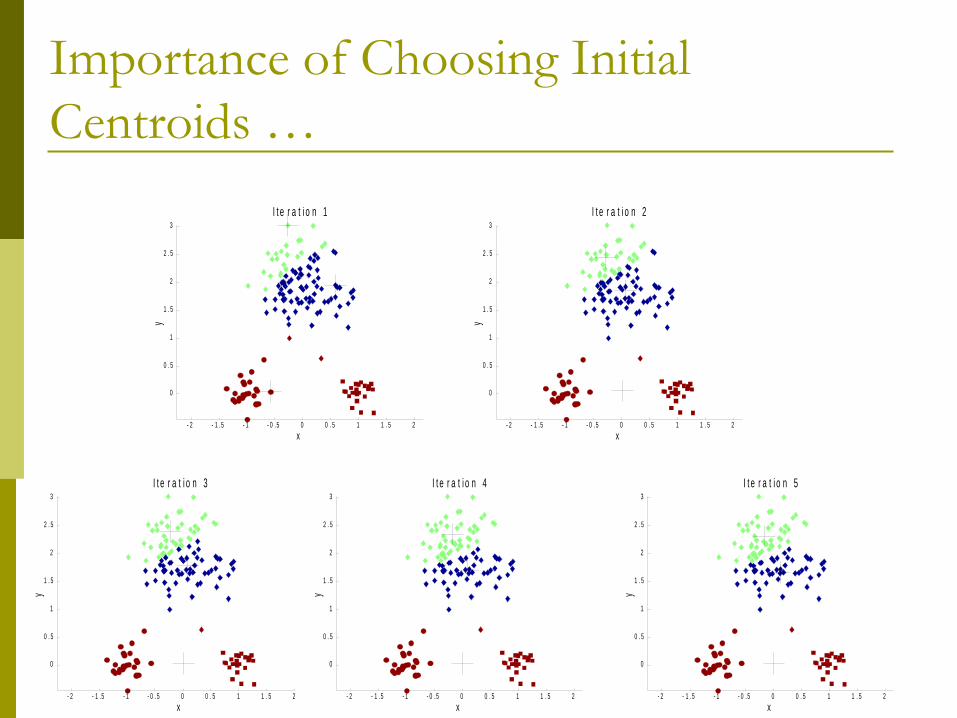
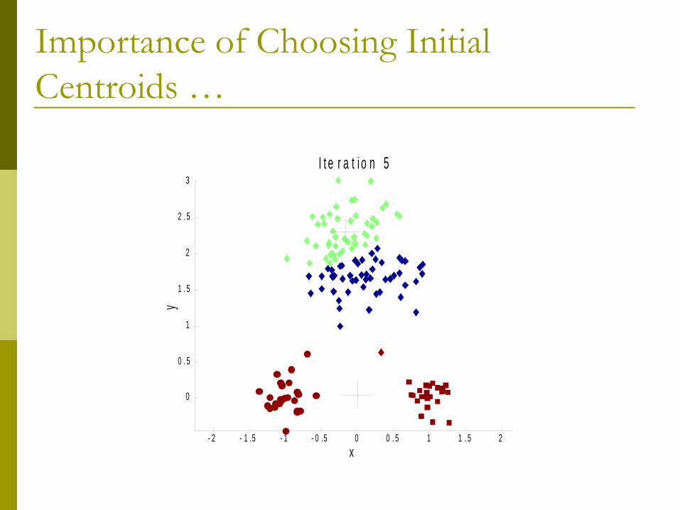
Importance of Choosing Initial Centroids …

- 2 - 1 .5 - 1 - 0 .5 0 0 . 5 1 1 . 5 2

0

0 . 5

1

1 . 5

2

2 . 5

3

x

y

I t e r a t i o n 1

- 2 - 1 .5 - 1 - 0 .5 0 0 . 5 1 1 . 5 2

0

0 . 5

1

1 . 5

2

2 . 5

3

x

y

I t e r a t i o n 2

- 2 - 1 .5 - 1 - 0 .5 0 0 . 5 1 1 . 5 2

0

0 . 5

1

1 . 5

2

2 . 5

3

x

y

I t e r a t i o n 3

- 2 - 1 .5 - 1 - 0 .5 0 0 . 5 1 1 . 5 2

0

0 . 5

1

1 . 5

2

2 . 5

3

x

y

I t e r a t i o n 4

- 2 - 1 .5 - 1 - 0 .5 0 0 . 5 1 1 . 5 2

0

0 . 5

1

1 . 5

2

2 . 5

3

x

y

I t e r a t i o n 5

Problems with Selecting Initial Points

If there are K ‘real’ clusters then the chance of selecting one centroid from each cluster is small. Chance is relatively small when K is large If clusters are the same size, n, then

For example, if K = 10, then probability = 10!/1010 = 0.00036

Sometimes the initial centroids will readjust themselves in ‘right’ way, and sometimes they don’t

Consider an example of five pairs of clusters

Solutions to Initial Centroids Problem Multiple runs

Helps, but probability is not on your side Sample and use hierarchical clustering to

determine initial centroids Select more than k initial centroids and

then select among these initial centroids Select most widely separated

Postprocessing Bisecting K-means

Not as susceptible to initialization issues

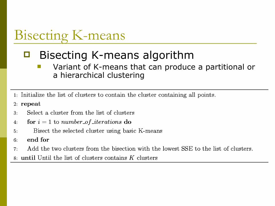
Bisecting K-means Bisecting K-means algorithm

Variant of K-means that can produce a partitional or a hierarchical clustering

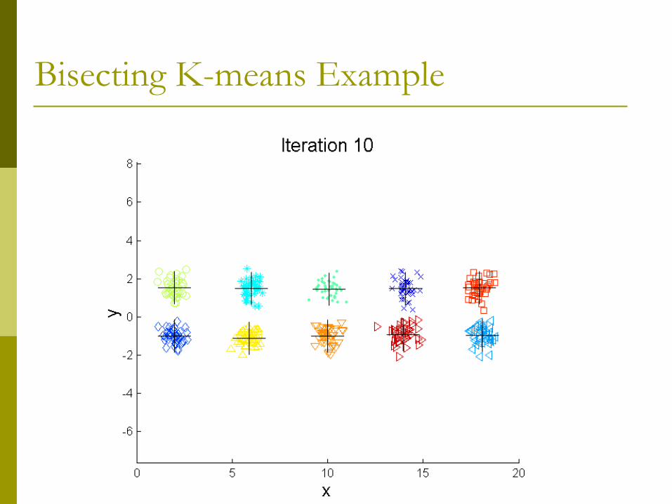
Bisecting K-means Example

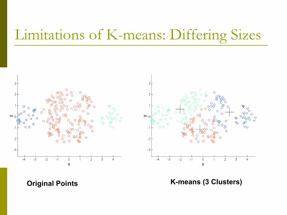
Limitations of K-means: Differing Sizes

Original Points K-means (3 Clusters)

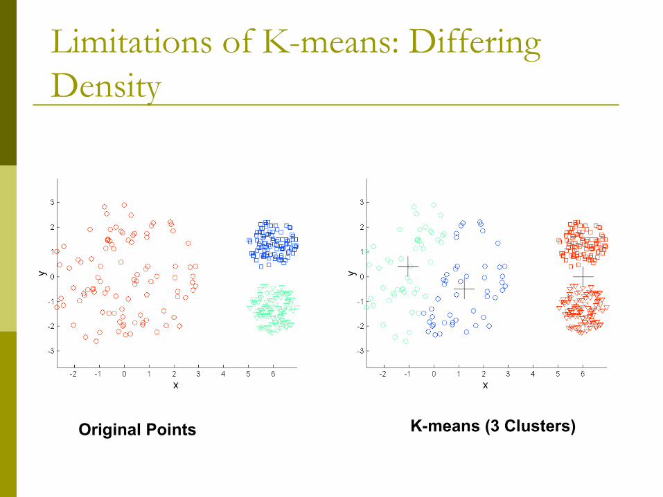
Limitations of K-means: Differing Density

Original Points K-means (3 Clusters)

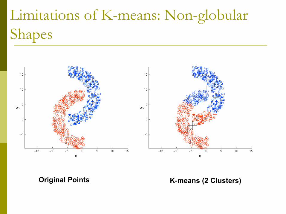
Limitations of K-means: Non-globular Shapes

Original Points K-means (2 Clusters)

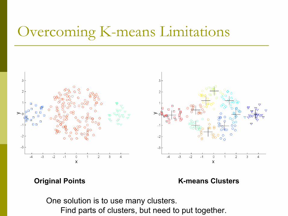
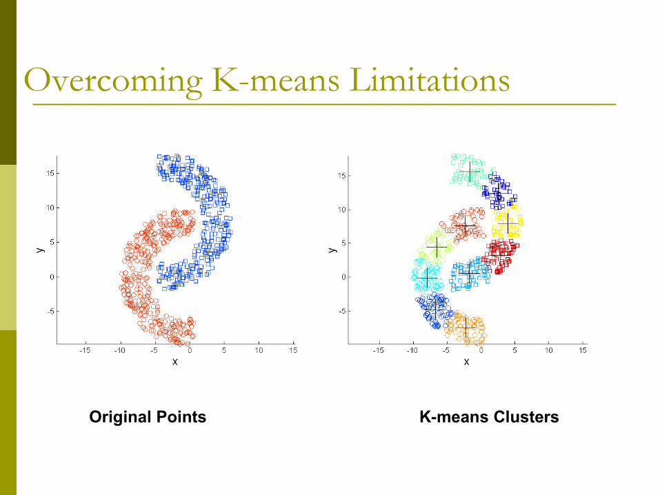
Overcoming K-means Limitations

Original Points K-means Clusters

One solution is to use many clusters.Find parts of clusters, but need to put together.

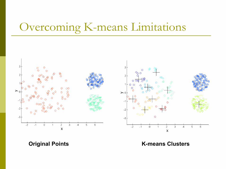
Overcoming K-means Limitations

Original Points K-means Clusters

Overcoming K-means Limitations

Original Points K-means Clusters

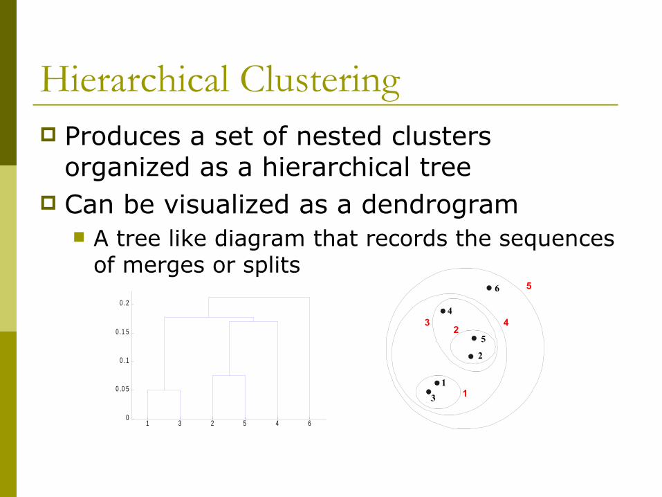
Hierarchical Clustering Produces a set of nested clusters

organized as a hierarchical tree Can be visualized as a dendrogram

A tree like diagram that records the sequences of merges or splits

1 3 2 5 4 60

0 .0 5

0 .1

0 .1 5

0 .2

1

2

3

4

5

6

1

23 4

5

Strengths of Hierarchical Clustering Do not have to assume any particular

number of clusters Any desired number of clusters can be

obtained by ‘cutting’ the dendogram at the proper level

They may correspond to meaningful taxonomies Example in biological sciences (e.g., animal

kingdom, phylogeny reconstruction, …)

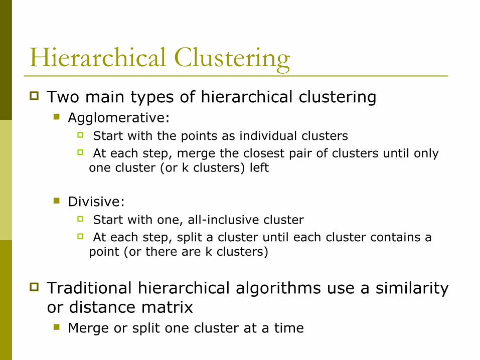
Hierarchical Clustering Two main types of hierarchical clustering

Agglomerative: Start with the points as individual clusters At each step, merge the closest pair of clusters until only

one cluster (or k clusters) left

Divisive: Start with one, all-inclusive cluster At each step, split a cluster until each cluster contains a

point (or there are k clusters)

Traditional hierarchical algorithms use a similarity or distance matrix Merge or split one cluster at a time

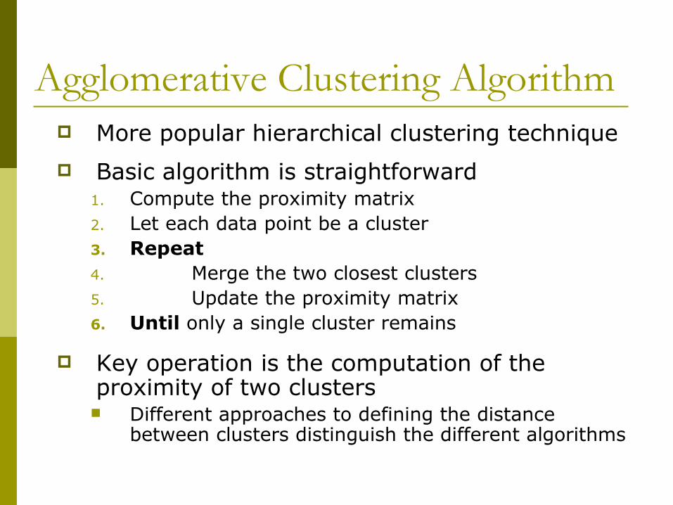
Agglomerative Clustering Algorithm More popular hierarchical clustering technique

Basic algorithm is straightforward1. Compute the proximity matrix2. Let each data point be a cluster3. Repeat4. Merge the two closest clusters5. Update the proximity matrix6. Until only a single cluster remains

Key operation is the computation of the proximity of two clusters Different approaches to defining the distance

between clusters distinguish the different algorithms

Starting Situation Start with clusters of individual points and

a proximity matrixp1

p3

p5

p4

p2

p1 p2 p3 p4 p5 . . .

.

.

. Proximity Matrix

...p1 p2 p3 p4 p9 p10 p11 p12

Intermediate Situation After some merging steps, we have some clusters

C1

C4

C2 C5

C3

C2C1

C1

C3

C5

C4

C2

C3 C4 C5

Proximity Matrix

...p1 p2 p3 p4 p9 p10 p11 p12

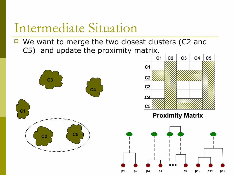
Intermediate Situation We want to merge the two closest clusters (C2 and

C5) and update the proximity matrix.

C1

C4

C2 C5

C3

C2C1

C1

C3

C5

C4

C2

C3 C4 C5

Proximity Matrix

...p1 p2 p3 p4 p9 p10 p11 p12

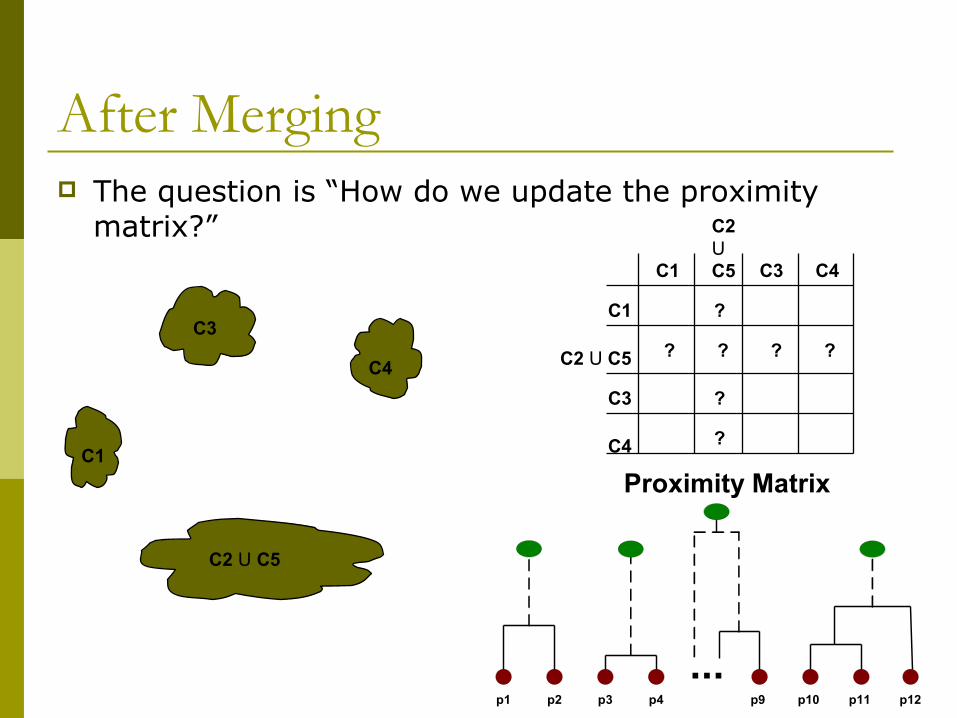
After Merging The question is “How do we update the proximity

matrix?”

C1

C4

C2 U C5

C3? ? ? ?

?

?

?

C2 U C5C1

C1

C3

C4

C2 U C5

C3 C4

Proximity Matrix

...p1 p2 p3 p4 p9 p10 p11 p12

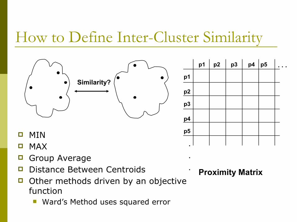
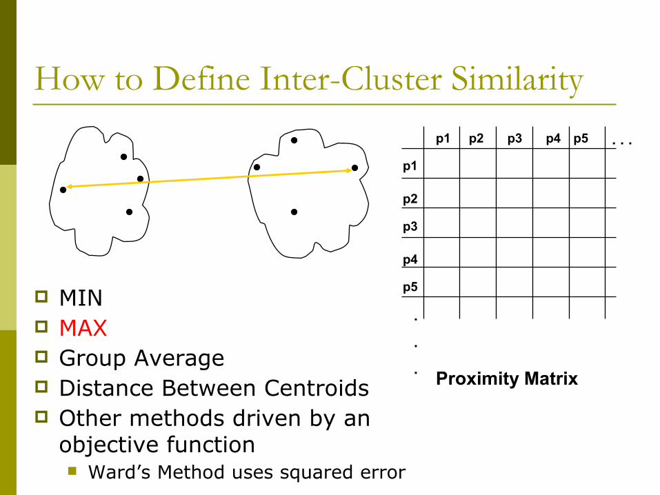
How to Define Inter-Cluster Similarity

p1

p3

p5

p4

p2

p1 p2 p3 p4 p5 . . .

.

.

.

Similarity?

MIN MAX Group Average Distance Between Centroids Other methods driven by an objective

function Ward’s Method uses squared error

Proximity Matrix

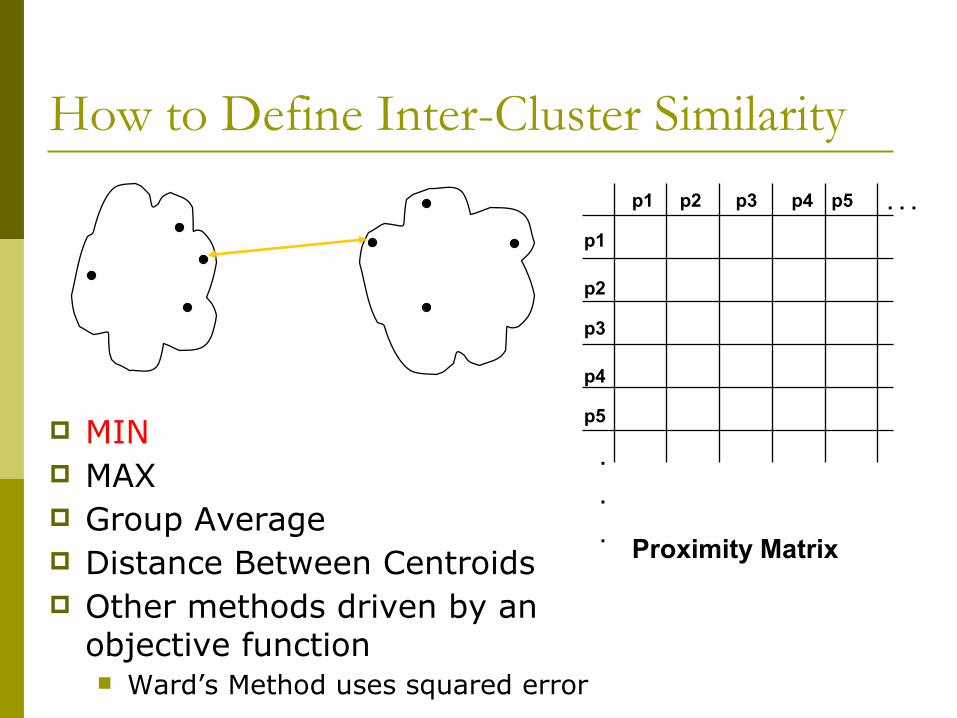
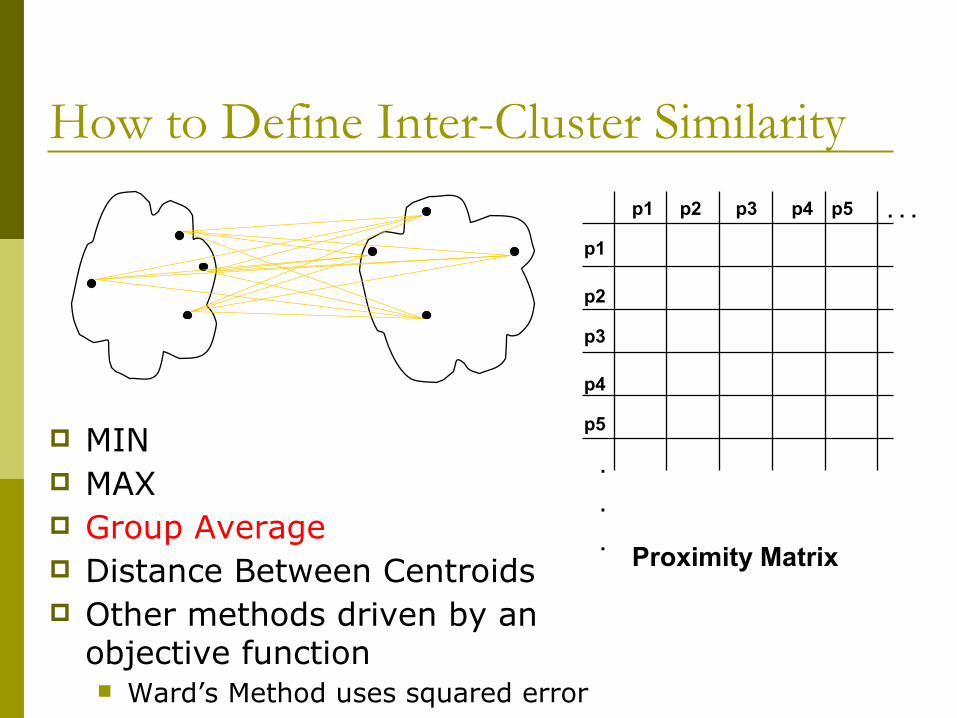
How to Define Inter-Cluster Similarity

p1

p3

p5

p4

p2

p1 p2 p3 p4 p5 . . .

.

.

. Proximity Matrix

MIN MAX Group Average Distance Between Centroids Other methods driven by an

objective function Ward’s Method uses squared error

How to Define Inter-Cluster Similarity

p1

p3

p5

p4

p2

p1 p2 p3 p4 p5 . . .

.

.

. Proximity Matrix

MIN MAX Group Average Distance Between Centroids Other methods driven by an

objective function Ward’s Method uses squared error

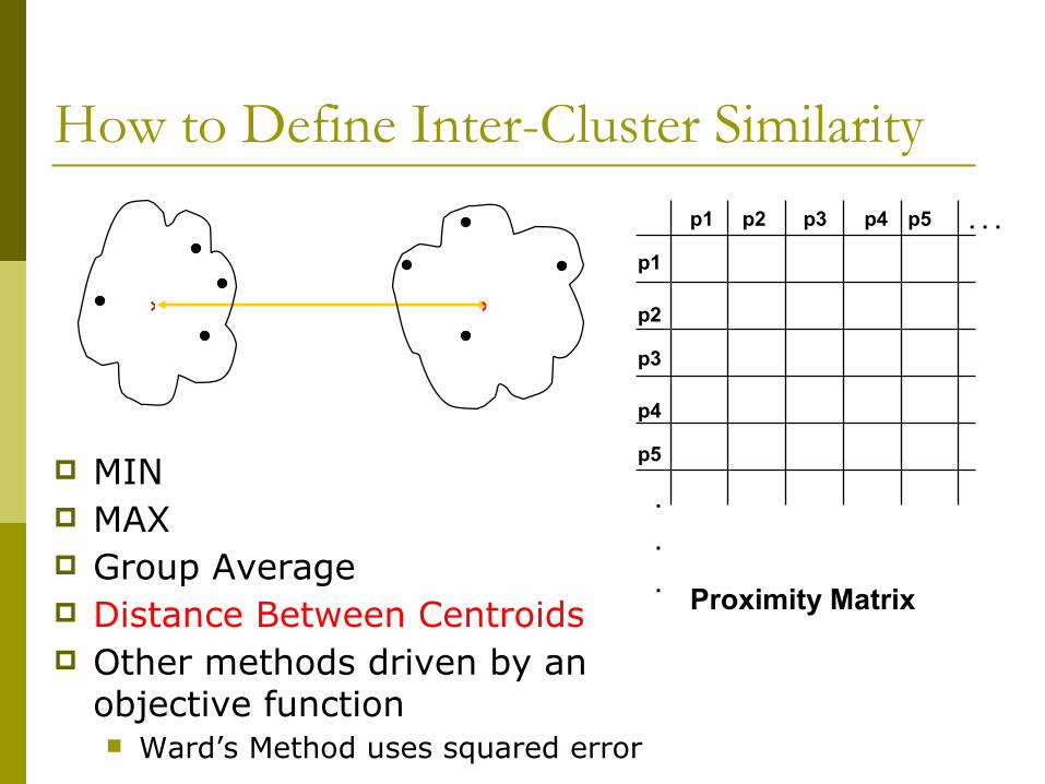
How to Define Inter-Cluster Similarity

p1

p3

p5

p4

p2

p1 p2 p3 p4 p5 . . .

.

.

. Proximity Matrix

MIN MAX Group Average Distance Between Centroids Other methods driven by an

objective function Ward’s Method uses squared error

How to Define Inter-Cluster Similarity

p1

p3

p5

p4

p2

p1 p2 p3 p4 p5 . . .

.

.

. Proximity Matrix

MIN MAX Group Average Distance Between Centroids Other methods driven by an

objective function Ward’s Method uses squared error

× ×

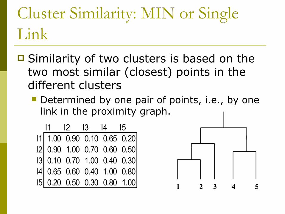
Cluster Similarity: MIN or Single Link Similarity of two clusters is based on the

two most similar (closest) points in the different clusters Determined by one pair of points, i.e., by one

link in the proximity graph.

I1 I2 I3 I4 I5I1 1.00 0.90 0.10 0.65 0.20I2 0.90 1.00 0.70 0.60 0.50I3 0.10 0.70 1.00 0.40 0.30I4 0.65 0.60 0.40 1.00 0.80I5 0.20 0.50 0.30 0.80 1.00 1 2 3 4 5

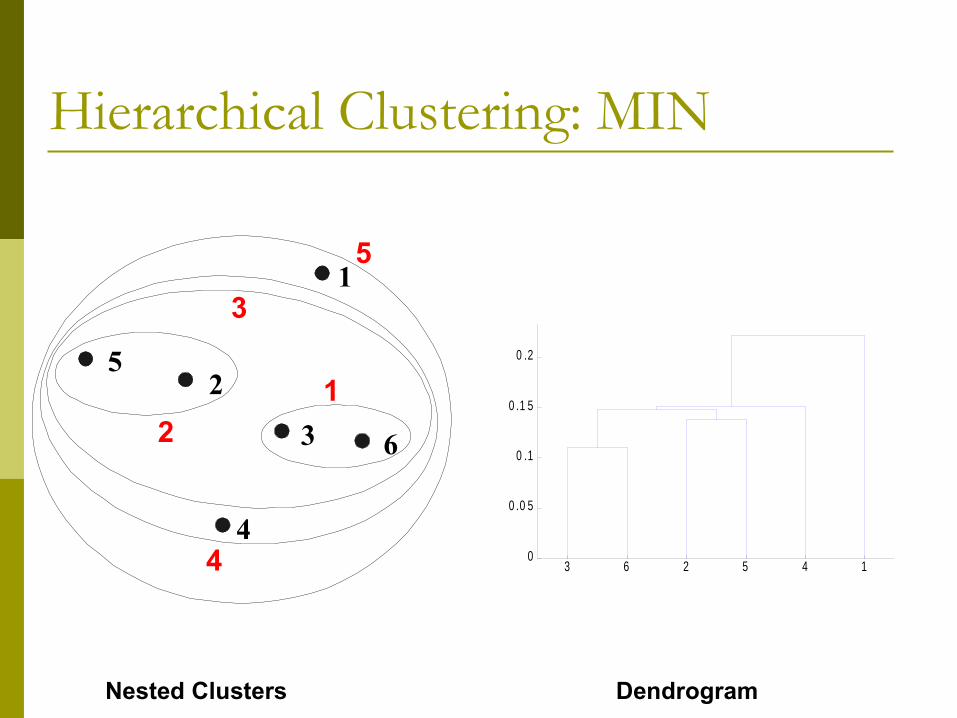
Hierarchical Clustering: MIN

Nested Clusters Dendrogram

1

2

3

4

5

6

12

3

4

5

3 6 2 5 4 10

0 .0 5

0 .1

0 .1 5

0 .2

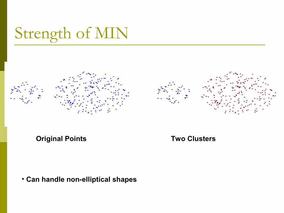
Strength of MIN

Original Points Two Clusters

• Can handle non-elliptical shapes

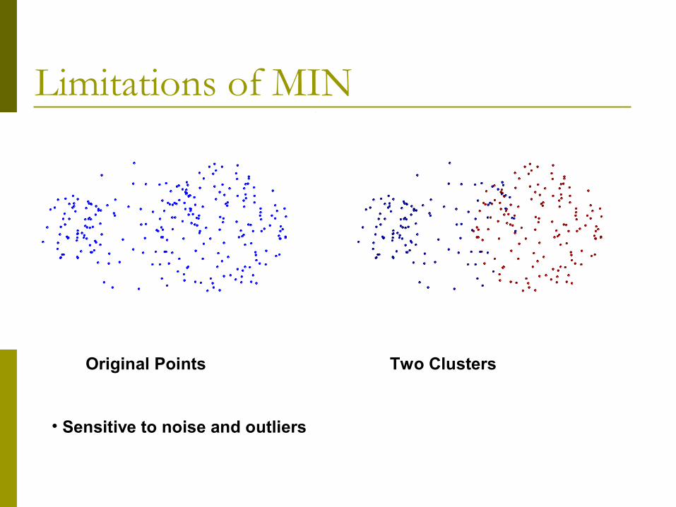
Limitations of MIN

Original Points Two Clusters

• Sensitive to noise and outliers

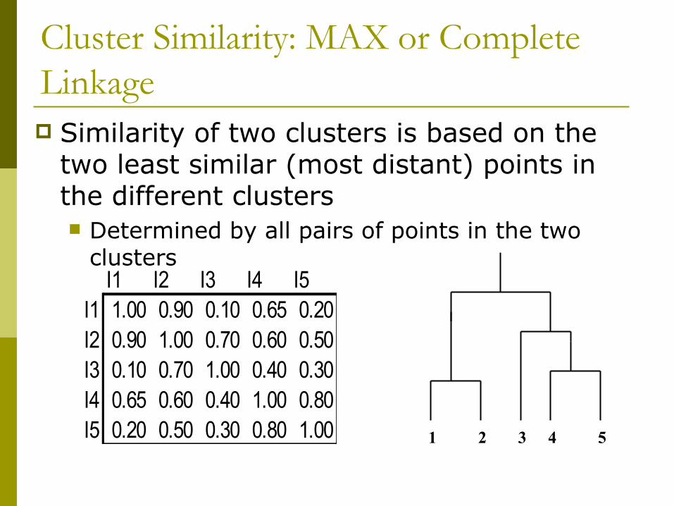
Cluster Similarity: MAX or Complete Linkage Similarity of two clusters is based on the

two least similar (most distant) points in the different clusters Determined by all pairs of points in the two

clustersI1 I2 I3 I4 I5

I1 1.00 0.90 0.10 0.65 0.20I2 0.90 1.00 0.70 0.60 0.50I3 0.10 0.70 1.00 0.40 0.30I4 0.65 0.60 0.40 1.00 0.80I5 0.20 0.50 0.30 0.80 1.00 1 2 3 4 5

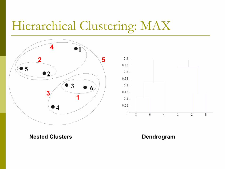
Hierarchical Clustering: MAX

Nested Clusters Dendrogram

3 6 4 1 2 50

0 .0 5

0 .1

0 .1 5

0 .2

0 .2 5

0 .3

0 .3 5

0 .4

1

2

3

4

5

61

2 5

3

4

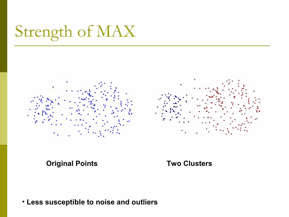
Strength of MAX

Original Points Two Clusters

• Less susceptible to noise and outliers

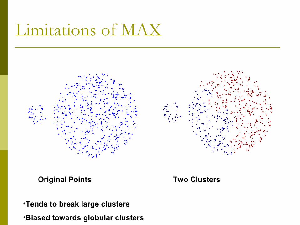
Limitations of MAX

Original Points Two Clusters

•Tends to break large clusters

•Biased towards globular clusters

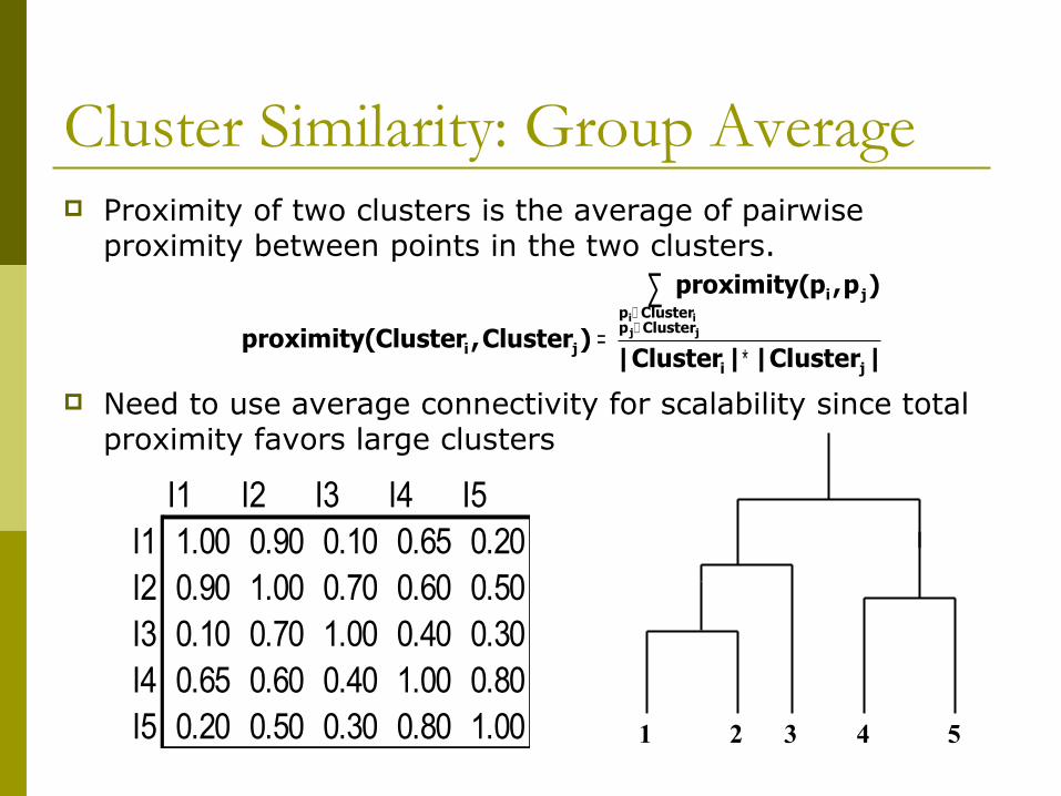
Cluster Similarity: Group Average Proximity of two clusters is the average of pairwise

proximity between points in the two clusters.

Need to use average connectivity for scalability since total proximity favors large clusters

||Cluster||Cluster

)p,pproximity(

)Cluster,Clusterproximity(ji

ClusterpClusterp

ji

jijjii

∗=

∑∈∈

I1 I2 I3 I4 I5I1 1.00 0.90 0.10 0.65 0.20I2 0.90 1.00 0.70 0.60 0.50I3 0.10 0.70 1.00 0.40 0.30I4 0.65 0.60 0.40 1.00 0.80I5 0.20 0.50 0.30 0.80 1.00 1 2 3 4 5

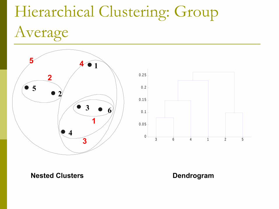
Hierarchical Clustering: Group Average

Nested Clusters Dendrogram

3 6 4 1 2 50

0 .0 5

0 .1

0 .1 5

0 .2

0 .2 5

1

2

3

4

5

61

2

5

3

4

Hierarchical Clustering: Group Average Compromise between Single and

Complete Link

Strengths Less susceptible to noise and outliers

Limitations Biased towards globular clusters

Cluster Similarity: Ward’s Method Similarity of two clusters is based on the

increase in squared error when two clusters are merged Similar to group average if distance between

points is distance squared

Less susceptible to noise and outliers

Biased towards globular clusters

Hierarchical analogue of K-means Can be used to initialize K-means

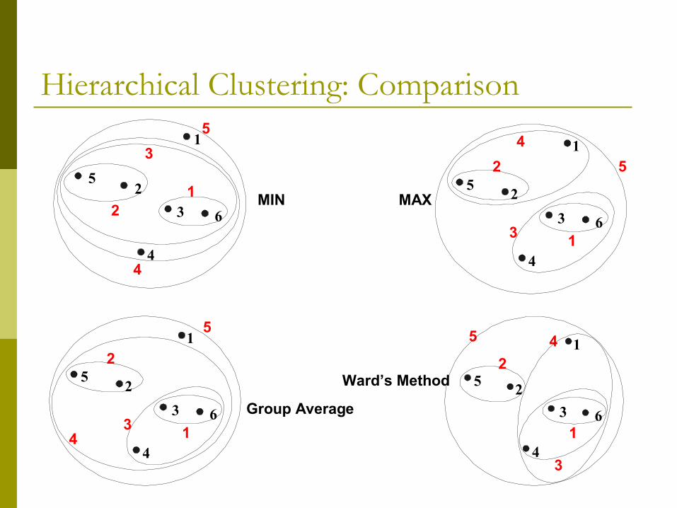
Hierarchical Clustering: Comparison

Group Average

Ward’s Method

1

23

4

5

61

2

5

3

4

MIN MAX

1

23

4

5

61

2

5

34

1

23

4

5

61

2 5

3

41

23

4

5

61

2

3

4

5

Hierarchical Clustering: Time and Space requirements O(N2) space since it uses the proximity

matrix. N is the number of points.

O(N3) time in many cases There are N steps and at each step the size,

N2, proximity matrix must be updated and searched

Complexity can be reduced to O(N2 log(N) ) time for some approaches

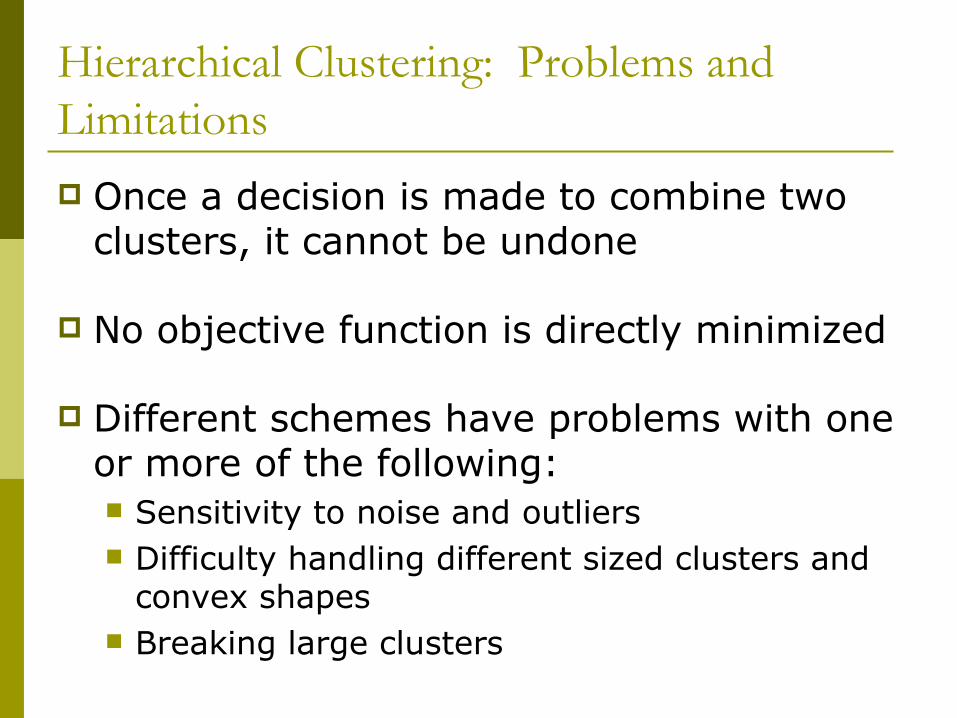
Hierarchical Clustering: Problems and Limitations Once a decision is made to combine two

clusters, it cannot be undone

No objective function is directly minimized

Different schemes have problems with one or more of the following: Sensitivity to noise and outliers Difficulty handling different sized clusters and

convex shapes Breaking large clusters

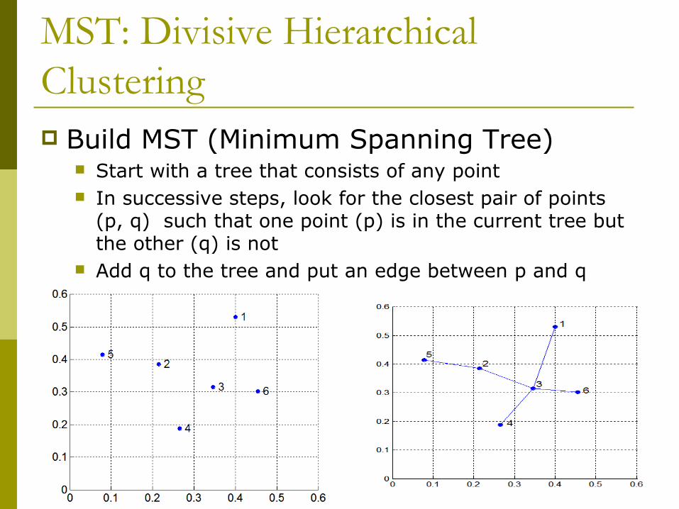
MST: Divisive Hierarchical Clustering Build MST (Minimum Spanning Tree)

Start with a tree that consists of any point In successive steps, look for the closest pair of points

(p, q) such that one point (p) is in the current tree but the other (q) is not

Add q to the tree and put an edge between p and q

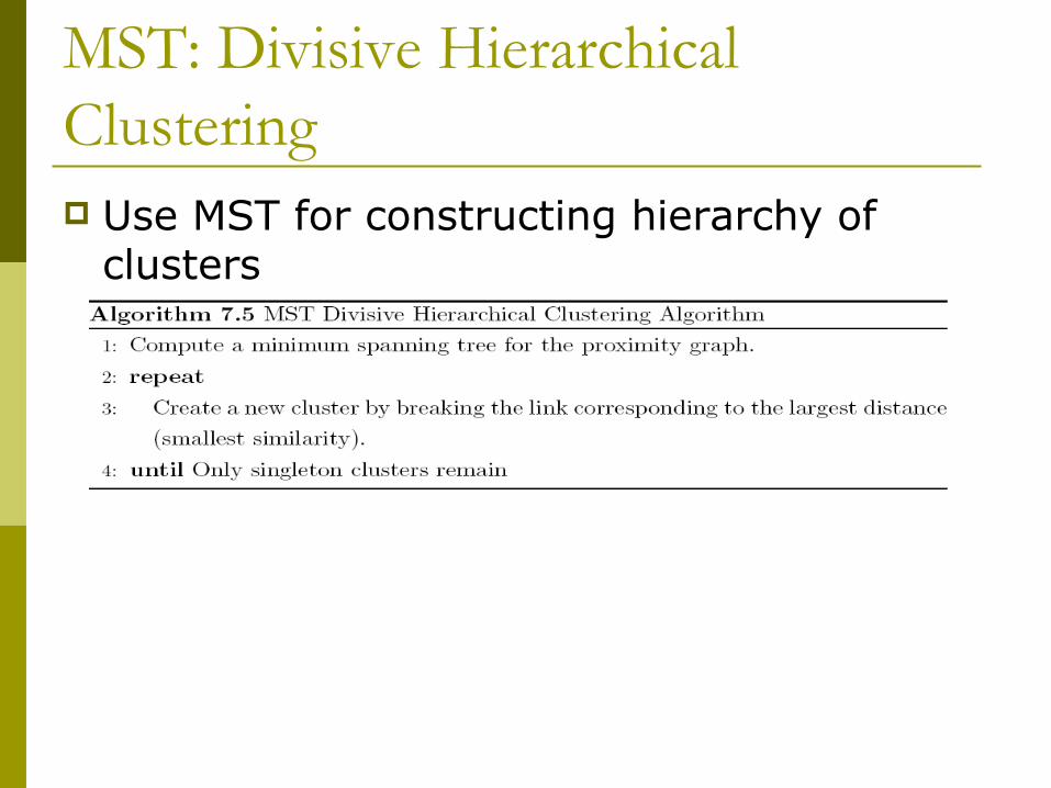
MST: Divisive Hierarchical Clustering Use MST for constructing hierarchy of

clusters

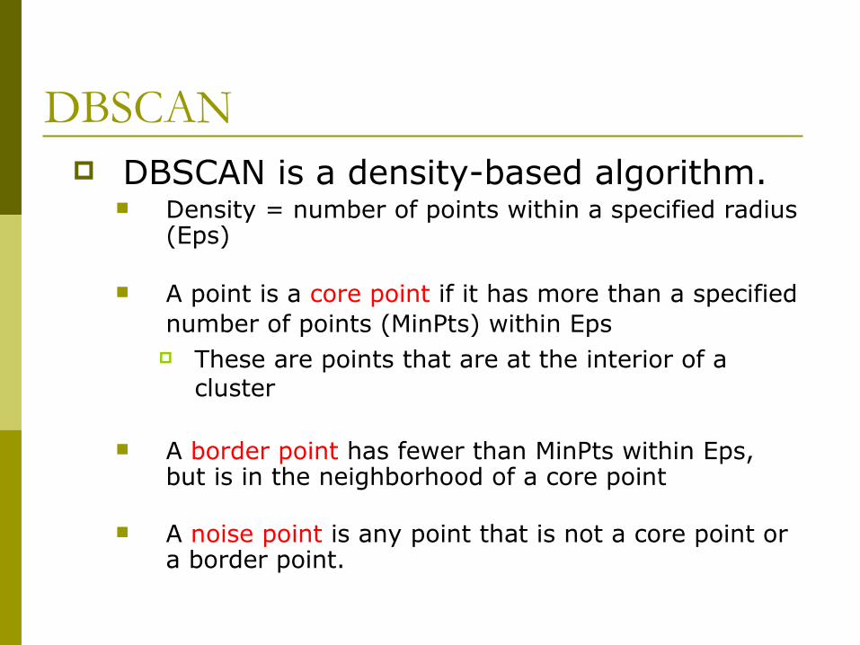
DBSCAN DBSCAN is a density-based algorithm.

Density = number of points within a specified radius (Eps)

A point is a core point if it has more than a specified number of points (MinPts) within Eps These are points that are at the interior of a

cluster

A border point has fewer than MinPts within Eps, but is in the neighborhood of a core point

A noise point is any point that is not a core point or a border point.

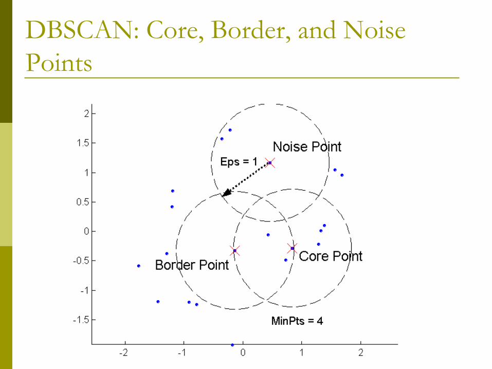
DBSCAN: Core, Border, and Noise Points

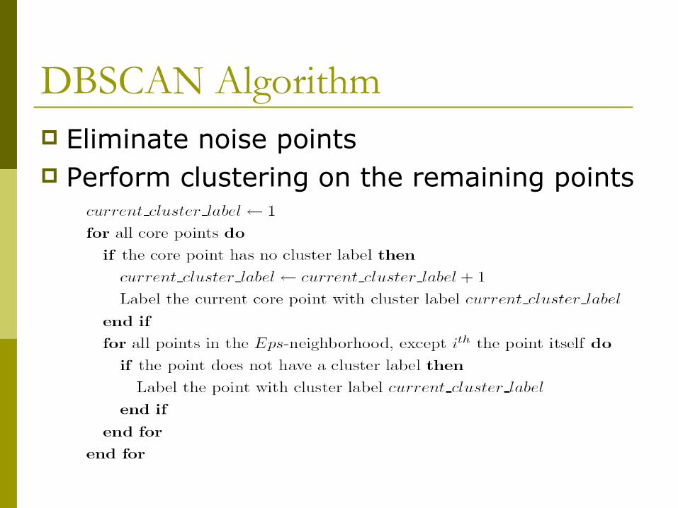
DBSCAN Algorithm Eliminate noise points Perform clustering on the remaining points

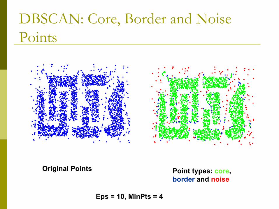
DBSCAN: Core, Border and Noise Points

Original Points Point types: core, border and noise

Eps = 10, MinPts = 4

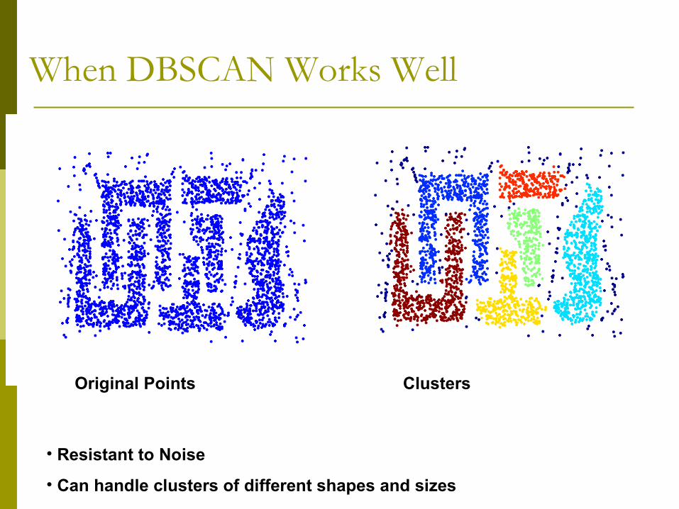
When DBSCAN Works Well

Original Points Clusters

• Resistant to Noise

• Can handle clusters of different shapes and sizes

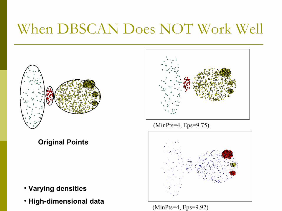
When DBSCAN Does NOT Work Well

Original Points

(MinPts=4, Eps=9.75).

(MinPts=4, Eps=9.92)

• Varying densities

• High-dimensional data

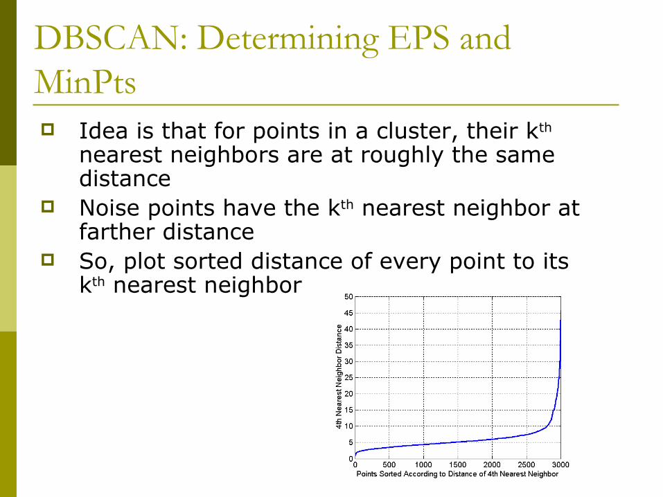
DBSCAN: Determining EPS and MinPts Idea is that for points in a cluster, their kth

nearest neighbors are at roughly the same distance

Noise points have the kth nearest neighbor at farther distance

So, plot sorted distance of every point to its kth nearest neighbor