closing the achievement gap in mathematics: evidence from ... · original research closing the...
TRANSCRIPT

ORI GINAL RESEARCH
Closing the achievement gap in mathematics: evidencefrom a remedial program in Mexico City
Emilio Gutierrez • Rodimiro Rodrigo
Received: 11 August 2013 / Revised: 31 July 2014 / Accepted: 7 October 2014 /
Published online: 11 November 2014
� The Author(s) 2014. This article is published with open access at Springerlink.com
Abstract This paper evaluates the impact of an intervention targeted at marginal-
izedlow-performance students in public secondary schools in Mexico City. The program
consisted in offering free additional math courses, taught by undergraduate students from
some of the most prestigious Mexican universities, to the lowest performance students in
a set of marginalized schools in Mexico City. We exploit the information available in all
students’ (treated and not treated by the program) transcripts enrolled in participating and
non-participating schools. Before the implementation of the program, participating
students lagged behind non-participating ones by more than a half base point in their GPA
(over 10). Using a difference-in-differences approach, we find that students participating
in the program observed a higher increase in their school grades after the implementation
of the program, and that the difference in grades between the two groups decreases over
time. By the end of the school year (when the free extra courses had been offered, on
average, for 10 weeks), participating students’ grades were not significantly lower than
non-participating students’ grades. These results provide some evidence that short and
low-cost interventions can have important effects on student achievement.
Keywords Impact evaluation � Remedial education programs � Difference-in-
differences estimators
JEL Classification C23 � I21 � I28 � O15
E. Gutierrez (&)
Centro de Investigacion Economica, Instituto Tecnologico Autonomo de Mexico, ITAM, Camino a
Sta. Teresa #930, Heroes de Padierna, 10700 Mexico DF. CP, Mexico
e-mail: [email protected]
R. Rodrigo
Department of Economic Productivity, Secretarıa de Hacienda y Credito Publico, Palacio Nacional,
06600 Mexico DF. CP, Mexico
e-mail: [email protected]
123
Lat Am Econ Rev (2014) 23:14
DOI 10.1007/s40503-014-0014-2

1 Introduction
While the evidence on the efficacy of different programs aimed at increasing a
population’s schooling accumulates, the evidence on the effectiveness of programs
targeted at improving school quality is not as vast. Existing evidence has measured
the impact of conditional transfer programs (Behrman et al. 2011), information
provision (Jensen 2010), school construction (Duflo 2001), and other school
resources, such as teachers (Banerjee et al. 2004) and text books (Glewwe et al.
2002) on school enrollment or schooling years.
However, studies finding that particular interventions increase school atten-
dance or schooling do not always find evidence that these programs improve
students’ performance on standardized tests. In other words, ‘‘students often seem
not to learn anything in the additional days that they spend at school’’ (Banerjee
et al. 2008). Such is the case of Mexico, where despite successful efforts to
increase schooling (e.g., Oportunidades), children’s cognitive skills have arguably
increased by very little or nothing (Behrman et al. 2011). In addition,
interventions aimed at improving school inputs, such as text books and number
of teachers, find very little or no effects on students’ performance (Banerjee et al.
2004; Glewwe et al. 2002).
Recently, more attention has been put into the design and evaluation of programs
aimed at improving learning. Examples of such interventions include Conditional
Cash Transfers programs like the one studied by (Barham et al. 2013) in Nicaragua,
and pedagogical strategies aimed at better matching teaching to students’ learning
needs, like the one studied in (Banerjee et al. 2008) and in this paper, specifically
targeted at the worst performing students within classrooms. However, their
effectiveness is likely to depend on their design and the setting in which they are put
in place.
This paper evaluates the impact on students’ grades of a low-cost intervention in
public secondary schools in Mexico City, which consisted in offering free additional
math courses to students lagging behind their peers in marginalized low-income
schools in Mexico City.
We exploit the information available in all students’ (treated and not treated by
the program) transcripts enrolled in participating and non-participating schools.
Before the implementation of the program, participating students lagged behind
non-participating ones by more than a half base point of their GPA (over 10). Using
a difference-in-differences approach, we find that students participating in the
program observed a higher increase in their school grades after the implementation
of the program, and that the difference in grades between the two groups decreased
over time. By the end of the school year (when the free extra courses had been
offered, on average, for 10 weeks), participating students’ grades were not
significantly lower than non-participating students’ grades.
After accounting for the presence of (i) mean reversion, and (ii) differences in
testing and grading among teachers, our results suggest that the impact on math
grades associated with the program is positive and significant in the order of 0.21
14 Page 2 of 30 Lat Am Econ Rev (2014) 23:14
123

and 0.26 standard deviations in the fourth and fifth partial exams.1 The estimated
impact is similar in magnitude to other studies’ findings. For example, Banerjee
et al. (2008) find that a similar intervention, the Balsakhi Program in India,
increased participating students’ grades by 0.14 standard deviations in the first
year.2
The paper is organized as follows. Section 2 reviews the recent literature that
analyzes similar interventions, describing their design and findings in detail.
Section 3 describes the setting in which the program evaluated in this paper was put
in place, and motivates the need for its evaluation. Section 4 describes the data and
the empirical strategy used in this paper. Results are presented in Sect. 5. Section 6
concludes.
2 Literature
Despite the growing number of programs targeting underperforming students in
different countries, there exists very little evidence on their effectiveness. Two
recent exceptions, which analyze similar interventions to the one studied here, are
Banerjee et al. (2008), and Lavy and Schlosser (2005).
Banerjee et al. (2008) evaluate a remedial education program that hired women
to teach third and fourth grade students in India lagging behind their peers in basic
literacy and math skills in small groups. The evaluation design for this intervention
used a sample of 15,000 students in two Indian cities, to which the treatment was
randomly assigned. The treatment consisted in offering additional courses taught by
an instructor (typically a young woman who received 2 weeks of training for this
purpose) to a subset of lower performing students from each of the treated
classrooms. These additional courses lasted for 2 h a day, took place during school
hours, and were taught to groups of 15–20 children. The courses covered basic
material that children were supposed to have learned in first and second grade.
Finally, as the one studied in this paper, the cost of this intervention was relatively
low, since teachers were local personnel trained for 2 weeks and paid 15 dollars per
month.
The authors look at the impact of the program on learning levels, measuring
learning using annual pre-intervention tests administered during the first few weeks
of the school year and post-intervention tests, administered at the end. They found
that it increased average test scores of all children in treatment schools by 0.14
standard deviations, mostly due to large gains experienced by children at the bottom
of the test-score distribution. Their results suggest that the remedial course program
1 In Mexico, grading throughout the school year is based on five evaluations (one every 2 months), called
‘‘examenes parciales’’. The final GPA is calculated as the simple average of these five exams’ grades.
Throughout the paper, we call each of these evaluations a ‘‘partial exam’’.2 The Balsakhi program provided schools with a teacher (local personnel paid 15 dollars a month) to
work for 2 h a day during the school year, with groups of 15–20 children in the third and fourth grades
identified as falling behind their peers. Banerjee et al. (2008) estimate improvements in average test
scores of 0.14 standard deviations in the first year, and 0.28 in the second.
Lat Am Econ Rev (2014) 23:14 Page 3 of 30 14
123
was more cost effective than hiring new teachers3 and than a computer-assisted
learning program implemented at the same time in a similar geographic area.4
Lavy and Schlosser (2005) evaluate the short-term effects of a remedial
education program, which provided additional instruction to underperforming high
school students in Israel. The program targeted tenth to twelfth graders in need of
additional help to pass the matriculation exams. As a control, they use a comparison
group of schools with similar characteristics to those treated (schools that enrolled
later in the program), and apply a difference-in-differences empirical strategy.
The intervention consisted in individualized instruction in small study groups of
up to five tenth, eleventh and twelfth graders. The main goal of these study groups
was, through individualized instruction based on underperforming students’ needs,
to increase their matriculation rate and enhance their scholastic and cognitive
abilities, self-image, and leadership aptitudes. The participants were chosen by their
teachers based on their perceived likelihood that each student could pass his or her
matriculation exam.
The evaluation focuses on the first year of implementation of the program. 4,100
students were affected by the intervention (one-fifth of all students in treated
schools).
The authors look for the effects of the program on matriculation status, which is a
comparable outcome for 12th graders. They find that the program raised the school
mean matriculation rate by 3.3% points, mainly through its impact on targeted
participants, rejecting the existence of externalities on their untreated peers.
In conclusion, as summarized in Kremer et al. (2013), programs that reduce the
costs of attending school and improve students’ health and the availability of
information may have large impacts on school attendance, although not necessarily
impacting their performance. Moreover, interventions that increase existing school
inputs, such as teachers and textbooks, have been shown to be generally ineffective.
However, programs that are tailored to each individual student’s learning needs,
such as remedial programs, not only have been shown to have large impacts on
students’ performance, but are also cost effective. Nevertheless, the effectiveness of
programs of this kind relies on a correct design and the context of their
implementation.
3 Mexico’s education system
Pre-college education in Mexico is divided into three main stages: primary or
elementary school, secondary school, and high school. Private schools must
cover the same curriculum as schools in the public system, and the content of
this curriculum is exclusively designed by the Ministry of Public Education
(Secretarıa de Educacion Publica, SEP) for the first nine grades (all of primary
3 A program reducing class size appears to have had little or no impact on test scores, and the remedial
course program costs 2.25 dollars per student per year.4 The computer-assisted learning program costs approximately 15.18 dollars per student per year,
including the cost of computers, assuming a 5-year depreciation.
14 Page 4 of 30 Lat Am Econ Rev (2014) 23:14
123

and secondary school). SEP shares the responsibility of designing the curriculum
and regulating private education at the high school level with the public
university system. Primary school lasts for 6 academic years, and is typically
attended by children aged 6–12. Secondary school and high school last three
academic years each. Unlike the United States, Mexico does not regulate the age
at which children can legally drop out of school. Instead, although the law is not
enforced, it is compulsory for all Mexicans to graduate from secondary school.
There exists a variety of different programs within both primary and secondary
public education in Mexico. Primary schools can be ‘‘general’’ (the most common),
indigenous (where courses are taught in indigenous languages), and community
schools (which target the most isolated communities and where students from
different grades generally share a classroom). In addition to general and community
schools, secondary schools can also be technical, ‘‘tele-secundarias’’ (which teach
the general program but through television and pre-recorded classes), and secondary
schools for adults (offered to individuals aged 15 or older who have completed their
primary education). After secondary school, there are 3 years of high school which
must be completed to attend college.
Table 1 shows some descriptive statistics about the Mexican education system,
obtained from the Mexican Institute for the Evaluation of Education (INEE). The
primary school system has nearly reached universal coverage. One hundred percent
of children aged 6–11 are enrolled in school. Secondary school, despite being
compulsory by law, does not show such high enrollment rates: 90 % of children
aged 12–14 are enrolled in school. Enrollment rates in high school are considerably
lower: only 60 % of children aged 15–17 are enrolled in school. Mexico City shows
slightly different enrollment rates: full enrollment in primary and secondary schools
and 86.7 % enrollment in high school.
It is then clear that the largest drop in enrollment rates, particularly in Mexico
City, takes place in the transition from secondary school to high school. However,
perhaps surprisingly, from all those students graduating from the last grade of
secondary school, nearly all of them enroll in high school, particularly in Mexico
City. The drop in enrollment seems then primarily a consequence of students’ low
performance in secondary school, which does not allow them to graduate and
continue with their education. 16 % of secondary school students do not pass the
grade in which they are enrolled. According to the standardized test applied by
INEE, ENLACE, in 2010, 40 % of secondary school students had insufficient
verbal skills and another 40 % just reached basic verbal skills’ levels; 53 % of
secondary school students had an insufficient math skills and another 34.7 % just
reached basic skills in math. According to the PISA 2009 test, 51 % of 15-year-
old students in Mexico’s educational system performed below level 2 in
mathematics (55 % in PISA 2012), and just 5 % ranked in the highest level
(5). It seems then crucial to design and evaluate interventions aimed at improving
students’ performance in secondary schools in Mexico, if increasing educational
attainment is a desired goal.
Lat Am Econ Rev (2014) 23:14 Page 5 of 30 14
123

4 The program
The program evaluated in this paper offers a remedial math course to low-
performance students enrolled in the last grade of secondary school from
marginalized schools in Mexico.
It was put in place by the representation of the SEP in Mexico City in
collaboration with the Laboratory of Initiatives for Development (LID), a local
NGO. It ran during the second half of the academic year 2009–2010, from April to
June 2010 in 33 schools in 11 different delegaciones.5
The remedial course was taught by a group of undergraduate students. There
were, in total, 55 advisors from three of the most prestigious universities in the
country: UNAM, ITAM, and UP. UNAM is a public university, while the other two
are private. These advisors fulfilled their ‘‘social service’’ requirement by
participating in this program. 480 h of social service activities (understood as
activities beneficial to society, the State or a university), after covering 70 % of the
undergraduate program credits, is a legal requirement for students to obtain a
college degree in Mexico. There is a wide range of activities that undergraduates
can do to fulfill this requirement, which go from being a research assistant,
participating in reforestation campaigns, or taking a job for a social organization or
government agency, with the latter being a common case. Employers are not legally
obliged to offer any remuneration for students during their social service. However,
generally, students do receive payments to cover their transportation needs (as was
the case for the students participating in the remedial program). The program seems
then easily replicable and, the extent to which it will be displacing social service
activities, its opportunity cost seems potentially low.
The program was advertised through the universities’ social service offices and
participating advisors enrolled voluntarily. Table 2 shows the distribution of
advisors recruited, by university and gender. Advisors’ attendance to the remedial
Table 1 Mexico’s education system. Descriptive Statistics (2010)
Percentage enrolled in school
All of Mexico Mexico City
Children aged 6–11 100 100
Children aged 12–14 90 100
Children aged 15–17 60.3 86.7
Continuation rate*
Primary to secondary 97 99
Secondary to high school 100? 100?
Source: INEE (2012)
* The continuation rate is calculated as the ratio between the number of individuals enrolling in one
education level in a given year divided by the total number of individuals graduating from the preceding
education level in the previous academic year. 100? indicates that this ratio was higher than one
5 Mexico City is divided into 16 delegaciones, which are the smallest administrative entities in the city.
14 Page 6 of 30 Lat Am Econ Rev (2014) 23:14
123

courses was controlled by the principals of all participating schools. In addition,
random visits to the remedial sessions were put in place by the implementing NGO
to verify their attendance to the remedial courses. In case the advisors were absent
for more than two consecutive sessions, they were not given the approximately 80
dollars for transportation costs that they were entitled to.
Prior to the intervention, the advisors were required to attend a brief but useful
training session of 4 h in total given by the Mexican Academy of Science, where
they had access to the mathematics syllabus at the secondary school level, a
previous final exam, and were instructed to look at children’s notebooks and
continuously ask the students for specific questions to regularly adapt the course’s
content to the group’s needs. The intervention in each of the participating schools
typically consisted of a meeting of two advisors with a group of up to 20
students, 2 days a week for 2 h, after school. This extra course focused on
helping children develop the mathematical skills needed to improve their grades
to pass the course.
The assignment of advisors to schools occurred as follows: (a) each of the
volunteers stated the neighborhood to which they would prefer to be assigned.
Table 2 Administrative data
Female Male Total
Advisors
Number of advisors 29 26 55
UNAM 10 7 17
ITAM 14 16 30
UP 5 3 8
Group size
Initial size 13.1 13.7 13.4
Final size 12.0 13.0 12.4
Sessions 11.2 7.7 9.9
Total hours 27.6 31.2 29.2
Schools
Type of secondary school
General 34
Technical 21
Shift
Morning school 18
Afternoon school 29
Both 8
Geographical location
North 14
South 7
East 30
Center 4
Lat Am Econ Rev (2014) 23:14 Page 7 of 30 14
123

(b) coordinators located three schools in the said neighborhood, choosing the worst
ranked in the ENLACE 2009 test who were willing to receive the program, (c) the
students ranked them according to their preferences and finally, taking into account
this information, coordinators assigned advisors to a single school.
Table 2 presents descriptive statistics for the outcome of the assignment of
advisors to schools. 34 advisors were assigned to general secondary schools and 21
to technical secondary schools; 18 taught the remedial courses to morning shift
students, and 29 to students in the afternoon shift. 8 advisors taught to students in
both shifts. Finally, from a total of 55 advisors, 14 volunteered at schools located in
northern Mexico City, 7 in the south, 30 in the east and 4 in the center.6
The assignment of students to the remedial course was decided by the schools’
principals. The general guidelines suggested by the coordinators of the program
were to identify students at risk of failing the school year, based on their
performance in the first two partial exams that they had already taken during that
academic year. The third partial exam had not yet been administered in any of the
schools at the time of the assignment of students to the remedial course.
The intervention began after the third partial exam on a date that varies from
school to school but in all cases before the fourth partial exam had been
administered, and lasted until the end of the school year.
Table 3 shows the fraction of students participating in the remedial course that
scored a grade average that was lower than the minimum passing grade after the first
two partial exams administered. 55 % of participating students had a passing grade
average in their first two partial exams, while 78 % of those not participating had a
passing grade average. The difference in this fraction is statistically significant from
zero.
The second panel in Table 2 shows that dropout rates from the remedial course
were low. At the beginning of the program, on average, 13.4 students attended the
course. The average remedial course class size by the end of the school year was
12.4 students.
5 Evaluation design
For the evaluation of this program, we collected detailed information on the math
grades obtained by a sample of participating and non-participating students in the
five partial exams administered during the academic year. As the program only
started after the third partial exam, we then have information on students’
performance before and after its implementation. There are two different groups of
non-participating students in our sample: non-participating students in schools in
which the program was put in place, and all students in a set of 60 schools (similar
in observable characteristics to the treated ones), in which the remedial course was
not offered.
6 The odd numbers reported in each school category are due to a few cases in which one single advisor
was assigned to a class, or to more than one school.
14 Page 8 of 30 Lat Am Econ Rev (2014) 23:14
123

Ta
ble
3S
um
mar
yst
atis
tics
on
mat
hap
pro
val
rate
so
f9
thg
rad
ers
Wit
hin
trea
ted
sch
ools
Bet
wee
nsc
ho
ols
All
the
sch
ools
inth
e
sam
ple
Tre
atm
ent
Con
tro
lS
imple
dif
fere
nce
s
(1–
2)
All
intr
eate
d
sch
ools
All
inn
on
-tre
ated
sch
ools
Sim
ple
dif
fere
nce
s
(1–
5)
(1)
(2)
(3)
(4)
(5)
(6)
(7)
Pre
-tre
atm
ent
0.5
59
[0.4
97]
0.7
84
[0.4
12
]
-0
.225
**
*[0
.01
7]
0.7
58
[0.4
28
]0
.76
3[0
.42
5]
-0
.209
**
*[0
.01
6]
0.7
62
[0.4
26]
Po
st-t
reat
men
t0
.806
[0.3
96]
0.8
30
[0.3
76
]
-0
.024
[0.0
15]
0.8
27
[0.3
78
]0
.84
0[0
.36
6]
-0
.032
*[0
.01
4]
0.8
37
[0.3
70]
Ob
serv
atio
ns
68
95
,258
–5
,94
71
6,2
78
–2
2,2
25
Th
ista
ble
giv
esth
ep
rob
abil
ity
of
app
rovin
gth
ey
ear
bef
ore
and
afte
rth
etr
eatm
ent
(co
nsi
der
ing
the
firs
ttw
og
rad
esan
dth
efi
ve
bim
estr
alg
rad
es,
resp
ecti
vel
y)
for
trea
tmen
tan
dco
mp
aris
on
stu
den
ts.
Co
lum
ns
(1)–
(3)
sho
wth
ep
rob
abil
ity
inth
etr
eatm
ent
gro
up
,th
eg
rou
po
fn
on
-tre
ated
stu
den
tsin
par
tici
pat
ing
sch
ools
,an
dth
e
dif
fere
nce
bet
wee
nth
em.C
olu
mn
s(4
)–(6
)sh
ow
the
pro
bab
ilit
yfo
ral
lst
ud
ents
intr
eate
dsc
ho
ols
,an
dal
lin
no
n-t
reat
edsc
ho
ols
,an
dth
esi
mp
led
iffe
ren
ceb
etw
een
the
last
gro
up
and
the
trea
tmen
tg
rou
p.
Co
lum
n(7
)sh
ow
sth
ep
rob
abil
ity
of
app
rove
the
yea
rfo
ral
lst
ud
ents
,tr
eate
dan
dn
on
-tre
ated
,fr
om
all
the
sch
oo
lsin
the
sam
ple
.S
tan
dar
d
erro
rsar
ein
bra
cket
s
*S
ign
ifica
nt
at1
0%
;*
*si
gn
ifica
nt
at5
%;
**
*si
gn
ifica
nt
at1
%
Lat Am Econ Rev (2014) 23:14 Page 9 of 30 14
123

In contrast with other studies listed above, the scores observed for each student
correspond to their grades on exams designed and graded by their specific teachers.
On one hand, this implies the possibility of high subjectivity on our performance
measure. However, as long as this subjectivity is teacher specific and not correlated
with the treatment within classrooms, we can evaluate to which extent treated
students caught up with their untreated peers.
Table 4 reports the average math grades in the five partial exams for students in
both the treatment and controls groups in our sample. Column 1 restricts the sample
to treated students. Column 2 restricts the sample to their classmates (non-treated
students in treated schools). As can be seen, the 689 treated students in the 32
participating schools had, on average, lower grades than their 5,258 non-treated
peers before the implementation of the program (first, second and third partial
grades). However, the difference between these groups decreases significantly for
the two partial exams after the program’s implementation. The difference in scores
for the fifth partial exam between treated and non-treated students is not statistically
different from zero (Column 3).
Column 4 shows the average score for all the 5,947 students in treatment schools,
and Column 5 shows the average scores for all the 16,278 students from the 60 non-
treated schools in our sample. Two facts are worth highlighting. First, non-treated
schools show higher average scores than treated schools, but the difference between
both does not seem to change considerably over time. As for the differences
between treated and non-treated students within treated schools, when comparing
treated students with all non-treated students in our sample, treated students reduce
the distance in average grades from non-treated ones after the implementation of the
program (Column 6).
These descriptive statistics suggest that treated students observe an important
increase in their exam grades after the implementation of the program, which allows
them to catch up with their peers by the last partial exam. However, they also show
important differences in levels for average grades between treated and non-treated
students. Determining if the closing of the grade gap is indeed a result of the
intervention requires a more refined analysis, which we describe in what follows.
6 Estimation strategy
The simplest version of our estimation strategy will consist in comparing the
average scores on all five partial exams, and the differences in them for the treated
and non-treated students. We present different results, changing the sample used
(excluding and including non-treated students in non-treated schools) and including
increasing controls. The basic regression estimated will be the following:
Scoreijt ¼X5
t¼1
;tPartialt þX5
t¼1
btTreatmenti � Partialt þ eijt ð1Þ
where Scoreijt measures the grade of student i, at school j, in partial exam t (one to
five); Partialt is a set of five dummy variables, taking a value of one for each period;
14 Page 10 of 30 Lat Am Econ Rev (2014) 23:14
123

Ta
ble
4S
um
mar
yst
atis
tics
on
aver
age
score
sof
9th
gra
der
sin
mat
h
Wit
hin
trea
ted
sch
ools
Bet
wee
nsc
ho
ols
All
the
sch
ools
inth
e
sam
ple
Tre
atm
ent
Co
ntr
ol
Sim
ple
dif
fere
nce
s
(1–
2)
All
intr
eate
d
sch
oo
ls
All
inn
on
-tre
ated
sch
ools
Sim
ple
dif
fere
nce
s
(1–
5)
(1)
(2)
(3)
(4)
(5)
(6)
(7)
Pre
-tre
atm
ent
Par
tial
16
.296
[1.2
73]
6.8
56
[1.4
24
]
-0
.560
**
*[0
.05
7]
6.7
97
[1.4
20
]6
.923
[1.5
33]
-0
.619
**
*[0
.05
8]
6.9
04
[1.5
05]
Par
tial
26
.261
[1.1
90]
6.9
18
[1.7
46
]
-0
.657
2*
**
[0.0
69]
6.8
66
[1.6
71
]6
.932
[1.7
56]
-0
.647
**
*[0
.06
8]
6.9
11
[1.7
33]
Par
tial
36
.222
[1.2
13]
6.6
35
[2.1
08
]
-0
.413
**
*[0
.08
2]
6.5
88
[2.0
29
]6
.807
[2.0
32]
-0
.556
**
*[0
.07
9]
6.7
61
[2.0
34]
Av
erag
ep
re-
trea
tmen
t
6.2
60
[1.0
47]
6.8
03
[1.4
80
]
-0
.544
**
[0.0
58]
6.7
58
[1.4
27
]6
.908
[1.5
50]
-0
.607
**
*[0
.05
9]
6.8
68
[1.5
06]
Po
st-t
reat
men
t
Par
tial
46
.511
[1.2
70]
6.6
45
[2.4
26
]
-0
.134
[0.0
94]
6.6
30
[2.3
22
]6
.751
[2.3
22]
-0
.204
**
[0.0
90
]6
.728
[2.3
22]
Par
tial
56
.718
[1.5
60]
6.6
95
[2.6
30
]
0.0
24
[0.1
03
]6
.698
[2.5
30
]6
.897
[2.5
16]
-0
.139
[0.0
98
]6
.863
[2.5
22]
Av
erag
ep
ost
-
trea
tmen
t
6.6
15
[1.2
09]
6.6
70
[2.4
36
]
-0
.056
[0.0
94]
6.6
94
[2.2
96
]6
.823
[2.3
04]
-0
.171
*[0
.08
9]
6.8
17
[2.3
11]
Ob
serv
atio
ns
68
95
,258
–5
,947
16
,27
8–
22
,22
5
Th
ista
ble
giv
esth
em
ean
sco
res
for
the
fiv
ep
arti
alte
sts
(an
dth
eav
erag
eo
fth
ete
stta
ken
bef
ore
and
afte
rth
ein
terv
enti
on
)fo
rtr
eatm
ent
and
com
par
ison
stud
ents
.
Co
lum
ns
(1)–
(3)
sho
wth
eav
erag
esc
ore
sin
the
trea
tmen
tg
rou
p,
the
gro
up
of
no
n-t
reat
edst
ud
ents
inp
arti
cip
atin
gsc
ho
ols
,an
dth
ed
iffe
ren
ceb
etw
een
the
two
gra
de
aver
ages
.C
olu
mn
s(4
)–(6
)sh
ow
the
aver
age
sco
res
for
all
stud
ents
intr
eate
dsc
ho
ols
,an
dal
ln
on
-tre
ated
stud
ents
inal
lsc
ho
ols
,an
dth
esi
mp
led
iffe
ren
ceb
etw
een
the
last
gro
up
and
the
trea
tmen
tg
rou
p.
Colu
mn
(7)
sho
ws
mea
nsc
ore
sfo
ral
lst
ud
ents
,tr
eate
dan
dn
on
-tre
ated
,fr
om
all
the
sch
ools
inth
esa
mple
.S
tan
dar
der
rors
are
inb
rack
ets
*S
ign
ifica
nt
at1
0%
;*
*si
gn
ifica
nt
at5
%;
**
*si
gn
ifica
nt
at1
%
Lat Am Econ Rev (2014) 23:14 Page 11 of 30 14
123

Treatmenti is a dummy variable that takes a value of one if student i is treated
(participates in the remedial courses); and eijt is an error term associated with
student i, at school j, in partial exam t.
The coefficients estimated for the dummies for each partial exam will measure
the average scores for the non-treated students in each of the five exams. The
coefficients estimated for the effect of the interactions between the partial exams
and the treatment variable measure the average differential in grades between
students in the treatment and the control groups in each period.
Treated and non-treated students are likely to be different in terms of their
scholastic achievement. The treatment was only introduced after the third period.
Given this, if our identification strategy is correctly measuring the causal impact of
the treatment on students’ scores, we would not expect to see any statistical
difference in the coefficients for the interaction between the treatment and the
period variables for the first three periods. As the constant term is excluded from the
regressions, the coefficient on these three variables will simply capture the
differences in grades between the treatment and control groups in the absence of the
remedial courses.
The measured impact of the remedial courses will then consist of comparing the
coefficient for the interaction between the treatment and period variables for the last
two periods, with those of the first three periods. This estimation strategy allows us
then to identify if the trends in exam grades were similar before the implementation
of the remedial program for the treatment and control groups, and also evaluate if its
effects increase or decrease between the fourth and fifth periods.
Given the program’s design, the conventional evaluation approach described by
Eq. (1) may yield misleading estimates of the effect of the intervention because of
two main concerns: (i) mean reversion, and (ii) differences in testing and grading
among teachers. The equation residuals can be thought as the sum of the following
components:
eijt ¼X5
t¼1
uijt � Partialt þ sj
where uijt is the transitory unobservable good or bad luck events experienced by
student i at school j during the partial exam t modifying her performance, and sj is
the school j permanent effect, like unobservable characteristics of teachers and
peers.
6.1 Mean reversion correction
As described above, the assignment of students to the remedial course was decided
by the school’s principal, who followed guidelines to identify students at risk of
failing the school year based on their performance on the first two partial exams.
The problem with evaluating interventions that select the treatment and control
groups based on previous test scores is that a single pre-program test scores
represent noisy measures of students’ performance, due to error variance.
14 Page 12 of 30 Lat Am Econ Rev (2014) 23:14
123

The reason is that there may be one-time events occurring during the exam such
as a simple flu, variation in the ingested amount of sugar, or other distractions that
may alter students’ performance. Hence, a student placing at the bottom or top of
the class distribution may do so due to a transitory testing noise, and may thus not be
indicative of her true performance.
If this is the case, as Chay et al. (2005) point out, if some students are assigned to
the treatment due to strong negative shocks to their performance in the first and
second partial exams, their pre-program grades will contain a strongly negative
error. Unless errors are perfectly correlated over time, one would expect scores in
subsequent partial exams to rise, even in the absence of the intervention. Thus, the
measured test score gains from a difference-in-differences analysis, as the
specification in Eq. (1) suggests, will reflect a combination of the true program
effect and spurious mean reversion.
To correctly identify the impact of the program, we need to eliminate sources of
spurious correlation between the change in partial exams’ grades and the grades
obtained before the intervention.
For this purpose, we first estimate a control function that includes a linear
function of the first partial exam to control for the negative shocks that students
could have experienced during the first exam. Specifically, we add to Eq. (1) the
interactions between the score in the first partial exam and the dummies of partial
exams 2–5. The estimated equation in this case will be:
Scoreijt ¼X5
t¼2
;tPartialt þX5
t¼2
btTreatmenti � Partialt
þX5
t¼2
ctScorei1 � Partialt þ eijt
ð2Þ
where Scoreit now stands for the grade of student i, at school j, in partial exam
t (from two to five), and Scorei1 measures student i’s score on the first partial exam.
The coefficients for the interaction between the grade in the first partial exam and
the dummy variables for each partial exam will control for mean reversion.
If our estimation strategy is correct, given that the program only started after the
third midterm exam, if the student in the treatment group experienced a temporary
negative shock during this first partial exam, we would expect the coefficients for
the interaction of the treatment dummy with period 2 and 3 dummies to reflect the
real gap among groups (being statistically of the same magnitude for both periods) if
there is any. And so, if the coefficients for the interaction of the treatment with
period 4 and 5 dummies get reduced in comparison to that associated with the pre-
program situation, then this reduction could be attributed to the program. This
specification concretely allows us to relax the implicit assumption of Eq. (1),
E uijt
� �¼ 0; 8i; 8j; 8t, and allows for potential transitory shocks suffered in period 1
leading to mean reversion.
To better control for the possibility of mean reversion, we also estimate a control
function with a cubic polynomial in the first partial exam:
Lat Am Econ Rev (2014) 23:14 Page 13 of 30 14
123

Scoreit ¼X5
t¼2
;tPartialt þX5
t¼2
btTreatmenti � Partialt
þX5
t¼2
ctScorei1 � Partialt þX5
t¼2
utScore2i1 � Partialt
þX5
t¼2
qtScore3i1 � Partialt þ eit
ð2:aÞ
where Scorei12 and Scorei1
3 are the square and cubic of the grade of student i in partial exam
1. The coefficients for the interaction between the linear, square and cubic of the grade in
the first partial exam and the dummy variables for each partial exam will control for mean
reversion, allowing us to relax the assumption that it is linear. The expectations over the
resulting estimations would be exactly as described for the linear case.
6.2 Ability of the students to improve
Nonetheless, concerns related to mean reversion can still remain. The school’s
principals assigned students to the treatment with more information than just their
performance on the first partial exam. It is possible that their selection rule included in
fact the observed trend in grades for the first two evaluations, for example. Therefore,
they would tend to select students who worsen in the second exam compared to the first
one and leave without treatment those who probably would apparently be able to
improve on their own, given their noisy second partial grade. If this was the case, the
estimated coefficients for the interaction between the dummies for the second and third
partial exams and the treatment dummy are likely to differ from zero.
Our estimation strategy can be further refined to control for this difference in the
apparent ability of the students to improve. In particular, we can control for the
change in scores between the first and second partial exams for each student,
interacted with the period dummies (three to five). Specifically, the regression
estimated would be:
Scoreit ¼X5
t¼3
;tPartialt þX5
t¼3
btTreatmenti � Partialt
þX5
t¼3
ctScorei1 � Partialt
þX5
t¼3
ptðScorei2 � Scorei1Þ � Partialt þ eit
ð3Þ
Further, it is possible that more than just the initial grade and the change in
grades between the first and second partial exams were used by the principals to
assign students to the treatment. We can then also include the triple interaction
between the initial grade, the change in grades between periods one and two, and the
dummy variables for each period, three to five:
14 Page 14 of 30 Lat Am Econ Rev (2014) 23:14
123

Scoreijt ¼X5
t¼3
;tPartialt þX5
t¼3
btTreatmenti � Partialt
þX5
t¼3
ctScorei1 � Partialt þX5
t¼3
ptðScorei2 � Scorei1Þ � Partialt
þX5
t¼3
otðScorei2 � Scorei1Þ � Scorei1 � Partialt þ eijt
ð4Þ
Equations (3) and (4) allow us to further relax the identification assumption nec-
essary for the estimates from Eq. (2) to measure the effect of the program.
Now, the assumption would be that treated and non-treated students with similar
grades in the first partial exam and similar changes in grades between the first and
second exams were equally likely selected to receive the intervention. Moreover,
there is no further assumption needed with respect to the existence of noise when
measuring the pre-program performance of the students, because this specification
controls for that, allowing the occurrence of transitory shocks.
The idea now is that apart from the possibility of having experienced a negative
transitory shock during the first partial, it could also be the case that students in the
treatment (or in the control) group experienced a negative (or positive) shock during
the second exam correlated with the shock in the previous one. In this case, we
would observe improvements in grades on further exams even in the absence of the
program, caused by mean reversion. Therefore, we need to add to Eq. 2 the
interactions between the score in the second partial exam and the dummies of partial
exams 3–5.7 This specification allows us to further relax the assumption in Eq. (1),
E uijt
� �¼ 0; 8i; 8j; 8t, and allows for potential transitory shocks suffered in periods 1
and 2 leading to mean reversion .
Also, note that adding Scorei2 or ðScorei2 � Scorei1Þ to Eq. (2) solves the
concern about mean reversion explained in the previous paragraph, since the
difference ðScorei2 � Scorei1Þ is a linear transformation of Scorei2. Therefore, the
specification suggested by Eq. (3) not just controls for the ability of students to
improve, but also for mean reversion in a more satisfactory way.
If this specification is correct, we would expect the coefficients for the interaction
of the treatment and the third period dummy to be not significantly different from
zero, as the program had not been implemented by that time. And the coefficients
for the interaction of the treatment with periods 4 and 5 dummies would reflect the
impact associated with the program.
7 Specifically, we would need to estimate the following equation:
Scoreit ¼P5
t¼2
;tPartialt þP5
t¼2
btTreatmenti � Partialt
þP5
t¼2
ctScorei1 � Partialt þP5
t¼2
utScorei2 � Partialt þ eit
Lat Am Econ Rev (2014) 23:14 Page 15 of 30 14
123

6.3 Differences in testing and grading among teachers
An important difference between this paper and similar studies (listed above) is that
the scores observed for each student correspond to their grades on exams designed
and graded by their specific teachers and not to standardized tests. In this section, we
analyze the advantages and disadvantages of considering this measure of students’
performance.
Standardized tests are uniform in subject matter, format, administration, and
grading procedure across all test takers, while a course grade might depend on a
particular teacher’s judgment. However, course grades and standardized tests both
reflect students’ skills and knowledge, and are thus generally highly correlated
(Willingham et al. 2002).
Trying to provide an explanation to why these two evaluation tools are not
entirely interchangeable, recent literature has underlined aspects of personality that
seem essential to earning strong course grades because of what is required of
students to earn them. Almlund et al. (2011) analyze how the contribution of
personality to performance varies among these two evaluation methods.
One key point is that despite the power of standardized achievement tests to
predict later academic and occupational outcomes (for example in Kuncel and
Hezlett (2007); Sackett, et al. (2008)), cumulative high school GPA predicts
graduation from college much better than standardized test scores do (as shown by
Bowen et al. (2009)). Similarly, high school GPA more powerfully predicts college
rank-in-class (Bowen et al. 2009; Geiser and Santelices 2007).
Duckworth et al. (2012) compare the variance explained in standardized test
scores and GPA at the end of the school year by self-control and intelligence
measured at the beginning of the school year. In a sample of children, they found
that fourth graders’ self-control was a stronger predictor of ninth graders’ GPA than
fourth graders’ IQ. At the same time, fourth graders’ self-control was a weaker
predictor of ninth graders’ standardized test scores than was fourth graders’ GPA.
Similarly, Oliver et al. (2007) found that parent and self-reported ratings of
distractibility at age 16 predicted high school and college GPA, but not SAT test
scores.
Given these arguments, analyzing grades instead of standardized scores seems to
be a better idea to measure the impact of the program according to the initial
objective. Unfortunately, the possibility of high subjectivity on our performance
measure still remains. However, as long as this subjectivity is teacher specific and
not correlated with the treatment within classrooms, we can evaluate to what extent
treated students caught up with their untreated peers.
Taking advantage of the panel structure of our data, which contains a measure of
each student performance in five different periods, we can control by school level
fixed effects. In this way, we relax the implicit assumption in every previous
specification that EðsjÞ ¼ 0; 8j, in words, we are capturing the differences in
students’ scores driven by differences across school characteristics, such as the
teacher’s specific preferences for testing and grading.
14 Page 16 of 30 Lat Am Econ Rev (2014) 23:14
123

7 Results
Results for all specifications described above are presented in Tables 5 and 6.
Table 5 uses all non-treated students in participating schools as the control group,
while Table 6 includes all non-treated students as a control (including those in the
60 non-participating schools for which we have information). Columns 1, 2, 3 and 4
show the results for the specification described in the equation with the same
number in the previous section.
The results of estimating Eq. (1) are shown in Column 1 of Tables 5 and 6. As
can be seen, the coefficients for the interaction between the treatment and partial
variables are negative and significantly different from zero for the first three partials
both when restricting the sample to all students in treated schools (Table 5) and
when including all students in treated and non-treated schools (Table 6). The
coefficient for the interaction between the treatment dummy and partial 4 is
significantly lower in magnitude than those for the first three partial exams. The
grade gap between the treated and non-treated students seems then to decrease after
the implementation of the program. Perhaps more interestingly, the coefficient for
the interaction between the treatment and period 5 dummies is close to zero and
insignificant when the sample is restricted to students in treated schools (suggesting
that the program might have completely closed the performance gap between the
two groups after 3 months of its implementation). When including students in non-
treated schools in the sample, this coefficient remains significantly negative,
although still smaller in magnitude than that for partial 4.
Consistently, when testing whether the coefficients of the interactions between
the treatment dummy and the partial exam dummy variables are statistically
different for both control groups (non-treated students within treated schools and in
all schools), reported in Table 7, we fail to reject that the estimated coefficients for
the interaction with partial 1 and the interaction with partial 2 are equal, and the
same with the estimated coefficients for the interaction with partial 2 and the
interaction with partial 3. Nevertheless, based on a confidence level of 95 %, the F
test rejects that the estimated coefficients for the interaction between the treatment
dummy with partial 3 and the interaction with partial 4 are equal (when doing this
exercise for all schools, we get the same result but with a confidence level of 90 %),
and the same result is obtained when testing for the interaction with partial 3 and the
interaction with partial 5. We fail to reject that the estimated coefficients for the
interaction with partial 4 and the interaction with partial 5 are equal.
Nevertheless, as stated above, for this empirical strategy to correctly identify the
program’s effects, we would expect the trends in grades between treated and non-
treated students before the implementation of the program to not be different.
Figure 1, which shows the regression results graphically, suggests that this is
perhaps not the case. Grades for treated students seem to increase (relative to non-
treated students’ grades) since before the program’s implementation (period 3).
The following three columns in both tables present the regression results for the
specifications described in Eqs. (2)–(4), respectively. Column 2 compares scores in
partial exams 2–5 of students from the treatment and control groups controlling for
the score in the first partial exam. As can be seen, students in the treatment group, by
Lat Am Econ Rev (2014) 23:14 Page 17 of 30 14
123

Ta
ble
5T
reat
men
tef
fect
so
nth
eav
erag
em
ath
score
sw
ithin
trea
ted
schools
(1)
(2)
(3)
(4)
Par
tial
16
.863
**
*[0
.02
8]
Par
tial
26
.945
**
*[0
.02
8]
2.1
08
**
*[0
.12
6]
Par
tial
36
.663
**
*[0
.02
7]
2.3
90
**
*[0
.12
6]
0.9
91
**
*[0
.12
8]
0.9
92
**
*[0
.12
8]
Par
tial
46
.679
**
*[0
.02
7]
2.2
53
**
*[0
.12
6]
0.8
02
**
*[0
.12
8]
0.8
10
**
*[0
.12
8]
Par
tial
56
.729
**
*[0
.02
8]
2.5
05
**
*[0
.12
6]
0.9
45
**
*[0
.12
8]
0.9
52
**
*[0
.12
8]
Tre
atm
ent
*P
arti
al1
-0
.56
9*
**
[0.0
82]
Tre
atm
ent
*P
arti
al2
-0
.67
8*
**
[0.0
82]
-0
.278
**
*[0
.07
9]
Tre
atm
ent
*P
arti
al3
-0
.43
8*
**
[0.0
81]
-0
.084
[0.0
79
]0
.10
0[0
.07
7]
0.1
00
[0.0
77]
Tre
atm
ent
*P
arti
al4
-0
.16
2*
*[0
.08
1]
0.2
05
**
*[0
.07
9]
0.3
96
**
*[0
.07
7]
0.3
93
**
*[0
.07
7]
Tre
atm
ent
*P
arti
al5
-0
.01
3[0
.08
1]
0.3
37
**
*[0
.07
9]
0.5
43
**
*[0
.07
7]
0.5
40
**
*[0
.07
7]
Con
tro
lsb
yP
arti
al1
gra
de
No
Yes
Yes
Yes
Con
tro
lsb
ytr
end
sin
gra
des
bef
ore
the
trea
tmen
tN
oN
oY
esY
es
Con
tro
lsb
yth
ein
tera
ctio
no
ftr
end
san
dg
rad
ein
Par
tial
1N
oN
oN
oY
es
Ob
serv
atio
ns
29
,41
02
3,5
28
17
,64
61
7,6
46
R-s
qu
ared
0.9
20
.93
0.9
30
.93
This
table
report
sth
ees
tim
ates
of
the
trea
tmen
tef
fect
assp
ecifi
edin
Eq.(1
,2,3,an
d4),
pre
sen
ted
inth
esa
me
ord
erin
Co
lum
ns
(1)–
(4),
tak
ing
all
the
no
n-t
reat
edst
ud
ents
of
the
trea
ted
sch
ools
asth
eco
mp
aris
on
gro
up
.S
tan
dar
der
rors
are
inb
rack
ets
*S
ign
ifica
nt
at1
0%
;*
*si
gn
ifica
nt
at5
%;
**
*si
gn
ifica
nt
at1
%
14 Page 18 of 30 Lat Am Econ Rev (2014) 23:14
123

Ta
ble
6T
reat
men
tef
fect
so
nth
eav
erag
em
ath
score
sfo
ral
lth
esa
mple
’ssc
hools
(1)
(2)
(3)
(4)
Par
tial
16
.923
**
*[0
.01
4]
Par
tial
26
.931
**
*[0
.03
9]
2.0
26
**
*[0
.05
9]
Par
tial
36
.807
**
*[0
.02
3]
1.9
89
**
*[0
.06
2]
0.6
08
**
*[0
.05
9]
0.6
12
**
*[0
.06
0]
Par
tial
46
.751
**
*[0
.01
3]
1.8
09
**
*[0
.05
9]
0.4
57
**
*[0
.05
9]
0.4
63
**
*[0
.06
0]
Par
tial
56
.897
**
*[0
.01
4]
2.3
17
**
*[0
.05
5]
0.9
51
**
*[0
.05
6]
0.9
63
**
*[0
.05
7]
Tre
atm
ent
*P
arti
al1
-0
.62
8*
**
[0.0
79]
Tre
atm
ent
*P
arti
al2
-0
.66
4*
**
[0.0
78]
-0
.219
**
*[0
.07
3]
Tre
atm
ent
*P
arti
al3
-0
.58
2*
**
[0.0
78]
-0
.145
**
[0.0
72
]0
.00
5[0
.07
0]
0.0
04
[0.0
70]
Tre
atm
ent
*P
arti
al4
-0
.23
4*
**
[0.0
78]
0.2
15
**
*[0
.07
3]
0.3
61
**
*[0
.07
0]
0.3
59
**
*[0
.07
0]
Tre
atm
ent
*P
arti
al5
-0
.18
0*
*[0
.07
8]
0.2
36
**
*[0
.07
3]
0.3
84
**
*[0
.07
0]
0.3
82
**
*[0
.07
0]
Con
tro
lsb
yP
arti
al1
gra
de
No
Yes
Yes
Yes
Con
tro
lsb
ytr
end
sin
gra
des
bef
ore
the
No
No
Yes
Yes
Con
tro
lsb
yth
ein
tera
ctio
no
ftr
end
san
dg
rad
ein
Par
tial
1N
oN
oN
oY
es
Ob
serv
atio
ns
11
0,0
05
88
,00
46
6,0
03
66
,00
3
R-s
qu
ared
0.9
20
.93
0.9
40
.94
This
table
report
sth
ees
tim
ates
of
the
trea
tmen
tef
fect
assp
ecifi
edin
Eq.(1
,2,3,an
d4),
pre
sen
ted
inth
esa
me
ord
erin
Co
lum
ns
(1)–
(4),
tak
ing
all
the
no
n-t
reat
edst
ud
ents
of
the
sch
ools
inth
esa
mple
asth
eco
mp
aris
on
gro
up
.S
tan
dar
der
rors
are
inb
rack
ets
*S
ign
ifica
nt
at1
0%
;*
*si
gn
ifica
nt
at5
%;
**
*si
gn
ifica
nt
at1
%
Lat Am Econ Rev (2014) 23:14 Page 19 of 30 14
123

the fifth partial exam, had experienced a 0.33 point increase in their grades relative
to their non-treated peers (Table 5) and a 0.24 points increase relative to the whole
sample of non-treated students. This change is roughly equivalent to half the grade
gap between the groups in their first partial exam. However, it is worth noting that
the coefficient on the interaction between the treatment dummy and the second
period is, for both samples, negative and statistically different from zero, but a
closing in the gap is still observed by the third period, when the program had not yet
begun. Adding the interaction between the first score and the period dummies does
5.8
6
6.2
6.4
6.6
6.8
7
1 2 3 4 5
Treatment Control 1
-0.7000-0.6000-0.5000-0.4000-0.3000-0.2000-0.10000.00000.1000
1 2 3 4 5
Diffs
5.8
6
6.2
6.4
6.6
6.8
7
1 2 3 4 5Treatment Control2
-0.7-0.6-0.5-0.4-0.3-0.2-0.1
01 2 3 4 5
Diffs
Fig. 1 Trends in partial grades between treatment groups. The left panel shows the average test scoresfor treated and untreated students in treatment schools. The right panel includes non-treated schools in thecontrol group
Table 7 F tests of differences on treatment effects across partial exams
Null hypothesis Treated schools All sample’s schools
F test P value F test P value
Partial 1 = Partial 2 0.900 0.342 0.100 0.747
Partial 2 = Partial 3 4.330 0.037 0.550 0.460
Partial 3 = Partial 4 5.690 0.002 9.760 0.002
Partial 3 = Partial 5 13.550 0.000 13.050 0.000
Partial 4 = Partial 5 1.680 0.195 0.240 0.626
Observations 29,400 110,005
This table presents the F test and P values’ result of testing the null hypothesis of estimated coefficients
for the treatment effects of each couple of partial exams to be equal. First two columns for the regressions
run for treated schools (reported in Table 5), the last two for those run for all sample’s school (in Table 6)
14 Page 20 of 30 Lat Am Econ Rev (2014) 23:14
123

not seem to fully solve the problem of mean reversion caused by the use of a noisy
measure of the students’ pre-treatment performance.
The last two columns in Tables 5 and 6 include further controls measuring
students’ performance in the first two partial exams. The results are quantitatively
similar when excluding or including (Columns 3 and 4) the interaction between the
grade in the first partial and the change in grades between the first and the second
exam as controls. Once we include all the observable information that the principals
had at the moment of selecting the treated students (the scores in partial 1 and partial
2, and the difference between them), the coefficient of the interaction between the
treatment dummy and the score in the third partial exam is insignificantly different
from zero. Students’ grades are then uncorrelated with the treatment before the
implementation of the program. With this specification, the difference in grades
between treated students and their non-treated peers (Table 5) decreases by 0.54
points by the fifth partial exam. This magnitude is very close to the grade gap in the
first partial exam, suggesting that the grade gap between treated students and their
peers was fully closed by the fifth partial exam. The same estimate using all non-
treated students in our sample as the control group (Table 6) suggests that the grade
gap was closed by 0.38 points by the fifth partial exam.
Tables 8 and 9 are analogous to Tables 5 and 6 but include school fixed effects to
correct by differences in testing and grading among teachers.8 The estimated
coefficients increase with respect to those without fixed effects (when it was 0.54),
to 0.66 points by the fifth partial when using the non-treated students in treated
schools as the control group.
Tables 10 and 11 present the results of the same specifications, splitting the
sample into boys and girls, respectively, and using the non-treated students in
treatment schools as the control group. According to the results of specification (1),
in both tables, the differences between treated and untreated boys’ and girls’ scores
in the first three partial exams are similar in magnitude, and the decreasing pattern
in this gap in the fourth and fifth partial exams documented for the full sample
remains for both groups. Looking at the graphed magnitudes in Fig. 2, it seems that
the changes in grades are larger for boys than girls, although it could be an artifact
of larger mean reversion in the boys’ sample, as suggested by the reduction in the
gap in the third partial exam, before the remedial course had been offered.
When including further controls and school fixed effects, the difference in grades
between treated students and their non-treated peers decreases by 0.73 points by the
fifth partial exam for boys, and by 0.56 points for girls.
Finally, to be able to compare the results of this low-cost program with the
impact of other interventions, Table 12 reports our results in standard deviations
taking the untreated students in treatment schools as the control group. The
estimations correspond exactly to those from Table 8 but with standardized
variables. Here, the estimated impact amounts to 0.26 standard deviations.
8 This exercise was made at the school level and not at class level as was suggested in the Evaluation
Design section, due to data limitations (we count with school identifier but not class identifier).
Nevertheless, according with the educational authorities, it is always the same teacher who teaches the
same subject to all classes in a school (but rare exceptions). In which case, school or class fixed effects
estimations would equally correct for differences in testing and grading among teachers.
Lat Am Econ Rev (2014) 23:14 Page 21 of 30 14
123

Ta
ble
8T
reat
men
tef
fect
so
nth
eav
erag
em
ath
score
sw
ithin
trea
ted
schools
,F
Esc
hools
(1)
(2)
(3)
(4)
Par
tial
16
.859
**
*[0
.20
8]
Par
tial
26
.941
**
*[0
.16
5]
1.7
26
**
*[0
.27
3]
Par
tial
36
.658
**
*[0
.07
6]
2.0
07
**
*[0
.34
8]
0.6
38
**
*[0
.20
4]
0.6
37
**
[0.2
15]
Par
tial
46
.674
**
*[0
.06
7]
1.8
70
**
*[0
.35
60
.448
**
*[0
.20
3]
0.4
56
**
[0.1
34]
Par
tial
56
.724
**
*[0
.10
1]
2.1
23
**
*[0
.36
0]
0.5
91
**
[0.2
92]
0.5
97
**
[0.2
02]
Tre
atm
ent
*P
arti
al1
-0
.527
**
[0.2
05]
Tre
atm
ent
*P
arti
al2
-0
.637
**
*[0
.17
8]
-0
.095
[0.1
08
]
Tre
atm
ent
*P
arti
al3
-0
.396
*[0
.20
3]
0.0
99
[0.1
46]
0.2
16
[0.1
15]
0.2
15
[0.1
16]
Tre
atm
ent
*P
arti
al4
-0
.121
[0.2
05]
0.3
87
**
*[0
.15
8]
0.5
11
**
*[0
.12
3]
0.5
07
**
*[0
.12
3]
Tre
atm
ent
*P
arti
al5
0.0
29
,0
.20
80
.520
**
*[0
.17
3]
0.6
58
**
*[0
.14
2]
0.6
55
**
*[0
.14
3]
Con
tro
lsb
yP
arti
al1
gra
de
No
Yes
Yes
Yes
Con
tro
lsb
ytr
end
sin
gra
des
bef
ore
the
trea
tmen
tN
oN
oY
esY
es
Con
tro
lsb
yth
ein
tera
ctio
no
ftr
end
s&
gra
de
inP
arti
al1
No
No
No
Yes
Ob
serv
atio
ns
29
,41
02
3,5
28
17
,64
61
7,6
46
R-s
qu
ared
0.9
20
.93
0.9
40
.94
Th
ista
ble
rep
ort
sth
ees
tim
ates
of
the
trea
tmen
tef
fect
assp
ecifi
edin
Eq
.(1
,2,3
,an
d4),
pre
sen
ted
inth
esa
me
ord
erin
Colu
mn
s(1
)–(4
),ta
kin
gal
lth
en
on
-tre
ated
stu
den
ts
of
the
sch
ools
inth
esa
mple
asth
eco
mp
aris
on
gro
up
.S
tan
dar
der
rors
are
inb
rack
ets
*S
ign
ifica
nt
at1
0%
;*
*si
gn
ifica
nt
at5
%;
**
*si
gn
ifica
nt
at1
%
14 Page 22 of 30 Lat Am Econ Rev (2014) 23:14
123

Ta
ble
9T
reat
men
tef
fect
so
nth
eav
erag
em
ath
score
sfo
ral
lth
esa
mple
’ssc
hools
,F
Esc
hools
(1)
(2)
(3)
(4)
Par
tial
16
.91
9*
**
[0.0
36]
Par
tial
26
.92
7*
**
[0.0
33]
1.9
29
**
*[0
.11
7]
Par
tial
36
.80
3*
**
[0.0
46]
1.8
91
**
*[0
.12
2]
0.1
51
**
*[0
.07
1]
0.5
87
**
[0.0
71]
Par
tial
46
.74
7*
**
[0.0
58]
1.7
11
**
*[0
.14
1]
0.4
35
**
*[0
.09
4]
0.4
38
**
*[0
.09
3]
Par
tial
56
.89
3*
**
[0.0
65]
2.2
20
**
*[0
.17
0]
0.4
94
**
*[0
.10
3]
0.9
37
**
*[0
.10
3]
Tre
atm
ent
*P
arti
al1
-0
.501
**
[0.2
12]
Tre
atm
ent
*P
arti
al2
-0
.537
**
*[0
.17
8]
-0
.008
[0.1
37]
Tre
atm
ent
*P
arti
al3
-0
.455
**
[0.1
87]
0.0
67
[0.1
34
]0
.221
*[0
.12
3]
0.2
18
*[0
.12
3]
Tre
atm
ent
*P
arti
al4
-0
.107
[0.1
89]
0.4
26
**
*[0
.13
6]
0.5
77
**
*[0
.12
1]
0.5
74
**
*[0
.12
1]
Tre
atm
ent
*P
arti
al5
-0
.053
[0.1
83]
0.4
47
**
*[0
.15
5]
0.5
99
**
*[0
.14
3]
0.5
96
**
*[0
.14
3]
Con
tro
lsb
yP
arti
al1
gra
de
No
Yes
Yes
Yes
Con
tro
lsb
ytr
end
sin
gra
des
bef
ore
the
trea
tmen
tN
oN
oY
esY
es
Con
tro
lsb
yth
ein
tera
ctio
no
ftr
end
san
dg
rad
ein
Par
tial
1N
oN
oN
oY
es
Ob
serv
atio
ns
11
0,0
05
88
,00
46
6,0
03
66
,00
3
R-s
qu
ared
0.9
20
.93
0.9
40
.94
Th
ista
ble
rep
ort
sth
ees
tim
ates
of
the
trea
tmen
tef
fect
assp
ecifi
edin
Eq
.(1
,2,3
,an
d4),
pre
sen
ted
inth
esa
me
ord
erin
Colu
mn
s(1
)–(4
),ta
kin
gal
lth
en
on
-tre
ated
stu
den
ts
of
the
sch
ools
inth
esa
mple
asth
eco
mp
aris
on
gro
up
.S
tan
dar
der
rors
are
inb
rack
ets
*S
ign
ifica
nt
at1
0%
;*
*si
gn
ifica
nt
at5
%;
**
*si
gn
ifica
nt
at1
%
Lat Am Econ Rev (2014) 23:14 Page 23 of 30 14
123

Ta
ble
10
Tre
atm
ent
effe
cts
on
the
aver
age
mat
hsc
ore
so
fb
oy
sw
ith
intr
eate
dsc
ho
ols
,F
Esc
ho
ols
(1)
(2)
(3)
(4)
Par
tial
16
.69
1*
*[0
.19
1]
Par
tial
26
.72
3*
**
[0.0
97]
1.6
28
**
*[0
.33
8]
Par
tial
36
.41
2*
**
[0.1
65]
1.8
54
**
*[0
.27
3]
0.4
76
**
[0.2
05
]0
.487
**
[0.1
94]
Par
tial
46
.39
6*
**
[0.1
68]
1.4
51
**
*[0
.15
8]
0.2
72
**
[0.1
66
]0
.295
**
[0.1
67]
Par
tial
56
.41
3*
**
[0.2
61]
1.5
35
**
*[0
.26
7]
0.2
35
**
*[0
.27
1]
0.2
53
**
*[0
.26
9]
Tre
atm
ent
*P
arti
al1
-0
.567
**
*[0
.19
6]
Tre
atm
ent
*P
arti
al2
-0
.590
**
*[0
.18
9]
-0
.025
[0.1
44]
Tre
atm
ent
*P
arti
al3
-0
.298
**
[0.0
64]
0.2
19
[0.1
91
]0
.246
[0.1
44]
0.2
42
[0.1
43]
Tre
atm
ent
*P
arti
al4
0.0
4[0
.22
5]
0.5
72
**
[0.2
14]
0.6
02
**
*[0
.17
3]
0.5
96
**
*[0
.17
1]
Tre
atm
ent
*P
arti
al5
0.1
67
[0.2
10
]0
.69
3*
**
[0.1
88]
0.7
35
**
*[0
.15
5]
0.7
30
**
*[0
.15
6]
Con
tro
lsb
yP
arti
al1
gra
de
No
Yes
Yes
Yes
Con
tro
lsb
ytr
end
sin
gra
des
bef
ore
the
trea
tmen
tN
oN
oY
esY
es
Con
tro
lsb
yth
ein
tera
ctio
no
ftr
end
san
dg
rad
ein
Par
tial
1N
oN
oN
oY
es
Ob
serv
atio
ns
15
,04
21
2,0
34
9,0
26
9,0
26
R-s
qu
ared
0.5
64
0.5
68
0.8
10
.81
Th
ista
ble
rep
ort
sth
ees
tim
ates
of
the
trea
tmen
tef
fect
assp
ecifi
edin
Eq
.(1
,2,
3,
and
4),
pre
sente
din
the
sam
eord
er,
wit
hfi
xed
effe
cts
by
school
for
boys,
takin
gal
lnon-
trea
ted
stud
ents
of
the
trea
ted
sch
oo
lsin
the
sam
ple
asth
eco
mp
aris
on
gro
up.
Clu
ster
-ro
bu
stst
and
ard
erro
rsar
ein
bra
cket
s
*S
ign
ifica
nt
at1
0%
;*
*si
gn
ifica
nt
at5
%;
**
*si
gn
ifica
nt
at1
%
14 Page 24 of 30 Lat Am Econ Rev (2014) 23:14
123
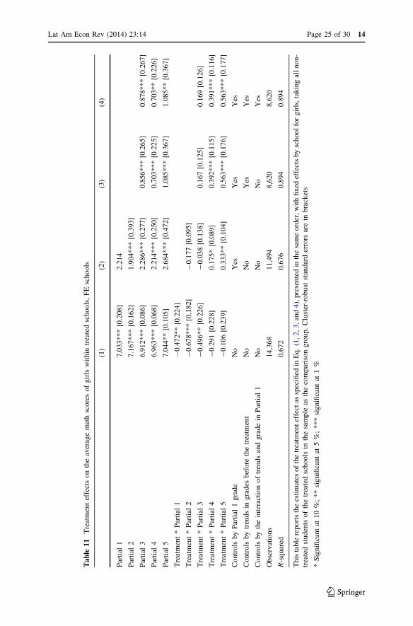
Ta
ble
11
Tre
atm
ent
effe
cts
on
the
aver
age
mat
hsc
ore
so
fg
irls
wit
hin
trea
ted
sch
oo
ls,
FE
sch
oo
ls
(1)
(2)
(3)
(4)
Par
tial
17
.03
3*
**
[0.2
08]
2.2
14
Par
tial
27
.16
7*
**
[0.1
62]
1.9
04
**
*[0
.39
3]
Par
tial
36
.91
2*
**
[0.0
86]
2.2
86
**
*[0
.27
7]
0.8
56
**
*[0
.26
5]
0.8
78
**
*[0
.26
7]
Par
tial
46
.96
3*
**
[0.0
68]
2.2
14
**
*[0
.25
0]
0.7
03
**
*[0
.22
5]
0.7
03
**
[0.2
26]
Par
tial
57
.04
4*
*[0
.10
5]
2.6
84
**
*[0
.47
2]
1.0
85
**
*[0
.36
7]
1.0
85
**
[0.3
67]
Tre
atm
ent
*P
arti
al1
-0
.472
**
[0.2
24]
Tre
atm
ent
*P
arti
al2
-0
.678
**
*[0
.18
2]
-0
.177
[0.0
95]
Tre
atm
ent
*P
arti
al3
-0
.496
**
[0.2
26]
-0
.038
[0.1
38]
0.1
67
[0.1
25]
0.1
69
[0.1
26]
Tre
atm
ent
*P
arti
al4
-0
.291
[0.2
28]
0.1
75
*[0
.08
9]
0.3
92
**
*[0
.11
5]
0.3
91
**
*[0
.11
6]
Tre
atm
ent
*P
arti
al5
-0
.106
[0.2
39]
0.3
33
**
[0.1
04]
0.5
63
**
*[0
.17
6]
0.5
63
**
*[0
.17
7]
Con
tro
lsb
yP
arti
al1
gra
de
No
Yes
Yes
Yes
Con
tro
lsb
ytr
end
sin
gra
des
bef
ore
the
trea
tmen
tN
oN
oY
esY
es
Con
tro
lsb
yth
ein
tera
ctio
no
ftr
end
san
dg
rad
ein
Par
tial
1N
oN
oN
oY
es
Ob
serv
atio
ns
14
,36
81
1,4
94
8,6
20
8,6
20
R-s
qu
ared
0.6
72
0.6
76
0.8
94
0.8
94
Th
ista
ble
rep
ort
sth
ees
tim
ates
of
the
trea
tmen
tef
fect
assp
ecifi
edin
Eq
.(1
,2,
3,
and
4),
pre
sen
ted
inth
esa
me
ord
er,
wit
hfi
xed
effe
cts
by
sch
ool
for
gir
ls,
tak
ing
all
no
n-
trea
ted
stud
ents
of
the
trea
ted
sch
oo
lsin
the
sam
ple
asth
eco
mp
aris
on
gro
up.
Clu
ster
-ro
bu
stst
and
ard
erro
rsar
ein
bra
cket
s
*S
ign
ifica
nt
at1
0%
;*
*si
gn
ifica
nt
at5
%;
**
*si
gn
ifica
nt
at1
%
Lat Am Econ Rev (2014) 23:14 Page 25 of 30 14
123

Table 13 shows a cost–benefit comparison with other programs aimed at
improving education in underdeveloped countries, including an estimate of the cost
effectiveness of the program analyzed in this paper. The remedial program analyzed
in this paper is more than eight times more cost effective than the teacher incentives
program evaluated by McEwan and Santibanez (2005), and four times less cost
effective than the remedial program evaluated by Banerjee et al. (2004).
8 Conclusions
This paper presents the results of the evaluation of a low-cost intervention in public
secondary schools in Mexico City, which consisted in offering free additional math
courses to students lagging behind their peers in marginalized low-income schools
in Mexico City.
We exploit the information available in all students’ (treated and not treated by
the program) transcripts enrolled in participating and non-participating schools.
Before the implementation of the program, participating students lagged behind
non-participating ones by more than half a base point in their GPA (over 10). As the
program was not randomly assigned, we suggest a difference-in-differences strategy
and, increasing the number of controls used, we discuss the validity of our method.
Regardless of the control variables included in the analysis, we find that students
participating in the program observed a higher increase in their school grades after
the implementation of the program, and that the difference in grades between the
two groups decreases over time. By the end of the school year (when the free extra
courses had been offered, on average, for 10 weeks), participating students’ grades
were not significantly lower than non-participating students’ grades. Nonetheless,
without any controls, the closing of the grade gap between treated and untreated
students seems to start before the program’s implementation. The differences in
scores before the implementation of the program between treated and non-treated
students remain significant when controlling for their grade in the first partial exam.
-0.8
-0.7
-0.6
-0.5
-0.4
-0.3
-0.2
-0.1
0
0.1
0.2
0.3
1 2 3 4 5
Diffs boys’ scores Diffs girls’ scores
Fig. 2 Differences between treated and untreated boys’ and girls’ scores
14 Page 26 of 30 Lat Am Econ Rev (2014) 23:14
123

Ta
ble
12
Tre
atm
ent
effe
cts
on
aver
age
mat
hst
andar
diz
edsc
ore
sw
ith
intr
eate
dsc
ho
ols
,F
Esc
ho
ols
(1)
(2)
(3)
(4)
Par
tial
10
.00
0[0
.08
8]
Par
tial
20
.00
4[0
.07
0]
0.0
01
[0.0
64
]
Par
tial
30
.00
3[0
.09
2]
0.0
00
[0.0
21
]-
0.0
01
[0.0
30]
0.0
01
[0.0
38]
Par
tial
40
.00
3[0
.08
4]
0.0
01
[0.0
24
]0
.000
[0.0
21]
-0
.002
[0.0
31]
Par
tial
50
.00
2[0
.02
4]
-0
.000
[0.0
02]
0.0
00
[0.0
30]
0.0
00
[0.0
17]
Tre
atm
ent
*P
arti
al1
-0
.379
**
*[0
.13
4]
Tre
atm
ent
*P
arti
al2
-0
.367
**
*[0
.09
9]
-0
.073
[0.0
55]
Tre
atm
ent
*P
arti
al3
-0
.186
*[0
.09
7]
0.0
47
[0.0
69
]0
.099
*[0
.05
2]
0.0
99
*[0
.05
3]
Tre
atm
ent
*P
arti
al4
-0
.046
[0.0
86]
0.1
71
**
[0.0
67]
0.2
14
**
*[0
.05
0]
0.2
13
**
*[0
.05
0]
Tre
atm
ent
*P
arti
al5
0.0
19
[0.0
81
]0
.21
8*
**
[0.0
68]
0.2
60
**
*[0
.05
4]
0.2
60
**
*[0
.05
5]
Con
tro
lsb
yP
arti
al1
gra
de
No
Yes
Yes
Yes
Con
tro
lsb
ytr
end
sin
gra
des
bef
ore
the
trea
tmen
tN
oN
oY
esY
es
Con
tro
lsb
yth
ein
tera
ctio
no
ftr
end
san
dg
rad
ein
Par
tial
1N
oN
oN
oY
es
Ob
serv
atio
ns
29
,62
52
3,7
00
17
,77
51
7,7
75
R-s
qu
ared
0.0
59
0.2
91
0.4
20
0.4
20
Th
ista
ble
rep
ort
sth
ees
tim
ates
of
the
trea
tmen
tef
fect
assp
ecifi
edin
Eq
.(1
,2,3,an
d4),
pre
sente
din
the
sam
eord
er,w
ith
fixed
effe
cts
by
school,
takin
gal
lth
enon-t
reat
ed
stu
den
tso
fth
etr
eate
dsc
ho
ols
com
par
ison
gro
up
.C
lust
er-r
ob
ust
stan
dar
der
rors
are
inb
rack
ets
*S
ign
ifica
nt
at1
0%
;*
*si
gn
ifica
nt
at5
%;
**
*si
gn
ifica
nt
at1
%
Lat Am Econ Rev (2014) 23:14 Page 27 of 30 14
123

Ta
ble
13
Cost
effe
ctiv
enes
san
alysi
sof
educa
tional
pro
gra
ms
Tre
atm
ent
Pla
ceG
rades
Du
rati
on
Imp
act
Co
stp
ers.
d.
Au
tho
rs
Cas
htr
ansf
ersa
Mex
ico
10
th-
5y
ears
0?
Ber
hm
anet
al.
(20
07)
Tea
cher
ince
nti
ves
Mex
ico
3rd
–6th
1y
ear
0.0
81
08
McE
wan
and
San
tib
anez
(20
05)
Com
pute
rsin
clas
sroom
saC
olo
mb
ia3
rd–
11
th2
yea
rs0
?B
arre
ra-O
sori
oan
dL
ind
en(2
00
9)
CA
RE
Sv
ou
cher
sC
olo
mb
ia6
th3
yea
rs0
.24
0A
ng
rist
etal
.(2
00
2)
Mat
htu
tori
ng
aM
exic
o9
th3
mo
nth
0.1
61
3.3
Gu
tier
rez
and
Ro
dri
go
(th
isp
aper
)
Rea
din
gtu
tori
ng
bC
hil
e4
th3
mo
nth
0.1
52
1.4
Cab
ezas
etal
.(2
01
1)
Tex
tbo
oks
Ken
ya
3rd
–8th
2y
ears
0?
Gle
ww
eet
al.
(20
02)
Rem
edia
lse
ssio
nsb
Ind
ia3
rd–
4th
1y
ear
0.1
43
.3B
aner
jee
etal
.(2
00
4)
Cam
era
mo
nit
ori
ng
bIn
dia
1st
–4
rd3
yea
rs0
.17
11
.7D
ufl
oet
al.
(20
12)
aIn
dic
ates
tho
sep
rog
ram
sw
her
eth
eo
utc
om
eo
bse
rved
was
am
ath
exam
bIn
dic
ates
that
the
ou
tco
me
ob
serv
edw
asa
read
ing
exam
.T
he
rest
loo
ks
atg
ener
alex
ams.
Th
eco
stis
in2
01
0U
Sd
oll
ars
14 Page 28 of 30 Lat Am Econ Rev (2014) 23:14
123

However, these differences disappear when including the information on students’
grades in the first two exams.
We then conclude that this paper shows evidence that interventions of this kind
can, at a relatively low cost, contribute to increase underperforming students’ exam
grades in the short run.
Acknowledgments We thank the Ministry of Education (SEP) in Mexico City for providing the data
and the Laboratory of Initiatives for Development (LID) for the commitment with the evaluation. We are
also grateful to Jere Behrman, Kensuke Teshima, and participants of the XVI meeting of the LACEA/
IADB/WB/UNDP Research Network on Inequality and Poverty (NIP) Conference for valuable comments
and suggestions. Emilio Gutierrez is grateful for support from the Asociacion Mexicana de Cultura.
Open Access This article is distributed under the terms of the Creative Commons Attribution License
which permits any use, distribution, and reproduction in any medium, provided the original author(s) and
the source are credited.
References
Almlund M, Lee A, Heckman J (2011) Personality psychology and economics. Handbook of economics
of education, chapter 1, vol 4
Angrist J, Bettinger E, Bloom E, King E, Kremer M (2002) Vouchers for private schooling in colombia:
evidence from a randomized natural experiment. Am Econ Rev 92(5):1535–1558
Banerjee A, Jacob S, Kremer M (2004) Promoting school participation in rural Rajasthan: results from
some prospective trials, MIT Department of Economics, Working paper
Banerjee A, Cole S, Duflo E, Linden L (2008) Remedying education: evidence from two randomized
experiments in India. Quart J Econ, MIT Press 122(3):1235–1264
Barham, Tania, Karen Macours, and John A. Maluccio (2013) ‘‘More Schooling and More Learnings?
Effects of a Three-Year Conditional Cash Transfer Program in Nicaragua after 10 years’’. IDB
Working Paper Series No. IDB-WP-432
Barrera-Osorio F, Linden LL (2009) The use and misuse of computers in education: evidence from a
randomized experiment in Colombia. World bank policy research working paper series, vol 2009
Behrman JR, Parker SW, Todd PE (2011) Do conditional cash transfers for schooling generate lasting
benefits? A five-year followup of PROGRESA/Oportunidades. J Hum Resour 46(1):93–122
Bowen William G, Chingos Mathew, McPherson Michael (2009) Test scores and high school grades as
predictors. Crossing the Finish Line: Completing College at America’s Public Universities’’.
Princeton University Press, Princeton, NJ, pp 112–133
Cabezas, Veronica, Jose I. Cuesta, and Francisco A. Gallego (2011) ‘‘Effects of Short Term Tutoring on
Cognitive and Non Cognitive Skills: Evidence from a Randomized Evaluation in Chile’’, Instituto de
Economıa, P. Universidad Catolica de Chile, Working paper
Chay Kenneth Y, McEwan Patrick J, Urquiola Miguel (2005) The central Role of Noise in Evaluating
Interventions that Use Test Scores to Rank Schools. Am Econ Rev 95(4):1237–1258
Duckworth AL, Quinn PD, Tsukayama E (2012) What no child left behind leaves behind: the roles of IQ
and self-control in predicting standardized achievement test scores and report card grades. J Educ
Psycol 104(2):439–451
Duflo Esther (2001) Schooling and labor market consequences of school construction in Indonesia:
evidence from an unusual policy experiment. Am Econ Rev Am Econ Assoc 91(4):795–813
Duflo E, Hanna R, Rya SP (2012) Incentives work: getting teachers to come to school. Am Econ Rev
102(4):1241–1278
Geiser S, Santelices MV (2007) Validity of high school grades in predicting student success beyond the
freshman year: high-school record VS. standardized tests as indicators of four-year college
outcomes. Center for Studies in Higher Education at the University of California, Berkeley CSHE
Glewwe P, Kremer M, Moulin S (2002) Textbooks and test scores: evidence from a prospective
evaluation in Kenya. BREAD Working Paper, Cambridge, MA
Lat Am Econ Rev (2014) 23:14 Page 29 of 30 14
123

INEE (2012) Panorama Educativo de Mexico 2012 Indicadores del Sistema Educativo Nacional. Mexico,
Instituto Nacional para la Evaluacion de la Educacion (INEE)
Jensen R (2010) The perceived returns to education and the demand for schooling. Q J Econ
125(2):515–548
Kremer M, Brannen C, Glennerster R (2013) The challenge of education and learning in the developing
world. Science 340:297–300
Kuncel NR, Hezlett SA (2007) Standardized tests predict graduate students’ success. Science
315:1080–1081
Lavy V, Schlosser A (2005) Targeted remedial education for underperforming teenagers: cost and
benefits. J Labor Econ XXIII:839–874
McEwan PJ, Santibanez L (2005) Teacher incentives and student achievement: evidence from a large-
scale reform in Mexico (unpublished paper)
Oliver PH, Guerin DW, Gottfried AW (2007) Temperamental task orientation: relation to high school and
college educational accomplishments. Learn Ind Differ 17(3):220–230
Sackett PR, Borneman MJ, Connelly BS (2008) High stakes testing in higher education and employment:
appraising the evidence for validity and fairness. Am Psychol 63(4):215–227
Willingham WW, Pollack JM, Lewis C (2002) Grades and test scores: accounting for observed
differences. J Educ Meas 39(1):1–37
14 Page 30 of 30 Lat Am Econ Rev (2014) 23:14
123