climate predictions of the twenty first century … · climate predictions of the twenty first...

International Journal of Scientific and Research Publications, Volume 4, Issue 7, July 2014 1 ISSN 2250-3153

www.ijsrp.org

Climate Predictions of the Twenty First Century Based

on Skill Selected Global Climate Models

J. Masanganise, T.W. Mapuwei, M. Magodora, C. Shonhiwa

Department of Physics and Mathematics, Bindura University of Science Education, P Bag 1020, Bindura, Zimbabwe

Abstract- A subset of global climate models from the Coupled

Model Inter-comparison Project 5 was used to explore the

changes in temperature and rainfall under moderate and high

climate change scenarios. We used downscaled model

projections of daily minimum and maximum temperature and

rainfall for the period 2040-2070 relative to the 1980-2010

reference period. Analysis of variance (ANOVA) was used to

test (at 5 % level of significance) for differences among the three

selected models in predicting the three variables under both

climate change scenarios. Where significant differences were

observed, we carried out multiple pair-wise comparison of the

models using Dunnett’s test. Overall, two of the three models

showed insignificant differences (p˂0.05) in predicting minimum

and maximum temperature while the other model deviated from

the two. However, we identified a consistent warming trend

across all the three models. The strength of global climate

models in rainfall prediction was found to lie in their ability to

simulate extremes, making the models relevant to sectors of the

economy that are vulnerable to extreme rainfall such as drought

and floods.

Index Terms- downscaled model projections, multiple pair-wise

comparison, extreme rainfall.

I. INTRODUCTION

variety of processes characterise the climate system. Some

of them include; boundary layer processes, radiative

processes and cloud processes. These processes interact with

each other both spatially and temporarily. Global climate models

(GCMs) have been shown to be useful tools for studying the

climate system (Pitman and Perkins, 2008; Houghton et al.,

2001; Randall et al., 2007), however because they have limited

resolutions at smaller scales, many climate processes are not

resolved adequately by climate models. Climate projections of

the future remain a challenge to many climate modeling

communities. Chiew et al. (2009) point out that climate change

impact assessment is likely to be more reliable if it is based on

future climate projections from the better GCMs. However, it is

difficult to objectively determine which GCMs are more likely to

give reliable future climate projections. Pitman and Perkins

(Pitman and Perkins, 2008) carried out climate projections for

Australia using GCMs. The authors based their study on the

assumption that a model that is able to simulate the probability

density function (PDF) of a climate variable well for the

twentieth century is likely to be able to simulate well the future

PDF of the same variable. Pitman and Perkins (2008) reported a

considerable overlap between the PDFs of the twentieth century

and those of the twenty first century. In this paper, we attempt to

provide climate projections of the twenty first century in

Zimbabwe, based on skill selected global climate models from

the Coupled Model Inter-comparison Project 5 (CMIP5). The

GCMs are based on the recently developed Representative

Concentration Pathway (RCP) emission scenarios. Measures of

model skill have been presented using a variety of metrics (e.g.

Johnson and Sharma, 2009; Carmen Sa´nchez de Cos, 2012;

Boberg et al., 2009; Perkins et al., 2007; Masanganise et al.,

2013). We follow the methodology of Masanganise et al.

(2014a) to select models that are highly skilful at simulating

daily probability density functions of maximum temperature

(Tmax), minimum temperature (Tmin) and rainfall (R). Masanganise

et al. (2014a) used probability density functions to compare daily

model simulations with daily observed climatology over the

same period. To rank the models, the authors used a match

metric method based on the common overlap of the model and

observed PDFs with a skill score value ranging from zero for no

overlap to a skill score of one for a perfect overlap. Using this

method, we select three models that best match observations for

each variable out of ten models and apply them to make climate

projections of the mid-century (2040-2070) period relative to the

1980-2010 baseline period. The projections are based on the

moderate (RCP4.5) emission scenario and the highest (RCP8.5)

emission scenario. The methodology is provided in section 2,

results and discussion in section 3 and lastly, conclusions in

section 4.

II. DATA AND METHODOLOGY

The study was carried out in Zimbabwe in a district called

Mutoko. The climatic variables used were maximum air

temperature Tmax, minimum air temperature Tmin and rainfall R.

The choice of these three variables was partly based on data

availability. Details of data acquisition and processing are

presented in Masanganise et al. (2014a). The GCMs used are

listed in Table l.

A

http://ijsrp.org/

International Journal of Scientific and Research Publications, Volume 4, Issue 7, July 2014

2 ISSN 2250-3153

www.ijsrp.org

Table 1 A list of the 10 coupled global climate models from which 3 models were selected.

Model name Modeling centre(or group) Resolution (degrees)

latitude x longitude

Beijing Normal University Earth

System model (BNU-ESM)

College of Global Change and Earth System

Science, Beijing Normal University, China

2.810 x 2.810

Canadian Earth System Model

version 2 (CanESM2)

Canadian Centre for Climate Modelling and

Analysis, Canada

2.810 x 2.810

Centre National de Recherche

Météorologiques Climate Model

version 5 (CNRM-CM5)

CNRM/Centre Europeen de Recherche et

Formation Avancees en Calcul Scientifique,

France Calcul Scientifique, France

1.410 x 1.410

Flexible Global Ocean-

Atmosphere-Land System

Modelspectral version 2

(FGOALS-s2)

State Key Laboratory of Numerical Modeling

for Atmospheric Sciences and Geophysical

Fluid Dynamics, Institute of Atmospheric

Physics, Chinese Academy of Sciences, China

1.670 x 2.810

Geophysical Fluid Dynamics

Laboratory Earth System Model

(GFDL-ESM2G)

NOAA Geophysical Fluid Dynamics

Laboratory

2.000 x 2.500

Geophysical Fluid Dynamics

Laboratory Earth System Model

(GFDL-ESM2M)

NOAA Geophysical Fluid Dynamics

Laboratory

2.000 x 2.500

Model for Interdisciplinary

Research on Climate-Earth

System, version 5 (MIROC5)

The University of Tokyo, National Institute for

Environmental Studies and Japan Agency for

Marine-Earth Science and Technology

1.417 x 1.406

Atmospheric Chemistry Coupled

Version of Model for

Interdisciplinary Research on

Climate-Earth System (MIROC-

ESM-CHEM)

Japan Agency for Marine-Earth Science and

Technology, The University of Tokyo and

National Institute for Environmental Studies

2.857 x 2.813

Model for Interdisciplinary

Research on Climate-Earth

System (MIROC-ESM)

Japan Agency for Marine–Earth Science and

Technology, The University of Tokyo and

National Institute for Environmental Studies

2.857 x 2.813

Meteorological Research Institute

Coupled General Circulation

Model version 3 (MRI-CGCM3)

Meteorological Research Institute, Japan 1.132 x 1.125

Three models were selected from Table 1

using the match metric method described in

Masanganise et al. (2014a). For temperature, these

were models that were able to capture at least 97 %

of the observed probability density function in their

simulations. In the case of rainfall, the skill scores

were low and we selected only those models that

were able to capture at least 31 % of the observed

probability density function. We then analysed

climate projections for the period 2040-2070

relative to the 1980-2010 baseline based on the

three global climate models selected from Table 1.

i. Temperature and rainfall projections

Using downscaled historical (1980-2010)

daily data, we calculated monthly mean values for

Tmax, Tmin and R for each climate change scenario.

We also calculated monthly mean values for the

same variables and scenarios using projections for

the period 2040-2070. Anomalies were then

calculated as the absolute difference (2040-2070)

minus (1980-2010) for each model and variable to

depict the magnitude of change.

ii. Model convergence

Model convergence was assessed using

probability density functions (PDFs) to establish

the consistency in predictions from the 3 models.

We calculated PDFs for each of the variables Tmax,

Tmin and R using downscaled GCM projections for

the period 2040-2070 under RCP4.5 and RCP8.5.

The PDFs were constructed using the method

described in Masanganise et al. (2014a). Analysis

of variance (ANOVA) was used to test (at 5 %

level of significance) for differences among the

three selected models in predicting Tmax, Tmin and R

under both climate change scenarios. If the

differences were observed to be significant under

ANOVA, we proceeded to carry out multiple pair-

wise comparison of the models using Dunnett’s

test.

III. RESULTS AND DISCUSSION

i. Projections of temperature

Monthly time series plots of temperature

anomalies are shown in Figure 3.1 to Figure 3.4

http://ijsrp.org/


3 ISSN 2250-3153

www.ijsrp.org

Figure 3.1 Projections of mean monthly anomalies for Tmin for the period 2040-2070 under RCP4.5

Figure 3.2 Projections of mean monthly anomalies for Tmax for the period 2040-2070 under RCP4.5

http://ijsrp.org/


4 ISSN 2250-3153

www.ijsrp.org

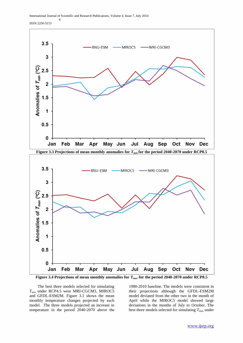
Figure 3.3 Projections of mean monthly anomalies for Tmin for the period 2040-2070 under RCP8.5

Figure 3.4 Projections of mean monthly anomalies for Tmax for the period 2040-2070 under RCP8.5

The best three models selected for simulating

Tmin under RCP4.5 were MRI-CGCM3, MIROC5

and GFDL-ESM2M. Figure 3.1 shows the mean

monthly temperature changes projected by each

model. The three models projected an increase in

temperature in the period 2040-2070 above the

1980-2010 baseline. The models were consistent in

their projections although the GFDL-ESM2M

model deviated from the other two in the month of

April while the MIROC5 model showed large

deviations in the months of July to October. The

best three models selected for simulating Tmax under

http://ijsrp.org/


5 ISSN 2250-3153

www.ijsrp.org

RCP4.5 were CanESM2, BNU-ESM and MIROC-

ESM-CHEM. Temperature projections by these

models are less than about 1 °C in most of the

months as shown in Figure 3.2. Under RCP8.5, the

models selected for simulating Tmin were MRI-

CGCM3, MIROC5 and BNU-ESM. The same

models were also selected for simulating Tmax.

These models projected a consistent warming trend

of about 1 °C or less as shown in Figure 3.3 and

Figure 3.4. Time series plots of Figure 3.3 and

Figure 3.4 indicate very similar trends predicted by

the MRI-CGCM3 and MIROC5 models. By using

fewer models, we found a reduction in the

amplitude of warming compared to that reported in

Masanganise et al. (2014b) who applied all the 10

climate models to make climate projections over

the same period.

ii. Projections of rainfall

Monthly time series plots of rainfall anomalies

are shown in Figure 3.5 and Figure 3.6

Figure 3.5 Projections of mean monthly anomalies for R for the period 2040-2070 under RCP4.5

http://ijsrp.org/


6 ISSN 2250-3153

www.ijsrp.org

Figure 3.6 Projections of mean monthly anomalies for R for the period 2040-2070 under RCP8.5

The best three models selected for simulating

R under RCP4.5 were GFDL-ESM2G, GFDL-

ESM2M and MRI-CGCM3. The same models were

also selected for simulating R under RCP8.5.

Figure 3.5 and Figure 3.6 show the mean monthly

rainfall change projections by the three models.

There was a wide variation in the predictions by the

three models mainly in the months of January-April

where the spread of rainfall change projections is

large. However, the three models agreed in the

direction of rainfall change in the months of

October-December under both climate change

scenarios supporting findings by Masanganise et al.

(2014b)

iii. Analysis of PDFs for Tmin and Tmax

PDFs are shown in Figure 3.7 to Figure 3.10

http://ijsrp.org/


7 ISSN 2250-3153

www.ijsrp.org

Figure 3.7 Probability density functions of the three models for Tmin for the period 2040-2070 under

RCP4.5

Figure 3.8 Probability density functions of the three models for Tmax for the period 2040-2070 under

RCP4.5

http://ijsrp.org/


8 ISSN 2250-3153

www.ijsrp.org

Figure 3.9 Probability density functions of the three models for Tmin for the period 2040-2070 under

RCP8.5

Figure 3.10 Probability density functions of the three models for Tmax for the period 2040-2070 under

RCP8.5

Figure 3.7 to Figure 3.10 show the PDFs for

Tmin and Tmax for each climate change scenario.

Overall, the shapes of the PDFs are in agreement

with each other, an indication that the 3 models

predicted similar trends. In Figure 3.9 and Figure

3.10, PDFs for the MIROC5 and MRI-CGCM3 are

http://ijsrp.org/


9 ISSN 2250-3153

www.ijsrp.org

almost overlapping. This is in agreement with time

series plots in Figure 3.3 and Figure 3.4. In general,

there was an increase in the amount of overlap of

the PDFs when three best models were used as

compared to the amount of overlap reported in

Masanganise et al. (2014b) in which all the 10

models were used.

iv. Analysis of PDFs for R

PDFs are shown in Figure 3.11 and Figure

3.12

Figure 3.11 Probability density functions of the three models for R for the period 2040-2070 under

RCP4.5

Figure 3.12 Probability density functions of the three models for R for the period 2040-2070 under

RCP8.5

http://ijsrp.org/


10 ISSN 2250-3153

www.ijsrp.org

Figure 3.11 and Figure 3.12 show the PDFs for R

for the two climate change scenarios. Models tend

to agree at the extremes of the distribution as

shown by the PDFs clustering in these regions. In

between the extremes, PDFs are widely separated

indicating some level of disagreement in

predictions. Rainfall is difficult to predict than

temperature (Pitman and Perkins, 2008) and it is

expected that there would be considerable

uncertainty in the projections of rainfall using

climate models.

v. Analysis of variance (ANOVA) and

multiple pair wise comparison.

Table 2 Analysis of variance for predicting Tmin under RCP4.5

Sum of Squares df Mean Square F Sig.

Between Groups 899.278 2 449.639 28.354 .000

Within Groups 538634.433 33966 15.858

Total 539533.711 33968

We found significant differences (p˂0.05)

among the three models in predicting Tmin. The test

statistics are shown in Table 2. We then carried out

multiple pair wise comparison.

Table 3 Multiple pair wise comparison of the three models for predicting Tmin under RCP4.5

I-Model J-Model

Mean Difference

(I-J) Std. Error Sig.

95% Confidence Interval

Lower

Bound Upper Bound

GFDL-ESM2M MIROC5 .118 .054 .080 .00 .24

MRI-CGCM3 .389* .053 .000 .26 .51

MIROC5 GFDL-ESM2M -.118 .054 .080 -.24 .01

MRI-CGCM3 .271* .052 .000 .15 .40

MRI-CGCM3 GFDL-ESM2M -.389* .053 .000 -.51 -.26

MIROC5 -.271* .052 .000 -.40 -.15

*. The mean difference is significant at the 0.05 level.

The statistics in Table 3 showed significant

differences (p˂0.05) between MRI-CGCM3 and

GFDL-ESM2M models. The models MIROC5 and

MRI-CGCM3 were also significantly different

(p˂0.05). However, no significant differences were

observed between the MIROC5 and the GFDL-

ESM2M model (p>0.05). Also see Figure 3.7 for

pictorial differences. The MRI-CGCM3 model may

be excluded in predicting minimum temperature

under RCP4.5.

Table 4 Analysis of variance for predicting Tmax under RCP4.5


Between Groups 6026.939 2 3013.470 235.897 .000

Within Groups 433899.301 33966 12.775

Total 439926.240 33968

There were significant differences (p˂0.05) among the three models in predicting Tmax under

RCP4.5 as shown in Table 4.

Table 5 Multiple pair wise comparison of the three models for predicting Tmax under RCP4.5

I-Model J-Model

Mean Difference


95% Confidence Interval

Lower

Bound Upper Bound

BNU-ESM CanESM2 -.682* .048 .000 -.80 -.57

http://ijsrp.org/


11 ISSN 2250-3153

www.ijsrp.org

MIROC-ESM-

CHEM

-1.012* .047 .000 -1.12 -.90

CanESM2 BNU-ESM .682* .048 .000 .57 .80

MIROC-ESM-

CHEM

-.330* .047 .000 -.44 -.22

MIROC-ESM-

CHEM

BNU-ESM 1.012* .047 .000 .90 1.12

CanESM2 .330* .047 .000 .22 .44


Multiple pair wise comparison showed

significant differences (p˂0.05) between all of the

three possible pairs as shown in Table 5. The

amount of overlap in Figure 3.8 also supports this.

If the models are to be used for making predictions,

they have to be applied independently.

Table 6 Analysis of variance for predicting Tmin and Tmax under RCP8.5


Tmin Between Groups 1936.562 2 968.281 60.837 .000

Within Groups 540600.027 33966 15.916

Total 542536.589 33968

Tmax Between Groups 1543.572 2 771.786 61.179 .000

Within Groups 428484.739 33966 12.615

Total 430028.311 33968

Significant differences (p˂0.05) were obtained

among the three models in predicting both Tmin and

Tmax under RCP8.5. The test statistics are shown in

Table 6.

Table 7 Multiple pair wise comparison of the three models for predicting Tmin and Tmax under RCP8.5

Dependent

Variable I-Model J-Model

Mean

Difference


95% Confidence

Interval

Lower

Bound

Upper

Bound

Tmin BNU-ESM MIROC5 .482* .054 .000 .35 .61

MRI-CGCM3 .528* .053 .000 .40 .65

MIROC5 BNU-ESM -.482* .054 .000 -.61 -.35

MRI-CGCM3 .046 .052 .764 -.08 .17

MRI-CGCM3 BNU-ESM -.528* .053 .000 -.65 -.40

MIROC5 -.046 .052 .764 -.17 .08

Tmax BNU-ESM MIROC5 .456* .048 .000 .34 .57

MRI-CGCM3 .449* .048 .000 .34 .56

MIROC5 BNU-ESM -.456* .048 .000 -.57 -.34

MRI-CGCM3 -.007 .046 .998 -.12 .10

MRI-CGCM3 BNU-ESM -.449* .048 .000 -.56 -.34

MIROC5 .007 .046 .998 -.10 .12


Multiple pair wise comparison showed that

there were significant differences (p˂0.05) in the

prediction of Tmin by the BNU-ESM and MIROC5

models as shown in Table 7. Similar results were

obtained for the BNU-ESM and MRI-CGCM3

models. However, no significant differences

(p>0.05) were observed between the MIROC5 and

the MRI-CGCM3 models. This is in agreement

with the results shown in Figure 3.9. The same

trend was observed in the prediction of Tmax by the

three models as shown in Table 7 (also see Figure

http://ijsrp.org/


12 ISSN 2250-3153

www.ijsrp.org

3.10). The BNU-ESM model may be excluded in predicting both Tmin and Tmax under RCP8.5.

Table 8 Analysis of variance for predicting R under RCP4.5


Between Groups 401.948 2 200.974 3.087 .051

Within Groups 2211533.046 33966 65.110

Total 2211934.994 33968

The three models were not significantly

different (p>0.05) in predicting rainfall under

RCP4.5. The three models GFDL-ESM2G, MRI-

CGCM3 and GFDL-ESM2M may be used

concurrently.

Table 9 Analysis of variance for predicting R under RCP8.5


Between Groups 764.560 2 382.280 6.261 .002

Within Groups 2073592.791 33964 61.053

Total 2074357.351 33966

The three models were significantly different

(p˂0.05) in predicting rainfall under RCP8.5.

Table 10 Multiple pair wise comparison of the three models for predicting R under RCP8.5

I-Model J-Model

Mean Difference


95% Confidence

Interval

Lower

Bound

Upper

Bound

GFDL-ESM2G GFDL-ESM2M .18910 .10616 .206 -.0622 .4405

MRI-CGCM3 .36745* .10403 .000 .1213 .6136

GFDL-ESM2M GFDL-ESM2G -.18910 .10616 .206 -.4405 .0622

MRI-CGCM3 .17834 .10130 .215 -.0615 .4182

MRI-CGCM3 GFDL-ESM2G -.36745* .10403 .000 -.6136 -.1213

GFDL-ESM2M -.17834 .10130 .215 -.4182 .0615


Multiple pair wise comparison indicated

significant differences (p˂0.05) between the

GFDL-ESM2G and MRI-CGCM3 models under

the RCP8.5. The GFDL-ESM2G and GFDL-

ESM2M models were not significantly different

(p>0.05). Similarly, the GFDL-ESM2M and the

MRI-CGCM3 models were not significantly

different (p>0.05) in predicting rainfall under

RCP8.5. Linking statistical results and PDFs in

Figure 3.12, the GFDL-ESM2G model predicts

higher values of rainfall; MRI-CGCM3 predicts

low values of rainfall while GFDL-ESM2M

predicts moderate values. We recommend the use

of the three models to allow for comparison of

predictions. Table 11 is a summary of the selected

models under different RCPs.

http://ijsrp.org/

International Journal of Scientific and Research Publications, Volume 4, Issue 7, July 2014 13

ISSN 2250-3153

www.ijsrp.org

Table 11 Summary of selected models

Climatic variable Selected models Comment

RCP4.5

Minimum temperature MIROC5 and GFDL-ESM2M MRI-CGCM3 excluded

Maximum temperature BNU-ESM, CanESM2 and MIROC-ESM-CHEM

All models predicted differently

Rainfall GFDL-ESM2G, MRI-CGCM3 and GFDL-ESM2M

No significant differences

RCP8.5

Minimum temperature MIROC5 and MRI-CGCM3 BNU-ESM excluded

Maximum temperature MIROC5 and MRI-CGCM3 BNU-ESM excluded

Rainfall GFDL-ESM2G, GFDL-ESM2M and MRI-CGCM3

High, moderate and low predictors respectively

IV. CONCLUSIONS

Climate projections of the mid-century were analysed using

a subset of global climate models from the Coupled Model Inter-

comparison Project 5. The projections were based on moderate

and high climate change scenarios. All the three models used

projected a rise in temperature by about 1 °C in the period 2040-

2070 relative to the 1980-2010 reference period. However, in

some cases, some models were excluded because they predicted

differently. The three models used to simulate rainfall change

were found to be consistent in simulating extremes. We therefore

recommend that such models be used by sectors that are

vulnerable to extreme rainfall such as drought and floods.

REFERENCES

[1] Boberg, F., Berg, P., Thejll, P., Gutowski, W. J. and Christensen, J. H. 2009. Improved confidence in climate change projections of precipitation further evaluated using daily statistics from ENSEMBLES models. Climate Dynamics 35:1509-1520. doi 10.1007/s00382-009-0683-8.

[2] Carmen Sańchez de Cos, C., Sańchez-Laulhe´, J.M., Jimeńez-Alonso, C., Sancho-Avila, J.M. and Rodriguez-Camino, E. 2013. Physically based evaluation of climate models over the Iberian Peninsula. Climate Dynamics 40:1969-1984 DOI 10.1007/s00382-012-1619-2.

[3] Chiew, F.H.S., Kirono, D.G.C., Kent, D. and Vaze, J. 2009. Assessment of rainfall simulations from global climate models and implications for climate change impact on runoff studies. 18th World IMACS / MODSIM Congress, Cairns, Australia. http://mssanz.org.au/modsim09. (Last accessed 26/06/2013).

[4] Houghton, J. T., Ding, Y., Griggs, D. J., Noger, M., van der Linden, P. J., Dai, X., Maskell, K. and Johnson, C. A. Eds. 2001. Climate Change 2001: The Scientific Basis. Cambridge University Press, 881 pp.

[5] Johnson, F. and Sharma, A. 2009. Measurement of GCM Skill in Predicting Variables Relevant for Hydroclimatological Assessments. Journal of Climate 22: 4373-4382.

[6] Masanganise, J., Magodora, M., Mapuwei, T. and Basira, K. 2014a. An assessment of CMIP5 global climate model performance using probability

density functions and a match metric method. Science Insights: An International Journal 4(1): 1-8.

[7] Masanganise, J., Mapuwei, T.W., Magodora, M. and Basira, K. 2014b. Multi-Model Projections of Temperature and Rainfall under Representative Concentration Pathways in Zimbabwe. International Journal of Science and Technology 3(4): 229-240.

[8] Masanganise, J., Chipindu, B., Mhizha, T., Mashonjowa, E. and Basira, K. 2013. An evaluation of the performances of Global Climate

[9] Models (GCMs) for predicting temperature and rainfall in Zimbabwe. International Journal of Scientific and Research Publications 3:1-11.

[10] Perkins, S. E., Pitman, A. J., Holbrook, N. J. and Mcaneney, J. 2007. Evaluation of the AR4 Climate Models’ Simulated Daily Maximum

[11] Temperature, Minimum Temperature, and Precipitation over Australia Using Probability Density Functions. Journal of Climate 20: 4356-4376.

[12] Pitman, A. J. and Perkins, S. E. 2008. Regional Projections of Future Seasonal and Annual Changes in Rainfall and Temperature over

[13] Australia Based on Skill-Selected AR4 Models. Earth Interactions 12: 1-50. doi: http://dx.doi.org/10.1175/2008EI260.1.

[14] Randall, D. A. and Co-authors. 2007. Climate models and their evaluation. Climate Change 2007: The Physical Science Basis, S. Solomon et al., Eds., Cambridge University Press, 589-662.

AUTHORS

First Author – J. Masanganise, Department of Physics and

Mathematics, Bindura University of Science Education, P Bag

1020, Bindura, Zimbabwe, E-mail: [email protected]

Second Author – T.W. Mapuwei, Department of Physics and


1020, Bindura, Zimbabwe

Third Author – M. Magodora, Department of Physics and



Fourth Author – C. Shonhiwa, Department of Physics and



http://ijsrp.org/

climate predictions of the twenty first century … · climate predictions of the twenty first...

Documents