CLIMATE RESEARCHClim Res

Vol. 59: 1–13, 2014doi: 10.3354/cr01204

Published February 4

1. INTRODUCTION

Climate monitoring is mostly based either directlyon station measurements of climate characteristics(surface air temperature, precipitation, cloud cover,etc.), or on some post-processed form of those meas-urements, such as gridded datasets. The analysis ofclimate patterns can be performed for each indi -vidual climate variable separately, or the data canbe aggregated, for example, by using some kind of climate classification that integrates several climatecharacteristics. These classifications usually corre-spond to vegetation distribution in the sense thateach climate type is dominated by one vegetationzone or eco-region (Köppen, 1936, Trewartha & Horn1980, Bailey 2009, Baker et al. 2010). Thus, climateclassifications can also represent a convenient, i.e.integrated, but still quite simple tool for the valida-tion of climate models and for the analysis of simu-lated future climate changes.

The first quantitative classification of Earth’s cli-mate was developed by Wladimir Köppen in 1900(Kottek et al. 2006). Even though various differentclassifications have been developed since then, thosebased on Köppen’s original approach (Köppen 1923,1931, 1936) and its modifications are still among themost frequently used systems. For application to climate model outputs the Köppen-Geiger system(Köppen 1936, Geiger 1954) or Köppen-Trewarthamodification (e.g. Trewartha & Horn 1980) are usu-ally utilized.

The first digital Köppen-Geiger world map for thesecond half of 20th century was published by Kotteket al. (2006). This study used the Climatic ResearchUnit (CRU) TS2.1 dataset (Mitchell & Jones 2005) andthe VASClim0v1.1 precipitation data (gpcc.dwd.de)for the period of 1951−2000. Prior to this, many text-books reproduced a copy of one of the historicalhand-drawn maps from Köppen (1923, 1931 or 1936)or Geiger (1961). Following up on the work of Kottek

© Inter-Research 2014 · www.int-res.com*Corresponding author: Michal.Belda@mff.cuni.cz

Climate classification revisited: from Köppen toTrewartha

Michal Belda*, Eva Holtanová, Tomáš Halenka, Jaroslava Kalvová

Charles University in Prague, Dept. of Meteorology and Environment Protection, 18200 Prague, Czech Republic

ABSTRACT: The analysis of climate patterns can be performed separately for each climatic vari-able or the data can be aggregated, for example, by using a climate classification. These classifi-cations usually correspond to vegetation distribution, in the sense that each climate type is domi-nated by one vegetation zone or eco-region. Thus, climatic classifications also represent a con -venient tool for the validation of climate models and for the analysis of simulated future climatechanges. Basic concepts are presented by applying climate classification to the global ClimateResearch Unit (CRU) TS 3.1 global dataset. We focus on definitions of climate types according tothe Köppen-Trewartha climate classification (KTC) with special attention given to the distinctionbetween wet and dry climates. The distribution of KTC types is compared with the original Köp-pen classification (KCC) for the period 1961−1990. In addition, we provide an analysis of the timedevelopment of the distribution of KTC types throughout the 20th century. There are observablechanges identified in some subtypes, especially semi-arid, savanna and tundra.

KEY WORDS: Köppen-Trewartha · Köppen · Climate classification · Observed climate change ·CRU TS 3.10.01 dataset · Patton’s dryness criteria

Resale or republication not permitted without written consent of the publisher

FREEREE ACCESSCCESS

Clim Res 59: 1–13, 2014

et al. (2006), Rubel & Kottek (2010) produced a seriesof digital world maps covering the extended period1901−2100. These maps are based on CRU TS2.1 andon GPCC Version 4 data, and Global Climate Model(GCM) outputs for the period 2003−2100 were takenfrom the TYN SC 2.0 dataset (Mitchell et al. 2004). Anew high-resolution global map of the Köppen-Geiger classification was produced by Peel et al.(2007). Climatic variables used for the determinationof climate types were calculated using data from4279 stations of the Global Historical ClimatologyNetwork (Peterson & Vose 1997) and interpolatedonto a 0.1° × 0.1° grid.

One of the first attempts to use the Köppen climateclassification (KCC) to validate GCM outputs waspresented by Lohmann et al. (1993). The observedclimate conditions were represented by temperaturedata from Jones et al. (1991) and precipitation datafrom Legates & Willmott (1990). In Kalvová et al.(2003), the KCC was applied to CRU gridded climato -logy (New et al. 1999) for the periods 1961−1990 and1901−1921. The latter period was used for compari-son with the original results described by Köppen(1931).

The modifications of KCC proposed by G. T. Tre-wartha (Trewartha 1968, Trewartha & Horn 1980) adjust both the original temperature criteria and thethresholds separating wet and dry climates (fordetails see Section 3). The resulting classification isusually denoted the Köppen-Trewartha classification(KTC). Fraedrich et al. (2001) applied KTC to CRUdata (New & Hulme 1998) with 0.5° × 0.5° resolution(excluding Antarctica). They analyzed the shifts ofclimate types during the 20th century in relation tochanges in circulation indices (Pacific Decadal Oscil-lation and North Atlantic Oscillation). KTC typeswere also used by Guetter & Kutzbach (1990), whostudied atmo spheric general circulation model simu-lations of the last interglacial and glacial climates(126 and 18 thousand yr before present). Further-more, Baker et al. (2010) compared KTC types overChina for historical (1961−1990) and projected futureclimates (2041− 2070) simulated using the HadCM3model under the SRES A1F1 scenario (Nakicenovic &Swart 2000). The KTC types were obtained by apply-ing classification criteria for each grid box of the 30 yrPRISM climato logy (Daly et al. 2002) and to eco-regions defined through the Multivariate Spatio-Temporal Clustering algorithm. Feng et al. (2012)used the KTC to evaluate climate changes and theirimpact on vegetation for the area north of 50° N andthe period 1900−2099, focusing on the Arctic region.In addition to the observed data, the outputs of 16

AR4 GCMs (Meehl et al. 2007) under SRES scenariosB1, A1B, and A2 were used. De Castro et al. (2007)used the KTC for validation of 9 regional climatemodels (RCMs) from project PRUDENCE (http://prudence.dmi.dk) over Europe for the period 1961−1990 and for the analysis of simulated climate changefor 2071−2100 under scenario SRES A2. They usedthe CRU climatology as the observed dataset (New etal. 1999). Wang & Overland (2004) quantified histori-cal changes in vegetation cover in the Arctic (1900−2000) by applying the KTC to NCEP/ NCAR reanaly-sis (Kalnay et al. 1996) and CRU TS2.0 (New et al.1999, 2000), and compared the results with satelliteNDVI (Normalized Difference Vegetation Index, pro-viding an areal average measure of the amount ofvegetation and its photosynthetic activity). Gersten-garbe & Werner (2009) studied how global warmingin the period 1901−2003 influenced Europe by usingthe KTC types. Their results are based on the datawith spatial resolution of 0.5° × 0.5° produced at thePotsdam Institute for Climate Impact Research.

The above examples of studies employing climateclassifications show how different authors use vari-ous datasets with diverse spatial resolution for timeperiods of different lengths (e.g. 15, 30, or 50 yr) andover various geographical areas and spatial scales.However, it is not always clearly described how theclimate types are defined and which modification ofthe respective climate classification is used. There-fore, it is appropriate to describe KTC in detail, itsdifferences from KCC, and to create new maps of theKTC types based on the latest version of the CRUdataset; these are the goals of the present study.These results will provide background for furthervalidation of the new generation of CMIP5 GCMs(Taylor et al. 2012), analysis of recent climate change,and for the evaluation of simulated future climatechange. These topics will be addressed in studies weare currently preparing for publication.

This study includes only a part of the graphicalmaterials used for our analysis. Additional maps andgraphs can be found on a supplementary website athttp://kmop.mff.cuni.cz/ projects/ trewartha.

2. DATA

As an observational data source we use the CRUTS 3.10.01 dataset (Harris et al. in press). CRU TS3.10provides a monthly time-series of global gridded databased on observations from more than 4000 stations.Among other variables, it includes the mean surfaceair temperature and precipitation, on which the cli-

2

Belda et al.: Climate classification

mate classifications used in this work are based. CRUTS3.10 is available over land areas excluding Antarc-tica at a high spatial resolution of 0.5° × 0.5° and cov-ers the period 1901−2009. We concentrate on theperiod 1901−2005, which is also used in further stud-ies for the validation of GCMs. The version 3.10.01was the most recent update of the dataset at the timeof undertaking this analysis. This update includescorrections to precipitation data, as well as to thedata files of wet days and frost frequency.

3. KOPPEN-TREWARTHA CLIMATE CLASSIFICATION SCHEME

In the present paper, we adopt the KTC defined inTrewartha & Horn (1980) with Patton’s boundaries ofarid climates (Patton 1962). This scheme builds uponthe original Köppen system and introduces variousadjustments to make the climate types better corre-spond with the observed boundaries of natural land-scapes (de Castro et al. 2007). Some of the modifica-tions introduced by the KTC also deal with a certainvagueness of the KCC formulations. This section willdescribe the KTC and compare the definitions withthe KCC, as described by Köppen (1936). See Table 1and Table 3 for respective summaries of the KTC andKCC classifications.

The KTC defines 6 main climatic groups. Five ofthem (denoted as A, C, D, E, and F) are basic thermalzones. The sixth group B is the dry climatic zone thatcuts across the other climate types, except for thepolar climate F. The main climate types are, similarlyto those of the KCC, determined according to thelong-term annual and monthly means of surface airtemperature and amounts of precipitation. The mainmodifications in the KTC in comparison with theKCC are the different definitions of groups C and D,a newly defined E type, and different thresholds fordistinguishing between wet and dry climates. In thefollowing text, the individual climate types will bediscussed in detail.

3.1. Group A: tropical humid climates

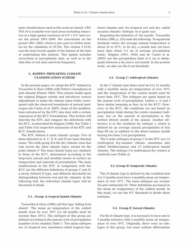
Trewartha & Horn (1980) call this type ‘killing frostabsent’. The mean air temperature of the coldestmonth must be over 18°C (i.e all months must bewarmer than 18°C). The subtypes of this group aredefined according to the annual cycle of precipitation(number of dry months) Table 1. Two main subtypesare Ar (tropical wet, sometimes called tropical rain-

forest climate) and Aw (tropical wet and dry, calledsavanna climate). Subtype As is quite rare.

Regarding the definition of ‘dry month’, Trewartha& Horn (1980, p. 235) state the following: ‘In equa toriallowlands where the average annual temperature isabout 25 to 27°C, to be dry, a month may not havemore than about 5.5 cm of average precipitationtotals.’ Köppen (1931, 1936) and de Castro et al.(2007) use the precipitation limit of 6 cm to distin-guish between a dry and a wet month. In the presentstudy, we also use the 6 cm threshold.

3.2. Group C : subtropical climates

In the C climate type there must be 8 to 12 monthswith a monthly mean air temperature of over 10°Cand the temperature of the coolest month must belower than 18°C. The subtypes are again based onthe annual cycle of precipitation. Letters s, w and fhave similar meaning as they do in the KCC. How-ever, in the KCC, the conditions are not based onprecipitation totals during the winter (summer) half-year, but on the amount of precipitation in thewettest (driest) month of the season. Another dif -ference is in the condition for subtype s, which isdefined by an average annual precipitation of lessthan 89 cm, in addition to the driest summer monthhaving less than 3 cm precipitation.

The 2 main subtypes of group C in the KTC are Cs(subtropical dry-summer climate, sometimes alsocalled Mediterranean) and Cf (subtropical humid climate). The subtype Cw (subtropical dry-winter) isrelatively rare (Table 2).

3.3. Group D : temperate climates

The D climate type is defined by the condition that4 to 7 months must have a monthly mean air temper-ature of over 10°C. The main subtypes are oceanicDo and continental Dc. Their definitions are based onthe mean air temperature of the coldest month. Inthis study, we use the 0°C threshold to divide thesesubtypes.

3.4. Group E : boreal climates

For the E climate type, it is necessary to have one to3 months inclusive with a monthly mean air temper-ature of over 10°C. Originally, there were no sub-types of this group, but some authors differentiate

3

Clim Res 59: 1–13, 2014

oceanic and continental subtypes in the same way asin type D (e.g. de Castro et al. 2007). This distinctioncan prove useful especially when dealing with spe-cific regional features. For the purposes of globalevaluation we use the original definition that doesnot divide the E type. The KCC does not have ananalogous climate group.

3.5. Group F : polar climates

Within the F type, all months must have a monthlymean air temperature of below 10°C. The subtypesare Ft (tundra) with the warmest month’s air tem -perature above 0°C and Fi (ice cap) where the airtemperature in all months remains below 0°C.

3.6. Group B: dry climates

One of the main differences between the KCC andthe KTC is the definition of dry climates B, or moreprecisely, the formula for the calculation of the dry-ness threshold used in these definitions. In the KCC,the boundary distinguishing between wet and dryclimates is defined according to Eq. (1), which differsaccording to the annual precipitation pattern:

R = 2T + 14 for evenly distributed rainfall (1)R = 2T for rainfall concentrated in winterR = 2T + 28 for rainfall concentrated in summer

where R denotes the mean annual precipitationthresh old in centimeters, and T is the annual meantemperature in degrees Celsius. The subtype BS(semi-arid or steppe climate) is found where themean annual precipitation amount is lower than R,but higher than 0.5R. If it is lower than 0.5R, the KCCdefines it as an arid (also desert) climate BW. Eventhough Köppen (1936) considered these criteria asconvenient approximations, Trewartha & Horn (1980,p. 348) highlighted that when they are simply con-verted to imperial units, they ‘tend to give a falseimpression of the degree of accuracy’. These authorspreferred a modification by Patton (1962), who sim-plified Eq. (1) as follows:

R* = 0.5T* – 12 for rainfall evenly distributed (2)R* = 0.5T* – 17 for rainfall concentrated in winterR* = 0.5T* – 6 for rainfall concentrated in summer

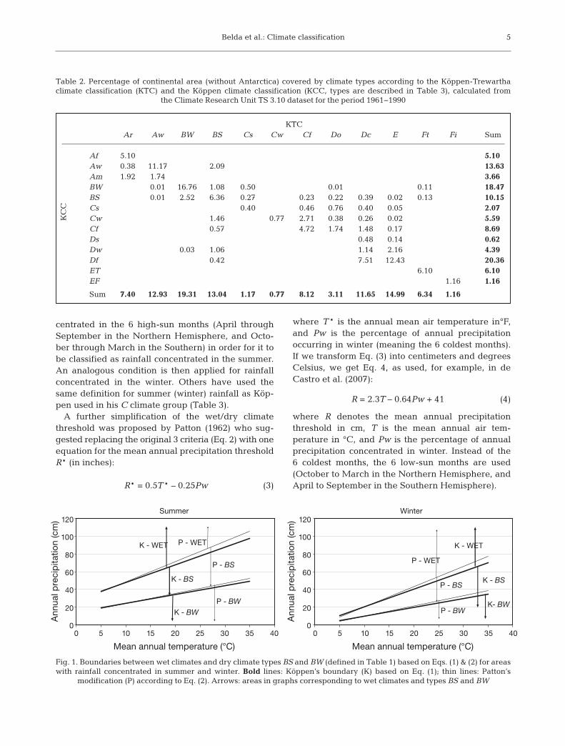
where the mean annual precipitation threshold R* isin inches, and the mean annual air temperature T* isin degrees Fahrenheit. The differences resulting fromPatton’s modification are illustrated in Fig. 1. It isobvious that the boundary between wet and dry climates is similar in areas with lower mean air temperature.

In Köppen (1923, 1931, 1936), the meaning of ‘rain-fall concentrated in summer/ winter’ is not explainedexplicitly, but it is clear that there must be a markedseasonal contrast both in rainfall and in air tem -perature. Some authors have used the condition that70% of the annual precipitation amount must be con-

4

Type / subtype CriteriaRainfall/temperature regime

A Tcold > 18°C; Pmean ≥ RAr 10 to 12 mo wet; 0 to 2 mo dryAw Winter (low-sun period) dry; >2

months dryAs Summer (high-sun period) dry; rare

in type A climates

B Pmean < RBS R/2 < Pmean < RBW Pmean < R/2

C Tcold < 18 °C; 8 to 12 months withTmo > 10°C

Cs Summer dry; at least 3 times asmuch rain in winter half year as insummer half-year; Pdry< 3 cm; totalannual precipitation < 89 cm

Cw Winter dry; at least 10 times asmuch rain in summer half-year as inwinter half-year

Cf No dry season; difference betweendriest and wettest month less thanrequired for Cs and Cw; Pdry> 3 cm

D 4 to 7 months with Tmo > 10°CDo Tcold > 0°C (or >2°C in some

locations inland)a

Dc Tcold < 0°C (or <2°C)a

E 1 to 3 months with Tmo > 10°C

F Twarm < 10°CFt Twarm > 0°CFi Twarm < 0°C

aIn the present study the boundary between subtypes Doand Dc is Tcold = 0°C

Table 1. Climate types and subtypes defined by the Köppen-Trewartha climate classification (Trewartha & Horn 1980). T:mean annual temperature (°C); Tmo: mean monthly tempera-ture (°C); Pmean: mean annual rainfall (cm); Pdry: monthly rain-fall of the driest summer month; R: Patton’s precipitationthreshold, defined as R = 2.3T − 0.64 Pw + 41, where Pw isthe percentage of annual precipitation occurring in winter(Patton 1962); Tcold (Twarm): monthly mean air temperature of

the coldest (warmest) month

Belda et al.: Climate classification

centrated in the 6 high-sun months (April throughSep tember in the Northern Hemisphere, and Octo-ber through March in the Southern) in order for it tobe classified as rainfall concentrated in the summer.An analogous condition is then applied for rainfallconcentrated in the winter. Others have used thesame definition for summer (winter) rainfall as Köp-pen used in his C climate group (Table 3).

A further simplification of the wet/dry climatethresh old was proposed by Patton (1962) who sug-gested replacing the original 3 criteria (Eq. 2) with oneequation for the mean annual precipitation thresh oldR* (in inches):

R* = 0.5T* – 0.25Pw (3)

where T* is the annual mean air temperature in°F,and Pw is the percentage of annual precipitationoccurring in winter (meaning the 6 coldest months).If we transform Eq. (3) into centimeters and degreesCelsius, we get Eq. 4, as used, for example, in deCastro et al. (2007):

R = 2.3T – 0.64Pw + 41 (4)

where R denotes the mean annual precipitationthreshold in cm, T is the mean annual air tem -perature in °C, and Pw is the percentage of annualprecipitation concentrated in winter. Instead of the6 coldest months, the 6 low-sun months are used(October to March in the Northern Hemisphere, andApril to September in the Southern Hemisphere).

5

Summer

0

20

40

60

80

100

120

0 5 10 15 20 25 30 35 40 0 5 10 15 20 25 30 35 40

Ann

ual p

reci

pita

tion

(cm

)

Ann

ual p

reci

pita

tion

(cm

)

K - BS

K - WET

K - BW

P - WET

P - BS

P - BW

Winter

0

20

40

60

80

100

120

Mean annual temperature (°C) Mean annual temperature (°C)

K- BW

K - WET

K - BS

P - WET

P - BS

P - BW

Fig. 1. Boundaries between wet climates and dry climate types BS and BW (defined in Table 1) based on Eqs. (1) & (2) for areaswith rainfall concentrated in summer and winter. Bold lines: Köppen’s boundary (K) based on Eq. (1); thin lines: Patton’s

modification (P) according to Eq. (2). Arrows: areas in graphs corresponding to wet climates and types BS and BW

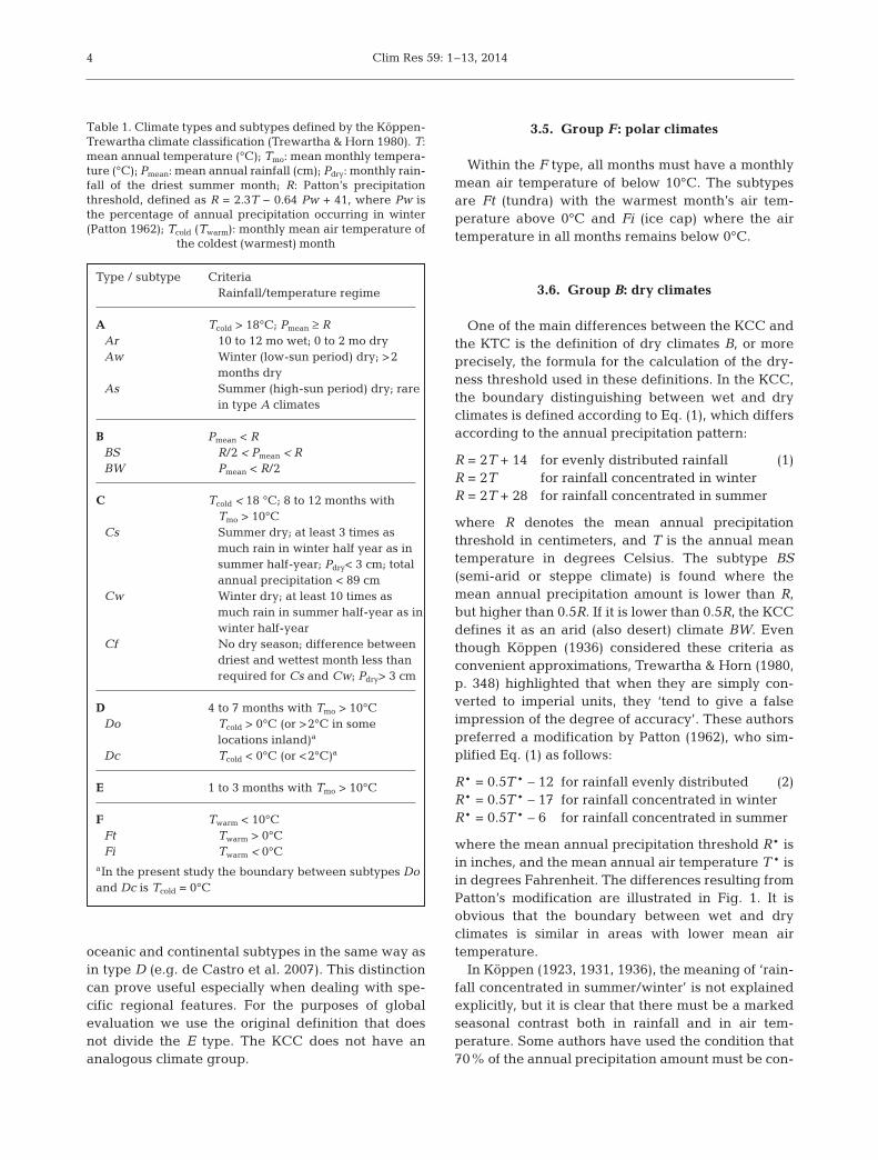
KTC Ar Aw BW BS Cs Cw Cf Do Dc E Ft Fi Sum

Af 5.10 5.10 Aw 0.38 11.17 2.09 13.63 Am 1.92 1.74 3.66 BW 0.01 16.76 1.08 0.50 0.01 0.11 18.47 BS 0.01 2.52 6.36 0.27 0.23 0.22 0.39 0.02 0.13 10.15 Cs 0.40 0.46 0.76 0.40 0.05 2.07 Cw 1.46 0.77 2.71 0.38 0.26 0.02 5.59 Cf 0.57 4.72 1.74 1.48 0.17 8.69 Ds 0.48 0.14 0.62 Dw 0.03 1.06 1.14 2.16 4.39 Df 0.42 7.51 12.43 20.36 ET 6.10 6.10 EF 1.16 1.16

Sum 7.40 12.93 19.31 13.04 1.17 0.77 8.12 3.11 11.65 14.99 6.34 1.16

Table 2. Percentage of continental area (without Antarctica) covered by climate types according to the Köppen-Trewartha climate classification (KTC) and the Köppen climate classification (KCC, types are described in Table 3), calculated from

the Climate Research Unit TS 3.10 dataset for the period 1961−1990

KC

C

Clim Res 59: 1–13, 2014

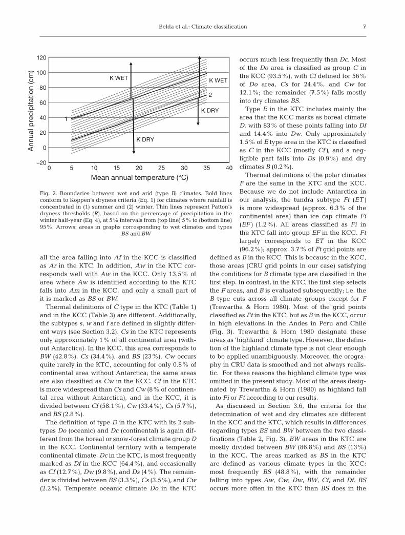
In the present study, we use Patton’s modificationas expressed by Eq. (4). The BS subtype is defined bya mean annual precipitation amount Pmean lower thanR and higher than 0.5R, and the BW subtype by amean annual precipitation lower than 0.5R. The re -sulting boundaries between wet and dry B climatetypes are illustrated in Fig. 2. Köppen’s originalboundaries (Eq. 1), in the case of rainfall concen-trated in summer and winter (bold lines 1 and 2,respectively, in Fig. 2), correspond approximately toPatton’s thresholds for Pw equal to 30 and 75%,respectively.

4. COMPARISON OF KOPPEN-TREWARTHA AND KOPPEN

CLIMATE CLASSIFICATIONS INTHE PERIOD 1961−1990

In this section, we apply both theKCC and the KTC to CRU TS3.10 anddiscuss their differences. The mapsfor both classifications are presentedin Fig. 3. The percentage of continen-tal area (except for Antarctica) clas -sified according to the KCC andthe KTC is compared in Table 2. It isimportant to acknowledge that, eventhough the designations in both classi-fications are mostly the same, the defi-nitions of the types might be differentin many respects. It is worth notingthat in the KTC as described in Tre-wartha & Horn (1980), the subtype Cwis barely mentioned, and similarly, inthe KCC (Köppen 1936), the subtypesAs and Ds are considered as rarely oc-curring. Therefore, we did not incor-porate As in our analysis. The Ds sub-type was also considered in this study;however, it was confirmed that, in theCRU data for the period 1961−1990, itis present in only a very small numberof grid points (Table 2).

From Fig. 3, the benefit of the KTCin comparison with the KCC is evi-dent. An example is the extent of dryclimate types in the interior UnitedStates. Trewartha & Horn (1980) dis-cuss that the boundary is placed some300 to 400 km west according to original Köppen’s formulas due to un -der estimation of the dryness thresh-old. KTC is much more realistic inplacing this boundary. In Europe, we

see a clear division of the western and eastern partsbetween types Dc and Do in the KTC. In other words,the KTC provides a more detailed description of cli-mate types than the KCC.

From Table 2, it can be seen that the definitionof climate type A is practically the same in boththe KCC and the KTC. The Ar subtype in the KTCis very similar to Af in the KCC; therefore, mostof the con tinental area classified as Ar correspondsto Af in the KCC (69% of continents without Ant -arctica). The remainder is divided between Am(25.9%) and Aw (5.1%) in the KCC. Interestingly,

6

Type/Subtype CriteriaRainfall/temperature regime

A Tcold > 18°C; Pmean above value given for BAf Pmo ≥ 60 mm for all monthsAw Pmo < 60 mm for several months; dry season in low-sun

period or winter half-year; annual rainfall insufficient tocompensate this enough to allow forest

As Pmo < 60 mm for several months; dry season in high-sunperiod or summer half-year; annual rainfall insufficientto compensate this enough to allow forest (occursrarely)

Am Pdry < 60 mm, rainfall in the rainy season compensatesthis enough to allow foresta

B Pmax in summer: Pmean < 2T + 28; Pmax in winter: Pmean < 2T;annual rainfall evenly distributed: Pmean < 2T + 14

BS Pmax in summer: (2T + 28)/2 < Pmean < 2T + 28 Pmax in winter: (2T)/2 < Pmean < 2TAnnual rainfall evenly distributed: (2T + 14)/2 < Pmean < 2T + 14

BW Pmax in summer: Pmean < (2T + 28)/2Pmax in winter: Pmean < (2T)/2 Annual rainfall evenly distributed: Pmean < (2T + 14)/2

C Tcold from 18 to –3°C; Twarm > 10°C; Pmean above value given in B

Cs Summer dry; wettest (winter) month must have morethan 3 times the average rainfall of the driest (summer)month; Pdry < 40 mm

Cw Winter dry; wettest (summer) month has ≥10 times therainfall of the driest (winter) month

Cf No dry season

D Tcold < –3°C; Twarm > 10°C; Pmean above value given in BDs Summer dry (the same condition as in Cs) (occurs rarely)Dw Winter dry (the same condition as in Cw)Df No dry season

E Twarm < 10°CET 0°C < Twarm < 10°CEF Mean air temperature of all months < 0°C

aKöppen (1936) describes the relationship between necessary annual rain -fall P (cm) and monthly rainfall of the driest month Pdry (cm) in the form ofgraph; it can be expressed as Pdry = −0.04P + 10

Table 3. Climate types and subtypes defined by the Köppen climate classi -fication (KCC) (Köppen 1936). Pmax: maximum annual precipitation rainfall;

Pmo: monthly precipitation; Other abbreviations as in Table 1

Belda et al.: Climate classification

all the area falling into Af in the KCC is classifiedas Ar in the KTC. In addition, Aw in the KTC cor-responds well with Aw in the KCC. Only 13.5% ofarea where Aw is identified according to the KTCfalls into Am in the KCC, and only a small part ofit is marked as BS or BW.

Thermal definitions of C type in the KTC (Table 1)and in the KCC (Table 3) are different. Additionally,the subtypes s, w and f are defined in slightly differ-ent ways (see Section 3.2). Cs in the KTC representsonly approximately 1% of all continental area (with-out Antarctica). In the KCC, this area corresponds toBW (42.8%), Cs (34.4%), and BS (23%). Cw occursquite rarely in the KTC, accounting for only 0.8% ofcontinental area without Antarctica; the same areasare also classified as Cw in the KCC. Cf in the KTCis more widespread than Cs and Cw (8% of continen-tal area without Antarctica), and in the KCC, it isdivided between Cf (58.1%), Cw (33.4%), Cs (5.7%),and BS (2.8%).

The definition of type D in the KTC with its 2 sub-types Do (oceanic) and Dc (continental) is again dif-ferent from the boreal or snow-forest climate group Din the KCC. Continental territory with a temperatecontinental climate, Dc in the KTC, is most frequentlymarked as Df in the KCC (64.4%), and occasionallyas Cf (12.7%), Dw (9.8%), and Ds (4%). The remain-der is divided between BS (3.3%), Cs (3.5%), and Cw(2.2%). Temperate oceanic climate Do in the KTC

occurs much less frequently than Dc. Mostof the Do area is classified as group C inthe KCC (93.5%), with Cf de fined for 56%of Do area, Cs for 24.4%, and Cw for12.1%; the remainder (7.5%) falls mostlyinto dry climates BS.

Type E in the KTC includes mainly thearea that the KCC marks as boreal climateD, with 83% of these points falling into Dfand 14.4% into Dw. Only approximately1.5% of E type area in the KTC is classifiedas C in the KCC (mostly Cf), and a neg -ligible part falls into Ds (0.9%) and dry climates B (0.2%).

Thermal definitions of the polar climatesF are the same in the KTC and the KCC.Because we do not include Antarctica inour analysis, the tundra subtype Ft (ET)is more widespread (approx. 6.3% of thecontinental area) than ice cap climate Fi(EF) (1.2%). All areas classified as Fi inthe KTC fall into group EF in the KCC. Ftlargely corresponds to ET in the KCC(96.2%); approx. 3.7% of Ft grid points are

defined as B in the KCC. This is because in the KCC,those areas (CRU grid points in our case) satisfyingthe conditions for B climate type are classified in thefirst step. In contrast, in the KTC, the first step selectsthe F areas, and B is evaluated subsequently; i.e. theB type cuts across all climate groups except for F(Trewartha & Horn 1980). Most of the grid pointsclassified as Ft in the KTC, but as B in the KCC, occurin high elevations in the Andes in Peru and Chile(Fig. 3). Trewartha & Horn 1980 designate theseareas as ‘highland’ climate type. However, the defini-tion of the highland climate type is not clear enoughto be applied unambiguously. Moreover, the orogra-phy in CRU data is smoothed and not always realis-tic. For these reasons the highland climate type wasomitted in the present study. Most of the areas desig-nated by Trewartha & Horn (1980) as highland fallinto Fi or Ft according to our results.

As discussed in Section 3.6, the criteria for thedetermination of wet and dry climates are differentin the KCC and the KTC, which results in differencesregarding types BS and BW between the two classi -fications (Table 2, Fig. 3). BW areas in the KTC aremostly divided between BW (86.8%) and BS (13%)in the KCC. The areas marked as BS in the KTCare defined as various climate types in the KCC:most frequently BS (48.8%), with the remainderfalling into types Aw, Cw, Dw, BW, Cf, and Df. BSoccurs more often in the KTC than BS does in the

7

–20

0

20

40

60

80

100

120

0 5 10 15 20 25 30 35 40

Mean annual temperature (°C)

Ann

ual p

reci

pita

tion

(cm

)

K WET

2

K DRY

1K DRY

K WET

Fig. 2. Boundaries between wet and arid (type B) climates. Bold lines conform to Köppen’s dryness criteria (Eq. 1) for climates where rainfall isconcentrated in (1) summer and (2) winter. Thin lines represent Patton’sdryness thresholds (R), based on the percentage of precipitation in thewinter half-year (Eq. 4), at 5% intervals from (top line) 5% to (bottom line)95%. Arrows: areas in graphs corresponding to wet climates and types

BS and BW

Clim Res 59: 1–13, 20148

Fig. 3. World maps of Köppen climate classification KCC and Köppen-Trewartha climate classification KTC, based on CRU TS 3.10 data for the period of 1961−1990 on a regular 0.5° latitude/longitude grid

Belda et al.: Climate classification

KCC. The percentage of areas classified as BW isvery similar in both classifications (approx. 19% ofcontinental area).

5. KOPPEN-TREWARTHA CLIMATE TYPES OVERTHE PERIOD 1901−2005

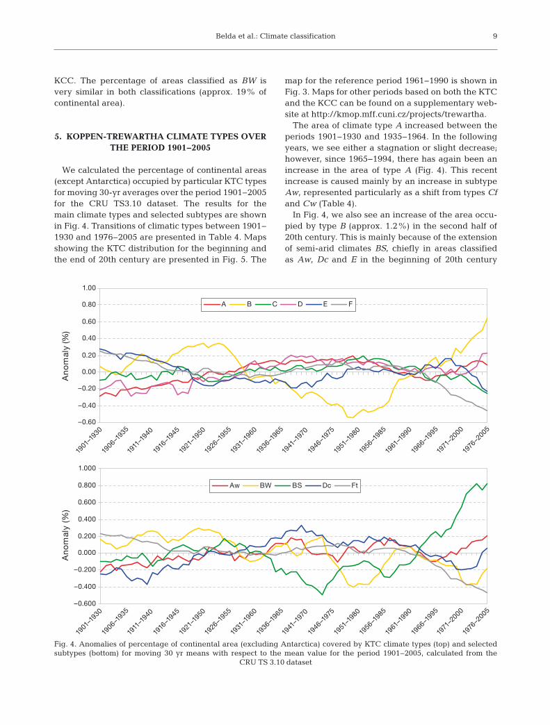
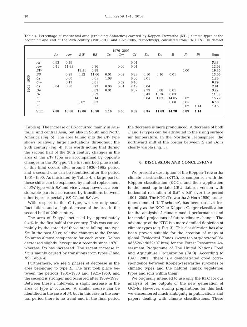
We calculated the percentage of continental areas(except Antarctica) occupied by particular KTC typesfor moving 30-yr averages over the period 1901−2005for the CRU TS3.10 dataset. The results for themain climate types and selected subtypes are shownin Fig. 4. Transitions of climatic types be tween 1901−1930 and 1976−2005 are presented in Table 4. Mapsshowing the KTC distribution for the beginning andthe end of 20th century are presented in Fig. 5. The

map for the reference period 1961−1990 is shown inFig. 3. Maps for other pe riods based on both the KTCand the KCC can be found on a supplementary web-site at http:// kmop. mff.cuni.cz/projects/trewartha.

The area of climate type A increased between theperiods 1901−1930 and 1935−1964. In the followingyears, we see either a stagnation or slight decrease;however, since 1965−1994, there has again been anincrease in the area of type A (Fig. 4). This recentincrease is caused mainly by an increase in subtypeAw, represented particularly as a shift from types Cfand Cw (Table 4).

In Fig. 4, we also see an increase of the area occu-pied by type B (approx. 1.2%) in the second half of20th century. This is mainly because of the extensionof semi-arid climates BS, chiefly in areas classifiedas Aw, Dc and E in the beginning of 20th century

9

–0.60

–0.40

–0.20

0.00

0.20

0.40

0.60

0.80

1.00

1901

–193

0

1906

–193

5

1911

–194

0

1916

–194

5

1921

–195

0

1926

–195

5

1931

–196

0

1936

–196

5

1941

–197

0

1946

–197

5

1951

–198

0

1956

–198

5

1961

–199

0

1966

–199

5

1971

–2000

1976

–2005

1901

–193

0

1906

–193

5

1911

–194

0

1916

–194

5

1921

–195

0

1926

–195

5

1931

–196

0

1936

–196

5

1941

–197

0

1946

–197

5

1951

–198

0

1956

–198

5

1961

–199

0

1966

–199

5

1971

–2000

1976

–2005

An

om

aly

(%)

A B C D E F

–0.600

–0.400

–0.200

0.000

0.200

0.400

0.600

0.800

1.000

An

om

aly

(%)

Aw BW BS Dc Ft

Fig. 4. Anomalies of percentage of continental area (excluding Antarctica) covered by KTC climate types (top) and selectedsubtypes (bottom) for moving 30 yr means with respect to the mean value for the period 1901−2005, calculated from the

CRU TS 3.10 dataset

Clim Res 59: 1–13, 2014

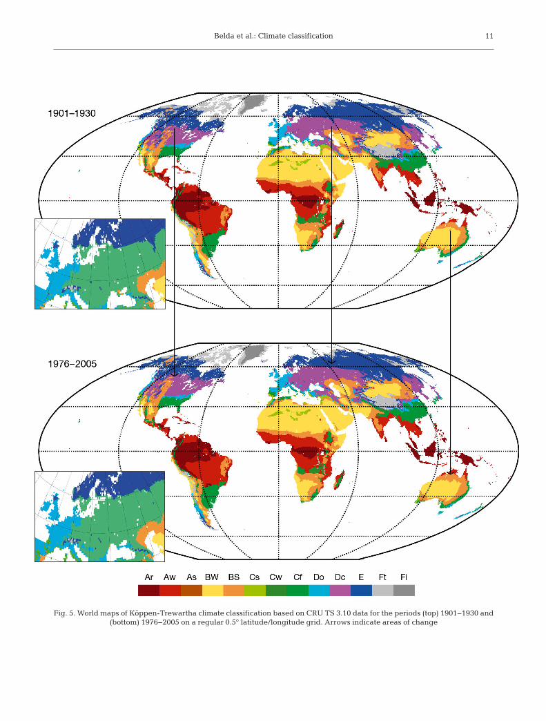
(Table 4). The increase of BS occurred mainly in Aus-tralia, and central Asia, but also in South and NorthAmerica (Fig. 5). The area falling into the BW typeshows relatively large fluctuations throughout the20th century (Fig. 4). It is worth noting that duringthe second half of the 20th century changes in thearea of the BW type are accompanied by oppositechanges in the BS type. The first marked phase shiftof this kind occurs after around 1936−1965 periodand a second one can be identified after the period1961−1990. As illustrated by Table 4, a large part ofthese shifts can be explained by mutual replacementof BW type with BS and vice versa; however, a con-siderable part is also caused by transitions betweenother types, especially BS-Cf and BS-Aw.

With respect to the C type, we see only small fluctuations and a slight decrease of the area in thesecond half of 20th century.

The area of D type increased by approximately0.4% in the first half of the century. This was causedmainly by the spread of those areas falling into typeDc. In the past 50 yr, relative changes to the Dc andDo areas almost compensate for each other; Dc hasdecreased slightly (except most recently since 1970),whereas Do has increased. The recent increase inDc is mainly caused by transitions from types E andBS (Table 4).

Furthermore, we see 2 phases of decrease in thearea belonging to type E. The first took place be -tween the periods 1901−1930 and 1921−1950, andthe second is stronger and occurred after 1969−1998.Between these 2 intervals, a slight increase in thearea of type E occurred. A similar course can be identified in the case of Ft, but in this case in the cen-tral period there is no trend and in the final period

the decrease is more pronounced. A decrease of bothE and Ft types can be attributed to the rising surfaceair temperature. In the Northern Hemisphere, thenorthward shift of the border between E and Dc isclearly visible (Fig. 5).

6. DISCUSSION AND CONCLUSIONS

We present a description of the Köppen-Trewarthaclimate classification (KTC), its comparison with theKöppen classification (KCC), and their applicationto the most up-to-date CRU dataset version with horizontal resolution of 0.5° × 0.5° over the period1901−2005. The KTC (Trewartha & Horn 1980), some -times denoted ‘K-T scheme’, has been used as fre-quently as the KCC or Köppen-Geiger classificationfor the analysis of climate model performance andfor model projections of future climate change. Theadvantage of the KTC is a more detailed depiction ofclimate types (e.g. Fig. 3). This classification has alsobeen proven suitable for the creation of maps ofglobal Ecological Zones (www.fao.org/ docrep/ 006/ad652e/ ad652e07.htm) for the Forest Resources As -sessment Programme of The United Nations Foodand Agriculture Organization (FAO). According toFAO (2001), ‘there is a demonstrated good corre-spondence between Köppen-Trewartha subzones orclimatic types and the natural climax vegetationtypes and soils within them’.

We originally intended to use only the KTC for ouranalysis of the outputs of the new generation ofGCMs. However, during preparations for this taskwe encountered much ambiguity in publications andpapers dealing with climate classifications. These

10

1976−2005 Ar Aw BW BS Cs Cw Cf Do Dc E Ft Fi Sum

Ar 6.93 0.49 0.01 7.43 Aw 0.41 11.85 0.36 0.00 0.01 12.63 BW 18.51 0.88 0.00 19.40 BS 0.29 0.52 11.66 0.01 0.02 0.29 0.10 0.16 0.01 13.06 Cs 0.00 0.05 1.08 0.05 0.01 1.20 Cw 0.13 0.05 0.52 0.10 0.79 Cf 0.04 0.30 0.27 0.06 0.01 7.19 0.04 7.91 Do 0.03 0.01 0.37 2.73 0.08 0.01 3.22 Dc 0.52 0.43 10.36 0.03 11.33 E 0.14 0.04 1.03 14.05 0.02 15.29 Ft 0.02 0.03 0.68 5.85 6.58 Fi 0.02 1.14 1.16

Sum 7.38 13.06 19.06 13.98 1.16 0.56 8.02 3.35 11.63 14.78 5.89 1.14

Table 4. Percentage of continental area (excluding Antarctica) covered by Köppen-Trewartha (KTC) climate types at the beginning and end of the 20th century (1901−1930 and 1976−2005, respectively), calculated from CRU TS 3.10 dataset

1901

–193

0

Belda et al.: Climate classification 11

Fig. 5. World maps of Köppen-Trewartha climate classification based on CRU TS 3.10 data for the periods (top) 1901−1930 and (bottom) 1976−2005 on a regular 0.5° latitude/longitude grid. Arrows indicate areas of change

Clim Res 59: 1–13, 201412

issues related to the designation of the clas sification(some studies by title suggest the KCC, but actuallyuse the KTC), modified values of thresh olds, and dif-ferent interpretations of classification algorithms, e.g.whether to apply the dryness criteria first or to setapart polar climates. Therefore, we decided to firstanalyze and describe the KTC in detail, according toTrewartha & Horn (1980) using Patton’s criteria ofdryness, and compare it to the widely used KCCscheme (Köppen 1936). Following this preparatorystudy, the analysis of the validation and of future sim-ulated climate change by using the CMIP5 GCM out-puts, will follow in subsequent papers.

Another motivation for our study is that the digitalmaps of Köppen-Geiger climate types are alreadyavailable in various versions (Kottek et al. 2006, Peelet al. 2007, Rubel & Kottek 2010). However, to ourknowledge, digital maps of the KTC climate types forthe up-to-date CRU data have not been presentedbefore. We believe that making these maps acces -sible via the internet will be beneficial to otherresearchers, not just in the field of climatology, butalso in the fields of hydrology and ecology, etc.

It is hardly possible to directly compare our resultsregarding the spatial distribution of the KTC typesand areas belonging to particular climate types withother studies because of the differences in the analyzed datasets and time periods. For example,according to the present study, the order of climatetypes ranked by the percentage of continents (ex -cluding Antarctica) that they cover in the period1976−2005 is as follows: B (33.04%), A (20.44%),D (14.98%), E (14.78%), C (9.74%), and F (7.03%).Fraedrich et al. (2001) show that for the period1981−1995 global tropical zone A covers around22.4% of the continental area. Rubel & Kottek (2010)rank type B according to KCC as the most abundant,covering total 29.14% of the global land area (includ-ing Antarctica). The ranking derived in this studyfrom the CRU data is different from the one men-tioned by Trewartha & Horn (1980), who present typeA as ‘the most widespread of any great climaticgroups’, estimating the area covered by the type A tobe around 20% of the land surface.

Regarding the changes in the area covered by indi-vidual climate types observed during 1901−2005, wehave shown that there are observable changes, espe-cially in subtypes BS, Aw and Ft (Fig. 4). Comparisonof our results concerning the temporal evolution ofthe cover of climate types with other studies is againsomewhat difficult. Temporal variations of tundra Ftagree well with the findings of Feng et al. (2012),who found a weak trend towards reduced tundra

cover from the beginning of the 20th century to the1940s and a more abrupt decrease during the past40 yr. This is also in accordance with trends de -scribed by Wang & Overland (2004) and Fraedrich etal. (2001). Furthermore, Feng et al. (2012) describean expansion of continental temperate climate Dc inthe area north of 50° N over the past few decades.In our global analysis, the Dc area has expanded inthe 30-yr periods since 1970 (Fig. 4). Fraedrich et al.(2001) found that the global tropics (A) and the tun-dra (Ft) types show statistically significant shifts inthe 1901−1995 period. The expansion of the A typewas replaced by an areal reduction near the end ofthe period. Similar to our results concerning the Ftsubtype, they also found a negative trend both at thebeginning and at the end of the 20th century.

The analysis of the time development of climatetypes was, however, not the main goal of the presentstudy; we intended primarily to prepare the back-ground for the validation and the analysis of theCMIP5 GCMs outputs in subsequent papers, wherethe temporal evolution will be addressed both forsimulations of the 20th century and future projections.Therefore, a more detailed examination of this issueis beyond the scope of this study. Here we were onlyable to show a part of the results obtained during ouranalysis. Additional materials, including digital mapsfor various time periods and animations, are accessi-ble at http:// kmop.mff.cuni. cz/ projects/trewartha.

Acknowledgements. The CRU TS 3.10.01 dataset was pro-vided by the Climatic Research Unit, University of East An-glia. This study was supported by project UNCE 204020/ 2012funded by the Charles University in Prague and by researchplan no. MSM0021620860 funded by the Ministry of Educa-tion, Youth and Sports of the Czech Republic. In addition, thework is a part of the activity under the Program of CharlesUniversity PRVOUK No. 02 ‘Environmental Research’.

LITERATURE CITED

Bailey RG (2009) Ecosystem geography: from ecoregions tosites, 2nd edn. Springer, New York, NY

Baker B, Diaz H, Hargrove W, Hoffman F (2010) Use of theKöppen-Trewartha climate classification to evaluate cli-matic refugia in statistically derived ecoregions for thePeople’s Republic of China. Clim Change 98: 113−131

Daly C, Gibson WP, Taylor GH, Johnson GL, Pasteris P(2002) A knowledge-based approach to the statisticalmapping of climate. Clim Res 22: 99−113

de Castro M, Gallardo C, Jylha K, Tuomenvirta H (2007) Theuse of a climate-type classification for assessing climatechange effects in Europe form an ensemble of nineregional climate models. Clim Change 81: 329−341

Feng S, Ho CH, Hu Q, Oglesby RJ, Jeong SJ, Kim BM (2012)

Belda et al.: Climate classification

Evaluating observed and projected future climate changesfor the Artic using the Köppen-Trewartha climate classi-fication. Clim Dyn 38: 1359−1373

Food and Agricultural Organization (FAO) (2001) Globaleco logical zoning for the Global Forest Resources Assess -ment 2000. Final Report, Forest Resources Assessment,Working Paper No. 56. FAO, Rome

Fraedrich K, Gerstengarbe FW, Werner PC (2001) Climateshifts during the last century. Clim Change 50: 405−417

Geiger R (1954) Klassifikationen der Klimate nach W. Köp-pen. In: Landolf-Börnstein: Zahlenwerte und Funktionenaus Physik, Chemie, Astronomie, Geophysik und Tech-nik, (alte Serie), Vol. 3. Springer, Berlin, p 603−607

Geiger R (1961) berarbeitete Neuausgabe von Geiger, R: Köppen-Geiger/Klima der Erde. Wandkarte (wall map)1: 16 Mill. Klett-Perthes, Gotha

Gerstengarbe FW, Werner PC (2009) A short update onKoeppen climate shifts in Europe between 1901 and2003. Clim Change 92: 99−107

Guetter PJ, Kutzbach JE (1990) A modified Koeppen classification applied to model simulation of glacial andinterglacial climates. Clim Change 16: 193−215

Harris I, Jones PD, Osborn TJ, Lister DH (in press) Updatedhigh-resolution grids of monthly climatic observations −the CRU TS3.10 dataset. Int J Clim, doi: 10.1002/joc.3711

Jones PD, Wigley TML, Farmer G (1991) Marine and landtemperature data sets: a comparison and a look at recenttrends. In: Schlesinger ME (ed) Greenhouse-gas-inducedclimatic change: a critical appraisal of simulations andobservations. Elsevier, Amsterdam, p 153−172

Kalnay E, Kanamitsu M, Kistler R, Collins W and others(1996) The NCEP/NCAR 40-year reanalysis project. BullAm Meteorol Soc 77: 437−471

Kalvová J, Halenka T, Bezpalcová K, Nemešová I (2003)Köppen climate types in observed and simulated cli-mates. Stud Geophys Geod 47: 185−202

Köppen W (1923) Die Klimate der Erde. Grundriss der Klimakunde. Walter de Gruyter, Berlin

Köppen W (1931) Grundriss der Klimakunde. Walter deGruyter, Berlin

Köppen W (1936) Das geographische System der Klimate.In: Köppen W, Geiger R (eds) Handbuch der Klimato -logie. Gebrüder Borntraeger, Berlin, p 1−44

Kottek M, Grieser J, Beck C, Rudolf B, Rubel F (2006) Worldmap of the Köppen-Geiger climate classification up -dated. Meteorol Z 15: 259−263

Legates DR, Willmott CJ (1990) Mean seasonal and spatialvariability in gauge-corrected, global precipitation. Int JClimatol 10: 111−127

Lohmann U, Sausen R, Bengtsson L, Cubash U, Perlwitz J,Roeckner E (1993) The Köppen climate classification as a

diagnostic tool for general circulation models. Clim Res3: 177−193

Meehl GA, Covey C, Delwort T, Latif M and others (2007)The WCRP CMIP3 multi-model dataset: a new era in climate change research. Bull Am Meteorol Soc 88: 1383−1394

Mitchell TD, Jones PD (2005) An improved method of con-structing a database of monthly climate observationsand associated high-resolution grids. Int J Climatol 25: 693−712

Mitchell TD, Carter TR, Jones PD, Hulme M, New M (2004)A comprehensive set of high-resolution grids of monthlyclimate for Europe and the globe: the observed records(1901−2000) and 16 scenarios (2001−2100). WorkingPaper 55, Tyndall Centre of Climate Change Research,Norwich

Nakicenovic N, Swart R (eds) (2000) Emission scenarios.Cambridge University Press, Cambridge

New M, Hulme M (1998) Development of an observedmonthly surface climate dataset over global land areasfor 1901−1995. Report, Climatic Research Unit, Univer-sity of East Anglia, Norwich

New M, Hulme M, Jones P (1999) Representing twentieth-century space-time climate variability. I. Developmentof a 1961−1990 mean monthly terrestrial climato logy.J Clim 12: 829−856

New M, Hulme M, Jones P (2000) Representing twentieth-century space–time climate variability. II. Developmentof 1901−96 monthly grids of terrestrial surface tempera-ture. J Clim 13: 2217−2238

Patton CP (1962) A note on the classification of dry climatein the Köppen system. California Geographer 3: 105−112

Peel MC, Finlayson BL, McMahon TA (2007) Updated worldmap of the Köppen-Geiger climate classification. HydrolEarth Syst Sci 11: 1633−1644

Peterson TC, Vose RS (1997) An overview of the Global His-torical Climatology Network temperature database. BullAm Meteorol Soc 78: 2837−2849

Rubel F, Kottek M (2010) Observed and projected climateshifts 1901−2100 depicted by world maps of the Köppen-Geiger climate classification. Meteorol Z 19: 135−141

Taylor K, Stouffer RJ, Meehl GA (2012) An overview ofCMIP5 and the experiment design. Bull Am MeteorolSoc 93: 485−498

Trewartha GT (1968) An introduction to climate. McGraw-Hill, New York, NY

Trewartha GT, Horn LH (1980) Introduction to climate, 5thedn. McGraw Hill, New York, NY

Wang M, Overland JE (2004) Detecting arctic climatechange using Köppen climate classification. Clim Change67: 43−62

13

Editorial responsibility: Tim Sparks, Cambridge, UK

Submitted: June 17, 2013; Accepted: October 21, 2013Proofs received from author(s): January 17, 2014