classification - logistic regression, cart (rpart) and ... · logistic regression cart regression...
TRANSCRIPT

ClassificationLogistic regression, CART (rpart) and Random Forest
COWIDUR
Torben [email protected]
Department of Mathematical Sciences
37
Classification
1 Classification
Logistic regression
CART
Regression
Classification
Example
Estimation
Partitioning
Model complexity
Pruning
Surrogates
Random Forests
Torben [email protected]
Terminology
I Supervised learning (“labelled” training data)
I ClassificationI Regression
I Unsupervised learning (describe hidden structure from“unlabelled” data)
I PCAI Clustering (K -means, . . . )
37
Classification
2 Classification
Logistic regression
CART
Regression
Classification
Example
Estimation
Partitioning
Model complexity
Pruning
Surrogates
Random Forests
Torben [email protected]
Supervised learning
I Regression
I Explain/predict a number Y fromcovariates/predictors/features/explanatory variables
I Classification
I Now Y is not a number, but a qualitative variableI Y = Eye color ∈ {green, blue, brown}I Y = E-mail type ∈ {Spam,Not spam}
I Supervised: Training data is label-ed (we know Y !!)
37
Classification
3 Classification
Logistic regression
CART
Regression
Classification
Example
Estimation
Partitioning
Model complexity
Pruning
Surrogates
Random Forests
Torben [email protected]
Classification
I Given a feature vector x and a qualitative response Ytaking values in the set C , the classification task is tobuild a function f (x) that takes as input the featurevector x and predicts its value for Y ; i.e. f (x) ∈ C
I Often: interested in estimating the probabilities that Xbelongs to each category in C
There are many methods for classification.
I Logistic regression
I Classification (and regression) trees
I Support Vector Machines
I (Artificial) Neural Networks
I k-Nearest Neighbours
I Discriminant analysis
I Naıve Bayes
I . . .
37
Classification
4 Classification
Logistic regression
CART
Regression
Classification
Example
Estimation
Partitioning
Model complexity
Pruning
Surrogates
Random Forests
Torben [email protected]
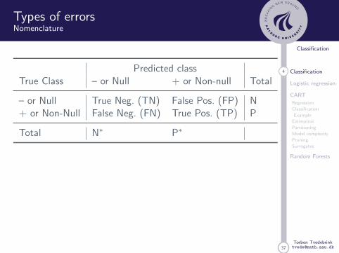
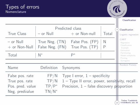
Types of errorsNomenclature
Predicted classTrue Class – or Null + or Non-null Total
– or Null True Neg. (TN) False Pos. (FP) N+ or Non-Null False Neg. (FN) True Pos. (TP) P
Total N∗ P∗
Name Definition Synonyms
False pos. rate FP/N Type I error, 1 – specificityTrue pos. rate TP/N 1 – Type II error, power, sensitivity, recallPos. pred. value TP/P∗ Precision, 1 – false discovery proportionNeg. predvalue TN/N∗
37
Classification
4 Classification
Logistic regression
CART
Regression
Classification
Example
Estimation
Partitioning
Model complexity
Pruning
Surrogates
Random Forests
Torben [email protected]
Types of errorsNomenclature
Predicted classTrue Class – or Null + or Non-null Total
– or Null True Neg. (TN) False Pos. (FP) N+ or Non-Null False Neg. (FN) True Pos. (TP) P
Total N∗ P∗
Name Definition Synonyms
False pos. rate FP/N Type I error, 1 – specificityTrue pos. rate TP/N 1 – Type II error, power, sensitivity, recallPos. pred. value TP/P∗ Precision, 1 – false discovery proportionNeg. predvalue TN/N∗
37
Classification
5 Classification
Logistic regression
CART
Regression
Classification
Example
Estimation
Partitioning
Model complexity
Pruning
Surrogates
Random Forests
Torben [email protected]
ROC curvesDetermining alternative threshold
The Receiver Operating Characteristic (ROC) curve is usedto assess the accuracy of a continuous measurement forpredicting a binary outcome.
The accuracy of a diagnostic test can be evaluated byconsidering the two possible types of errors: false positives,and false negatives.
For a continuous measurement that we denote as M,convention dictates that a test positive is defined as Mexceeding some fixed threshold c : M > c.
In reference to the binary outcome that we denote as D, agood outcome of the test is when the test is positive amongan individual who truly has a disease: D = 1. A bad outcomeis when the test is positive among an individual who doesnot have the disease D = 0
37
Classification
5 Classification
Logistic regression
CART
Regression
Classification
Example
Estimation
Partitioning
Model complexity
Pruning
Surrogates
Random Forests
Torben [email protected]
ROC curvesDetermining alternative threshold
Formally, for a fixed cutoff c , the true positive fraction is theprobability of a test positive among the diseased population:
TPF (c) = P(M > c | D = 1)
and the false positive fraction is the probability of a testpositive among the healthy population:
FPF (c) = P(M > c | D = 0)
Since the cutoff c is not usually fixed in advance, we canplot the TPF against the FPF for all possible values of c .
This is exactly what the ROC curve is, FPF (c) on the x axisand TPF (c) along the y axis.

37
Classification
6 Classification
Logistic regression
CART
Regression
Classification
Example
Estimation
Partitioning
Model complexity
Pruning
Surrogates
Random Forests
Torben [email protected]
ROC curvesConfidence regions
It is common to compute confidence regions for points onthe ROC curve using the Clopper and Pearson (1934) exactmethod. Briefly, exact confidence intervals are calculated forthe FPF and TPF separately, each at level 1−
√1− α.
Based on result 2.4 from Pepe (2003), the cross-product ofthese intervals yields a 100%(1− α) rectangular confidenceregion for the pair.
NB! The ROC curve is only defined for two-class problemsbut has been ex- tended to handle three or more classes.Hand and Till (2001), Lachiche and Flach (2003), and Liand Fine (2008) use different approaches extending thedefinition of the ROC curve with more than two classes.

37
Classification
7 Classification
Logistic regression
CART
Regression
Classification
Example
Estimation
Partitioning
Model complexity
Pruning
Surrogates
Random Forests
Torben [email protected]
ROC curves in R
There are many packages for computing, plotting andmanuıpulating with ROC curves and other methods forclassifier visualisations.
A nice recent review by Joe Ricket (RStudio):https://rviews.rstudio.com/2019/03/01/some-r-packages-for-roc-curves/
Focus on the ROCR package:https://rocr.bioinf.mpi-sb.mpg.de/

37
Classification
8 Classification
Logistic regression
CART
Regression
Classification
Example
Estimation
Partitioning
Model complexity
Pruning
Surrogates
Random Forests
Torben [email protected]
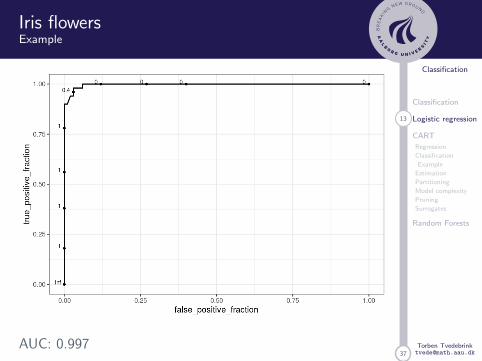
AUCArea under the curve
The overall performance of a classifier, summarised over allpossible thresholds, is given by the area under the (ROC)curve (AUC). An ideal ROC curve will hug the top leftcorner, so the larger the AUC the better the classifier.
To visually compare different models, their ROC curves canbe superimposed on the same graph. Comparing ROC curvescan be useful in contrasting two or more models withdifferent predictor sets (for the same model), different tuningparameters (i.e., within model comparisons), or completedifferent classifiers (i.e., between models).
There is a considerable amount of research on methods toformally compare multiple ROC curves. See Hanley andMcNeil (1982), DeLong et al. (1988), Venkatraman (2000),and Pepe et al. (2009) for more information.

37
Classification
Classification
9 Logistic regression
CART
Regression
Classification
Example
Estimation
Partitioning
Model complexity
Pruning
Surrogates
Random Forests
Torben [email protected]
Logistic regression
37
Classification
Classification
10 Logistic regression
CART
Regression
Classification
Example
Estimation
Partitioning
Model complexity
Pruning
Surrogates
Random Forests
Torben [email protected]
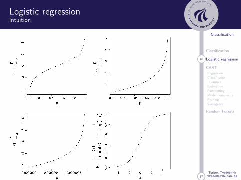
Logistic regressionIntuition
Linear regression (ignoring error term):
y = β0 + β1x
Here, y ∈ (−∞,∞), unless β1 = 0.
logit(p) = log
(p
1− p
),
logit(p) ∈ (−∞,∞) for p ∈ (0, 1).
Go from (−∞,∞) to (0, 1) (and back).
logit(p) = x ⇔ p =exp(x)
1 + exp(x)=
1
1 + exp(−x)
37
Classification
Classification
10 Logistic regression
CART
Regression
Classification
Example
Estimation
Partitioning
Model complexity
Pruning
Surrogates
Random Forests
Torben [email protected]
Logistic regressionIntuition
37
Classification
Classification
11 Logistic regression
CART
Regression
Classification
Example
Estimation
Partitioning
Model complexity
Pruning
Surrogates
Random Forests
Torben [email protected]
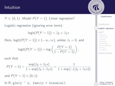
Intuition
Y ∈ {0, 1}. Model P(Y = 1). Linear regression?
Logistic regression (ignoring error term):
logit(P(Y = 1)) = β0 + β1x
Here, logit(P(Y = 1)) ∈ (−∞,∞), unless β1 = 0, and
logit(P(Y = 1)) = log
(P(Y = 1)
1− P(Y = 1)
),
such that
P(Y = 1) =exp(β0 + β1x)
1 + exp(β0 + β1x)=
1
1 + exp (−(β0 + β1x))
and P(Y = 1) ∈ (0, 1).
In R: glm(y ~ x, family = binomial).

37
Classification
Classification
12 Logistic regression
CART
Regression
Classification
Example
Estimation
Partitioning
Model complexity
Pruning
Surrogates
Random Forests
Torben [email protected]
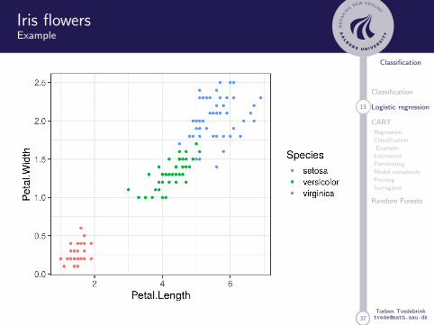
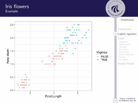
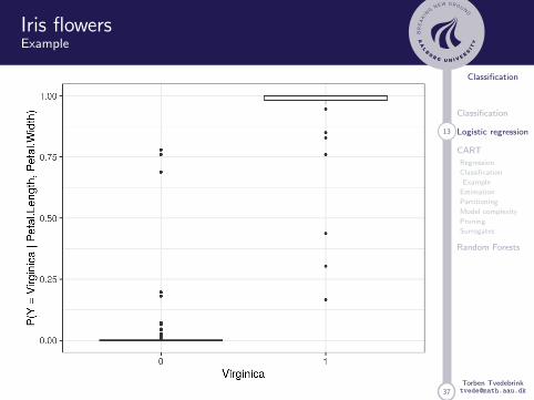
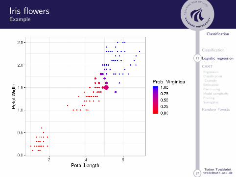
Iris Flowers
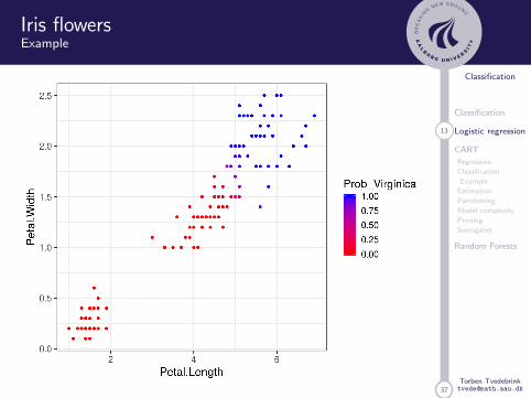
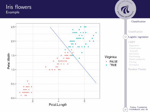
This famous (Fisher’s or Anderson’s) iris data set gives themeasurements in centimetres of the variables sepal lengthand width and petal length and width, respectively, for 50flowers from each of 3 species of iris. The species are Irissetosa, versicolor, and virginica.
Logistic regression only works for binary outcome (extensionsexist: multinomial regression, nnet::multinom)
37
Classification
Classification
13 Logistic regression
CART
Regression
Classification
Example
Estimation
Partitioning
Model complexity
Pruning
Surrogates
Random Forests
Torben [email protected]
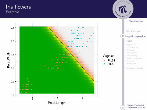
Iris flowersExample
37
Classification
Classification
13 Logistic regression
CART
Regression
Classification
Example
Estimation
Partitioning
Model complexity
Pruning
Surrogates
Random Forests
Torben [email protected]
Iris flowersExample
37
Classification
Classification
13 Logistic regression
CART
Regression
Classification
Example
Estimation
Partitioning
Model complexity
Pruning
Surrogates
Random Forests
Torben [email protected]
Iris flowersExample
37
Classification
Classification
13 Logistic regression
CART
Regression
Classification
Example
Estimation
Partitioning
Model complexity
Pruning
Surrogates
Random Forests
Torben [email protected]
Iris flowersExample
37
Classification
Classification
13 Logistic regression
CART
Regression
Classification
Example
Estimation
Partitioning
Model complexity
Pruning
Surrogates
Random Forests
Torben [email protected]
Iris flowersExample
37
Classification
Classification
13 Logistic regression
CART
Regression
Classification
Example
Estimation
Partitioning
Model complexity
Pruning
Surrogates
Random Forests
Torben [email protected]
Iris flowersExample
37
Classification
Classification
13 Logistic regression
CART
Regression
Classification
Example
Estimation
Partitioning
Model complexity
Pruning
Surrogates
Random Forests
Torben [email protected]
Iris flowersExample
37
Classification
Classification
13 Logistic regression
CART
Regression
Classification
Example
Estimation
Partitioning
Model complexity
Pruning
Surrogates
Random Forests
Torben [email protected]
Iris flowersExample
AUC: 0.997

37
Classification
Classification
Logistic regression
14 CART
Regression
Classification
Example
Estimation
Partitioning
Model complexity
Pruning
Surrogates
Random Forests
Torben [email protected]
Classification and Regression Trees
37
Classification
Classification
Logistic regression
15 CART
Regression
Classification
Example
Estimation
Partitioning
Model complexity
Pruning
Surrogates
Random Forests
Torben [email protected]
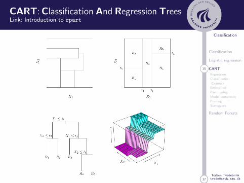
CART: Classification And Regression TreesLink: Introduction to rpart
37
Classification
Classification
Logistic regression
CART
16 Regression
Classification
Example
Estimation
Partitioning
Model complexity
Pruning
Surrogates
Random Forests
Torben [email protected]
CART: Regression
For regression the CART methodology fits a piece-wiseconstant prediction for each region Rj ,
YCART(x) =R∑j=1
βjI(x ∈ Rj),
where βj is the constant level for region Rj .
Hence, the expression for Y can be determined if
a) the partition (i.e. the regions R1, . . . ,RR) are known
b) the estimated parameters βj are known
These are chosen such that they minimises the expectedsquared loss for future observations (x , y),
E[(Y − Y )2]
37
Classification
Classification
Logistic regression
CART
Regression
17 Classification
Example
Estimation
Partitioning
Model complexity
Pruning
Surrogates
Random Forests
Torben [email protected]
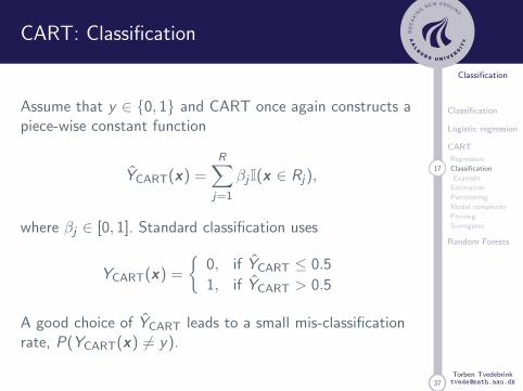
CART: Classification
Assume that y ∈ {0, 1} and CART once again constructs apiece-wise constant function
YCART(x) =R∑j=1
βjI(x ∈ Rj),
where βj ∈ [0, 1]. Standard classification uses
YCART(x) =
{0, if YCART ≤ 0.5
1, if YCART > 0.5
A good choice of YCART leads to a small mis-classificationrate, P(YCART(x) 6= y).

37
Classification
Classification
Logistic regression
CART
Regression
Classification
18 Example
Estimation
Partitioning
Model complexity
Pruning
Surrogates
Random Forests
Torben [email protected]
ExampleIris data – three species
> iris[c(1:2,51:52,101:102),]
Sepal.Length Sepal.Width Petal.Length Petal.Width Species
1 5.1 3.5 1.4 0.2 setosa
2 4.9 3.0 1.4 0.2 setosa
51 7.0 3.2 4.7 1.4 versicolor
52 6.4 3.2 4.5 1.5 versicolor
101 6.3 3.3 6.0 2.5 virginica
102 5.8 2.7 5.1 1.9 virginica
37
Classification
Classification
Logistic regression
CART
Regression
Classification
19 Example
Estimation
Partitioning
Model complexity
Pruning
Surrogates
Random Forests
Torben [email protected]
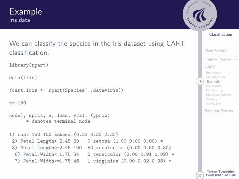
ExampleIris data
We can classify the species in the Iris dataset using CARTclassification.
library(rpart)
data(iris)
(cart.iris <- rpart(Species~.,data=iris))
n= 150
node), split, n, loss, yval, (yprob)
* denotes terminal node
1) root 150 100 setosa (0.33 0.33 0.33)
2) Petal.Length< 2.45 50 0 setosa (1.00 0.00 0.00) *
3) Petal.Length>=2.45 100 50 versicolor (0.00 0.50 0.50)
6) Petal.Width< 1.75 54 5 versicolor (0.00 0.91 0.09) *
7) Petal.Width>=1.75 46 1 virginica (0.00 0.02 0.98) *
37
Classification
Classification
Logistic regression
CART
Regression
Classification
20 Example
Estimation
Partitioning
Model complexity
Pruning
Surrogates
Random Forests
Torben [email protected]
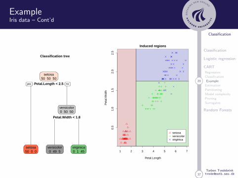
ExampleIris data – Cont’d
Classification tree
Petal.Length < 2.5
Petal.Width < 1.8
setosa50 50 50
setosa50 0 0
versicolor0 50 50
versicolor0 49 5
virginica0 1 45
yes no
1 2 3 4 5 6 7
0.5
1.0
1.5
2.0
2.5
Induced regions
Petal.Length
Pet
al.W
idth
setosaversicolorvirginica

37
Classification
Classification
Logistic regression
CART
Regression
Classification
Example
21 Estimation
Partitioning
Model complexity
Pruning
Surrogates
Random Forests
Torben [email protected]
Parameter estimation
From the model
YCART(x) =R∑j=1
βjI(x ∈ Rj),
we have that when the partitions/regions Rj are given, theMLE for βj is given by
βj =
∑ni=1 yi I(xi ∈ Rj)∑ni=1 I(xi ∈ Rj)
= yRj.
where βj for regression just is the average of the ys withx ∈ Rj and for classification the fraction of “y = 1”-samples.
37
Classification
Classification
Logistic regression
CART
Regression
Classification
Example
Estimation
22 Partitioning
Model complexity
Pruning
Surrogates
Random Forests
Torben [email protected]
Partitioning
Ideally we wants a partitioning which given the smallestexpected loss (regression: sum of squares, classification: errorrate).
The number of partitions is to vast, why an exhaustivesearch is infeasible.
Hence, we use a greedy algorithm to search for partitionswith good splits.
Note! The r in rpart stands for recursive. Hence, whatapplies to the root is used recursively down the tree.

37
Classification
Classification
Logistic regression
CART
Regression
Classification
Example
Estimation
23 Partitioning
Model complexity
Pruning
Surrogates
Random Forests
Torben [email protected]
Method to generate splits
In the training data we have {(x1, y1), . . . , (xn, yn)}, wherexi = (xi1, . . . , xip) is p-dimensional.
For a numeric predictor vector x we search for the partition:
1. Start by R1 = Rp
2. Given R1, . . . ,Rr , split each Rj into Rj1 and Rj2 where
Rj1 = {x ∈ Rp : x ∈ Rj and xk ≤ c}Rj2 = {x ∈ Rp : x ∈ Rj and xk > c},
and the variable xk with splitting points c is chosen such
arg mink,c
minβ1,β2
∑i :xi∈Rj1
(yi − β1)2 +∑
i :xi∈Rj2
(yi − β2)2
Let R11 ,R12 , . . . ,Rr1 ,Rr2 be new partitions.
3. Repeat step 2. d times to get a tree of depth d .

37
Classification
Classification
Logistic regression
CART
Regression
Classification
Example
Estimation
Partitioning
24 Model complexity
Pruning
Surrogates
Random Forests
Torben [email protected]
Model complexity
What size of tree is optimal?
We can grow the tree until each observations has its ownleaf (terminal node). This gives an error rate of null, but notvery enlightening!.
Hence, stop before that, but when?
37
Classification
Classification
Logistic regression
CART
Regression
Classification
Example
Estimation
Partitioning
25 Model complexity
Pruning
Surrogates
Random Forests
Torben [email protected]
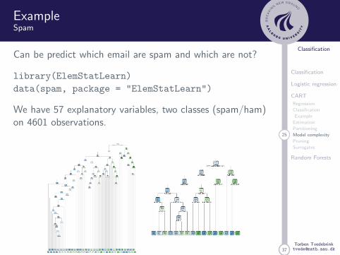
ExampleSpam
Can be predict which email are spam and which are not?
library(ElemStatLearn)
data(spam, package = "ElemStatLearn")
We have 57 explanatory variables, two classes (spam/ham)on 4601 observations.
37
Classification
Classification
Logistic regression
CART
Regression
Classification
Example
Estimation
Partitioning
26 Model complexity
Pruning
Surrogates
Random Forests
Torben [email protected]
Bias vs. variance
Which of the two previous trees for the spam data wasbetter? The difference is controlled by a tuning parameterthat decides the size of the tree (its complexity).
The larger the tree, the less bias but also a higher variancefor the test data. Conversely, smaller trees gives larger bias,but little variance for test data.
In general, a bigger tree gives a better prediction for trainingdata. However, an increased model complexity may result ina the model too specific for the training data (over-fitting!),which makes it less applicable for test data and predictionfor new data. It has a poor generalisation ability.

37
Classification
Classification
Logistic regression
CART
Regression
Classification
Example
Estimation
Partitioning
27 Model complexity
Pruning
Surrogates
Random Forests
Torben [email protected]
Choosing the optimal treeTuning parameter α
We wants to search for the optimal tree T ∗, that minimisesthe true test error, ErrorTest. This quantity is unknown, butmay be approximated using cross-validation.
The estimate/approximation is used to identify T ∗, such that
T ∗ = arg minT
ErrorTest(T )
This, however, would require an exhaustive search over allpossible trees T – which obviously is infeasible.
Using a tuning parameter α the problem can be translatedinto a one-dimensional problem.

37
Classification
Classification
Logistic regression
CART
Regression
Classification
Example
Estimation
Partitioning
Model complexity
28 Pruning
Surrogates
Random Forests
Torben [email protected]
Pruning
The tuning parameter α penalises large trees,
ErrorTrain(T ) + α|T |, (1)
where |T | is the number of leafs in the tree.
Two approaches:
I Grow the tree until (1) increases.
I Grow a full tree and prune it until (1) increases.

37
Classification
Classification
Logistic regression
CART
Regression
Classification
Example
Estimation
Partitioning
Model complexity
29 Pruning
Surrogates
Random Forests
Torben [email protected]
Selecting α
What value of α should be used? Given α ∈ R+, let Tα bethe tree that minimises
Tα = arg minT
ErrorTrain(T ) + α|T |
We wants α∗ such that the resulting tree has the minimaltest error
Tα∗ = arg minTα, α∈R+
ˆErrorTest(Tα),
where ˆErrorTest is the estimate of the test error.

37
Classification
Classification
Logistic regression
CART
Regression
Classification
Example
Estimation
Partitioning
Model complexity
30 Pruning
Surrogates
Random Forests
Torben [email protected]
Selecting αCont’d
We may plot the generalisation error ˆErrorTest for theoptimal tree using the criterion
ErrorTrain(T ) + α|T |
as a function of α.
It holds that Tα is constant in intervals I1 = [0, α1],I2 = (α1, α2], . . . , Im = (αm−1,∞]. Hence, all values α′ ∈ Ijgives the same tree, i.e. αj , Tα′ ≡ Tαj
Note, T0 og T∞ are special cases – T0 receives no penaltyfor its size (the full tree), T∞ gives the empty tree T∅.

37
Classification
Classification
Logistic regression
CART
Regression
Classification
Example
Estimation
Partitioning
Model complexity
31 Pruning
Surrogates
Random Forests
Torben [email protected]
How in rpart
To decide on α, in rpart we use printcp or plotcp.
These functions use a rewritten version of the above:
Errorα(T )
Error∞(T )=
Error(T ) + α|T |Error(T∅)
=Error(T )
Error(T∅)+
α
Error(T∅)|T |
= rel error + cp|T |,
where the error is relative to T∞ = T∅ – i.e. the ’total’variance as we don’t have any splits in T∞
The variable cp is short for ’complexity parameter’.
37
Classification
Classification
Logistic regression
CART
Regression
Classification
Example
Estimation
Partitioning
Model complexity
32 Pruning
Surrogates
Random Forests
Torben [email protected]
Choice of cp
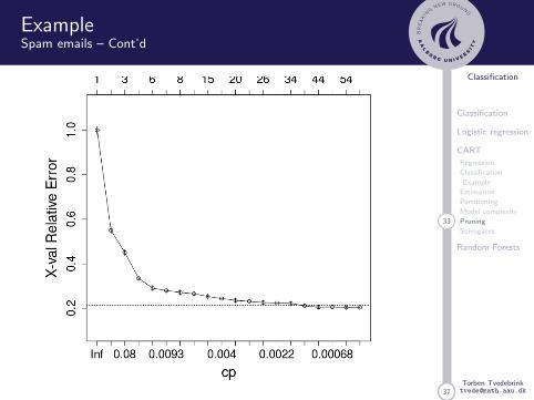
There are (at least) two criteria to select α∗ that decides thecomplexity of Tα∗ :
1. Choose cp where xerror (CV estimate of rel error)is smallest,
2. Choose cp giving xerror within one standard deviationof the smallest xerror.
In the plotcp-plot the dotted line shows xerror+xstd
relative to the cp-value with smallest xerror.
Note! xerror and xstd changes with the CV and isrecomputed for each run of rpart.
In practice we use 2. since this gives the more parsimoniousmodel (and we consider models within one standarddeviation as equally good).
37
Classification
Classification
Logistic regression
CART
Regression
Classification
Example
Estimation
Partitioning
Model complexity
33 Pruning
Surrogates
Random Forests
Torben [email protected]
ExampleSpam emails – Cont’d

37
Classification
Classification
Logistic regression
CART
Regression
Classification
Example
Estimation
Partitioning
Model complexity
34 Pruning
Surrogates
Random Forests
Torben [email protected]
ExampleSpam emails – Cont’d
library(ElemStatLearn)
data(spam, package = "ElemStatLearn")
spam_rpart <- rpart(spam ~ ., data = spam, cp = 0)
rpart.plot(spam_rpart)
plotcp(spam_rpart)
printcp(spam_rpart)
spam_rpart_prune <- prune(spam_rpart, cp = 0.004)
rpart.plot(spam_rpart_prune)
37
Classification
Classification
Logistic regression
CART
Regression
Classification
Example
Estimation
Partitioning
Model complexity
Pruning
35 Surrogates
Random Forests
Torben [email protected]
Surrogates
A nice feature of the CART methodology are the so calledsurrogates. These are variables in the data that are notchosen as primary splitting variables, but assemples thesplitting properties of the primary split.
They are in particularly important when missingobservations exists in the primary split variables.

37
Classification
Classification
Logistic regression
CART
Regression
Classification
Example
Estimation
Partitioning
Model complexity
Pruning
Surrogates
36 Random Forests
Torben [email protected]
Random Forests

37
Classification
Classification
Logistic regression
CART
Regression
Classification
Example
Estimation
Partitioning
Model complexity
Pruning
Surrogates
37 Random Forests
Torben [email protected]
Random forests
An “extension” of CART (or any tree algorithm) areRandom Forests.
Random Forests are a relatively simple, but efficientapplication of classification trees.
Random Forests use “bagging”, which is short for“bootstrap” and “aggregation”. That is, take average (ormajority decision) over many trees based on differentbootstrap samples.
37
Classification
Classification
Logistic regression
CART
Regression
Classification
Example
Estimation
Partitioning
Model complexity
Pruning
Surrogates
37 Random Forests
Torben [email protected]
Random forests
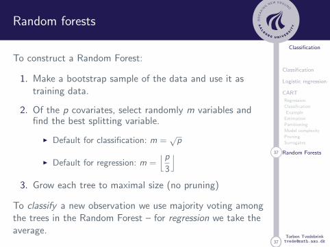
To construct a Random Forest:
1. Make a bootstrap sample of the data and use it astraining data.
2. Of the p covariates, select randomly m variables andfind the best splitting variable.
I Default for classification: m =√p
I Default for regression: m =⌊p
3
⌋3. Grow each tree to maximal size (no pruning)
To classify a new observation we use majority voting amongthe trees in the Random Forest – for regression we take theaverage.