city of rehoboth beach - dnrec draft... · city of rehoboth beach report on ocean outfall ... 1.3...
TRANSCRIPT
City of Rehoboth Beach
Report on Ocean OutfallPermitting
Assessment of thePerformance of the Rehoboth
Beach Ocean Outfall
December 2011

4 41/23409/419593Ocean Outfall PermittingAssessment of the Performance of the Rehoboth Beach Ocean Outfall
Contents
Limited Glossary of Selected Terms i
Executive Summary vii
1. Introduction 1
1.1 Project Description 1
1.2 Objectives 1
1.3 Philosophy of Modeling 1
1.4 Modeling Scope 2
1.5 Areas of Environmental Sensitivity 2
2. Literature Review 3
2.1 Garvine’s Report to Stearns and Wheler, 2003 3
2.2 Sanders, T.M., and R.W. Garvine, Fresh Water Delivery to theContinental Shelf and Subsequent Mixing: An ObservationalStudy, Journal of Geophysical Research, Vol. 106, No. C11,pages 27,087-27,101, November 15, 2001 4
2.3 Quantitative Seasonal Aspects of Zooplankton in the DelawareRiver Estuary, Chesapeake Science, Vol 3, No 2 (June 1962)pp. 63-93 5
2.4 WHITNEY, M. M., AND GARVINE, R. W., Simulating theDelaware Bay Buoyant Outflow: Comparison with Observations,Journal of Physical Oceanography, Vol 36, January 2006 6
2.5 Lawler, Matusky & Skelly Engineers, Regional Effluent DisposalStudy for the City of Rehoboth Beach, Delaware –Supplemental Dilution Modeling, 2003. 7
2.6 State of Delaware Surface Water Quality Standards, DNREC2004 8
2.7 Key Findings 9
3. Project Data 10
3.1 Short-Term Intensive Surveys 10
3.2 Long-Term Monitoring 11
3.3 Meteorological Data 14
3.4 Wave Data 20
3.5 Freshwater Inflows 21
3.6 Bathymetry 23
41/23409/419593 Ocean Outfall PermittingAssessment of the Performance of the Rehoboth Beach Ocean Outfall
4. Model Establishment and Calibration 25
4.1 Introduction 25
4.2 Governing Equations 25
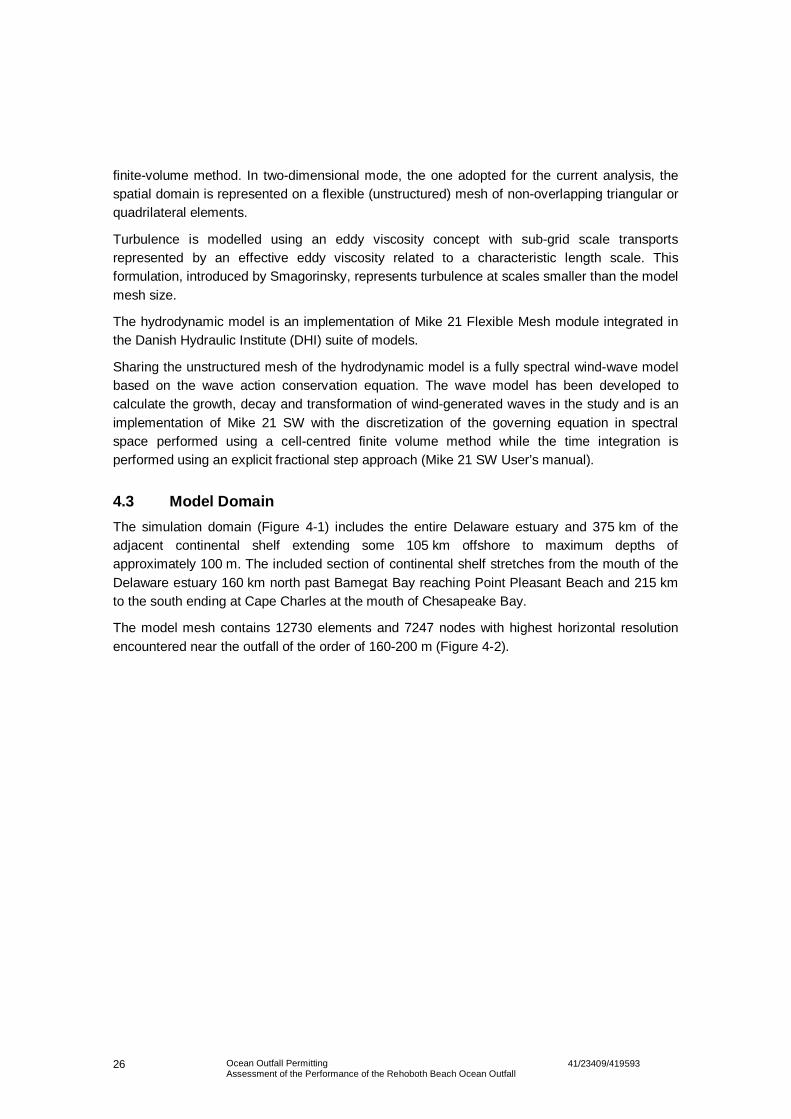
4.3 Model Domain 26
4.4 Model Operation 29
4.5 Forcing of the Hydrodynamic Model 29
4.6 Forcing of the Wave Model 29
4.7 Model Calibration 29
4.8 Model Validation 35
4.9 Verification to Previous Work 36
4.10 Conclusions 38
5. Far Field Model Results 39
5.1 Scenario Definition 39
5.2 Modeling Assumptions 39
5.3 Qualifications 40
5.4 Simulation Results 40
5.5 Conclusions 45
6. Near Field Modeling 46
6.1 Introduction 46
6.2 Aims 47
6.3 Target Dilution 47
6.4 Discharge Characteristics 48
6.5 Input Data 48
6.6 Stratification 49
6.7 Model Scenario Definition 50
6.8 Modeling Results 51
6.9 Conclusions 55
6.10 Qualifications 55
7. Conclusions and Recommendations 56
7.1 Far Field/Plume Dispersion 56
7.2 Near Field/Diffusers 56
8. References 58

6 41/23409/419593Ocean Outfall PermittingAssessment of the Performance of the Rehoboth Beach Ocean Outfall
Table IndexTable 1 Preliminary Diffuser Designs 7Table 2 Representative Current Magnitudes and Minimum
Exceedance for the Period of Measurements 14Table 3 Wind Statistics – Wind Speed/Wind Direction at
Station 44009 for the Period August 1st toDecember 31st 2010 16
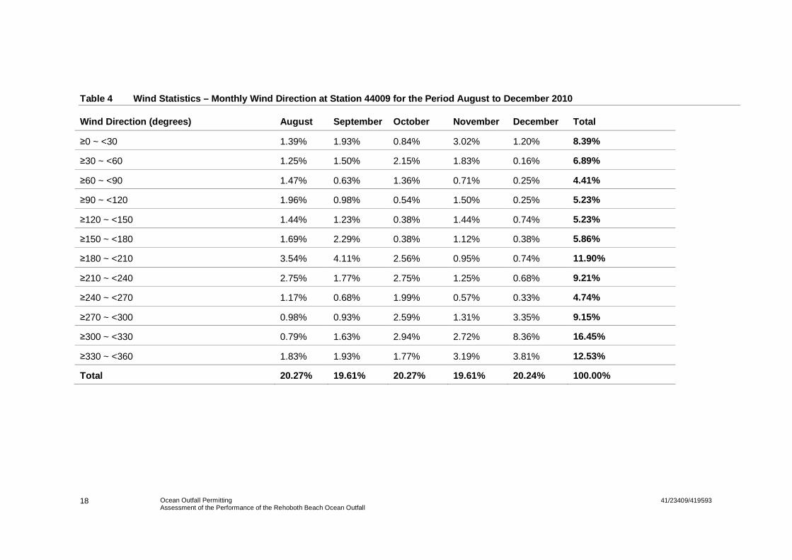
Table 4 Wind Statistics – Monthly Wind Direction at Station44009 for the Period August to December 2010 18
Table 5 Short-term Intensive Surveys - Measured DailyRiver Discharge, Associated Probability ofExceedance and Receiving Water Condition 23
Table 6 Adopted Timeframes in the Analysis (months) 40Table 7 Southern Outfall - Total Area within a Given Dilution
Contour 41Table 8 Northern Outfall - Total Area within a Given Dilution
Contour 42Table 10 Rehoboth Beach WWTP Current Effluent
Performance Data 48Table 11 Dilution Summary 53
41/23409/419593 Ocean Outfall PermittingAssessment of the Performance of the Rehoboth Beach Ocean Outfall
Figure IndexFigure 3-1 Field Data Collection Locations and Survey
Transects 11Figure 3-2 ADCP Deployment Locations 12Figure 3-3 Wind Speed/Wind Direction Percentage
Occurrence at Station 44009 for the PeriodSeptember 1st to December 31st 2010 19
Figure 3-4 Wind Speed/Wind Direction PercentageOccurrence at Station 44009 for the Period July 1st
to September 30th 2011 19Figure 3-5 Wind Speed/Wind Direction Percentage
Occurrence at Station 44009 for the Period January1st to June 30th 2011 20
Figure 3-6 Probability of Exceedance of Daily River Dischargein the Delaware River for the Period October 1st
1912 to June 12th 2011 22Figure 3-7 Comparison of Model Bathymetry versus NOAA
Charts 24Figure 4-1 Extent of the Model Used for Far-Field Analysis 27Figure 4-2 Magnified View of the Mesh of the Model at the
Proposed Outfall Site 28Figure 4-3 Comparison of ADCP records and model results:
probability of exceedance of current magnitude (toppanel), frequency histogram for current magnitude(middle panel) and frequency histogram for currentdirection (bottom panel) 34
Figure 4-4 Depth-averaged mean flow velocity for the durationof the 2010 autumn field campaign (left) and depth-averaged mean flow velocity for 1993 (right)sourced from the dissertation of Dr. M Whitney(Garvine, 2003). 36
Figure 4-5 Depth-averaged mean flow velocity (left) anddepth-averaged mean tidal velocity (right) for 1993sourced from the dissertation of Dr. M Whitney(Garvine, 2003) 37
Figure 5-1 Southern Outfall: Contour plot showing the 95th
percentile of dilution after 11 month of outfalloperation 43
Figure 5-2 Northern Outfall: Contour plot showing the 95th
percentile of dilution after 11 month of outfalloperation 44

8 41/23409/419593Ocean Outfall PermittingAssessment of the Performance of the Rehoboth Beach Ocean Outfall
Figure 6-1 Schematic Diagram of Modeled Diffuser 46Figure 6-2 Measured Current Magnitude at 8.2 ft (2.5 m)
above the seafloor (% Occurrence) 49Figure 6-3 Near-Field Dilutions for Simulation Cases 000 to
006 52Figure 6-4 Near-Field Dilutions for Simulation cases 007 and
008 52
AppendicesA Locality MapB Project DataC Model Calibration and VerificationD Far-Field ModelingE Near-Field Modeling

41/23409/419593i
Limited Glossary of Selected Terms
A
ADCP Acoustic Doppler Current Profiler – instrument used to measure currentsand wave height, period and direction. An ADCP anchored to theseafloor can measure current speed not just at the bottom, but also atequal intervals all the way up to the surface. The instrument can also bemounted to the bottoms of ships to take constant current measurementsas the boats move. In very deep areas, they can be lowered on a cablefrom the surface.
Astronomical tide The tidal levels and character which would result from gravitationaleffects, e.g. of the Earth, Sun and Moon, without any atmosphericinfluences.
B
Baroclinic flow Flow conditions in the ocean such that levels of constant pressure areinclined to surfaces of constant density. In this case, density varies withdepth and horizontal position.
Barotropic flow Flow conditions in the ocean such that levels of constant pressure arealways parallel to the surfaces of constant density.
Bathymetry The measurement of water depths in oceans, seas, and lakes; alsoinformation derived from such measurements.
C
Coriolis Force The deflection of moving objects (air and water currents) due to therotation of the Earth - to the right in the northern hemisphere, and to theleft in the southern.
Calibration Adjustment of a model’s numerical and physical parameters such asroughness or dispersion coefficients so that it reproduces observedprototype data to acceptable accuracy.
D
DHI Danish Hydraulic Institute
ii 41/23409/419593Ocean Outfall PermittingAssessment of the Performance of the Rehoboth Beach Ocean Outfall
F
Far-field The region of the receiving waters where conditions existing in theambient environment gain control over the trajectory and dilution of theturbulent plume.
Fetch The area of sea, along the direction of the wind, over which winds arerelatively constant and wave generation occurs.
Fully developed sea Sea in a quasi-steady state in which the energy gained by waves fromthe wind is approximately equal to that lost to wave breaking and othermechanisms.
G
GeographicInformation System(GIS)
A computer-based system used to capture, create, maintain, displayand analyse spatially-related information.
H
Hurricane A tropical cyclone in the Atlantic, Caribbean Sea, Gulf of Mexico, oreastern Pacific, with a maximum 1-minute sustained surface wind of 64knots (74 mph) or greater.
Hydrographic survey The measurement and description of the physical features offshore andadjoining coastal areas with special reference to their use for thepurpose of navigation.
K
Knot A nautical unit of speed defined as 1 international nautical mile per hour.The knot is equal to 1.852 km/h.
M
Magnetic Declination The observed angular distance between magnetic north on a compassand true north.
N
Nautical mile Unit of length corresponding approximately to one minute of arc oflatitude along any meridian, but is approximately one minute of arc oflongitude only at the equator. By international agreement it is exactly1,852 metres (approximately 6,076 feet).

iii41/23409/419593
Near-field The region of the receiving waters where the initial jet characteristics ordischarge conditions and the outfall geometry influence the jet trajectoryand mixing.
NOAA National Oceanic and Atmospheric Association
O
Onshore wind A wind blowing landward from the sea in the coastal area.
Offshore wind A wind blowing seaward from the land in the coastal area.
P
Primary contractrecreation
Any water-based form of recreation, the practice of which has a highprobability for total immersion or ingestion of water (examples includebut are not limited to swimming and water skiing)
R
Richardson Number The primary parameter that can be used to classify the stratificationpotential of an estuary defined as (Fischer et al., 1979)
3t
f
WUgQ
Ri where is the difference between freshwater and
seawater density, typically 25 kg/m3; is the reference density,
typically 1000 kg/m3; g is gravity (m/s2), fQ is the freshwater inflow
(m3/s); W is the width of the estuary (m); and tU is the mean tidal
velocity (m/s). If Ri is large (>0.8), the estuary is expected to bestrongly stratified and dominated by density currents, and if Ri is small(<0.08), the estuary is expected to be well mixed. Transition from a well-mixed to a strongly mixed estuary occurs in the range 8.008.0 Ri .
Regulatory mixingzone
A designated, mathematically defined portion of a receiving water body,in close proximity to a discharge, in which the initial dilution, dispersion,and reaction of discharged pollutants occur.
RMSE Root-Mean-Square-Error - a criteria for the assessment of modelperformance
iv 41/23409/419593Ocean Outfall PermittingAssessment of the Performance of the Rehoboth Beach Ocean Outfall
S
Shelf Surrounding nearly all continents is a shallow extension of thatlandmass known as the continental shelf. This shelf is relatively shallow,tens of meters deep compared to the thousands of meters deep in theopen ocean, and extends outward to the continental slope where thedeep ocean truly begins (sourced from
http://www.onr.navy.mil/focus/ocean/regions/oceanfloor2.htm)
Stratification The separation of the water column into layers.
More specifically, in the context of the Delaware Estuary, stratification isa category used for classifying a water body influenced by tides andfreshwater inflows. Three stratification classes of estuaries are:
1. Highly stratified (salt wedge) estuaries that have large riverdischarges flowing into them.
2. Partially mixed estuaries with medium river discharges.
3. Vertically homogeneous estuaries that have small river discharges.
Secondary contactrecreation
A water-based form of recreation, the practice of which has a lowprobability of for total body immersion or ingestion of water (examplesinclude but are not limited to wading, boating and fishing)
T
Tide The periodic rising and falling of the water that results from gravitationalattraction of the moon and sun and other astronomical bodies actingupon the rotating earth. Although the accompanying horizontalmovement of the water resulting from the same cause is alsosometimes called the tide, it is preferable to designate the latter asTIDAL CURRENT, reserving the name TIDE for the vertical movement.
v41/23409/419593
U
Upwelling The vertical motion of water in the ocean by which subsurface water oflower temperature and greater density moves toward the surface of theocean. Upwelling occurs most commonly among the western coastlinesof continents, but may occur anywhere in the ocean. Upwelling resultswhen winds blowing nearly parallel to a continental coastline transportthe light surface water away from the coast. Subsurface water of greaterdensity and lower temperature replaces the surface water, and exerts aconsiderable influence on the weather of coastal regions. Upwelling alsoresults in increased ocean productivity by transporting nutrient-richwaters to the surface layer of the ocean.
V
Validation Comparison of model results with a set of prototype data that were notused for calibration.

vi 41/23409/419593Ocean Outfall PermittingAssessment of the Performance of the Rehoboth Beach Ocean Outfall

vii41/23409/419593
Executive Summary
The City of Rehoboth Beach is considering building an ocean outfall for discharging effluent (wastewater)from its existing advanced secondary treatment plant. This would replace the existing point of dischargewhich occurs in the Lewes-Rehoboth Canal. At this stage two candidate locations are being consideredfor the new ocean outfall. These are referred in the text as northern and southern outfalls. Both optionsare included in the analysis to facilitate the decision-making process.
The purpose of this document is to provide support for the proposed project by (1) describing thehydrodynamics of the receiving waters offshore of Rehoboth Beach and (2) predicting the ultimate fate ofthe effluent so that potential environmental impacts can be adequately assessed.
To do so, a large-scale finite volume hydrodynamic model of the Delaware Estuary has been establishedand operated in a series of calibration scenarios involving the three most significant driving forcesgoverning the ocean hydrodynamics of the area - the tide, freshwater inflows from the Delaware Riverand offshore winds. The importance of these forces has been established from a review of the existingscientific literature with some of the reviewed documents going back to the 1980s.
The newly established hydrodynamic model uses the flexible (unstructured) mesh concept and has beenbuilt as an implementation of the DHI Mike 21 FM modeling system. The model has been calibrated totides and verified against water elevation and currents by operating the model under the combined actionof tides, winds, waves and freshwater discharge from the Delaware River.
Chapter 1 describes the proposed key project activities, expected project outcomes and areas ofenvironmental significance. Chapter 2 lists previous studies of significance, summarizes their findingsand makes an analytical assessment based on the Richardson number. Chapter 3 reviews the data usedin the study.
Chapter 4 describes model establishment, calibration and validation to independent datasets in additionto verification of the modeling results against previous work. Tidal predictions used in the calibration andvalidation processes have been sourced from NOAA with the level of agreement between model (tide-only) results and NOAA predictions quantified using the root mean square error (RMSE) of water levels.
Two field data collection campaigns were organised during the course of the project thus supplying theindependent datasets needed to support the calibration and validation of the model.
Tidal and wave measurements used in the process of calibration of the model are as recorded byAcoustic Doppler Current Profiler (ADCP) deployed offshore of Rehoboth Beach during the first datacollection campaign undertaken in 2010 for a period of 2.5 months. A satisfactory level of modelcalibration has been achieved based on comparison to water levels, current magnitude and currentdirection in a highly complex physical environment. Model calibration extended over the entire period ofthe first field data collection campaign which lasted for approximately 10 weeks.
viii 41/23409/419593Ocean Outfall PermittingAssessment of the Performance of the Rehoboth Beach Ocean Outfall
Tidal and wave measurements used in the process of validation of the model were those obtained duringthe second field data collection campaign undertaken during the summer and autumn of 2011. Thissecond campaign provided two full months of data which were successfully used in the validationprocess to demonstrate a similar level of agreement to field measurements as the one observed duringthe model calibration exercise and thus provide confidence in the predictive capabilities of the model.
Further, a good agreement has been achieved between model results and previous work undertaken bythe University of Delaware.
The focus of Chapter 5 is on far-field results with the results of two long-term scenarios simulating plumeadvection and dispersion reported in the form of 95th percentile maps of dilution. The scenarioscorrespond to the two potential outfall locations referred to as northern and southern outfalls.
Following from the investigation, it is concluded that, for both the north and south location, plumefootprints as identified by the 10,000:1 dilution contour:
Form offshore and remain in the vicinity of their respective sources;
Assume somewhat elongated shapes with a major axis running parallel to the coast;
Are subject to the variation in magnitude of the combined effects of the driving forces (tide, winds,waves and freshwater inflows); and
Do not reach the coast.
Chapter 6 describes the findings of nine near-field scenarios using a linear diffuser with 8 risers and arosette arrangement consisting of four ports per riser. The analysis was carried out with the CORMIXsoftware assuming a two layer configuration of the receiving waters with a constant density associatedwith each layer and a density jump implemented at the interface of the layers.
The investigation reached the conclusion that overall, a high level of dilution should be achieved withmore specific findings as follows:
The linear diffuser achieved a dilution in excess of 1:250 for an un stratified ocean with close to zeroambient current magnitudes. As typically expected, dilutions increase with increasing currentmagnitudes and the most frequent current of 0.3 m/s results in dilution of 1:930 within 203 ft (62 m) ofthe discharge;
Vertical density stratification provides some limitation to mixing, though this appears unlikely to leadto any impact of consequence. It is indicated that the diffuser should be optimized for worst caseambient stratification. Recognizing the conservatism of CORMIX, a dilution of only 1:82 is achievedat a distance of 390 ft (119 m) when the ambient current speed is close to zero and an ambientdensity difference of 8 kg/m3 between surface and bottom water column is included. The mixingoutcome does not change significantly with increasing currents;
ix41/23409/419593
There is potential merit in doubling the length of the diffuser while reducing the number of ports perriser to two as this diffuser offers better dilution compared to the preliminary design. The longerdiffuser can potentially help overcome the mixing constraints when the water column is densitystratified. A linear diffuser system can also enable better head loss and port exit velocity control, incomparison to a Y-shaped design. This diffuser may also be simpler to construct (one single trench)and maintain (simpler risers and ports).
As reported in USEPA (1984) the Delaware Bay may be on a decline in terms of its water quality hencethe need to protect and maintain the existing water quality standards and assess potential impacts in arigorous manner. The findings of the current modeling study indicate that, while re-locating the point ofdischarge from inland to ocean should benefit inland waters, there is no evidence of plumeencroachment on the coast and no impacts on ocean waters. There are no risks for primary contactrecreation activities.

41/23409/4195931
1. Introduction
1.1 Project DescriptionThe City of Rehoboth Beach Wastewater Treatment Plant (RBWWTP) receives wastewater from the Cityand surrounding areas of Henlopen Acres and Dewey Beach, discharging the treated effluent to theLewes-Rehoboth Canal (Appendix A). From there the effluent reaches Inland Bay (Rehoboth Bay andIndian River Bay). Despite several upgrades to the plant spanning over a period of more than 20 years,concerns about the water quality of Inland Bay have led to a revision by Delaware Department of NaturalResources and Environmental Control (DNREC) of the discharge permit of the plant and the need toseek alternative methods of discharging the treated effluent.
After detailed evaluation of various options, building an ocean outfall has emerged as the preferredsolution.
1.2 ObjectivesThe purpose of this document is to provide support for the proposed project by (1) describing thehydrodynamics of the receiving waters offshore of Rehoboth Beach and (2) predicting the ultimate fate ofthe discharge effluent so that potential environmental impacts can be adequately assessed.
Two forms of modeling have been undertaken: far-field and near-field.
The far-field modeling component of this study has allowed the description of existing oceanographicconditions and relevant coastal processes including water levels, currents and wave action. It alsoprovides a means to assess the potential for and extent of any long term build up of pollutantconcentrations, and to address whether there is any significant risk of the pollutant plume migrating backtowards the coastline. It should be noted that any such potential should be considered in the context ofexisting conditions, and the rationale for relocating the existing point of discharge.
Near-field modeling provides a different function, involving simulation of the entrainment of a plume into awater body. The near-field zone is that in which turbulent mixing dominates, and is often limited to thepoint at which the plume reaches the ocean surface. Near-field modelling is also used to facilitate diffuserdesign.
1.3 Philosophy of ModelingUnderstanding of the physical processes in the marine environment is a fundamental step towardsassessing the potential for environmental impacts. Modeling of hydrodynamic, transport and water qualityprocesses plays a key role in this process.
Modeling is of high value when:
Calibrated to quality datasets;
Used to predict how planned infrastructure will interact with the coastal environment and whetheradverse impacts are likely;
Results are presented in forms that aid the comprehension (by the public and agencies) of flowpatterns and pollutant/plume fate.
2 41/23409/419593Ocean Outfall PermittingAssessment of the Performance of the Rehoboth Beach Ocean Outfall
1.4 Modeling ScopeThe far field modeling exercise comprises five steps including:
1. review and assimilation of existing data,
2. acquisition of new data where existing data is insufficient,
3. development of a hydrodynamic, transport and water quality modeling system,
4. calibration of the modeling system to field measurements,
5. validation of the system to a second, different from the one used in the calibration process, dataset offield measurements, and
6. model operation for the assessment of currents with the outfall in place, and the potential for far fielddispersion, and plume build up beyond the near field.
Near-field modeling involves the simulation of the plume fate as injected into the water column, withemphasis on buoyancy, and the dilution performance of the preferred diffuser configuration. This allowsconsideration of the degree of dilution that can be achieved in the immediate vicinity of the outfall(assuming the receiving waters are “clean”). Far-field modeling then allows for the build-up ofconcentrations to a position of equilibrium, whereby the net rate of pollutant discharge is matched by thedispersion or decay of that pollutant such that the plume becomes effectively indistinguishable from thereceiving water.
1.5 Areas of Environmental SensitivityThe identification of areas of environmental sensitivity is an important step in determining the potential forenvironmental impact to occur. By determining the extent and strength of the wastewater plume at keylocations, and comparing either concentrations or dilutions to target values at these sites, it is then arelatively simple manner to gauge the potential for impacts, or to confirm that impacts are unlikely tooccur.
In this case, the primary areas of environmental sensitivity, or the areas with recognised environmentalvalues (EVs) comprise:
Swimming and surfing waters adjacent to the shoreline; and
The Chicken Henlopen shoal.
341/23409/419593
2. Literature Review
2.1 Garvine’s Report to Stearns and Wheler, 2003Garvine describes the waters off the Delaware coast south of Cape Henlopen as having a complicatedphysical regime with abundant variability in both time and space. In his analysis, Garvine divides thecurrent field in three frequency ranges: tidal (one cycle per 12 hours, for example), sub-tidal (range ofone cycle per 12 hours up to one cycle per month) and low sub-tidal (frequencies lower than one cycleper month). Tidal frequency variations are mostly driven by the astronomical tidal forces while sub-tidalfrequency variations are driven primarily by wind stress acting on the water surface and water densityvariations, especially those produced by major fresh water sources such as the Delaware estuary. Nearthe mouth of major estuaries – states Garvine – a major source of low sub-tidal variability is again tidalforcing acting through a rectifying mechanism associated with tidal currents themselves.
Garvine’s work was based on the application of the ECOM3d hydrodynamic model. Features of themodel are listed below:
A sigma coordinate system in the vertical plane, i.e., one in which the bottom boundary and freesurface are represented smoothly with the water column divided into the same number of layersindependent of the water depth. An advantage of the sigma grid is that the vertical resolutionincreases automatically in shallow areas.
A curvilinear horizontal grid with smallest grid cell near the Bay mouth of 750 m and progressivelylarger (3 km) cells well offshore near the shelf-break;
Treats both dynamics and thermodynamics, including the Mellor-Yamada level 2.5 turbulencescheme;
Uses an external or barotropic time step to treat the free surface and an internal or baroclinic timestep to handle variations in the density field.
Model runs reported were produced by applying observed forcing by tides offshore, measured winds andthe discharge of the Delaware River at Trenton, NJ. Comparison of model results sourced from thedissertation of Michael Whitney (2003) at the University of Delaware and field observations showed thatthe model had useful predictive skill.
Field observations used in the study included:
A current meter record for two months in the summer of 1983 off Rehoboth Bay in water depth of10 m;
Records obtained at three depths (not specified) from the National Ocean Service of NOAA takennear the then proposed diffuser site; and
Records obtained at three depths from the 1993 University of Delaware program to study theDelaware Coastal Current.
The study revealed that:
The spatial variability in the current field, both vertical and horizontal, is high;
Residual eddies of the order of 5 km in diameter are evident in averaged mean annual flow (year1993) at the mouth of the estuary with tidal rectification (low frequency motion effects) playing animportant role in the structure of the currents. Tidally rectified flow tends to follow isobaths and this
4 41/23409/419593Ocean Outfall PermittingAssessment of the Performance of the Rehoboth Beach Ocean Outfall
tendency helps create an elongated anti-cyclonic (clockwise) gyre or re-circulating region that stronglyaffects the near shore regime off Rehoboth that lies onshore of the crest of the Hen and ChickenShoal.
Vertical variability is prominent, with mean annual (1993) currents flowing in opposite directions at thesurface and near the bottom.
Differences between observations and model results (tide only) are of the order of 7 cm/s for thealongshore current (magnitude of averages about 60 cm/s) and about 5 cm/s for the offshore componentwhich averages about 35 cm/s.
The study confirms that there is little stratification during late autumn and winter at the site of theproposed outfall and finds that no substantial stratification occurred between depths of 2 and 7 m duringspring and summer 1993.
The study applies a criteria known as the Richardson number as an indicator of the intensity of themixing processes during the tidal cycle and finds intermittent mixing for an average duration of 1 hourand weak or no mixing for an average duration of 5.5 hours.
2.2 Sanders, T.M., and R.W. Garvine, Fresh Water Delivery to the ContinentalShelf and Subsequent Mixing: An Observational Study, Journal ofGeophysical Research, Vol. 106, No. C11, pages 27,087-27,101, November 15,2001
With the focus of the study on the Delaware Coastal Current - the buoyancy driven current originating inthe Delaware estuary, the authors address two questions related to buoyant coastal discharge: (1) Whatagents control the delivery of estuarine fresh water to the shelf? and (2) How is this fresh water mixedwith shelf water?
According to the study, the delivery of freshwater to the shelf at sub-tidal frequencies is controlled by twoforcing agents: upland freshwater discharge into the estuary and the component of the wind parallel tothe axis of the estuary.
It is reported that the mean current observed in the source region showed a strong decline in speed andlarge counter-clock wise rotation with increased depth. According to the authors, these variations in themean current are best explained by thermal wind shear with moored instrument records providingevidence that in the source region mixing events of several hours duration are common at tidalfrequencies.
Data from satellite tracked drifters showed a striking difference between the coastal current configurationduring down-welling and upwelling events. During down-welling, the flow is down-shelf and weaklyonshore with particle trajectories orthogonal to the mean horizontal salinity gradient. In contrast, duringupwelling the flow is strongly offshore and somewhat up-shelf with particle trajectories down the meansalinity gradient, implying rapid mixing of plume water with shelf water. Corresponding values forhorizontal dispersion of plume water showed modest values for both the along-shelf and across-shelfdirections under down-welling but a very large value for the across-shelf dispersion under upwelling. Theauthors conclude that wind stress, acting through the mediation of the strain field produced by coastalupwelling circulation is the primary means for completing the mixing of fresh water within the plume withshelf water.
541/23409/419593
2.3 Quantitative Seasonal Aspects of Zooplankton in the Delaware RiverEstuary, Chesapeake Science, Vol 3, No 2 (June 1962) pp. 63-93
The study reporting on quantitative sampling for net zooplankton at quarterly intervals over a two-yearperiod also includes hydrographic data on salinity, temperature, dissolved oxygen, and surfacetransparency.
The study indicates that the Delaware estuary has always showed a gradient salinity from fresh water toabout 31 ppt, but strong seasonal pulses responded to changes in runoff of fresh water. For the period ofthe measurements, temperatures varied from 3°C to 28°C in the river, with greater stability near the sea.Turbid river water cleared appreciably near the ocean, and dissolved oxygen levels were high exceptwhere pollution loading was apparent in the river. Both salinity and temperatures showed verticalstratification, especially during periods of maximum flow in winter and spring.
There is strong tidal action with constantly varying water at any one point. There are broad expanses ofshallow water stirred and mixed by tides and wind, and there are deep troughs of lesser turbulence.There is a circulation pattern which may show horizontal, vertical, and lateral striation or may produce arelatively homogeneous mixture. There is a heavy intrusion of fresh water during the spring runoffs and alesser dilution at other seasons.
Any comprehensive study must be long range to include the effects of seasonal climatic changes as wellas those of the rhythmic tidal fluctuations and variable flow.
This is a Coastal Plain estuary with significant tidal influences. The flow of the river into the estuaryvaries widely with an average at Trenton of 11,770 cubic feet per second, and recorded extremes of1,240 cfs and 250,000 cfs. Tidal amplitudes are about 4-6 feet and a tidal excursion may transport waterabout 10 miles. Ketchum (1952) has estimated average flushing time for the estuary to be about 100days, with a range from 60-120 days. It is clear that this is a highly dynamic system.
Seasonal pulses in the salt content of the lower river and bay are apparent, with maximum up-streamintrusion in summer and fall in response to low river flow and downstream compression in winter andspring. Periods of low flow result in vertical homogeneity, but periods of high flow tend to strengthenvertical stratification. Plotted averages (of salt content) do not reveal the importance of tidal surges (or ofthe effects of wind), but even these averaged data demonstrate the wide variation which occurs. Theoceanic end is relatively stable, but also shows response to run-off.
In terms of temperature, the river end varies widely, from near 0°C to about 25°C. The mouth of the bayis less variable and contributes a stabilizing effect on the lower bay. Temperature distributions oftenreflect the changing degrees of stratification and indicate possible shifts in the broad patterns ofcirculation. Deevey (1960) provides complementary data extending offshore.
Data on salinity and temperature yield clues to the circulation patterns at each season. There is stronglayering during periods of high flow in winter and spring, moderate layering in the fall, and approximatevertical homogeneity within the estuary during low flow periods. These suggest periodic transitionbetween two of the estuarine circulation types set up by Pritchard (1955). High flows are followed by atwo-layered system with net outflow of river water near the surface and net inflow of ocean water nearthe bottom, with exchange between these layers augmented by tidal action. This is Pritchard's type Bestuary. Lowered flows convert the same estuary to his type C with vertical homogeneity and a lateralflow system, with net downstream flow along the right side of the estuary (facing downstream) andupstream flow along the left. Data from the study indicate type B circulation during high flows and type Cduring low river flow.
6 41/23409/419593Ocean Outfall PermittingAssessment of the Performance of the Rehoboth Beach Ocean Outfall
2.4 WHITNEY, M. M., AND GARVINE, R. W., Simulating the Delaware BayBuoyant Outflow: Comparison with Observations, Journal of PhysicalOceanography, Vol 36, January 2006
The objective of the document was to evaluate the performance of a numerical model developed by theauthors to simulate the freshwater outflow from the Delaware Bay into the Middle Atlantic Bight againstfield observations. Simulation efforts focus on spring 1993 and spring 1994 with the simulation forced byriver discharge, winds and tides. Only tidal-averaged results are discussed.
An important reference is made to work undertaken by Sharp (1984) describing:
the Delaware estuary constituted by the tidal portions of The Delaware River and the Delaware Baystretching over 210 km to the mouth of the bay. Maximum width of the bay is 45 km narrowing to18 km at the mouth between Cape Henlopen and Cape May.
the Delaware River as providing only 58% of the freshwater inflow to the Delaware Bay with theconfluence of the Schuylkill River below Philadelphia adding another 14% and other sourcescollectively accounting for the remaining 28%. Average freshwater inflow is 570 m3/s and high riverdischarge conditions occur during the spring. The typical river discharge rate during April is1100 m3/s. Even under peak freshwater inflow, the estuary is vertically well mixed by the tides.
The document also provides a useful description of the buoyant flows exiting the mouth of the estuaryand how these flows interact with winds. Upon exiting the mouth, buoyant waters turn anti-cyclonically[clockwise] under the influence of the earth’s rotation. During light winds, the buoyant outflow propagatesdown-shelf along the Delmarva Peninsula coast in a slender coastal current. Downwelling-favourablewinds tend to accelerate down-shelf flow in the coastal current and compress its waters against thecoast. Upwelling-favourable winds counter buoyancy-driven down-shelf flow and tend to spread buoyantwaters offshore. Remote wind events can generate barotropic shelf waves that propagate down-shelfthrough the study area (at a rate of 930 km/day) and modulate shelf currents as they pass.
The numerical model adopted for this study is the same as that described in section 2.1. In addition, it isnoted that bottom friction follows the quadratic drag law. The bottom friction coefficient CD has been setto 5x10⁻³ (2 times the standard value) to best match model results with observed tidal characteristicswithin the estuary. Bottom roughness was parameterized with a standard height of 0.3 cm.
741/23409/419593
2.5 Lawler, Matusky & Skelly Engineers, Regional Effluent Disposal Study for theCity of Rehoboth Beach, Delaware – Supplemental Dilution Modeling, 2003.
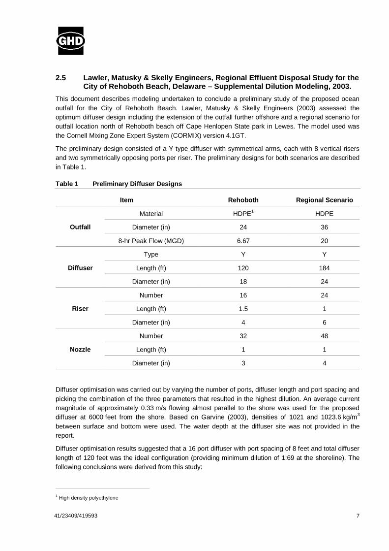
This document describes modeling undertaken to conclude a preliminary study of the proposed oceanoutfall for the City of Rehoboth Beach. Lawler, Matusky & Skelly Engineers (2003) assessed theoptimum diffuser design including the extension of the outfall further offshore and a regional scenario foroutfall location north of Rehoboth beach off Cape Henlopen State park in Lewes. The model used wasthe Cornell Mixing Zone Expert System (CORMIX) version 4.1GT.
The preliminary design consisted of a Y type diffuser with symmetrical arms, each with 8 vertical risersand two symmetrically opposing ports per riser. The preliminary designs for both scenarios are describedin Table 1.
Table 1 Preliminary Diffuser Designs
Item Rehoboth Regional Scenario
Outfall
Material HDPE1 HDPE
Diameter (in) 24 36
8-hr Peak Flow (MGD) 6.67 20
Diffuser
Type Y Y
Length (ft) 120 184
Diameter (in) 18 24
Riser
Number 16 24
Length (ft) 1.5 1
Diameter (in) 4 6
Nozzle
Number 32 48
Length (ft) 1 1
Diameter (in) 3 4
Diffuser optimisation was carried out by varying the number of ports, diffuser length and port spacing andpicking the combination of the three parameters that resulted in the highest dilution. An average currentmagnitude of approximately 0.33 m/s flowing almost parallel to the shore was used for the proposeddiffuser at 6000 feet from the shore. Based on Garvine (2003), densities of 1021 and 1023.6 kg/m3
between surface and bottom were used. The water depth at the diffuser site was not provided in thereport.
Diffuser optimisation results suggested that a 16 port diffuser with port spacing of 8 feet and total diffuserlength of 120 feet was the ideal configuration (providing minimum dilution of 1:69 at the shoreline). Thefollowing conclusions were derived from this study:
1 High density polyethylene

8 41/23409/419593Ocean Outfall PermittingAssessment of the Performance of the Rehoboth Beach Ocean Outfall
Modification of port spacing or the total number of ports did not significantly improve dilution and sincethe preliminary diffuser design was based on generally accepted principles balancing dilution andcosts, the preliminary design was deemed acceptable for the combination of effluent discharge andambient conditions at the site;
An assessment to check the relative benefit of locating the outfall to either 9000 or 12000 feet(compared with the initially proposed 6000 feet) demonstrated that the distance to achieve 1:100dilution is not improved. While not explicitly indicated in the report, this may be because of therelatively similar current magnitudes at these three locations. It was also concluded that while therewas no relative improvements in dilutions, extending the outfall may provide an additional margin ofsafety by allowing more time for decay. The downside would be that such outfall lengths wouldincrease head losses. [This uncertainty provides one of the reasons for undertaking far fieldmodeling.]
A dilution of 1:100 was expected to be achieved within 500 feet of the diffuser for the Regionalscenario and this mixing was considered to be adequate;
The modeling exercise used average tidal currents compared to subtidal (small) currents used in thepreliminary exercise. The use of average currents was considered more appropriate as the currents inthe Delaware coast are principally tidal. Dilution of 1:100 was achieved within 500 feet of the outfallfor average currents; and finally
The report noted that Garvine (2003) showed that both the horizontal and vertical variability of thecurrent field are high. Eddies of approximately 5 km in diameter surround the alternative diffuserlocations for Rehoboth Beach and the Regional solution. These current fields were not simulated inthe CORMIX model but are expected to further disperse the plume and limit its contact with theshoreline.
2.6 State of Delaware Surface Water Quality Standards, DNREC 2004Delaware’s bacterial water quality criterion requires for primary and secondary contact recreationalmarine waters the following values not to be exceeded
Contact Type Single-Sample Value(Enterococcus Colonies/100 ml)
Geometric Mean (EnterococcusColonies/100 ml)
Primary 104 35
Secondary 520 175
The criteria apply to enterococcus bacteria determined by the Department to be of non-wildlife originbased on best scientific judgement using available information.
941/23409/419593
2.7 Key FindingsKey findings from the literature review are summarised as follows:
Three frequency ranges (tidal, sub-tidal and low sub-tidal) are present in the current field at theproposed outfall site;
Comprehensive analysis must be carried out on a long-term basis to include the effects of seasonalclimatic changes as well as those of the rhythmic tidal fluctuations and variable inflow of freshwater;
Major forces driving the formation of currents and the mixing processes along the coast at Rehobothbeach include the tides, winds, freshwater inflows and density variations;
Using observed (rather than synthetic) tidal elevations at the offshore boundaries of the model (if suchdata exist) has the potential to yield good agreement between model predictions and observations;and
The duration of mixing processes during the tidal cycle is expected to be of the order of 1 hour as aminimum.
It should be noted that USEPA (1984) classifies the Delaware Bay as a vertically homogenous waterbody, that is, non-stratified and subjected to a small river discharge. The well-mixed nature of theDelaware River estuary is attributed to the fact that the estuary is generally shallow with a large tidalamplitude to depth ratio such that mixing can easily penetrate throughout the water column.
A rough estimate of the Richardson number – the primary parameter used to classify the stratificationpotential of an estuary yields a value of Ri=0.07 which is also an indication of well mixed conditions in theestuary (Ri<0.08).
Richardson number has been estimated with fQ = 5000 m3/s, W = 18000 m and tU = 1 m/s using the
following relationship:
3t
f
WUgQ
Ri ,
where is the difference between freshwater and seawater density, typically 25 kg/m3; is the
reference density, typically 1000 kg/m3; g is gravity (m/s2), fQ is the freshwater inflow (m3/s); W is the
width of the estuary (m); and tU is the mean tidal velocity (m/s). If Ri is large (>0.8), the estuary is
expected to be strongly stratified and dominated by density currents, and if Ri is small (<0.08), theestuary is expected to be well mixed. Transition from a well-mixed to a strongly mixed estuary occurs inthe range 8.008.0 Ri .
It is noted that the above estimate of Ri is conservative. Average freshwater inflow of the Delaware River(Whitney and Garvine 2006) is 570 m3/s and a typical high river discharge occurring during the springperiod is of the order of 1100 m3/s while the Delaware estuary is 18 km wide only at the mouth betweenCape Henlopen and Cape May. Accordingly, Ri is expected to be significantly less than 0.07.
As discussed in the subsequent sections of this report, the presence of well-mixed conditions in theDelaware estuary lends support to the primary adoption of a two-dimensional, depth-averaged frame ofanalysis for the project. Well-mixed conditions also facilitate effluent dilution.

10 41/23409/419593Ocean Outfall PermittingAssessment of the Performance of the Rehoboth Beach Ocean Outfall
3. Project Data
Data for the modeling component of the project comprises USGS and NOAA hydrographic andmeteorological datasets, depth soundings retrieved from the C-MAP bathymetric database integratedinto the DHI Mike suite of models, field data from a long-term monitoring campaign and six short-termintensive periods of measurement.
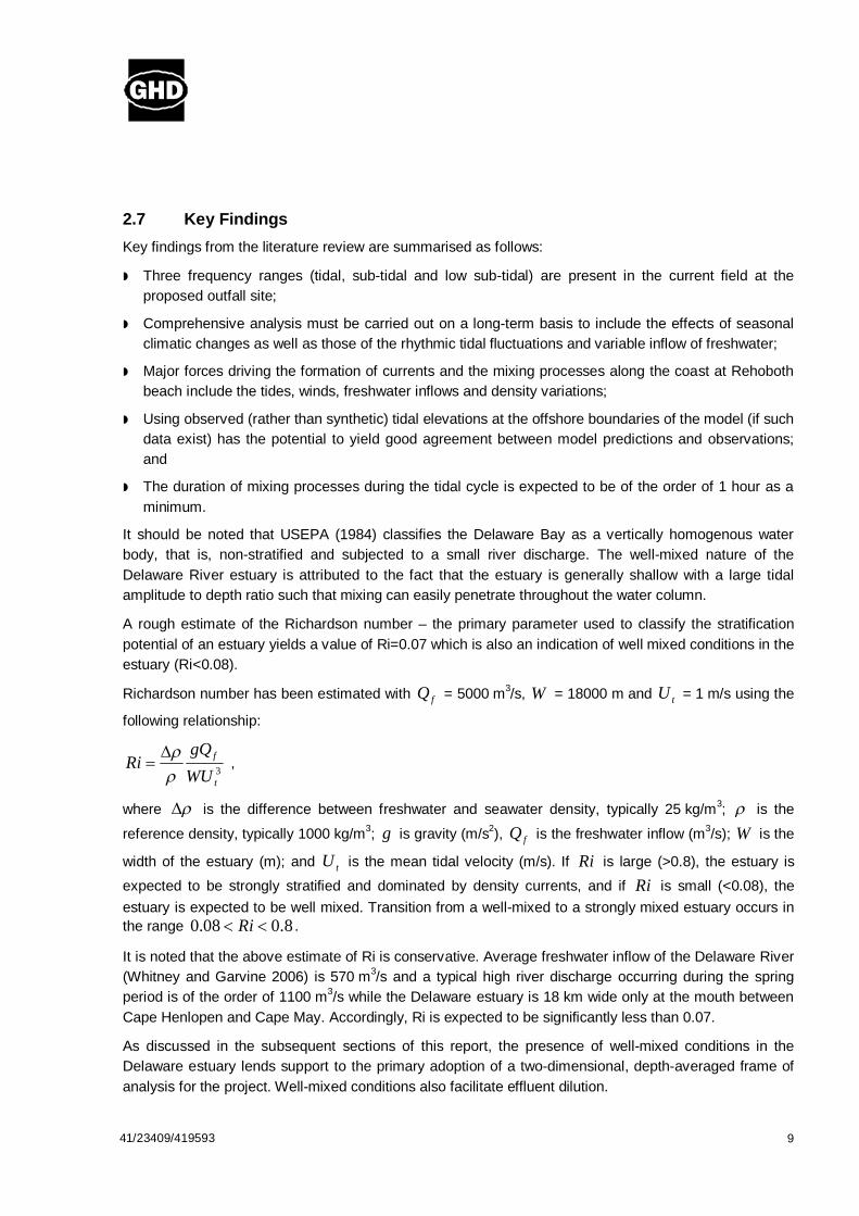
3.1 Short-Term Intensive SurveysThe short-term intensive surveys were one-day measurements of conductivity and temperature usingCTD instrumentation operated from a vessel. A CTD is an instrument that is lowered by a cable in thewater and measures the conductivity and temperature at a given water depth. A CTD has three probes.One is a ceramic probe that measures the conductivity, a thermistor that measures the temperature, anda pressure gauge that measures the ambient water pressure. The temperature and conductivity are usedto compute the water’s salinity (Encyclopedia of Marine Science, 2009).
In total, six short-term intensive surveys were undertaken at the locations shown in Figure 3-1. Thesurveys, undertaken to examine seasonal variation of density in the water column, proceed sequentiallyalong the three transects shown in the figure and include a varying number of individual measurements(17 on average). The vertical profiles of salinity, temperature and density, plotted in Appendix B, revealthat:
In November 2010 and January 2011, temperature between the surface and the deepest recordingsfluctuated (at most) 1 degree Celsius. However, March 2011 data suggests that temperatures mayvary by as much as a 3 degrees Celsius. Similarly with salinity, in November profiles fluctuated onlyabout 2 practical salinity units (psu) and in January 1 psu but in the March data salinity fluctuatedbetween approximately 20-21 psu at the surface and 30 psu at the deepest records. This is avariation of 10 psu compared to 1 or 2 previously. With density the increase is also substantial goingfrom a fluctuation of only 2 kg/m3 in November and January to a fluctuation of 10 kg/m3 in March.
The May 2010 observations were similar to the March ones. Maximum temperature differencebetween the surface and the deepest recordings varied up to 4 degrees Celsius while generally adifference of 1-2 degrees was recorded in depths similar to the ones associated with the proposedoutfalls. The maximum salinity and density differences between the surface and the deepestrecordings were 10 psu and 10 kg/m3, however the differences were of the order of 1 psu and lessthan 1 kg/m3 in depths similar to the ones associated with the proposed outfalls.
During the July 2011 short-term survey, the maximum temperature difference (between surface andbottom) in the vicinity of the proposed outfalls reached 3.5 degrees Celsius (stations R2 and R11) butsalinity difference did not exceed 1 psu thus the maximum recorded density difference was also low –approximately 1.5 kg/m3.
The September 2011 survey produced records were similar to the first two (November 2010 andJanuary 2011) with maximum temperature difference in the vicinity of the proposed outfalls of lessthan 1.0 degrees Celsius and maximum salinity and maximum density of less than 2 psu and2.0 kg/m3 respectively.
Overall, it appears that there is a relative increase in stratification at the deepest monitoring locationsduring March, May and July 2011 compared to the results obtained in November 2010, January and
1141/23409/419593
September 2011. This is mainly due to changing temperatures, the warming of surface waters and afreshwater lens impacting the surface waters. However, as observed, these effects are significantlyless pronounced in depths shallower than 15 m where the outfall is proposed to be built, hence, onthe basis of the short term surveys documented in this section, the assumption of well-mixedconditions holds true.
Figure 3-1 Field Data Collection Locations and Survey Transects
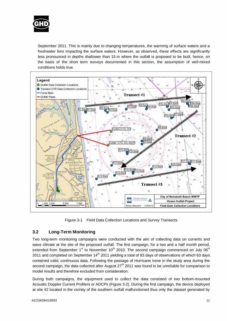
3.2 Long-Term MonitoringTwo long-term monitoring campaigns were conducted with the aim of collecting data on currents andwave climate at the site of the proposed outfall. The first campaign, for a two and a half month period,extended from September 1st to November 10th 2010. The second campaign commenced on July 06th
2011 and completed on September 14th 2011 yielding a total of 83 days of observations of which 63 dayscontained valid, continuous data. Following the passage of Hurricane Irene in the study area during thesecond campaign, the data collected after August 27th 2011 was found to be unreliable for comparison tomodel results and therefore excluded from consideration.
During both campaigns, the equipment used to collect the data consisted of two bottom-mountedAcoustic Doppler Current Profilers or ADCPs (Figure 3-2). During the first campaign, the device deployedat site #2 located in the vicinity of the southern outfall malfunctioned thus only the dataset generated by
12 41/23409/419593Ocean Outfall PermittingAssessment of the Performance of the Rehoboth Beach Ocean Outfall
the ADCP deployed at site #1 (near the proposed northern outfall) was made available for visualisationand analysis. The loss of the data from the second instrument precluded any measurements of thespatial characteristics of the velocity field at the outfall site as well as the possibility of conducting sanitychecks on the obtained records.
During the second campaign, both instruments functioned properly thus capturing the spatial distributionof flow in the area of interest and providing concurrent records at both potential outfall sites.
Figure 3-2 ADCP Deployment Locations
1341/23409/419593
ADCPs are designed to measure current velocity and direction at discrete intervals through the watercolumn but can also measure significant wave height, peak wave period and direction when waveenabled. All ADCP instruments deployed in the study area were wave enabled.
It should be noted that the current is measured throughout the water column in a series of depth cells or“bins” which are nominally of equal length and equally spaced. The measured currents are averagedover the range of each bin. The number of bins and the depth of the bins can be chosen by the operatorto suit the site conditions and to provide the required degree of vertical resolution.
During the first (2010) campaign, data for site #1 was collected in 21 bins at 0.5 m depth increments withthe first and last bins set at 1.5 m and 11.5 m above the bottom, respectively. The average depth at thesite was estimated at 11.5 m below MSL.
During the second (2011) campaign, data for both sites was collected at a similar vertical resolution, i.e.19 bins at site #1 and 20 bins at site #2. The average depth at site #1 was estimated at 12.2 m and theaverage depth at site #2 was estimated at 12.8 m.
In the remaining of this section, we further review and discuss the ADCP data collected during the firstfield campaign noting that the ADCP data collected during the second, 2011 campaign exhibit verysimilar characteristics to those of the data obtained during the first campaign as outlined in section 4.8 onmodel validation.
Three different techniques have been adopted in the visualisation of the ADCP data (Figure B-2 ofAppendix B). The techniques - frequency histograms, tidal orbits and the conventional time-series,substantially complement each other. For instance, frequency histograms make it possible to quantifyeven minor changes in current magnitude and direction occurring in each bin owing to the adoption offrequency analysis. Alternatively, tidal orbits and time-series tend to provide the best correlation betweenchanges in current magnitude and corresponding shifts in current direction.
As seen from Figure B-2 of Appendix B, the currents in all vertical bins (as defined by the directionalfrequency histograms) sit mainly in the alongshore direction defined as 360° and 180° True North whilethe offshore component of the currents is a minor contributor as the 330° and 150° directional binsindicate, never lasting more than 25% of the time in total. It is worth noting that for the period ofmeasurements during the first campaign (01 September to 10 November 2010) alongshore currentsheaded north for a maximum of 35% of the time with the remaining balance headed south.
A review of the frequency histograms for current magnitude from Figure B-2 indicates that with respect toalongshore currents:
– Near the bottom, the most frequently encountered current magnitude (alongshore currents) is inthe 0.3 to 0.4 m/s range for 47% of the time;
– In the first, bottom bin current magnitudes (alongshore currents) in the 0.3 m/s range dominate;
– Near the sea surface the distribution of current magnitude gradually shifts towards the 0.5 m/scurrent magnitude bin with magnitudes of this order observed less than 20% of the time;
– Current magnitudes exceeding 0.55 m/s have been encountered approximately 20% of the time orless.
An indication of the magnitude of the cross-shore currents is gained from the polar plots. Cross-shorecurrents are observed to remain under 0.1 m/s and are mostly uniformly distributed throughout the waterdepth. Occasional spikes have occurred near the surface that reach 0.15-0.20 m/s.

14 41/23409/419593Ocean Outfall PermittingAssessment of the Performance of the Rehoboth Beach Ocean Outfall
Figures B-2r and B-2s corresponding to near-surface measurements (10 m and 10.5 m above bottom)have been excluded from consideration owing to suspected fouling of the ADCP records in these depthbins.
Some representative current magnitudes and their corresponding minimum percent of exceedance aresummarized in Table 2. These are read from the probability of exceedance curve for the second from thebottom depth bin shown in Figure B-2c of Appendix B and can be used as inputs for near-field modelingof mixing characteristics.
Table 2 Representative Current Magnitudes and Minimum Exceedance for the Period ofMeasurements
# Current Magnitude (m/s) Minimum Exceedance2.5 m above bottom
(% of time)
1 0.6 3
2 0.5 10
3 0.4 30
4 0.3 55
5 0.2 72
6 0.1 87
3.3 Meteorological DataWinds in the model are represented as time varying, spatially uniform forcing using wind data (magnitudeand direction) at 6 minute or 1 hour intervals obtained from three existing weather buoys in the studyarea. These are (Figure B-3, Appendix B):
Station LWSD1 - 8557380 - Lewes, DE (6 minute interval, 6 year record starting 2004)
Station CMAN4 - 8536110 - Cape May, NJ, (6 minute interval, 6 year record starting 2004) and
Station 44009 (LLNR 168) DELAWARE BAY 26 NM Southeast of Cape May, NJ44009, (1 hourinterval, 26 year record starting 1984) considered to represent inner shelf meteorological conditions.
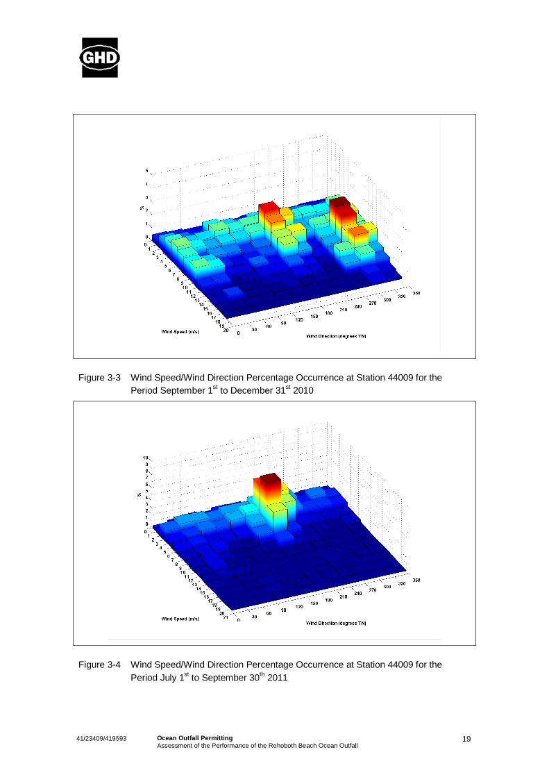
Wind statistics for station 44009 over a period of 5 months (August to December 2010), including theperiod during which the first long-term monitoring campaign was carried out (September 1st to November10th 2010), are presented in Table 3 and Table 4 and visualised in Figure 3-3. Monthly wind roses arealso provided in Appendix B.
For the nominated period (August to December 2010), the interpretation of the results using Table 4 andeach respective wind rose indicates that:
During the months of August and September, the prevailing winds were blowing from the SSW (180ºto 210º);
A relatively even distribution characterised the month of October. Directions from which the winds

1541/23409/419593
were blowing were spread between the NE (30º to 60º), the SW (210º to 240º) and the NW (300º to330º);
During the months of November and December, the prevailing winds were from the NW and NNW(300º to 360º) and NNE (0º to 30º) sectors.
Using Table 3 and Figure 3-3, it is observed that for the nominated period, winds blowing from the SSW(180º to 210º) and NW (300º to 330º) had the highest percentage of occurrence. Winds blowing from theNNE and NE direction were dominant during the month of November. The latter wind directions are ofparticular interest in this study since the winds blowing from these directions are likely to have an impacton the water quality near the coast.
Wind statistics for station 44009 over a period of 3 months (July, August and September 2011), includingthe period during which the second long-term monitoring campaign was carried out (July 6th toSeptember 14th 2011) are shown in Figure 3-4. As indicated from the figure, the prevailing winds for thisperiod were blowing from the SSW (180º to 210º). There were no winds from the NW quadrant for theperiod.
Also summarised in Figure 3-5 for comparative purposes are the wind statistics for the first half of 2011.While the dominance of winds blowing from the SSW (180º to 210º) is still clearly observed, acontribution from winds from the NNW (330º to 360º) sector is also evident for the period.
As noted in the following sections, provisions have been made to represent the seasonal variability of thewind (and hence wave) climate (as illustrated by the above figures) in the effluent plume analysis byconducting the latter over a period of 11 months.

41/23409/41959316
Table 3 Wind Statistics – Wind Speed/Wind Direction at Station 44009 for the Period August 1st to December 31st 2010
WindSpeed(m/s)
Wind Direction True North (degrees)
0 ~<30
30 ~<60
60 ~<90
90 ~<120
120 ~<150
150 ~<180
180 ~<210
210 ~<240
240 ~<270
270 ~<300
300 ~<330
330 ~<360
Total
0 ~ <1 0.08% 0.11% 0.14% 0.03% 0.03% 0.08% 0.16% 0.08% 0.03% 0.08% 0.08% 0.11% 1.01%
1 ~ <2 0.54% 0.52% 0.33% 0.49% 0.25% 0.49% 0.38% 0.30% 0.35% 0.14% 0.16% 0.33% 4.28%
2 ~ <3 0.54% 0.44% 0.33% 0.79% 0.74% 0.49% 0.84% 0.82% 0.52% 0.71% 0.44% 0.41% 7.05%
3 ~ <4 0.65% 0.52% 0.54% 1.03% 0.76% 0.74% 0.63% 0.76% 0.74% 0.71% 0.74% 0.65% 8.47%
4 ~ <5 1.12% 0.68% 0.87% 0.71% 0.87% 1.06% 1.42% 1.66% 0.65% 0.90% 0.71% 1.12% 11.76%
5 ~ <6 0.87% 0.82% 0.54% 0.71% 0.60% 0.76% 1.99% 1.03% 0.68% 0.63% 0.57% 1.09% 10.29%
6 ~ <7 0.65% 0.44% 0.68% 0.60% 0.33% 0.60% 1.36% 0.54% 0.49% 0.87% 0.82% 0.82% 8.20%
7 ~ <8 1.28% 0.27% 0.38% 0.25% 0.35% 0.22% 1.44% 1.12% 0.63% 0.65% 1.39% 1.42% 9.40%
8 ~ <9 0.60% 0.71% 0.27% 0.19% 0.33% 0.33% 1.12% 1.31% 0.22% 0.65% 2.12% 1.12% 8.96%
9 ~ <10 0.71% 0.71% 0.25% 0.16% 0.30% 0.30% 1.25% 0.60% 0.25% 0.65% 1.93% 0.95% 8.06%
10 ~<11 0.76% 0.76% 0.05% 0.19% 0.38% 0.19% 0.68% 0.35% 0.08% 0.41% 1.61% 0.87% 6.35%
11 ~<12 0.30% 0.27% 0.00% 0.08% 0.19% 0.22% 0.35% 0.30% 0.08% 0.38% 1.17% 1.31% 4.66%
12 ~<13 0.05% 0.11% 0.03% 0.00% 0.03% 0.22% 0.14% 0.22% 0.03% 0.65% 1.33% 0.98% 3.79%

1741/23409/419593
WindSpeed(m/s)
Wind Direction True North (degrees)
0 ~<30
30 ~<60
60 ~<90
90 ~<120
120 ~<150
150 ~<180
180 ~<210
210 ~<240
240 ~<270
270 ~<300
300 ~<330
330 ~<360
Total
13 ~<14 0.08% 0.16% 0.00% 0.00% 0.05% 0.03% 0.16% 0.08% 0.00% 1.20% 1.69% 0.46% 3.92%
14 ~<15 0.08% 0.30% 0.00% 0.00% 0.03% 0.11% 0.00% 0.03% 0.00% 0.49% 0.95% 0.46% 2.45%
15 ~<16 0.05% 0.08% 0.00% 0.00% 0.00% 0.03% 0.00% 0.00% 0.00% 0.03% 0.19% 0.16% 0.54%
16 ~<17 0.00% 0.00% 0.00% 0.00% 0.00% 0.00% 0.00% 0.00% 0.00% 0.00% 0.33% 0.14% 0.46%
17 ~<18 0.00% 0.00% 0.00% 0.00% 0.00% 0.00% 0.00% 0.00% 0.00% 0.00% 0.16% 0.14% 0.30%
18 ~<19 0.00% 0.00% 0.00% 0.00% 0.00% 0.00% 0.00% 0.00% 0.00% 0.00% 0.05% 0.00% 0.05%
Total 8.39% 6.89% 4.41% 5.23% 5.23% 5.86% 11.93% 9.20% 4.74% 9.15% 16.45% 12.53% 100.00%
18 41/23409/419593Ocean Outfall PermittingAssessment of the Performance of the Rehoboth Beach Ocean Outfall
Table 4 Wind Statistics – Monthly Wind Direction at Station 44009 for the Period August to December 2010
Wind Direction (degrees) August September October November December Total
0 ~ <30 1.39% 1.93% 0.84% 3.02% 1.20% 8.39%
30 ~ <60 1.25% 1.50% 2.15% 1.83% 0.16% 6.89%
60 ~ <90 1.47% 0.63% 1.36% 0.71% 0.25% 4.41%
90 ~ <120 1.96% 0.98% 0.54% 1.50% 0.25% 5.23%
120 ~ <150 1.44% 1.23% 0.38% 1.44% 0.74% 5.23%
150 ~ <180 1.69% 2.29% 0.38% 1.12% 0.38% 5.86%
180 ~ <210 3.54% 4.11% 2.56% 0.95% 0.74% 11.90%
210 ~ <240 2.75% 1.77% 2.75% 1.25% 0.68% 9.21%
240 ~ <270 1.17% 0.68% 1.99% 0.57% 0.33% 4.74%
270 ~ <300 0.98% 0.93% 2.59% 1.31% 3.35% 9.15%
300 ~ <330 0.79% 1.63% 2.94% 2.72% 8.36% 16.45%
330 ~ <360 1.83% 1.93% 1.77% 3.19% 3.81% 12.53%
Total 20.27% 19.61% 20.27% 19.61% 20.24% 100.00%
1941/23409/419593 Ocean Outfall PermittingAssessment of the Performance of the Rehoboth Beach Ocean Outfall
Figure 3-3 Wind Speed/Wind Direction Percentage Occurrence at Station 44009 for thePeriod September 1st to December 31st 2010
Figure 3-4 Wind Speed/Wind Direction Percentage Occurrence at Station 44009 for thePeriod July 1st to September 30th 2011

20 41/23409/419593Ocean Outfall PermittingAssessment of the Performance of the Rehoboth Beach Ocean Outfall
Figure 3-5 Wind Speed/Wind Direction Percentage Occurrence at Station 44009 for thePeriod January 1st to June 30th 2011
3.4 Wave DataWave data has been obtained from Station 44014 (LLNR 550) VIRGINIA BEACH 64 NM Eastof Virginia Beach, VA, (1 hour interval, 30 year record starting 1980) and consisted of significantwave height, spectral peak wave period and mean wave direction.

2141/23409/419593 Ocean Outfall PermittingAssessment of the Performance of the Rehoboth Beach Ocean Outfall
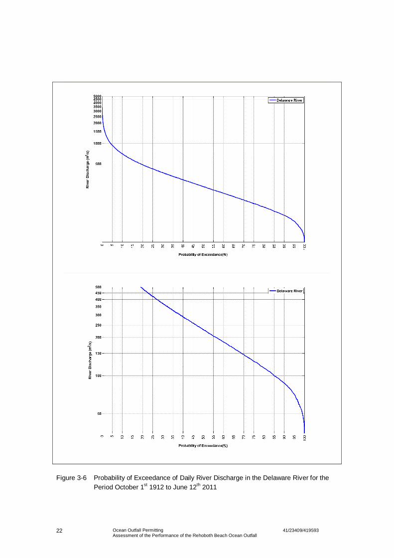
3.5 Freshwater InflowsAs indicated above, the Delaware River above Trenton, New Jersey, providing 58% of thefreshwater flowing into the Delaware Bay according to Sharp (1984), is used as one of themajor forces to drive the simulation. Freshwater inflows included in the analysis have beenrepresented using the U.S. Geological Service daily river discharge record at Trenton for the2010 period applied approximately 165 km upstream from Cape Henlopen near Bellefonte andadjusted to account for additional sources of freshwater (refer section 4.7.2 for details).
A probability of exceedance curve for the daily river discharge has been derived from the entireset of observations at the nominated location (October 1st 1912 to June 12th 2011). The curve,shown in Figure 3-6, indicates the probability that a daily Delaware river discharge, shown onthe vertical axis of the graph, will be exceeded at the location. As determined from the curveand on the basis of approximately a century-long period of observations, a river discharge of1000 m3/s is expected to be exceeded 4% of the time, a river discharge of 500 m3/s is expectedto be exceeded 19% of the time and so on.
Using the curve given in Figure 3-6, one can determine the probability of exceedance of theDelaware river discharge recorded during the period of each of the short-term intensive surveysdescribed in section 3.1 and, in association with the conditions measured at the outfall area,establish a correlation between river discharge probability and the probability of encounteringvertical stratification in the area of the proposed outfall. This is a valid approach since verticalstratification in the water column has been found to be directly associated with periods of highinflows from the Delaware river (refer section 2.3). Following the described approach, the dailydischarges corresponding to the 2010-2011 surveys which were associated with some degreeof stratification at the outfall are identified in columns 3 of Table 5 and observed (column 4) tohave a relatively low probability of exceedance of 2-6%.
While a larger sample of paired river discharge and short-term intensive measurements isnecessary to improve the reliability of this estimate, a less than 6% probability of exceedance ofthe daily discharges associated with some degree of stratification imply that the probability ofstratified conditions developing at the outfall site and caused by river inflows is also relativelylow.
In addition, following the methodology presented in section 2.7, all river discharges listed inTable 5 are associated with well-mixed conditions in the Delaware estuary (values of Ri of lessthan 0.08).
It should be noted that all discharges included in the above analysis have been lagged by 14days to allow for the time it approximately takes for a flow discharge measured at Trenton toreach the study area.
22 41/23409/419593Ocean Outfall PermittingAssessment of the Performance of the Rehoboth Beach Ocean Outfall
Figure 3-6 Probability of Exceedance of Daily River Discharge in the Delaware River for thePeriod October 1st 1912 to June 12th 2011

2341/23409/419593 Ocean Outfall PermittingAssessment of the Performance of the Rehoboth Beach Ocean Outfall
Table 5 Short-term Intensive Surveys - Measured Daily River Discharge, AssociatedProbability of Exceedance and Receiving Water Condition
Survey#
Date Measured DailyRiver Discharge(m3/s)
Probability ofExceedance(%)
StratifiedConditions
1 November 18th 2010 285.4 33.5 Low
2 January 25th 2011 194 67.5 Low
3 March 17th 2011 1163 2.2 Low tomoderate
4 May 25th 2011 738 5.8 Low tomoderate
5 July 11th 2011 1112 3.3 Low tomoderate
6 September 14th 2011 2773 0.2 Low tomoderate
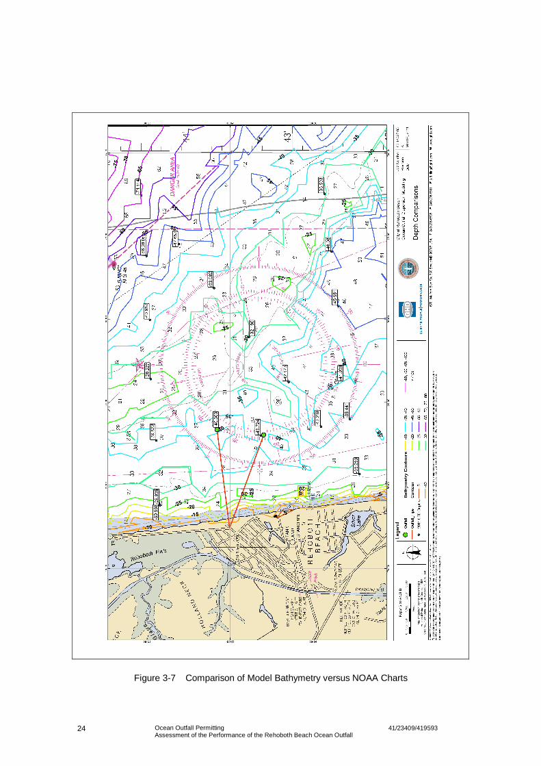
3.6 BathymetryDepth measurements for modeling purposes off the coast of Rehoboth Beach were obtainedfrom multiple sources. Primarily, the coastline and bathymetric data were obtained from the C-Map database (Jeppesen) and NOAA. Bathymetric data was also collected during the six shortterm surveys.
Another source of depth measurements comprised cross-shore profiles generated by the U.S.Army Corp of Engineers. This data only extends a few hundred feet offshore and was not usedin the analysis. However, it is expected to play an important role during the design stage of theproposed outfall.
As demonstrated from Figure 3-7, there is a good agreement between model bathymetry(coloured contours) and the underlying NOAA chart. All key bathymetric features offshore ofRehoboth Beach are rendered in the model.
Additional bathymetric features (at different scales) can also be observed in Figure 4-1 andFigure 4-2.
24 41/23409/419593Ocean Outfall PermittingAssessment of the Performance of the Rehoboth Beach Ocean Outfall
Figure 3-7 Comparison of Model Bathymetry versus NOAA Charts

2541/23409/419593 Ocean Outfall PermittingAssessment of the Performance of the Rehoboth Beach Ocean Outfall
4. Model Establishment and Calibration
4.1 IntroductionThe usefulness of numerical hydrodynamic-transport and water quality models as powerful toolsfor impact assessment studies has long been recognized, with methodologies for their rigorousimplementation well established (STOWA 99-05). Flow and transport are integrally linked,meaning that accurate quantification of the time- and space-varying flow conditions of thereceiving waters is required to accurately evaluate the transport of waterborne constituents. Nettrends in transport, which may vary on a seasonal basis, must also be properly captured andadequately incorporated into the analysis of the ultimate fate of the effluent.
To ensure that the identification of potential impacts from the proposed works is carried out inan effective manner whilst protecting sensitive habitats and recreational areas, a soundunderstanding of the dominant physical forces and processes in the coastal area of interest isessential. The acquired knowledge is then synthesized in a numerical model capable ofproviding a quantitative description of circulation patterns, flushing characteristics and transporttrends as well as answers to what-if scenarios which are fundamental to the impact assessmentprocess.
The following sections provide a description of the hydrodynamic and transport modelingsystem developed for the assessment of the plume dispersion processes at Rehoboth Breach.
4.2 Governing EquationsThe modeling system adopted for the Rehoboth Beach outfall study is applicable to scalesranging from estuaries to regional ocean domains. In its current application, it simulates two-dimensional, depth-averaged or three-dimensional non-linear, unsteady flow and transportphenomena resulting from the effects of the tide, waves, winds, freshwater inflows, density andthe effects of the earth’s rotation. Density effects are due to time (seasonally) and spatiallyvarying (non-uniform) temperature and salinity distributions.
The modeling process is based on a system of standard equations comprising:
The incompressible Reynolds-averaged Navier-Stokes (or RANS) equations describing theconservation of momentum and mass in a Cartesian coordinate system rotating with theearth and subject to the hydrostatic pressure and Boussinesq assumptions;
Two advection-diffusion equations for the transport of salinity and temperature; and
The state equation.
It is noted that:
The fluid is assumed to be incompressible. Accordingly, the density does not depend onthe pressure but only the temperature T and the salinity S via the equation of state in theform = (T,S); and
Use is made of the UNESCO equation of state.
The prognostic variables are the free surface elevation and the two components of transport orvelocity. The spatial discretization of the primitive equations is performed using a cell-centred
26 41/23409/419593Ocean Outfall PermittingAssessment of the Performance of the Rehoboth Beach Ocean Outfall
finite-volume method. In two-dimensional mode, the one adopted for the current analysis, thespatial domain is represented on a flexible (unstructured) mesh of non-overlapping triangular orquadrilateral elements.
Turbulence is modelled using an eddy viscosity concept with sub-grid scale transportsrepresented by an effective eddy viscosity related to a characteristic length scale. Thisformulation, introduced by Smagorinsky, represents turbulence at scales smaller than the modelmesh size.
The hydrodynamic model is an implementation of Mike 21 Flexible Mesh module integrated inthe Danish Hydraulic Institute (DHI) suite of models.
Sharing the unstructured mesh of the hydrodynamic model is a fully spectral wind-wave modelbased on the wave action conservation equation. The wave model has been developed tocalculate the growth, decay and transformation of wind-generated waves in the study and is animplementation of Mike 21 SW with the discretization of the governing equation in spectralspace performed using a cell-centred finite volume method while the time integration isperformed using an explicit fractional step approach (Mike 21 SW User’s manual).
4.3 Model DomainThe simulation domain (Figure 4-1) includes the entire Delaware estuary and 375 km of theadjacent continental shelf extending some 105 km offshore to maximum depths ofapproximately 100 m. The included section of continental shelf stretches from the mouth of theDelaware estuary 160 km north past Bamegat Bay reaching Point Pleasant Beach and 215 kmto the south ending at Cape Charles at the mouth of Chesapeake Bay.
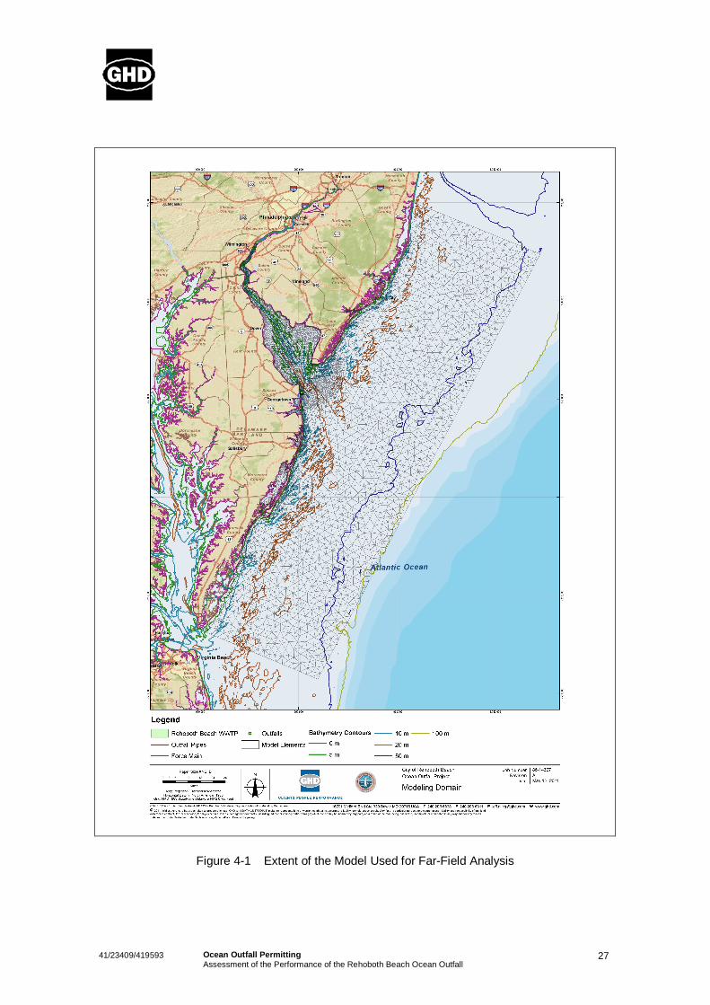
The model mesh contains 12730 elements and 7247 nodes with highest horizontal resolutionencountered near the outfall of the order of 160-200 m (Figure 4-2).
2741/23409/419593 Ocean Outfall PermittingAssessment of the Performance of the Rehoboth Beach Ocean Outfall
Figure 4-1 Extent of the Model Used for Far-Field Analysis
28 41/23409/419593Ocean Outfall PermittingAssessment of the Performance of the Rehoboth Beach Ocean Outfall
Figure 4-2 Magnified View of the Mesh of the Model at the Proposed Outfall Site
2941/23409/419593 Ocean Outfall PermittingAssessment of the Performance of the Rehoboth Beach Ocean Outfall
4.4 Model OperationThe model was operated in a two-dimensional, depth-averaged mode for calibration andvalidation purposes as well as for long-term (one-year duration) operational runs. The adoptedtwo-dimensional formulation implies that stress terms are applied only at the surface (windeffects) and at the sea bed as bottom friction.
Two field data collection campaigns were organised during the course of the project thatprovided independent datasets needed to support the calibration and validation of the model.Calibration was carried out against the first dataset (2010). The second dataset (2011) wasused for model validation.
4.5 Forcing of the Hydrodynamic ModelThe primary forcing factors included in the analysis are: tides, winds, waves, Delaware Riverdischarge and, in the case of a three-dimensional model, density effects as driven by seasonalchanges in salinity and temperature. Excluded from the model are heat transfer processesthrough the water surface, precipitation, evaporation and large-scale shelf circulation.
Tidal elevations are imposed along the offshore boundaries of the model by specifyingamplitude and phase for each of the following 8 major tidal constituents: Q1, O1, P1, K1, N2,M2, S2 and K2. These are obtained from the DHI global tidal model which is an integral part ofthe adopted modeling system.
4.6 Forcing of the Wave ModelThe wave model is forced by offshore winds applied to the free-surface of the model andoffshore open boundary conditions comprising significant wave height, spectral peak waveperiod, mean wave direction and a directional spreading index.
4.7 Model CalibrationThis section describes the model calibration process. The limitations of assumptions involved inthe calibration are also discussed. Calibration of the model to both predictions and fieldmeasurements is provided to demonstrate that the model is capable of simulating realisticallythe water elevations and currents at the outfall site over a prolonged period of time. Furtherconfirmation of the predictive capability of the model is provided by means of validation of themodel results against the second independent field dataset (refer section 4.8) and verification ofthe model results to previous work (section 4.9).
Model calibration is a process whereby model predictions are compared to field data consistingof measured water levels and currents in order to assess the predictive capability of the model.
NOAA’s tidal predictions for the Lewes station and field data collected offshore of Rehobothbeach during September to November 2010 have been used to calibrate the model.
The key parameter for model calibration is the bottom roughness coefficient. Mesh quality andresolution, coastal bathymetry and offshore boundary conditions also play a major role in thesuccessful calibration and, later on, operation of the model.
30 41/23409/419593Ocean Outfall PermittingAssessment of the Performance of the Rehoboth Beach Ocean Outfall
In total, 32 scenarios were investigated for calibration purposes. Modeling conditions included:
Tide only;
Tide and freshwater river inflow;
Tide and wind (several datasets described in section 3.3);
Tide, freshwater river inflow and wind; and
Tide, freshwater river inflow, wind and wave (dataset described in section 3.4).
Water elevation, current and wave measurements used for calibration of the modeling systemwere as recorded by the Acoustic Doppler Current Profiler or ADCP deployed near the southernleg of the outfall (38.730°N, 75.058°W) for the period 01 September 2010 to 10 November 2010(refer section 3.2 for details). For the purpose of calibration, the system was operated for aperiod of three months starting on 15th August 2010 thus including a two-week warm-up periodin the simulation.
Predictions of tidal elevation for the Lewes tidal station were also obtained for the 8 major tidalconstituents listed in the previous section and used in the process of calibration of the model totide.
4.7.1 Model Calibration to Predicted Tides
With respect to tides, the modeling system was calibrated against predictions of water surfaceelevation sourced from NOAA at Lewes tidal station, the closest to the project site. The resultsof the calibration, illustrated in Figures C-1 and C-2 presented in Appendix C, are quantitativelyanalysed in terms of the root-mean-square-error or RMSE. The RMSE is used herein as anobjective criteria for the assessment of the performance of the modeling system. Provided atime-series of observed iO and simulated iS values, RMSE is calculated as follows:
NSO
RMSE ii2
where N denotes the number of samples included in the statistical measure.
In terms of tidal elevation, a value of RMSE 0.1 m indicates that there is a good agreementbetween predicted and simulated tidal elevations.
A total of nine three-month simulations starting on 15th August 2010 were undertaken as part ofthe calibration process during which Manning’s roughness coefficient and tide-only, water leveloffshore boundary conditions (obtained from the DHI global tidal model) were graduallyadjusted. Logically, the simulation period for the calibration exercise was selected to coincidewith the period of the most recent field collection program (01 September to 10 November2010).
The lowest RMSE achieved in the above simulations was 0.06 m. These results (Figures C-1and C-2, Appendix C) were obtained for a Manning’s roughness coefficient of n=0.045, aSmagorinsky formulation of the horizontal eddy viscosity and slightly increased (with referenceto the global tidal model) tidal amplitudes at the offshore open boundaries of the model. A factor

3141/23409/419593 Ocean Outfall PermittingAssessment of the Performance of the Rehoboth Beach Ocean Outfall
of 1.2 applied uniformly across all open boundaries of the model was found to produce the bestmatch with NOAA’s predictions.
It is noted that global tidal models such as the one used to supply the offshore boundaryconditions for the present study use only the 8 major tidal constituents described in section 4.5.In order to preserve consistency in the analysis, all tidal predictions obtained from NOAA usethe same set of constituents.
A comparison of predicted and simulated tidal elevations (at tidal station Lewes) is presented inFigures C-1 and C-2 of Appendix C. In addition, Figures C-3 and C-4 of the appendix comparethe simulated tidal elevations at the proposed outfall site (site of deployment of ADCP#1) withthe NOAA predictions. With the exception of a minor phase lag that accounts for the distancethat the tide has to travel between the two locations, the comparison reveals little difference inthe predicted behaviour of the tide at the outfall site and station Lewes.
This is interpreted as an indication that:
In terms of tidal elevation, the quality of the obtained solution at the outfall site (as expressedby the level of agreement between tidal predictions and tide-only simulations) is good; and
Tidally-induced mixing processes are expected to be adequately represented in plumedispersion solutions.
4.7.2 Calibration to Tide, Winds, Waves and Freshwater Inflows (Time histories andpolar plots)
The process of calibration to currents involved:
Operating the system in two-dimensional mode using as input:
– the predicted tidal signal generated by the integrated global tidal model;
– wind fields (varying in time, constant in domain) reconstructed from hourly records of windspeed and direction obtained from station 44009 (LLNR 168) - Delaware Bay, 26 nauticalmiles Southeast of Cape May, NJ;
– wave climate (varying in time, constant along the offshore boundaries of the model)reconstructed from hourly records of significant wave height Hs (m), spectral peak waveperiod Tp (s), mean wave direction MWD (degrees true north) and directional spreadingindex n obtained from wave station 44014 (LLNR 550) - Virginia Beach, positioned 64nautical miles East of Virginia Beach, VA;
– daily freshwater inflows from the Delaware River obtained at station USGS 01463500Delaware River at Trenton NJ and multiplied by a factor of 1.5 to account for additionalsources of freshwater that enter the system downstream of Trenton;
Assessing the sensitivity of the solution to Manning’s roughness coefficient n. The coefficientwas varied in the 0.024 to 0.045 range;
Using a Smagorinsky formulation of the horizontal eddy viscosity; and
Averaging current direction and current magnitude ADCP records over depth.

32 41/23409/419593Ocean Outfall PermittingAssessment of the Performance of the Rehoboth Beach Ocean Outfall
The results of the calibration are presented in Figures C-5 to C-9 of Appendix C in the form of:
Time histories of measured and modelled water levels and a time history of thecorresponding residuals (measured water levels – modelled water levels), Figure C-5;
Time histories of measured and modelled (two-dimensional) current magnitude at the siteof deployment of the ADCP and a time history of the residual (measured current magnitude –modelled current magnitude), Figure C-6;
Polar plots of measured and modelled currents with the measured currents presented in twoways: (1) as a statistical mean and (2) a 95th percentile graph (Figure C-7);
Time histories of measured and modelled significant wave heights Hs (m), Figure C-8; and
Time histories of measured and modelled peak wave periods Tp (s), Figure C-9.
It is noted that:
All comparisons are referred to the site of deployment of ADCP #1 and have beenundertaken for the period of the measurements;
The residual water level time history shown in Figure C-5 has been obtained by subtractingmodelled from measured water levels over the period of the measurements;
Similarly, the residual current magnitude time history shown in Figure C-6 has been obtainedby subtracting modelled from measured current magnitudes for the period of themeasurements, with the measured current magnitudes averaged over the water column;
The polar plots in Figure C-7 allow a simultaneous assessment of modelled current directionand magnitude against two statistical representations of the measurements – the statisticalmean and the 95th percentile of current magnitude;
The 95th percentile representation of the currents while filtering major spikes in themeasurements (which the model cannot represent subject to the adopted forcing datasetsand modeling conditions) enhances significantly the comparison between model andmeasurements.
Following from the comparison in Figure C-5, it is observed that the difference betweenmodelled and measured water levels (or residual) at the outfall site could reach up to ±0.5 m forthe period of the measurements. From the comparison of current magnitudes, the estimateddifference is estimated to be of the order of ±0.25-0.30 m/s. The underlying assumption in theseestimates is that:
Events associated with a large residual have a low frequency of occurrence, hence littleimpact on transport trends; and
All measured physical entities (to which the model results are being compared to) are free ofsubstantial error due to data handling and/or operation of the instrumentation.
It is important to also note that a comparison of predicted and measured water levelsundertaken by NOAA at tidal station Lewes for the months of September, October andNovember 2010 (Figures C-10 to C-12 of Appendix C) estimates the maximum water levelresiduals for the three months at 0.5 m, 0.8 m and 0.7 m, respectively. While Lewes is adistance away from the proposed outfall site, the results highlight further the complexity of thehydrodynamic processes occurring in the study area.
3341/23409/419593 Ocean Outfall PermittingAssessment of the Performance of the Rehoboth Beach Ocean Outfall
As seen from Figures C-8 and C-9, the model matches well the observed significant waveheight and peak wave period for the period of the measurements. This is evidence that the windand wave data included in the modeling represent fairly well the wave climate along the coast ofRehoboth Beach. In addition, the good match of the measured wave heights and peak waveperiods is interpreted as evidence of the fact that both wind speed and direction, a major factorin the formation of local sea wave climate, are adequately represented in the modeling system.
4.7.3 Calibration to Tide, Winds, Waves and Freshwater Inflows (frequencyhistograms)
Comparison of ADCP records at 2.5 m above bottom and depth averaged model results (Figure4-3) has been carried out in terms of probability of exceedance of current magnitude, frequencyhistogram for current magnitude and frequency histogram for current direction. This has beenundertaken to assess the performance of the model in a statistical manner (with high relevanceto the process of regulatory mixing zone evaluation) rather than on the basis of individualrecords.
ADCP records at 2.5 m above bottom have been used in the comparison as bottom currents arelower than those near the surface (refer section 3.2) and as such will generate worse caseassessment scenarios.
As evidenced from Figure 4-3 the agreement between current measurements and model resultsis satisfactory in implying that near field analysis (drawing substantially from ADCP data) andmodel-based far-field analysis (verified against ADCP data) should be highly consistent. Thisstatement is made in terms of the applied forcing to plume formation in the near-field andadvection-diffusion in the far-field as well as throughout the assumptions adopted for theanalysis. In other words, no discontinuities associated with the applied forcing are anticipated tooccur in the modelling process, and hence in the final solution.
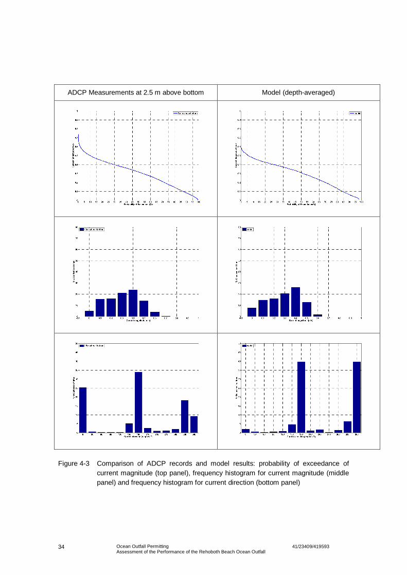
34 41/23409/419593Ocean Outfall PermittingAssessment of the Performance of the Rehoboth Beach Ocean Outfall
ADCP Measurements at 2.5 m above bottom Model (depth-averaged)
Figure 4-3 Comparison of ADCP records and model results: probability of exceedance ofcurrent magnitude (top panel), frequency histogram for current magnitude (middlepanel) and frequency histogram for current direction (bottom panel)
3541/23409/419593 Ocean Outfall PermittingAssessment of the Performance of the Rehoboth Beach Ocean Outfall
4.8 Model ValidationIn addition to calibration, the model was subjected to a process of validation which consisted ofrerunning the model for a different period of time (from the one adopted during the calibrationprocess) and comparing model results to both predictions and field measurements following thealready established procedure. The aim of the validation process was to confirm the predictivecapability of the model. This was done by obtaining a second set of predictions and comparing itagainst a dataset of observations not involved in the calibration process.
The results of the validation process are presented starting with Figure C-21 of Appendix C.Figures C-21 and C-22 show water levels (predicted using NOAA tidal constituents versusmodeled) at station Lewes for the month of July 2011. An RMSE value of 0.07 m has beenachieved over a period of the 63 days indicating that the quality of the prediction is very similarto the one achieved during the calibration process (0.06 m).
Figures C-23 and C-24 of the Appendix compare the simulated elevations in the vicinity of theproposed outfall site (site of deployment of ADCP #1) with the NOAA predictions and reveal thatthere is little difference in the predicted behaviour of the tide at the outfall and station Lewes.Similarly to the calibration results shown in Figures C-3 and C-4, a minor phase lag accounts forthe distance between the two locations (Lewes and the outfall site).
Validation to tide, winds, waves and freshwater inflows at the site of ADCP #1 deployed in thevicinity of the proposed northern outfall is illustrated in Figures C-25 to C-29 showing:
Time histories of measured and modelled water levels and a time history of thecorresponding residuals (measured water levels – modelled water levels), Figure C-25;
Time histories of measured and modelled (two-dimensional) current magnitude at the siteof deployment of the ADCP and a time history of the residual (measured current magnitude –modelled current magnitude), Figure C-26;
Polar plots of measured and modelled currents with the measured currents presented in twoways: (1) as a statistical mean and (2) a 95th percentile graph (Figure C-27);
Time histories of measured and modelled significant wave heights Hs (m), Figure C-28; and
Time histories of measured and modelled peak wave periods Tp (s), Figure C-29.
For the same period, the above sequence of graphs has been also generated for ADCP #2deployed in the vicinity of the proposed southern outfall. The corresponding figures in AppendixC are Figures C-30 to C-34.
Figures C-35 to C-38 illustrate the impact of Hurricane Irene on the data recorded by ADCP #2.As such, the data recorded after the 27th of August 2011, has been excluded from the analysis.
Finally, Figures C-39 to C-41 (directly comparable to C-10 to C-12 of Appendix C correspondingto the calibration period) present a comparison of predicted and measured water levelsundertaken by NOAA at tidal station Lewes for the months of July, August and September 2011and give estimates of the maximum water level residuals for the three months.
In summary, the results obtained during the process of model validation are found to bequalitatively and quantitatively consistent with the calibration results across all investigatedparameters. The predictive capability of the model is adequate for the intended purpose,namely, the prediction of the footprints of the plume transported by advection and dispersion.
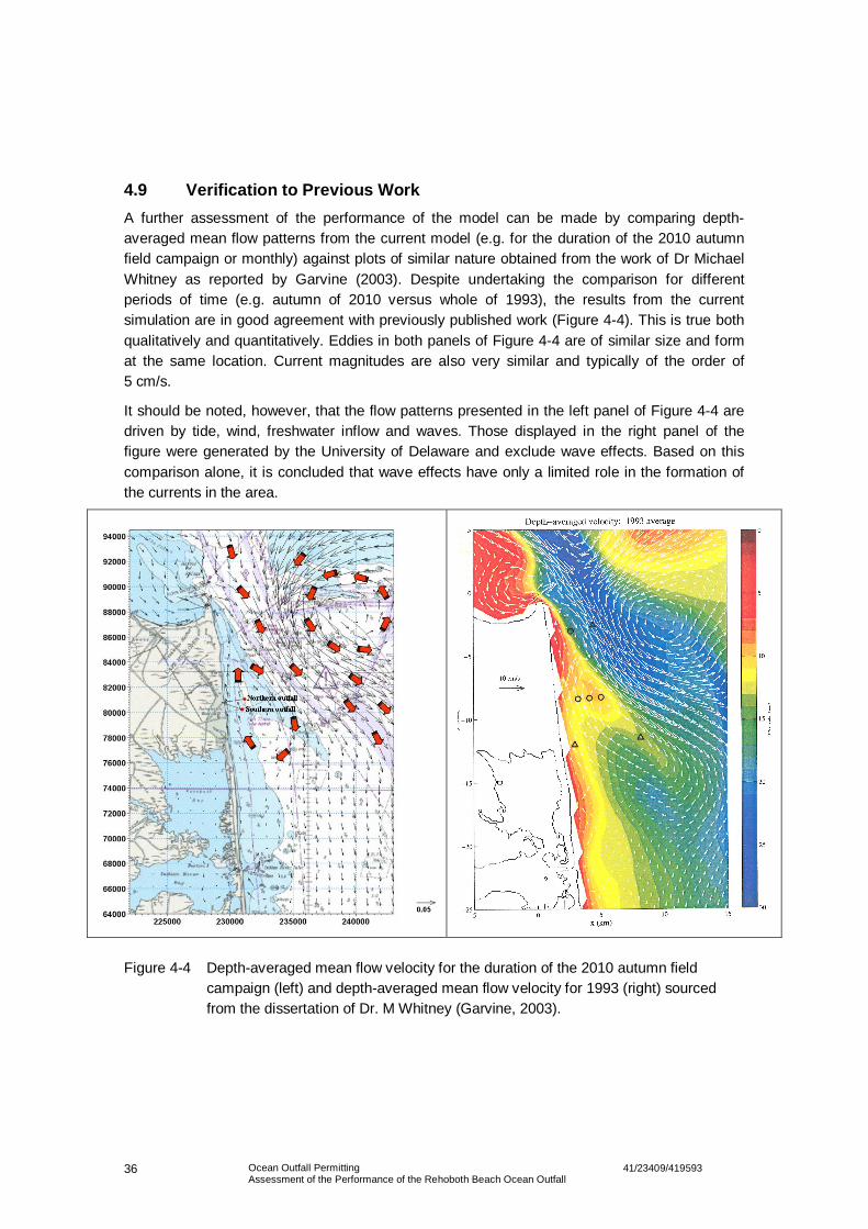
36 41/23409/419593Ocean Outfall PermittingAssessment of the Performance of the Rehoboth Beach Ocean Outfall
4.9 Verification to Previous WorkA further assessment of the performance of the model can be made by comparing depth-averaged mean flow patterns from the current model (e.g. for the duration of the 2010 autumnfield campaign or monthly) against plots of similar nature obtained from the work of Dr MichaelWhitney as reported by Garvine (2003). Despite undertaking the comparison for differentperiods of time (e.g. autumn of 2010 versus whole of 1993), the results from the currentsimulation are in good agreement with previously published work (Figure 4-4). This is true bothqualitatively and quantitatively. Eddies in both panels of Figure 4-4 are of similar size and format the same location. Current magnitudes are also very similar and typically of the order of5 cm/s.
It should be noted, however, that the flow patterns presented in the left panel of Figure 4-4 aredriven by tide, wind, freshwater inflow and waves. Those displayed in the right panel of thefigure were generated by the University of Delaware and exclude wave effects. Based on thiscomparison alone, it is concluded that wave effects have only a limited role in the formation ofthe currents in the area.
Figure 4-4 Depth-averaged mean flow velocity for the duration of the 2010 autumn fieldcampaign (left) and depth-averaged mean flow velocity for 1993 (right) sourcedfrom the dissertation of Dr. M Whitney (Garvine, 2003).
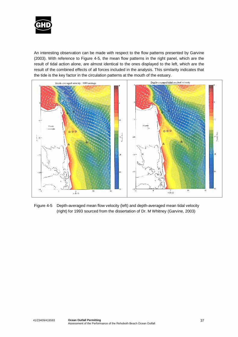
3741/23409/419593 Ocean Outfall PermittingAssessment of the Performance of the Rehoboth Beach Ocean Outfall
An interesting observation can be made with respect to the flow patterns presented by Garvine(2003). With reference to Figure 4-5, the mean flow patterns in the right panel, which are theresult of tidal action alone, are almost identical to the ones displayed to the left, which are theresult of the combined effects of all forces included in the analysis. This similarity indicates thatthe tide is the key factor in the circulation patterns at the mouth of the estuary.
Figure 4-5 Depth-averaged mean flow velocity (left) and depth-averaged mean tidal velocity(right) for 1993 sourced from the dissertation of Dr. M Whitney (Garvine, 2003)
38 41/23409/419593Ocean Outfall PermittingAssessment of the Performance of the Rehoboth Beach Ocean Outfall
4.10 ConclusionsThe following conclusions are made with respect to the model:
The current model is well calibrated and accounts for the primary physical forces governingthe flow field in the study area as indicated by the similarity of the results obtained from thecalibration and validation processes;
In terms of tidal elevation alone, the quality of the obtained solution at the outfall site (asexpressed by the level of agreement between tidal predictions and tide-only simulations) isgood. Accordingly, tidally-induced mixing processes are expected to be adequatelyrepresented in plume dispersion solutions;
Differences between modelled and measured water levels and current magnitudes observedduring the calibration and validation of the model are attributed to:
– The lack of representation in the model of currents operating at low sub-tidal frequencies(low frequency motions);
– Variations in density produced by the Delaware River discharge, that is, while the dailyvarying river discharge is included in the model, the associated density fluctuations due tosalinity and temperature are not. This comment is particularly relevant considering theadoption of a two-dimensional, depth-averaged modeling frame for the base analysis;
The model represents the wave climate in the study area fairly well;
Long-term transport trends as represented by simulated depth-averaged mean flows are ingood qualitative and quantitative agreement with previously published work. The latterfinding applies consistently throughout the entire coastal area hosting the proposed outfall;
A 2-D modelling framework is adequate for the project; and
The statistical agreement between measurements and model results is encouraging implyingthat a high level of consistency between near- and far-field analytical results is achievable.
3941/23409/419593 Ocean Outfall PermittingAssessment of the Performance of the Rehoboth Beach Ocean Outfall
5. Far Field Model Results
This chapter presents and discusses the results obtained from the calibrated model described inthe previous 4. Two scenarios associated with the operation of the proposed northern andsouthern outfalls under normal conditions have being assessed over a period of 11 months intwo-dimensional mode.
5.1 Scenario DefinitionThe two long-term far-field scenarios have been investigated with the following commoncharacteristics:
The proposed discharge of 3.4 MGD (equivalent to 0.1489 m3/s) was introduced in onemodel cell (the approximate length of the diffuser is 37 m) and the discharged effluenttreated as a hypothetical conservative, non-decaying substance with a concentration of 1kg/m3;
The discharge was modelled without interruption for a period of 11 months starting onFebruary 1st, 2010 using flow predictions for the same period provided by the model whichwas started a month earlier (January 1st 2010) to overcome any potential influence of modelwarm-up effects in the dispersion analysis of the discharged effluent; and
The hydrodynamic model was operated in two-dimensional mode and driven by tide, time-varying freshwater inflow, winds and waves as described in sections 4.5 and 4.6 of thisreport. The time step for the simulation was 1 second.
Further details of the two scenarios are:
Southern outfall (38° 43' 19.953" N, 75° 3' 37.854" W) scenario: the discharge was allocatedto a mesh cell with an area of 9,150 m2 (equivalent to a square cell with less than 100 mlength) and approximate depth of 10.8 m; and
Northern outfall (38° 43' 47.220" N, 75° 3' 30.294" W) scenario: the discharge was allocatedto a mesh cell with an area of 12,000 m2 area (equivalent to a square cell with 110 m length)and approximate depth of 12 m;
5.2 Modeling AssumptionsThe following assumptions apply to the far-field modeling exercise:
Well-mixed conditions in the Delaware estuary justify the adoption of a two-dimensional,depth-averaged frame of analysis for the project. In other words, a two-dimensional, depth-averaged frame of analysis captures reasonably well the physics of the modelledenvironment as expressed in terms of tidal elevations, circulation patterns and densityvariation.
Discharged effluent does not decay; it is only subject to dispersion and dilution by ambientcurrents. This assumption is conservative.
The effluent is assumed to mix instantaneously in the water of the receiving cell.
The background concentration of effluent in the receiving waters is nil.
40 41/23409/419593Ocean Outfall PermittingAssessment of the Performance of the Rehoboth Beach Ocean Outfall
5.3 QualificationsAnalysis has been undertaken subject to the following qualifications:
Complex biological or physical processes (such as uptake of nutrients or absorption toparticles), which can reduce the concentration of the various constituents of the effluent inthe water column, have not been modelled. This adds conservatism to the adopted modelingapproach as concentrations will remain higher if not allowed to decay.
Buoyancy effects are not represented in the far-field simulations. However, these are takeninto consideration in the near-field analysis presented in the next chapter.
5.4 Simulation Results
5.4.1 Presentation
The results from the analysis are presented in the form of:
Snapshots or instantaneous plume footprints generated at 5 day intervals to illustrate thedynamics of the plume and the correlation that exist between plume shape and wind effects(Figures D-1 to D-2, Appendix D);
Percentile maps of dilution generated using effluent concentration results extracted at 1-hourinterval for a period of two and a half months.
Note that in the assessment of percentiles of concentration, the choice of the assessmentwindow can play an important role in determining the quality of the overall results. The main roleof the window is to eliminate from consideration the effects of the initial conditions and warm-upstages of the modeling exercise, thus setting the focus of the analysis on developed conditionsalone. In the current analysis, the assessment window has been set to coincide with the last 2.5months of the hydrodynamic analysis, that is, plume behaviour is assessed after an initial periodof 6.5 months of outfall operation.
One dilution map has been generated for each scenario. The 95th percentile of effluentconcentration has been used to generate the maps.
5.4.2 Key Simulation Timeframes
The key simulation timeframes adopted in the analysis are summarised in Table 6.
Table 6 Adopted Timeframes in the Analysis (months)
Hydrodynamic (tide + freshwaterinflow + wind + waves) Simulation
Effluent Discharge 95th Percentile AssessmentWindow
12 11 2.5
4141/23409/419593 Ocean Outfall PermittingAssessment of the Performance of the Rehoboth Beach Ocean Outfall
5.4.3 Southern Outfall – Instantaneous Plume Footprints
It is noted that very low concentrations of the effluent are plotted to illustrate the trajectory of theplume and the ultimate fate of the effluent rather than to indicate the potential for impacts. Also,the concentrations are associated with a hypothetical discharge concentration in the pipe of1 kg/m3 (1000 mg/L) rather than any specific water quality parameter. As such, theinstantaneous footprints shown could be interpreted as snapshots taken with a very sensitivecamera (high detection rate) at regular time intervals during a long-duration dye tracingexperiment.
Figures D-1 and D-2 of Appendix D capture a sequence of relatively stable states of the plumereaching to the north and south of the proposed outfall.
5.4.4 Southern Outfall – Dilution Map
The dilution map shown in Figure 5-1 is an indirect depiction (based on dilution contours ratherthan concentration contours) of the potential long term footprint of the plume. The shape of theplume, in this case delimited by the 10,000:1 dilution contour, is elongated with its major axisrunning parallel to the coast. There is no evidence of plume encroachment on the coast of anyform which indicates that there are no risks for primary contact recreation activities. The use ofthe 10,000:1 dilution contour to delimit the plume footprint yields a rather conservativerepresentation of the latter. From a regulatory viewpoint, it could be argued that the 200:1 or500:1 dilution contours (both enclosing areas that are significantly smaller than the areadelimited by the 10,000:1 dilution contour) would be adequate and should be used for thispurpose. Such contours, however, do not appear in the current far-field analysis owing to thecombined effects of low discharge volume and the resolution of the far-field model in the outfallarea.
Total areas enclosed within the dilution contours are listed in Table 7. As seen from the table,the predicted area enclosed by the 5000:1 dilution contour is as low as 1 ha.
Table 7 Southern Outfall - Total Area within a Given Dilution Contour
Dilution Contour 95% probability area (ha)
10000 6
5000 1
42 41/23409/419593Ocean Outfall PermittingAssessment of the Performance of the Rehoboth Beach Ocean Outfall
5.4.5 Northern Outfall
For the Northern outfall and with reference to Figure 5-2, the shape and extent of the predictedplume generated at the (potential) northern outfall is similar to the one predicted at the(potential) southern outfall leading to identical findings; that is, there is no evidence of plumeencroachment on the coast which indicates that there are no risks for primary contact recreationactivities.
Total areas enclosed within the dilution contours are listed in Table 8. As seen from the table,the area enclosed by the 5000:1 dilution contour is less than 1 ha.
Table 8 Northern Outfall - Total Area within a Given Dilution Contour
Dilution Contour 95% probability area (ha)
10000 <5
5000 <1

4341/23409/419593 Ocean Outfall PermittingAssessment of the Performance of the Rehoboth Beach Ocean Outfall
Figure 5-1 Southern Outfall: Contour plot showing the 95th percentile of dilution after 11 monthof outfall operation
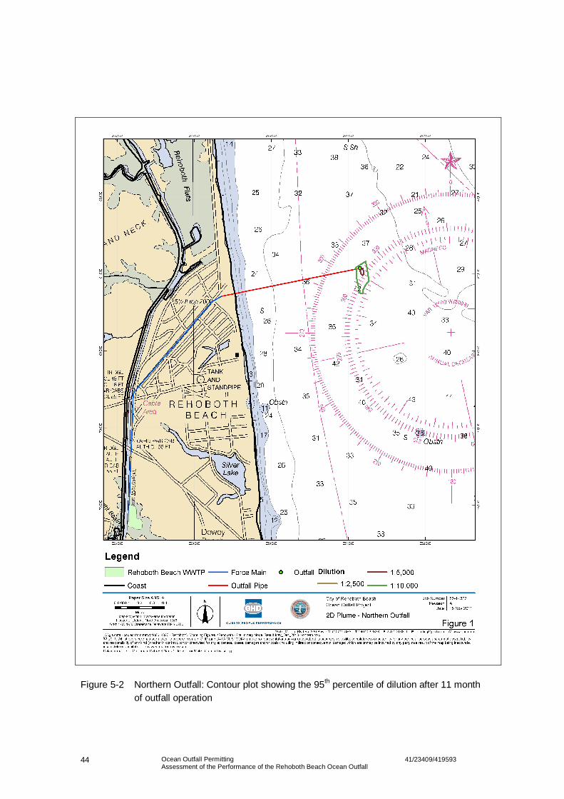
44 41/23409/419593Ocean Outfall PermittingAssessment of the Performance of the Rehoboth Beach Ocean Outfall
Figure 5-2 Northern Outfall: Contour plot showing the 95th percentile of dilution after 11 monthof outfall operation
4541/23409/419593 Ocean Outfall PermittingAssessment of the Performance of the Rehoboth Beach Ocean Outfall
5.5 ConclusionsBased on the far-field analysis of effluent plume advection and dispersion for both potentialoutfall locations (north and south) and subject to (1) the discharge characteristics specified insection 5.1, (2) the adopted 2-D modelling frame, (3) year 2010 meteorological conditions andqualifications presented in section 5.3, it is observed that both plume footprints as identified bythe 10,000:1 dilution contour:
Form offshore and remain in the vicinity of their respective sources;
Assume somewhat elongated shapes with a major axis running parallel to the coast;
Are subject to the variation in magnitude of the combined effects of the driving forces (tide,winds, waves and freshwater inflows); and
Are not predicted to reach the coast.
For the 11-month simulation period starting February 1, 2010, the maximum predicted (at 1 hourinterval) effluent concentration for the proposed southern outfall did not exceed 0.3 mg/L (Notethe concentration is the result of the discharge of effluent at a hypothetical concentration of1000 mg/L in the pipe). This is equivalent to a minimum dilution in excess of 3000:1. Owing tothe identified similarities in receiving water conditions and statistical plume footprints at bothpotential outfall sites, it is expected that the maximum predicted (instantaneous) effluentconcentration at the proposed northern outfall will be of similar magnitude. Because of thesimilarity of the results, the choice of outfall site can be based on factors other thanhydrodynamics and dilution.

46 41/23409/419593Ocean Outfall PermittingAssessment of the Performance of the Rehoboth Beach Ocean Outfall
6. Near Field Modeling
6.1 IntroductionNear-field modeling of the proposed ocean outfall has been undertaken using CORMIX, thesoftware preferred by the USEPA and state regulators. The diffuser configuration previouslyproposed comprised a Y shape in plan with symmetrical arms, each with 8 vertical risers, asdescribed in Lawler, Matusky & Skelly Engineers (2003) and Stearns & Wheler (2005). Eachriser terminated with two nozzles.
However, this Y type configuration (presented in Appendix A of the modeling report) cannot beimplemented in CORMIX directly, and hence a projected linear diffuser with a rosettearrangement was adopted (consistent with previous modeling). The linear diffuser with rosetteconsisting of four ports per riser is shown in Figure 6-1. Details of the diffuser configuration arepresented in Table 9.
Figure 6-1 Schematic Diagram of Modeled Diffuser
Port
Riser

4741/23409/419593 Ocean Outfall PermittingAssessment of the Performance of the Rehoboth Beach Ocean Outfall
Table 9 Diffuser Configuration as Initially Modeled
Parameter Value
Diffuser length 120 ft (37 m)
Distance from shore 6,000 ft (1823 m)
Port height from seabed 1.5 ft (0.5 m)
Port diameter 3 inches (0.075 m)
Number of risers 8
Number of ports per riser 4
Total number of openings (ports) 32
Alignment of ports Horizontal
The CORMIX software has been used on the basis of its preferred status (by USEPA and stateregulators). CORMIX offers the following advantages in conducting near-field modeling:
Multiple ports in the form of complex linear diffusers (such as rosettes) can be implementedusing the pre-processing tools within CORMIX. The simulation of multi-port diffusers allowsthe model to assess plume merging and interaction with the ocean floor. It should be notedthat for this reason, it is difficult to compare model outcomes with other near-field modelswhich may typically reflect higher dilutions; and
CORMIX allows three types of vertical density specifications; (a) linear, (b) two layer systemwith constant densities and density jump, and (c) constant density surface layer with lineardensity profile in the bottom layer separated by a density jump. For the present scenarios,the second option has been assessed as this presents the most conservative verticalstratification scenario;
6.2 AimsThe preliminary diffuser design was based on “…generally accepted principles…” aimed toprovide a balance between dilution and costs (Lawler, Matusky & Skelly Engineers 2003). Thefirst aim of the current near-field modeling exercise is therefore to verify that the dilutions andmixing patterns described in previous modeling reports can be replicated. A second, moregeneral aim, becomes possible through the availability of additional and better quality receivingwater data; that is, to test the performance of the diffuser for the expected spectrum of ambientconditions.
6.3 Target DilutionA key outcome of near-field modeling is to confirm whether sufficient dilution will be achieved inorder to meet environmental protection criteria. The definition of what the target dilution shouldbe therefore becomes an important criterion, with the typical process being to comparedischarge concentrations (of pollutants of concern) with nominated receiving water standards.
48 41/23409/419593Ocean Outfall PermittingAssessment of the Performance of the Rehoboth Beach Ocean Outfall
In the absence of specific values, a target dilution factor of 100 would generally be chosen,though it may be that a lower value (e.g. 50) will meet all environmental protectionrequirements.
For TSS, the discharge of 5.4 mg/L is already lower than the water quality limits.
6.4 Discharge CharacteristicsThe discharge characteristics utilized in the model are presented in Table 10.
Table 10 Rehoboth Beach WWTP Current Effluent Performance Data
Parameter Measured Concentration
BOD 2.8 mg/L
TSS 5.4 mg/L
TN 6.2 mg/L
TP 0.3 mg/L
Ammonia 0.769 mg/L
Temperature 64.6 °F (18.1 °C)
Enterococcus 2.7 Colonies / 100 mL
Notes:
1. Performance data based on January 2007 – July 2010. Annual average flow for reported period was1.1 mgd.
6.5 Input DataThe availability of data was addressed in Chapter 3. Of most relevance to the near-fieldmodeling exercise are field measurements of ambient conditions, comprising salinity,temperature, and the direction and magnitude of currents.
Figure 6-2 provides a summary of the relative occurrence of each of the primary bands ofcurrent magnitude. The figure shows that near-zero or very low currents occur for some 13% ofthe monitoring period, with the median current falling within the 1.0 – 1.3 ft/s (0.3 to 0.4 m/s)band. The maximum current band (> 2.0 ft/s or 0.6m/s) occurred for only 3% of the record.
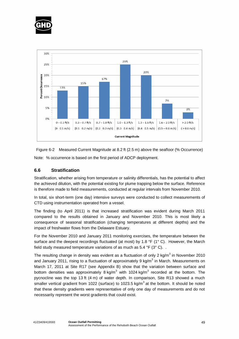
4941/23409/419593 Ocean Outfall PermittingAssessment of the Performance of the Rehoboth Beach Ocean Outfall
Figure 6-2 Measured Current Magnitude at 8.2 ft (2.5 m) above the seafloor (% Occurrence)
Note: % occurrence is based on the first period of ADCP deployment.
6.6 StratificationStratification, whether arising from temperature or salinity differentials, has the potential to affectthe achieved dilution, with the potential existing for plume trapping below the surface. Referenceis therefore made to field measurements, conducted at regular intervals from November 2010.
In total, six short-term (one day) intensive surveys were conducted to collect measurements ofCTD using instrumentation operated from a vessel.
The finding (to April 2011) is that increased stratification was evident during March 2011compared to the results obtained in January and November 2010. This is most likely aconsequence of seasonal stratification (changing temperatures at different depths) and theimpact of freshwater flows from the Delaware Estuary.
For the November 2010 and January 2011 monitoring exercises, the temperature between thesurface and the deepest recordings fluctuated (at most) by 1.8 °F (1° C). However, the Marchfield study measured temperature variations of as much as 5.4 °F (3° C). .
The resulting change in density was evident as a fluctuation of only 2 kg/m3 in November 2010and January 2011, rising to a fluctuation of approximately 9 kg/m3 in March. Measurements onMarch 17, 2011 at Site R17 (see Appendix B) show that the variation between surface andbottom densities was approximately 8 kg/m3 with 1024 kg/m3 recorded at the bottom. Thepycnocline was the top 13 ft (4 m) of water depth. In comparison, Site R13 showed a muchsmaller vertical gradient from 1022 (surface) to 1023.5 kg/m3 at the bottom. It should be notedthat these density gradients were representative of only one day of measurements and do notnecessarily represent the worst gradients that could exist.
50 41/23409/419593Ocean Outfall PermittingAssessment of the Performance of the Rehoboth Beach Ocean Outfall
Offshore, beyond the 30 feet depth contour, density differentials in the 1 to 3 kg/m3 range areexpected to be common during the spring and autumn period with peaks reaching in the 6 to9 kg/m3 range during high river inflow periods that could last for up to two weeks and occur 3-4times during the same season. These peak ranges (of estimated density differential) aresubstantially narrower in shallow coastal waters (where the proposed outfall is located) and,based on the collected evidence to date, could reach up to 3-4 kg/m3.
Temperature and density data have been utilized in near-field modeling, in order to test theimpact on dilution for differing strengths of stratification.
6.7 Model Scenario DefinitionA total of nine different cases have been modeled. The first of these is a base case, as definedby the previously proposed diffuser configuration, a near zero ambient flow, and nostratification. The base case scenario is consistent with previous findings (Lawler, Matusky &Skelly Engineers 2003) as these had been tested for diffuser performance as well as costs.However, the diffuser design needs to be further tested for newly acquired (i.e. most current)ambient conditions data, and for the influence of stratification. These tests have beencompleted in Cases 001 to 009, as described below.
The following describes the nine cases that were investigated:
Case 000 represents the base condition consistent with the preliminary design (modeled asa linear diffuser) albeit with very low ambient currents around 0.13 ft/s (0.04 m/s). Theprimary reason for the choice of low ambient current was that it sets the worst mixingperformance under a non-stratified receiving environment (In this model setup, CORMIXdoes not allow specification of currents less than 0.13 ft/s (0.04 m/s) as this creates plumeinstabilities). This ambient current typically corresponds to a nontidal velocity; however,ADCP measurements in the vicinity of the proposed outfall indicate that velocities between 0and 0.3 ft/s (0 and 0.1 m/s) occur for more than 13% of the time. Hence the dilutions(possibly worst case) arising from this scenario are likely to have a low probability ofincidence. It has also been observed from the CTD data that whenever vertical stratificationdoes not exist, the water column density is typically 1024 kg/m3.
Cases 001 to 003 investigate the influence of increasing ambient current. The basis ofselection of currents can be seen with reference to Figure 6-2. Case 003 represents themost frequently occurring current condition, and is therefore of value when considering themedian condition at the study site. A case corresponding to the high ambient currentcondition around 2 ft/s (0.6 m/s) is not presented, as this simply confirms that significantdilution will occur when ambient currents are strong.
Case 004 investigates the impacts on dilutions when moderate stratification is evident in thereceiving environment, with a differential of 1.5 kg/m3. The latter value is typically associatedwith low to average inflow periods (e.g. Delaware River discharges in the 10,600 to 18,000cfs (300 to 500 m3/s) range) and has a relatively high probability of occurrence at offshorelocations during the spring and autumn seasons. Near the coast however, the value isexpected to be encountered and exceeded only during periods of high river inflows lastingfor up to two weeks and occurring more than once during the same season.
5141/23409/419593 Ocean Outfall PermittingAssessment of the Performance of the Rehoboth Beach Ocean Outfall
Case 005 involves the consideration of a longer diffuser with twice the length of the basecase scenario while halving the number of ports per riser from four to two. While longer, thistype of diffuser system can be easier to construct and maintain since there are a reducednumber of external connections per riser. A cost analysis has not been undertaken todetermine if this diffuser arrangement is less expensive than the preliminary design.
Case 006 tests the effect of mixing using a theoretical wind speed of 16.4 ft/s (5 m/s). It isnoted that a higher wind speed could have been selected, but that high periods of wind areoften directly linked to larger waves, with the combination of the two forces leading togreater mixing. Given the purpose of the nearfield assessment is to consider potentialimpacts, it is appropriate to select a moderate wind.
Case 007 investigates the effect of increasing vertical density stratification for the mediancurrent condition. CTD data for the region indicates the presence of seasonal densitystratification within the water column and the largest difference observed was eight (8)kg/m3 between surface (1016 kg/m3) and bottom (1024 kg/m3). A linear gradient in densityhas been prescribed in CORMIX. This case is simulates the poorer mixing conditionsassociated with a stratified environment at the proposed outfall site.
Case 008 assesses the combination of large ambient currents around 2 ft/s (0.6 m/s) withthe same degree of stratification described in Case 007.
6.8 Modeling ResultsThe results of CORMIX modeling are presented in this section.
As previously described, the base case (Case 000) reflects the previously proposed diffuserconfiguration and typical ambient conditions (without consideration of current magnitudes). Allother cases investigate variations in ambient and diffuser parameters.
Dilutions from all nine simulations have been plotted in Figure 6-3 (Cases 000 – 006) andFigure 6-4 (Cases 007 – 008). Results are also summarized in Table 11.
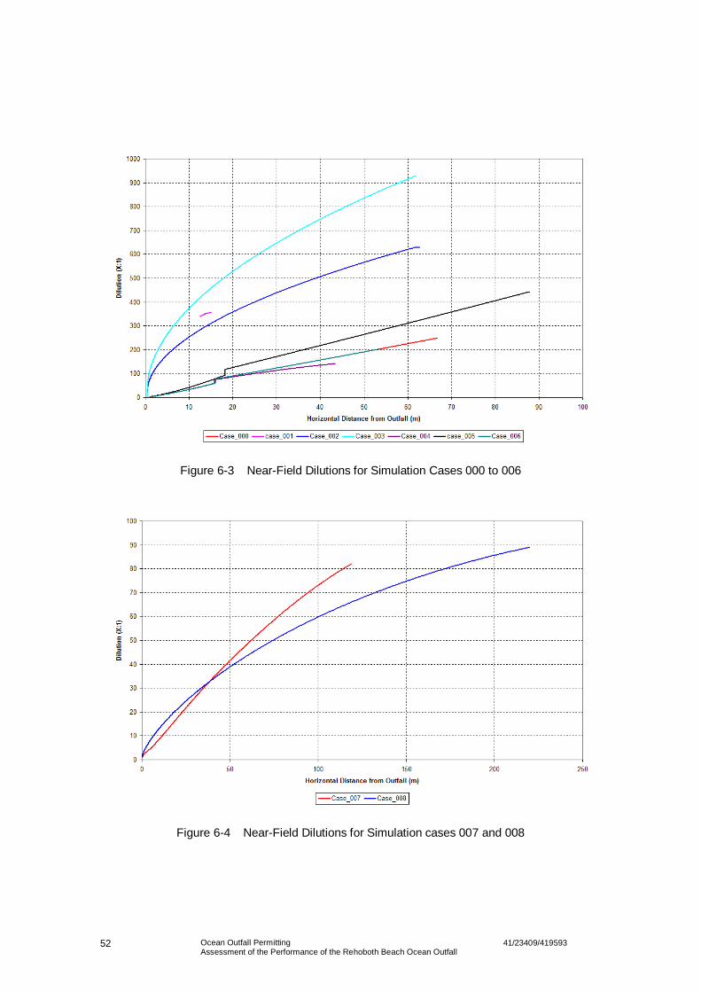
52 41/23409/419593Ocean Outfall PermittingAssessment of the Performance of the Rehoboth Beach Ocean Outfall
Figure 6-3 Near-Field Dilutions for Simulation Cases 000 to 006
Figure 6-4 Near-Field Dilutions for Simulation cases 007 and 008
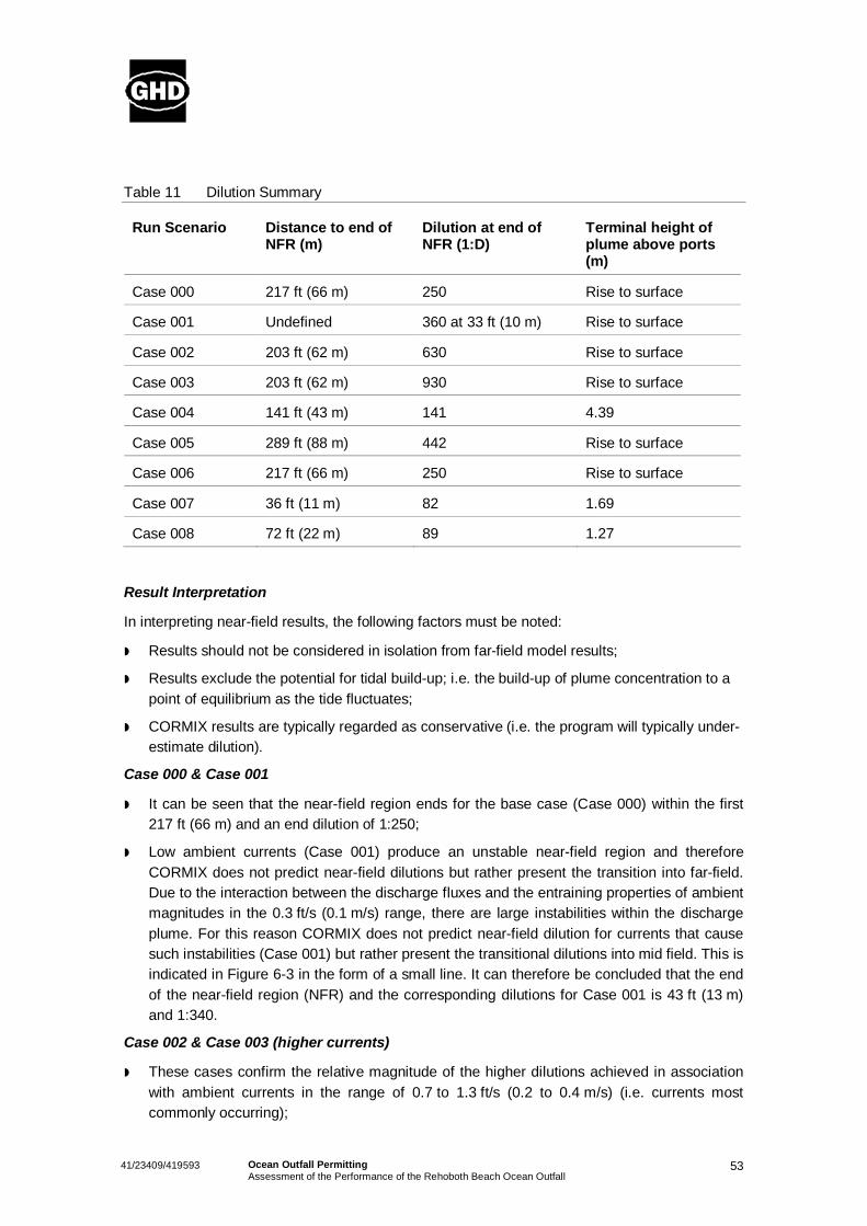
5341/23409/419593 Ocean Outfall PermittingAssessment of the Performance of the Rehoboth Beach Ocean Outfall
Table 11 Dilution Summary
Run Scenario Distance to end ofNFR (m)
Dilution at end ofNFR (1:D)
Terminal height ofplume above ports(m)
Case 000 217 ft (66 m) 250 Rise to surface
Case 001 Undefined 360 at 33 ft (10 m) Rise to surface
Case 002 203 ft (62 m) 630 Rise to surface
Case 003 203 ft (62 m) 930 Rise to surface
Case 004 141 ft (43 m) 141 4.39
Case 005 289 ft (88 m) 442 Rise to surface
Case 006 217 ft (66 m) 250 Rise to surface
Case 007 36 ft (11 m) 82 1.69
Case 008 72 ft (22 m) 89 1.27
Result Interpretation
In interpreting near-field results, the following factors must be noted:
Results should not be considered in isolation from far-field model results;
Results exclude the potential for tidal build-up; i.e. the build-up of plume concentration to apoint of equilibrium as the tide fluctuates;
CORMIX results are typically regarded as conservative (i.e. the program will typically under-estimate dilution).
Case 000 & Case 001
It can be seen that the near-field region ends for the base case (Case 000) within the first217 ft (66 m) and an end dilution of 1:250;
Low ambient currents (Case 001) produce an unstable near-field region and thereforeCORMIX does not predict near-field dilutions but rather present the transition into far-field.Due to the interaction between the discharge fluxes and the entraining properties of ambientmagnitudes in the 0.3 ft/s (0.1 m/s) range, there are large instabilities within the dischargeplume. For this reason CORMIX does not predict near-field dilution for currents that causesuch instabilities (Case 001) but rather present the transitional dilutions into mid field. This isindicated in Figure 6-3 in the form of a small line. It can therefore be concluded that the endof the near-field region (NFR) and the corresponding dilutions for Case 001 is 43 ft (13 m)and 1:340.
Case 002 & Case 003 (higher currents)
These cases confirm the relative magnitude of the higher dilutions achieved in associationwith ambient currents in the range of 0.7 to 1.3 ft/s (0.2 to 0.4 m/s) (i.e. currents mostcommonly occurring);
54 41/23409/419593Ocean Outfall PermittingAssessment of the Performance of the Rehoboth Beach Ocean Outfall
Case 002 has a NFR of 203 ft (62 m) and end point dilution of 1:630 while Case 003 has aNFR of 203 ft (62 m) but appreciably higher dilution of 1:930.
Case 005 (Longer Diffuser)
Case 005 confirms the benefit to dilution in doubling the length of the diffuser and therebyreducing the total number of ports per riser. The NFR is 289 ft (88 m) with dilution of 1:442.It should be noted that the longer diffuser may be more cost effective than the originallyproposed Y-diffuser as it is a simpler construction, while possessing a similar length to thecumulative lengths of the Y-diffuser.
Case 006 (influence of wind)
Surface winds do not impact dilutions in the near-field as demonstrated by Case 006.Results are identical to Case 000;
Cases 004, 007, 008 (Stratification)
Cases (004, 007 and 008) show a decrease in dilution. This demonstrates that vertical(stable) density stratification inhibits mixing of the discharge plume under the simulatedconditions. The plumes from all the three scenarios are vertically trapped at 14.4, 5.5, and4.2 ft (4.39, 1.69 and 1.27 m) from the seafloor; and
With large vertical stratification, the dilutions potentially decrease to less than 1:90,irrespective of whether ambient currents are large or small. This scenario therefore imposesthe most significant mixing and dilution constraint.
Flow Direction
All currents modeled were taken to flow perpendicular to the diffuser line (or parallel to thecoast) as the ADCP data indicates that this was the direction of prevailing currents.
There are brief instances (i.e. of low incidence) where currents flow perpendicular to the shore,though these will almost always be for short durations only, and dilution in the near-field will stilloccur.
The results of the far field model were utilized to confirm that the overall dilutions from thisarrangement will not vary compared to the dilution seen when currents flow perpendicular to thediffuser arrangement.

5541/23409/419593 Ocean Outfall PermittingAssessment of the Performance of the Rehoboth Beach Ocean Outfall
6.9 ConclusionsNear-field dilution performance has been simulated based on a linear diffuser. Nine simulationsin total were conducted, with Case 000 reflecting the projected rosette design of the previouslyproposed Y type diffuser (i.e. base case). The projected preliminary design is essentially alinear diffuser. The modeled cases investigated the effect of ambient current speed, ambientvertical density stratification and also the effect on dilution by increasing the length of thediffuser. The following conclusions can be derived from this study:
Overall, a high level of dilution should be achieved.
The linear diffuser achieved a dilution in excess of 1:250 for an un stratified ocean withclose to zero ambient current magnitudes. As typically expected, dilutions increased withincreasing current magnitudes and the most frequent current of 0.3 m/s results in dilution of1:930 within 203 ft (62 m) of the discharge;
Vertical density stratification provides some limitation to mixing, though this appears unlikelyto lead to any impact of consequence. It is indicated that the diffuser should be optimized forworst case ambient stratification. Recognizing the conservatism of CORMIX, a dilution ofonly 1:82 is achieved at a distance of 390 ft (119 m) when the ambient current speed isclose to zero and an ambient density difference of 8 kg/m3 between surface and bottomwater column is included. The mixing outcome does not change significantly with increasingcurrents;
There is potential merit in doubling the length of the diffuser (Case 005) while reducing thenumber of ports per riser to two as this diffuser offers better dilution compared to thepreliminary design. The longer diffuser can potentially help overcome the mixing constraintswhen the water column is density stratified. A linear diffuser system can also enable betterhead loss and port exit velocity control, in comparison to a Y-shaped design. This diffusermay also be simpler to construct (one single trench) and maintain (simpler risers and ports).
6.10 QualificationsConclusions relate to the modeled cases only. Model input data have been sourced fromvarious reports and measured data as indicated.
All the modeled cases can be interpreted to be linear diffusers, lying perpendicular to theprevailing currents (north-south).
56 41/23409/419593Ocean Outfall PermittingAssessment of the Performance of the Rehoboth Beach Ocean Outfall
7. Conclusions and Recommendations
7.1 Far Field/Plume DispersionConclusions are offered on the basis of the far-field analysis of effluent plume advection anddispersion for both potential outfall locations (north and south). These are subject to (1) thedischarge characteristics specified in section 5.1, (2) the adopted 2-D modelling frame, (3) year2010 meteorological conditions and qualifications presented in section 5.3. It is observed thatfor both the north and south location, plume footprints as identified by the 10,000:1 dilutioncontour:
Form offshore and remain in the vicinity of their respective sources;
Assume somewhat elongated shapes with a major axis running parallel to the coast;
Are subject to the variation in magnitude of the combined effects of the driving forces (tide,winds, waves and freshwater inflows); and
Are not predicted to reach the coast.
For both proposed outfall sites, total areas enclosed within the 5000:1 dilution contour are aslow as 1 ha.
For the 11-month simulation period starting February 1, 2010, the minimum predicted (at 1 hourinterval) effluent dilution for the proposed southern outfall was greater than 3000:1. Owing to theidentified similarities in receiving water conditions and statistical plume footprints at bothpotential outfall sites, it is expected that the minimum predicted effluent dilution at the proposednorthern outfall will be of similar magnitude. Because of the similarity of the results, the choiceof outfall site can be based on factors other than hydrodynamics and dilution.
7.2 Near Field/DiffusersNear-field dilution performance has been simulated based on a linear diffuser. Nine simulationsin total were conducted, with Case 000 reflecting the projected rosette design of the previouslyproposed Y type diffuser (i.e. base case). The projected preliminary design is essentially alinear diffuser. The modeled cases investigated the effect of ambient current speed, ambientvertical density stratification and also the effect on dilution by increasing the length of thediffuser. The following conclusions can be derived from this study:
Overall, a high level of dilution should be achieved;
The linear diffuser achieved a dilution in excess of 1:250 for an unstratified ocean with closeto zero ambient current magnitudes. As typically expected, dilutions increased withincreasing current magnitudes and the most frequent current of 0.3 m/s results in dilution of1:930 within 203 ft (62 m) of the discharge;
Vertical density stratification provides some limitation to mixing, though this appears unlikelyto lead to any impact of consequence. It is indicated that the diffuser should be optimized forworst case ambient stratification. Recognizing the conservatism of CORMIX, a dilution ofonly 1:82 is achieved at a distance of 390 ft (119 m) when the ambient current speed isclose to zero and an ambient density difference of 8 kg/m3 between surface and bottom

5741/23409/419593 Ocean Outfall PermittingAssessment of the Performance of the Rehoboth Beach Ocean Outfall
water column is included. The mixing outcome does not change significantly with increasingcurrents;
There is potential merit in doubling the length of the diffuser (Case 005) while reducing thenumber of ports per riser to two as this diffuser offers better dilution compared to thepreliminary design. The longer diffuser can potentially help overcome the mixing constraintswhen the water column is density stratified. A linear diffuser system can also enable betterhead loss and port exit velocity control, in comparison to a Y-shaped design. This diffusermay also be simpler to construct (one single trench) and maintain (simpler risers and ports).
58 41/23409/419593Ocean Outfall PermittingAssessment of the Performance of the Rehoboth Beach Ocean Outfall
8. References
C. Reid Nichols and Robert G. Williams, 2009, Encyclopedia of Marine Science, Library ofCongress
Fischer, H.B., E.J. List, R.C.Y. Koh, J. Imberger, and N.H. Brooks, Mixing in Inland and CoastalWaters, Academic Press, New York, 1979.
GARVINE, R.W., Letter to Stearns and Wheler, 2003
Good Modeling Practice Handbook, STOWA/RIZA 1999, Dutch Department of Public Works,Institute for Inland Water Management and Waste Water Treatment, Report 99.036
Lawler, Matusky & Skelly Engineers, 2003. Regional Effluent Disposal Study for the City ofRehoboth Beach, Delaware – Supplemental Dilution Modeling.
Sharp, J., Ed., 1984: The Delaware Estuary: Research as background for estuarinemanagement and development. Delaware River and Bay Authority Rep. DEL-SG-03-84,University of Delaware Sea Grant College Program, Lewes, Delaware, 340 pp.
USEPA (U.S. Environmental Protection Agency) Technical Support Manual: Waterbody Surveysand Assessment for Conducting Use Attainability Analyses, Volume II, Estuarine Systems,Technical Report, Office of Water Regulations and Standards, USEPA, Washington, DC,1984a.
Whitney, M.M, 2003: Simulating the Delaware Coastal Current. Ph.D. dissertation, University ofDelaware, 284 pp.


41/23409/419593 Ocean Outfall PermittingAssessment of the Performance of the Rehoboth Beach Ocean Outfall
GHD
201 Charlotte Street Brisbane QLD 4000GPO Box 668 Brisbane QLD 4001T: (07) 3316 3000 F: (07) 3316 3333 E: [email protected]
© GHD 2011
This document is and shall remain the property of GHD. The document may only be used for the purposefor which it was commissioned and in accordance with the Terms of Engagement for the commission.Unauthorised use of this document in any form whatsoever is prohibited.
Document Status
RevNo. Author
Reviewer Approved for Issue
Name Signature Name Signature Date
Ivan Botev Ross Fryar
Alexis Berthot