cis 100 databases in excel creating, sorting, …staff notes for...c:\users\dcraig\desktop\lecture...

$: CIS 100 Databases in Excel Creating, Sorting, …staff notes for...C:\Users\dcraig\Desktop\lecture notes for chapter 6 databases revised fall 2016-student version.docx Page 7 of 18$
C:\Users\dcraig\Desktop\lecture notes for chapter 6 databases revised fall 2016-student version.docx Page 1 of 18

CIS 100 Databases in Excel

Creating, Sorting, Querying a Table and Nesting Functions

Objectives

Create and manipulate a table

Deleting duplicate records

Delete sheets in a workbook

Add calculated columns to a table

Use icon sets with conditional formatting

Use the VLOOKUP function to look up a value in a table

Print a table

Add and delete records and change field values in a table

Sort a table on one field or multiple fields

Query a table

Apply database Functions SUMIF and COUNTIF

Display automatic subtotals

Use Group and Outline features to hide an unhide data

Creating the Database (also called a Table)

In A5, type Sales Reps Database

Press enter

Select from A5 to H5

Right click in the selected cells

Click Format Cells

Click the alignment tab

In the text alignment area, click the horizontal ▼

Click center across selection

Click OK

With the cells still selected, on the home tab, in the styles group, click the cell styles button [more button on a wide screen monitor]

In the gallery, click on Title Entering the Field Names

Click in A6, type first in all lower case letters

Type the first five of the field names across row 6—[only type first, last, city, state, sales,—we will add three fields later]

Select the field names and center them in their cells

With the cells still selected, in the styles group, click on the cell styles button

Click on Heading 3


Because the cells are still selected, click outside of the selected cells Changing the Sheet Name and Changing the Tab Color

Double click the sheet1 tab

Type sales reps as the name

Press enter

Right click the sheet tab

Click tab color

Click one of the blues

Saving the workbook Save the file on your usb drive as sales rep records

Converting Cells to a Database (table is the current term for a database) You are going to do two things at once. You will convert the cells into a table (database) and use a predesigned format to determine how it will look.

Select the field names [only need to select field names now, not a first row also]

Make sure you are on the home ribbon tab

In the styles group, click Format as table

In the table gallery, in the medium section, click on column 2, row 1

Click in the My table has headers option so that Excel knows you have field names as the first row

Click OK

You are not stuck with every single formatting attribute that the predesigned table format contains. You can change individual attributes.

Formatting the Fields of the Database before Entering Records Because you formatted the table for using a gallery format, if you want the formatting of the cells containing records to be any different from the gallery format, you must make that format change now in the first row where records will go. Centering State Field

Select D7

Click the Home ribbon tab; in the Alignment group, click the center button


Formatting Sales Field for a Comma as Thousands Separator

Click in E7 alone

Right click E7, the sales cell on the first record row

Click format cells

Click the number tab

In the category group, click number

Click in the option for the thousands separator (a comma every 3 digits to the left of the decimal point)

You want whole numbers only, even though you are formatting amounts of money. Formatting for whole dollars—no Cents

Click the decimal places ▼ two times so that no decimal numbers show—no cents

Click OK The sales figures will now show with commas as the thousands separator and will round to the nearest dollar. Modifying the Table Style Even though you cannot modify or delete an existing style, you can duplicate an existing style and make changes to the duplicate and save it under another name. That’s what we will do here.

Click in A7

Make sure you are on the Home Ribbon tab

In the Styles group, click Format as Table button

In the medium section, right click the medium blue style in column 2, row 1 Notice that modify and delete are dimmed so that they cannot be chosen. Now we will make a duplicate of the style and then make the changes that we want to this duplicate style.

On the shortcut menu, click Duplicate

You see the Modify Table Style dialog box; the table element section lists things that can be modified. You won’t change it very much. You will change an existing style by adding bolding and then save it under another name.

Since this is going to be a new style, Click in the Name text box

Delete the existing name, and type blue_style

In the table element list, click on Whole Table to make sure it is selected You want to bold the font in the entire table.

Click Format to see the Format Cells dialog box

In the Font style area, click on Bold


Click the color ▼

In the color palette, click on the next to the bottom color in the second column.

Click OK (to close the dialog box) You have just created a new style by taking an existing style, duplicating it, making a couple of changes, and saving it under a new name. Changing the Field Names Font to White for Readability

Select the field names

Up on the ribbon, in the Font group, click the font color ▼

Click white

Click outside of the selected cells Adding Records to the Table

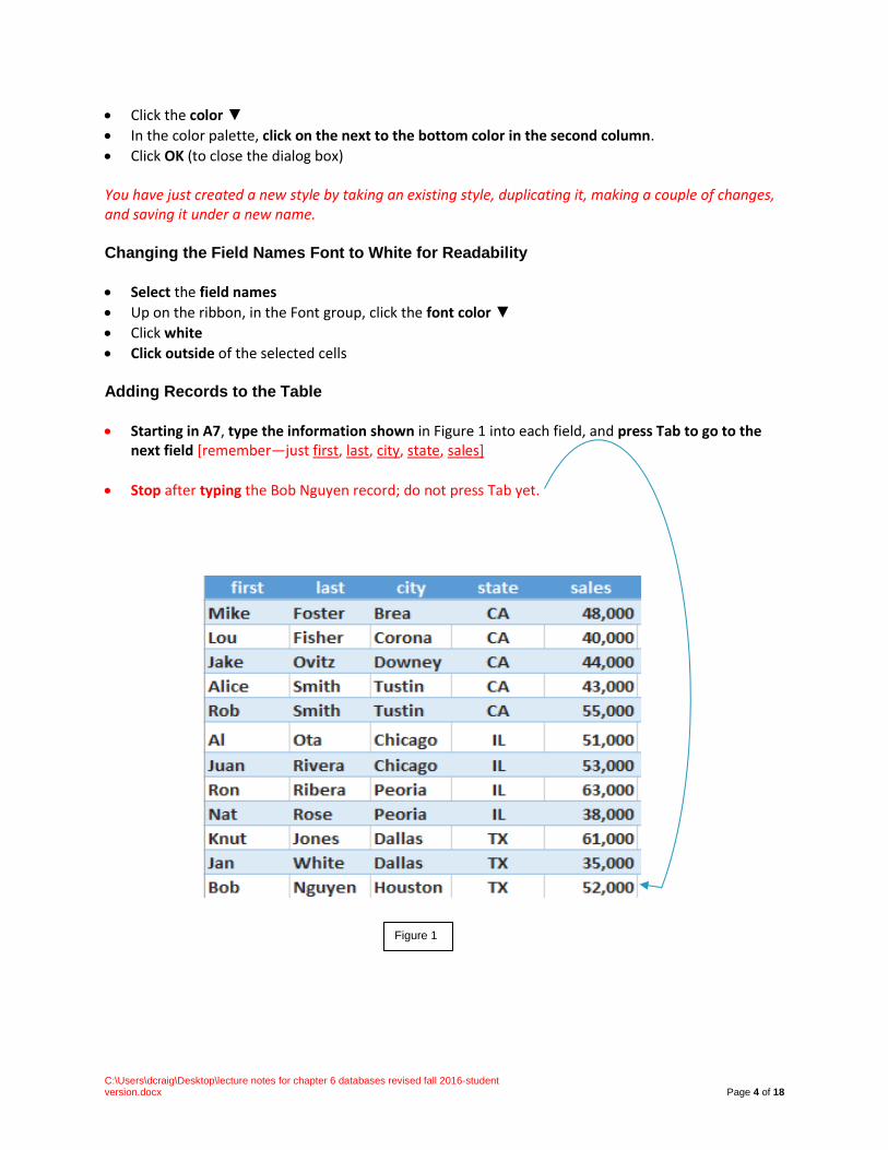
Starting in A7, type the information shown in Figure 1 into each field, and press Tab to go to the next field [remember—just first, last, city, state, sales]

Stop after typing the Bob Nguyen record; do not press Tab yet.

Figure 1


On row 19, we will deliberately type a duplicate record.

Press tab to move on to row 19 if you are not there already

Again type the information for Knut Jones.

Press enter at the end of this record to end your database

Proofread your records and make any necessary corrections. Duplicate Records and how to Get them out of your Database It is easy to end up with a duplicate record in your database if they have not been sorted yet. This is especially true if more than one person enters the records. Fortunately, there is a way to delete records without having to read through all of them.

Click anywhere in the database.

Click on the Tables Tools Design ribbon tab.

In the tools group, click the Remove Duplicates button

In the Remove Duplicates dialog box, Click the Select All button

Click OK.

Click OK again to finish up. NOTE: To add rows later, you can just click in the last cell of a completed row and press Tab.

Click outside of the selected cells Add New Fields to a table (add to the right)

Click in F6

Type gender as the field name, and press enter

Click in G6

Type comm as the field name, and press enter

Click in H6

Type comment as the field name, and press enter Validating Information being Entered into the Cells

Validation is putting a rule or rules on a cell that tells Excel what you will allow in a cell. In other words, what you allow is valid. It will prevent the user from entering incorrect (invalid) information in the cell.

Select all the cells in the gender field, but not the title

Click the Data ribbon tab

In the Data Tools group, click on data validation button

On the drop down menu, click data validation


There are three tabs in the Data Validation dialog box

Click the Allow ▼ Figure 2 shows what the choices in the Allow menu mean:

Item on list What it allows

any value Anything

whole number whole numbers in a specific range

decimal number decimal numbers

List only an item from a list

date a range of dates

Time a range of times

text length a certain length of text

custom can specify a formula—example: >25 requires entry to be more than 25 Figure 2

Click List You can do lists two ways: just type the list in the dialog box or if you have a longer list typed somewhere else in the sheet, just refer to its location. We have a very short list; therefore, we will merely type the list in the dialog box.

In the source box, type f,m

Click in the in-cell dropdown option to the right of the allow text box. You don’t want a drop down box showing f and m each time you type a record because it just gets in the way and users can remember the two choices anyway without a choice showing each time.

Click the Error Alert Tab to prepare an error message that will show if the user makes a mistake.

Make sure that the Show error alert after invalid data is entered option is checked

Click the style ▼ to see the choices (we will use the stop sign)

In the Title text box, type Gender Invalid

Click in the Error message text box

Type Gender must be entered as f or m. Please try again.

Click OK Adding Data to the New Gender Field

Click in the first blank cell in the new field—Enter the information in Figure 3.

F7 m F14 m

F8 f F15 m

F9 m F16 m

F10 f F17 f

F11 m F18 m

F12 m

F13 m

Figure 3


Select the gender cells and click the home ribbon tab

In the alignment group, click the center button Adding Data to the New Commission (Comm) Field for 5%

Make sure you are on the Data ribbon tab

Click in G7

Type = [ @ sales ] * 5% Note: Do not type the information in this note. If sales had been a field name with more than one word, you would have had to type it like this [@[sales]]*5%

Press Enter Use Conditional Formatting with Icons

Select all the cells with commissions in them

Click on the home ribbon tab

In the styles group, click Conditional formatting

Click New Rule

In the bottom half of the dialog box, click the Format Style ▼

Click the ▼ for Icon Sets in the list

Click the icon style ▼

Scroll down to and click the 5 arrows (colored) style near the bottom of the list

In the Type area at the right of the dialog box, click the top ▼

Change it to Number

Change the rest of the type boxes to number

In the Value area, on the same line as the green arrow, delete the 0 and type 2700 This means that Excel will add a green up arrow if the number is over or equal to 2700

In the second value text box, delete the 0 and type 2100 This means that Excel will add a yellow right up arrow if the number is under 2700 and more than or equal to 2100

In the Third value text box, delete the 0 and type 2000 This means that Excel will add a yellow right arrow if the number is under 2100 and more than or equal to 2000

In the fourth value text box, delete the 0 and type 1900

This means that Excel will add a yellow right down arrow if the number is under 2000 and more than or equal to 1900

Notice the red down arrow now shows <1900

Press Tab You can see that the red arrow will appear for numbers less than 1900


Click OK

Click outside of the selected cells Putting in the Center Dividing Line

Select from I(eye)1 to I24

Make sure you are on the Home ribbon tab

In the font group, click the ▼ for fill color

Click on a light gray

Hold down the Alt key and make column I (eye) 5 pixels wide or as close as you can get Use the VLOOKUP Function

Select J6 and K6

In the alignment group, click Merge & Center

In the merged cell, type vlookup table

Type both columns of the vlookup table in Figure 4.

J K

7 0 Work with

8 40000 Average

9 50000 Good

10 60000 Excellent Figure 4

Formatting for comma and decreasing decimals to no cents

Select J8 through J10

In the number group, click the comma style button

Also in the number group, click the decrease decimal button two times Naming the Lookup Table

Select from J7 to K10

In the name box, type performance_table and press enter Typing the vlookup function

Click in H7 where you want the lookup performed

Type =vlookup(E7, performance_table, 2)

Press enter—the cells in the comment field all fill in with comments Adjusting the Column Widths

Select columns A through H, and double click the right border of column H

Click outside of the selected cells


Using the Total Row

Click somewhere in the table to make it active

Click the Design ribbon tab

On the ribbon, in the table style options group, click total row; you see a total row at the bottom of the table

Notice the number 12 in H19; Excel wants to do math in the total row. Because the right most column does not contain numbers, Excel does the only kind of math it can with the last column; so…it adds the records.

Let’s click in a field with some numbers—Click in E19 (sales field)

Click the ▼ to the right of the cell

Click Sum

Try some other ones like average if feasible

In the table style options group, click total row to remove it Printing a Table If you click in a table, that makes it active. If a table is active, you will get a Table option in the print dialog box so that you can print just the table

Click in the table to activate it

Click the File ribbon tab

Click print

Click the print active sheet ▼

Click Print selected table

Click page setup

In the orientation area, change to landscape

Click OK

Also in the settings area, click the no scaling ▼

Click fit sheet on one page

Click the back button to return to the editing screen

Sorting the Table Three Different Methods

Method 1: sort on one field on last name field in A to Z order using sort and filter button on the Home Ribbon


Click in B7 (the last name field)

On the far right of the ribbon, in the editing group, click the A Z Sort and Filter button

Click Sort A to Z—the records are sorted in A to Z order


Method 2: Sort on one field on last name field in Z to A order using sort and filter on the data ribbon

Make sure you are in the first record in the last name field

Click on the data ribbon tab

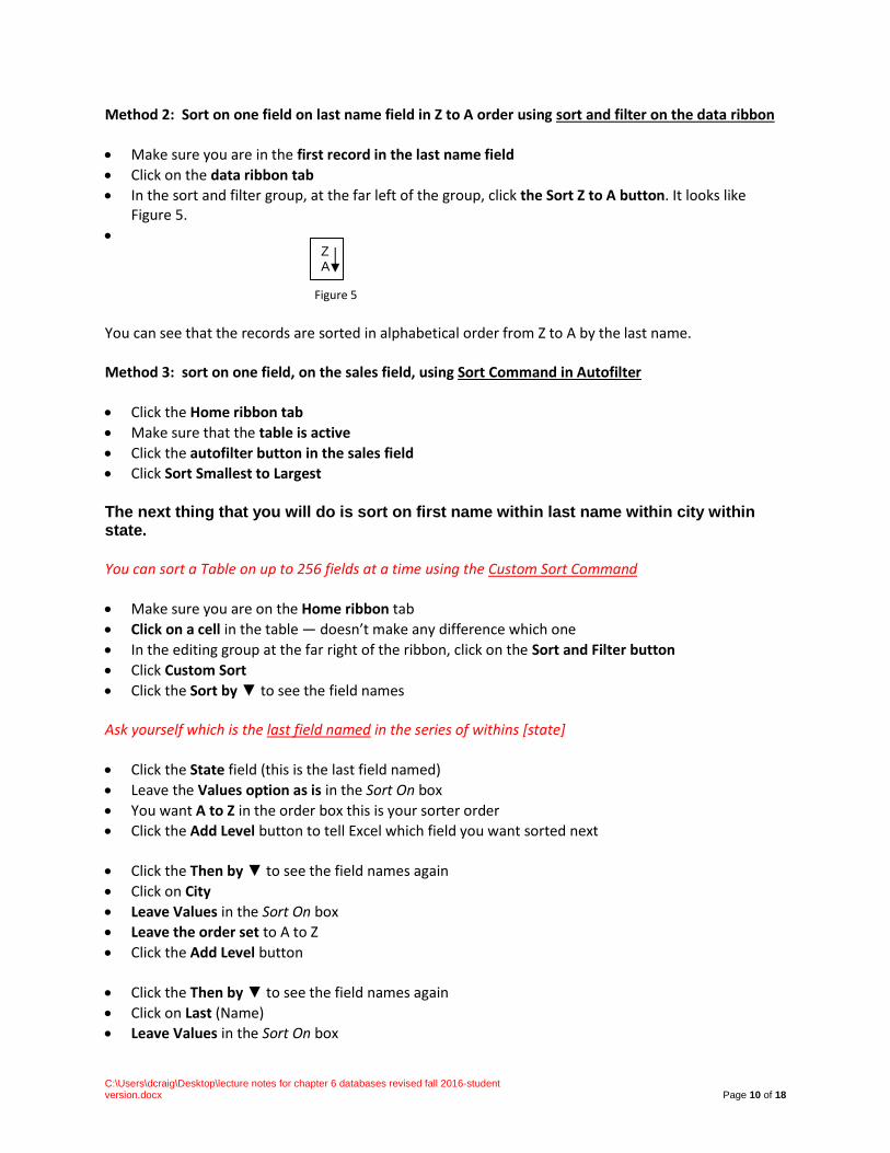
In the sort and filter group, at the far left of the group, click the Sort Z to A button. It looks like Figure 5.

Figure 5 You can see that the records are sorted in alphabetical order from Z to A by the last name. Method 3: sort on one field, on the sales field, using Sort Command in Autofilter

Click the Home ribbon tab

Make sure that the table is active

Click the autofilter button in the sales field

Click Sort Smallest to Largest The next thing that you will do is sort on first name within last name within city within state.

You can sort a Table on up to 256 fields at a time using the Custom Sort Command

Make sure you are on the Home ribbon tab

Click on a cell in the table — doesn’t make any difference which one

In the editing group at the far right of the ribbon, click on the Sort and Filter button

Click Custom Sort

Click the Sort by ▼ to see the field names Ask yourself which is the last field named in the series of withins [state]

Click the State field (this is the last field named)

Leave the Values option as is in the Sort On box

You want A to Z in the order box this is your sorter order

Click the Add Level button to tell Excel which field you want sorted next

Click the Then by ▼ to see the field names again

Click on City

Leave Values in the Sort On box

Leave the order set to A to Z

Click the Add Level button


Click on Last (Name)


Z A



Click the Add Level button


Click on First (name)



Click OK to sort the table Subtotals

Assume you are a sales manager and want to do some sales analysis. You might want to total the sales for each state and then look at each state’s sales in detail. You can only subtotal one field; it is called the control field. You must decide which field you want subtotaled — we will use state—Then you should sort the records so that all the records for each state are together. You have already sorted so that all the states are in groups, so you can do subtotals by state. Converting the records to a range We will start by converting the records into a range instead of a database. This is because the subtotals feature is not available in a table per se, only in a range. When we get done with the subtotaling, we will put the rows of data back into a database.

Right click anywhere in the table

In the shortcut menu, click on Table (about 2/3 of the way down the menu)

Click Convert to Range

Click Yes — notice that the autofilter buttons are gone

Setting up the Subtotaling

Click on the Data ribbon tab

In the outline group at the right of the ribbon, click Subtotal

What do you want at each change in the state? A sum

So… click Sum if necessary

Then you have to decide the fields in which you want the sums (or subtotals)

You can’t sum anything but sales or commissions because they are the only fields with numbers in them, so … deselect grade in the Add subtotal to area

Click the sales and commission fields to designate where you want subtotals

Click OK Outline to hide and unhide data by looking at different levels of summing (all records, state subtotals, grand total)


Dots stand for individual records. Second level minus signs for states means that there are no hidden records in each of the state groups of records. Click 1 at the top of the outline group and examine what is happening Click 2 at the top of the outline group and examine what is happening Click 3 at the top of the outline group and examine what is happening Click back on 2 again Basically, the plus signs mean “more.” In a nutshell, a plus sign indicates that there are records that do not show. There are more records that are hidden.

Click on the plus button for CA and see the detail and minus sign for that state group The minus sign means that there are no more records for this group. No records are hidden.

Click the minus button for CA to close the detail for that state

Click on the plus button for IL and see the detail and minus sign for that state group

Click the minus button for IL to close the detail for that state

Click on the plus button for TX and see the detail and minus sign for that state group

Click the minus button for TX to close the detail for that state

Click on 3 in the outline level buttons With all of the records showing, in the outline group on the ribbon, click the subtotal button to get the subtotal dialog box back

Click Remove all What is the difference between using the outline feature buttons showing 1, 2, and 3 at the top of the side panel and the groups with the + and – ? Using the group feature, you can look at different levels of detail by group at the same time, but with the outline feature, you don’t have that flexibility—you have to display all the information for all the groups at any particular level —no picking and choosing. Click Remove all to remove the subtotals. Putting the Range back into a Table

Select from A6 to H18


In the Styles group, click the Format as Table button

At the very top of the table gallery, click on the format you created

In the little Format as Table dialog box, click OK

Click outside the table


A query is looking for records in a table that meet certain criteria (conditions). Suppose you only want to see the records where the comment is good and the state is CA. Query a Table using Autofilter (filter two fields)

Click inside the table

Click on the autofilter in the state field

Click on (select) All to deselect the states

Click in the box for CA

Click OK—you only see the records for California now, but remember we want to see those in CA with good in the comment field

Click on the autofilter button for comment

Click (select) All to clear all of the check marks

Notice that some of the rows are missing

Click on good

Click OK—only one row shows Showing all of the Records Again

Make sure the table is active by clicking in it

Click the Data ribbon tab

In the sort and filter group, click the filter button (looks like a funnel) Suppose you want to use autofilter to see only those records where sales are between 44,000 and 56,000? You will need to use custom filtering. Custom Filtering with AutoFilter

Click somewhere in the table

In the sort and filter group, click filter again to get the autofilter buttons back

Click the sales autofilter button

Point to the Number Filters on the pull down menu

At the bottom of the fly out menu, click on Custom Filter

Click the ▼ for the first text box

Click on “is greater than or equal to”

Type 44000 in the second text box

Click the ▼ for the second text box on the left

Click on “is less than or equal to”

Click in the second text box on the right and type 56000

Click OK You only see the records where the sales are between 44,000 and 56,000


Click in the table

To get the records back, in the sort and filter group, click the filter button on the ribbon

Now you want to have your filtered (those that met the conditions) records put into a separate area

Setting up the Criteria Range for Advanced Filtering

Select the database title row and the row of field names (A5 to H6)

Ctrl C to copy

Click in A1

Ctrl V to paste

Press Esc

Click in A1 and type Criteria Area Press enter

Setting up the Extraction Range for Advanced Filtering (where the records that are selected will be copied)

Select A5 to H6 again

Ctrl C to copy

Click in A21

Ctrl V to paste

Press Esc

Click in A21, and replace the existing text with Extraction Area

Press enter Suppose you want to see only records for the state of IL AND where the comment is “work with.” When more than one condition must be met in order for the record to be selected, you are said to be anding because the records must meet more than one condition.

Click in D3 and type IL

Click in H3 and type work with

Click inside the table to activate it

Make sure you are on the Data ribbon tab

In the sort and filter group, click on Advanced [may turn off autofilter] and shows the advanced filter dialog box

Change the criteria range from A2 to H3

Click OK

To show all the records again, click in the table to activate it

In the sort and filter group, click Assume you are a sales manager and want to do some sales analysis. You might want to total the sales for each state and then look at each state’s sales in detail. WE just did anding, now we will do ORRING ANDING (more than one condition (criterion) must be met—listed on one row of criteria area ORRING, (only one condition of several has to be met.)—listed on different rows of criteria area


Suppose you want to extract and copy into the extraction area all the records where the state is TX OR the sales are over 50,000 Each row is a set of criteria, so you put TX in the state field on one row in the criteria range and >50000 in the sales field on the next row down in the criteria area Extracting Records (copying selected records to another place in the sheet-orring)

In D3, in the state field, type TX—abbreviation must match, not Texas

In E4, type >50000

Press enter

Delete work with in H3

Click in the table to make it active

In the sort and filter group, click advanced

Click in the copy to another location option

In the Criteria range text box, change H3 to H4

Check the Copy to area and make sure it designates $A$22:$H$22 (extraction area) Click OK

Scroll down to see that the records are all for either TX or over 50,000 Wild Cards and Leaving a blank row in the criteria Area There are two wild cards. One wild card, the question mark, takes the place of a single character. The other, the asterisk (*), takes the place of any number of characters.

Delete all the criteria

In E3, in the sales field, type >45000

In B3, type O* [using a wild card to find all those last names that start with O]

Click in the table to make it active

In the sort and filter group, click advanced

Click in the copy to another location option

We are leaving row 4 blank and in the criteria range on purpose

Check the Copy to area and make sure it designates $A$22:$H$22

Click OK

Scroll down to see that all of the records copied into the extraction area; this is because there was no criteria in row 4 and so all of the records met the condition to be selected.


Fixing the empty criteria row problem

Click in the table

Click advanced

In the criteria range text box, carefully change $H$4 to $H$3

Click in the Copy to another location option Only Ota was extracted Suppose you knew you had employees in Illinois who were named either Ribera or Rivera and wanted to find who they were. The ? Wild Card

Using the single character wild card to search for employees whose names are spelled Ri_era

Delete the existing criteria

Click in B3 and type Ri?era

Click in the table

In the Sort and Filter group, Click Advanced

Click in the Copy to another location option

Click OK You see Ron Ribera and Juan Rivera. Database Functions

You cannot get totals for states with the subtotal function without first sorting the database so that all the records are each state are together. However, with the database functions, you can get totals, averages, etc. by any field with numbers even if the records are not sorted the way they were for subtotals. We will first name the table so that we can refer to it by its name rather than the upper left cell address to the lower right cell address. Select from A6 to H18 Click in the name box and type database as the name, and press enter Click outside of the selected cells Test the name by clicking the name ▼ and clicking on database Select from J12 to O12 Click the Home ribbon tab In the alignment group, click merge and center In the merged cell, type Statistics Area for Database Functions In the Styles group, click Cell styles Click Title Change the font size to 16


Setting up the Criteria Area you will need to do the Database Functions

In J13, type state [all lower case]

In K13, type state [all lower case]

In L13, type state [all lower case]

In M13, type city [all lower case]

In N13, type gender

In O13, type gender

In J14, type CA

In K14, type TX

In L14, type IL

In M14, type Dallas

In N14, type M

In O14, type F

In J17, type Highest sales in California

In J18, type Lowest sales in Illinois

In J19, type Average commission in Texas

In J20, type Total sales for Illinois

In J21, type Number of reps in Dallas

In N17, type =dmax(database,”sales”,K13:K14) [point to range for last argument]

In N18, type =dmin(database,”sales”,L13:L14) [point to range for last argument]

In N19, type =daverage(database,”comm”,K13:K14) [point to range for last argument]

In N20, type =dsum(database,”sales”,L13:L14) [point to range for last argument]

DCOUNT needs a numeric field, so we will use the commission field—in our case, every rep has earned a commission. If a rep had no sales, you would put a zero in for sales; do not leave the cell empty.

In N21, type =dcount(database,”comm”,M13:M14) SUMIF and COUNTIF

Select J23 to O23

In the alignment group, click on merge and center

In the merged cell, type Statistics Area for SUMIF and COUNTIF

In the Styles group, click Cell Styles

Change the font size to 16 or 14 [whichever fits best in the room available]

In J24, type No. of female reps.

In J25, type Total sales of female reps.

Click in N24 and type =countif(F7:F18,”f”)

Press enter

In N25, type =sumif(F7:F18,”f”,E7:E18)

Ctrl S to save the workbook


Use this to Guide You

cis 100 databases in excel creating, sorting, …staff notes for...c:\users\dcraig\desktop\lecture...

Documents