Child Marriage, Weather Shocks, and the Direction ofMarriage Payments∗

Lucia Corno† Nicole Hildebrandt‡ Alessandra Voena §

April 4, 2017

Abstract

Cultural norms play an important role in influencing economic behavior and can shape households’ decisionseven in response to the same economic circumstances. For this reason, they may determine the external validityof the empirical findings from natural experiments. This paper examines the effect of local rainfall shocks onfemale child marriages in sub-Saharan Africa and in India. We show that droughts have similar negative effects oncrop yields, but opposite effects on child marriage in the two regions: in Africa, droughts increase the probabilityof child marriage, while in India droughts decrease such a probability. To explain this outcome, we develop asimple equilibrium model of the marriage market in which income shocks affect the timing of marriage becausethe transfers that traditionally occur at the time of marriage are a source of consumption smoothing, particularlyfor a woman’s family. Exploiting heterogeneity in the marriage payment traditions across countries and ethnicgroups, and additional data from Indonesia, we argue that the differential impact of drought on the marriagehazard that we document is explained by differences in the direction of traditional marriage payments in eachregion, bride price across sub-Saharan Africa and Indonesia and dowry in India.

JEL Codes: J1, O15.Keywords: Income shocks, informal insurance, marriage, Africa, India, dowry, bride price

∗We thank David Atkin, Marianne Bertrand, Bill Easterley, Raquel Fernàndez, Paola Giuliano, Luigi Guiso,Rick Hornbeck, Seema Jayachandran, Sylvie Lambert, Eliana La Ferrara, Nathan Nunn, Yaw Nyarko, DebrajRay, Dean Spears, and participants in presentations at SITE, EUDN, Harvard/MIT, CEPR, AEA meetings,Università Cattolica, Columbia and UCSD for helpful comments. Yin Wei Soon provided outstanding researchassistance.†Catholic University of the Sacred Hearth and IFS. Email: lucia.corno@unicatt.it.‡Boston Consulting Group Email: nhilde1@gmail.com.§The University of Chicago, NBER and CEPR. Email: avoena@uchicago.edu.

1

1 Introduction

Social scientists have now well recognized the important role of cultural and traditional norms

in shaping economic behavior both in developed and in developing countries. Recent studies

have also shown that social norms can contribute to the effectiveness of development policies, and

there have been increasing calls by international organizations, such as the World Bank and the

United Nations, for improving the tailoring of interventions to the local context.1 In this paper,

we argue that cultural norms may also influence the external validity of the empirical findings

from natural experiments, by radically modifying the economic relationship between variables,

and hence that understanding their role can contribute to policy design and evaluation. In

particular, we examine the determinants of female child marriage, a widespread and dramatic

phenomenon in the developing world, and we find that understanding how economic forces

influence it requires also understanding how the local cultural norms work.

Despite improvements in female educational and economic opportunities, large numbers of

young women continue to marry at an early age. Worldwide, more than 700 million women

alive today were married before their 18th birthday and 25 million entered into union before

age 15 (UNICEF, 2014). Child marriage (defined as marriage before the age of 18) is especially

pronounced among women living in sub-Saharan Africa and South Asia, where more than 50%

of women continue to marry before age 18, and 20% marry before age 15.2 Because of the

strong association between child marriage and poverty worldwide, it is natural to ask whether

experiencing negative economic shocks increase the risk that a woman marries before turning

18.

To shed light on this question, we examine the effect of rainfall shocks –a major source

of income variability in rural areas that rely on rain-fed agriculture– on the probability of

early marriage among young women in two regions of the world, sub-Saharan Africa and India.

We combine rainfall data from the University of Delaware Air Temperature and Precipitation

project (UDel) between 1950 and 2010 with marriage data from sixty pooled Demographic and

Health Surveys (DHS) for thirty sub-Saharan African countries between 1994 and 2013, from1The most recent World Development Report focuses on the idea that “paying attention to how humans think

(the processes of mind) and how history and context shape thinking (the influence of the society) can improve thedesign and the implementation of development policies that target human choice and action (behavior)" (WorldBank, 2015).

2Figures are based on DHS surveys for India (2005) and Africa (2006-2012), considering women aged 20-24living in rural areas. See table A2 for the African countries included in the analysis.

2

the 1998-1999 DHS of India, and the 2005 Indian Human Development Survey (IHDS). We

obtain information on the age of marriage and on the history of rainfall shocks of approximately

450,000 women for every year between age ten and age seventeen. To investigate the effect of

rainfall shocks on agricultural output, we also merge the UDel data with historical data on crops

yields provided by Food and Agricultural Organization (FAO) and by the World Bank. In both

regions, a drought, defined as an annual rainfall realization below the 15th percentile of the local

rainfall distribution, is associated with a significant decline in agricultural production.

Our main results indicate that, in these areas, despite having similar effects on crop yields,

droughts have opposite effects on early marriage: while in sub-Saharan Africa these low realiza-

tions increase the hazard of marriage before age 18, we find that in India they reduce such a

hazard. Our main empirical result shows that a drought increases the annual hazard of marriage

between ages 10 and 17 by 0.26 percentage points (3.9 percent) in Sub-Saharan Africa, and it

decreases the hazard of marriage between ages 10 and 10 by 0.69 percentage points (7.8 percent)

in India. These findings are robust to a wide set of changes to the definition of a drought,

and indicate that lower rainfall is broadly associated with more child marriages in Sub-Saharan

Africa and fewer in India. These effects persists for women up to age 25, and influence women’s

fertility as well. In particular, we find that, in Sub-Saharan Africa, a drought is associated with

a 0.19 percentage points (5 percent) increase in the annual probability of having a child before

turning 18.

To interpret this result, we develop an equilibrium model of child marriage in which parents

can choose to time the marriage of their children in order to smooth consumption, because

of the significant transfers of wealth and goods that take place at the time of marriage. In

many countries in Sub-Saharan Africa, it is customary for the groom or his family to pay a

bride price to the bride’s family, whereas in India, the prevailing tradition is for the bride’s

family to pay a dowry to the groom or his family at the time of marriage. During a drought,

families have a higher marginal utility of consumption, and prefer to anticipate (in Sub-Saharan

Africa) and delay (in India) their daughter’s marriage in order to consume the transfer money. In

equilibrium, though, also the grooms’ families are affected by the same aggregate shocks. Hence,

equilibrium marriage prices fall during droughts, and equilibrium quantities vary depending on

which side of the market is more price elastic. Under virilocality, i.e. when a couple lives with

the groom’s family, as is common in our data, child marriages increase under bride price and

3

decrease under dowry in equilibrium, because a man’s parents value the marriage transfer less

if the can rely on their son’s economic support in old age, compared to a woman’s parents, who

are less likely to benefit from a daughter’s support after she is married.

Having documented these empirical patterns in the two regions, we further examine evidence

in the data that supports of our hypothesis. First, we exploit historical data on heterogeneity

in marriage payments across ethnic groups collected by the anthropologist George Peter Mur-

dock’s (1967). Within sub-Saharan Africa, where there is substantial variation in local marriage

payment norms, we show that the positive effect of droughts on the hazard into early marriage

is concentrated in countries that have higher prevalence of ethnic groups that traditionally make

bride price payments at marriage. Even within countries, the ethnic groups that traditionally

engage in bride price payments are the most sensitive to droughts. Second, within India, where

dowry prevails across regions, casts and religious groups, we find that strongest among hindus,

who have an ancient and stronger tradition of dowry payments.

Examining the characteristics of couples that match during droughts, opposite patterns arise

in the two economies. In Sub-Saharan Africa, low-educated women who end up having lower

decision-making power in their household are more likely to marry during droughts, while in

India, high-educated women who end up having higher say in household decision making are more

likely to marry during droughts. Examining data from the Rural Economic and Demographic

Survey (REDS), we find that dowries paid for marriages that occur during droughts are twenty

percent lower than those paid during normal times, consistently with our model.

Finally, we further verify our findings by bringing additional evidence from Indonesia, a

country within Asia, like India, but with a large number of ethnic groups traditionally practicing

bride price payment and significant variation in the virilocal norm (Ashraf, Bau, Nunn, and

Voena, 2016; Bau, 2016). Interestingly, the effects that we find in this country are comparable

to the ones documented in Sub-Saharan Africa: household exposed to rainfall shock have a higher

probability of child marriage. As predicted by our model, the effect is driven by communities

that traditionally engage in bride price payments and that have a virilocal tradition.

Our paper is related to two broad strands of the economics literature. First, it fits in the broad

body of research on the importance of culture and institutions in shaping economic behavior.

Much of this work has looked at the role of cultural values and beliefs, such as trust, family ties,

and preferences about women’s role, on economic development (Fernandez, Fogli, and Olivetti,

4

2004; Fernandez and Fogli, 2009; Algan and Cahuc, 2010; Alesina, Algan, Cahuc, and Giuliano,

2010; Tabellini, 2010; Nunn and Wantchekon, 2011). A growing part of this literature has

explored the influence of traditional social norms - behaviors that are enforced through social

sanctions - on economic behavior (Bhalotra, Chakravarty and Gulesci, 2016; Platteau, 2000).

For example, La Ferrara (2007) and La Ferrara and Milazzo (2012) test the implication of the

matrilineal inheritance rule on inter-vivos transfer and on human capital accumulation in Ghana,

where the largest ethnic group is traditionally matrilineal. In the domain of traditional marriage

practices, Jacoby (1995) studies the effect of polygyny on women agricultural productivity and

find that, conditional on wealth, men do have more wives when women are more productive.

Tertilt (2005) shows that banning polygyny lowers fertility and shrinks the spousal age gap in

sub-Saharan Africa. While marriage payments –dowry and bride price– are widespread in many

regions in Africa and Asia only few studies have looked at their effect on household’s economic

decision. In a recent paper, Ashraf, Bau, Nunn, and Voena (2016) show that ethnic groups that

traditionally engage in bride price payment at marriage in Indonesia and Zambia are more likely

to see female enrollment increase in response to a large expansion in the supply of schools. In

those communities, higher female education at marriage is associated with a higher bride price

payment received thus providing a greater incentive for parents to invest in girls’ education.

Second, our results contribute to the large economic literature that studies the coping mech-

anisms used by poor households to deal with income risk. Despite imperfect markets for formal

insurance, credit, and assets, rural households seem well-equipped to smooth consumption in the

face of short-term, idiosyncratic income shocks, often through informal insurance arrangements

(see Townsend (1994), Dercon (2002), De Weerdt and Dercon (2006), Fafchamps and Gubert

(2007) and Angelucci, De Giorgi, Rangel, and Rasul (2010) among others). However, in the

face of aggregate shocks, households must rely on a different set of strategies to cope (Dercon,

2002). These strategies, which include migration (Morten, 2016), off-farm employment, and

liquidation of buffer stock (Fafchamps, Udry, and Czukas, 1998), are typically unable to provide

full consumption smoothing. This challenge is illustrated in the growing empirical literature

looking at the impact of negative rainfall shocks on individual outcomes, which has identified

negative effects of drought on infant and child health, schooling attainment and cognitive test

score performance, increased rates of domestic violence and violence against women, and even

5

higher rates of HIV infection (Burke, Gong, and Jones, 2014).3 In this paper, we show that

adjusting the timing of marriage is another strategy that households use to cope with aggregate

variation in income, which can have harmful long-run welfare implications for young women.

The remainder of the paper proceeds as follows. Section 2 provides background information

on marriage markets, marriage payments, and early marriage in India and Africa. Section 3

illustrates the equilibrium model. Section 4 describes the data used in the analysis, and Section

5 explains the empirical and identification strategy. Sections 6 and 7 summarize the results and

provide robustness checks. Section 8 concludes.

2 Background

Early marriage and marriage payments are both widespread practices in developing coun-

tries, particularly in sub-Saharan Africa and in South Asia.

2.1 Early marriage

Early marriage is still a dramatic practice in many countries around the world. The practice

is associated with a wide range of adverse outcomes for women and their offspring, including

higher rates of domestic violence; harmful effects on maternal, newborn, and infant health; re-

duced sexual and reproductive autonomy; and lower literacy and educational attainment (Jensen

and Thornton, 2003; Field and Ambrus, 2008). Based on these findings, international organi-

zations such as UNICEF and the World Bank have called for “urgent action", arguing that the

eradication of early marriage is a necessary step towards improving female agency and autonomy

around the world.4

The reasons why the practice persists are numerous and inter-related. Parents often view

early marriage as a socially acceptable strategy to protect their daughter against events (i.e.

sexual assault, out-of-wedlock pregnancy, etc.) that could compromise her purity and subsequent

marriageability (see for example Worldvision 2013; Bank 2014). Grooms also tend to express a

preference for younger brides, purportedly due to beliefs that younger women are more fertile,

more likely to be sexually inexperienced and easier to control (Field and Ambrus, 2008).3See Dell, Jones, and Olken (2013) for a comprehensive review of this literature.4See “No time to lose: New UNICEF data show need for urgent action on female genital mutilation and child

marriage", UNICEF Press Release, 22 July 2014.

6

Although cultural and social norms are considered important drivers of the persistence of

early marriage, economic conditions also play a role. Girls from poor households are almost

twice as likely to marry early as compared to girls from wealthier households (Bank, 2014). This

effect is compounded by the tradition of marriage payments (dowry and bride price) in Africa

and in India. In India, the prevailing tradition is for the parents of the bride to pay a dowry to

the groom’s family at the time of marriage, while in Africa, bride price is traditionally paid by

the groom to the parents of the bride. The available empirical evidence indicates that dowry is

increasing in bride’s age, while bride price is at first increasing and then rapidly decreasing in

bride’s age, meaning that under both customs, marrying a daughter earlier can be financially

more attractive for her parents.5

2.2 Marriage payments

The prevailing economic view of marriage payments is based on the seminal work of Becker

(1991). Individuals enter into the marriage market to find the match that maximizes their

expected utility; the marriage market matches partners and determines the division of surplus

between them. Given this characterization, marriage payments (dowries and bride prices) may

emerge as pecuniary transfers that serve to clear the marriage market. Different types of marriage

payments can emerge in response to scarcity on one side of the marriage market: when grooms

are relatively scarce, brides pay dowries to grooms, and when brides are relatively scarce, grooms

pay bride prices to brides. Alternatively, payments can arise as the transfers to equilibrate the

market when the rules for division of household output are inflexible, so that a spouse’s shadow

price in the marriage market differs from his or her share of household output. In cases where

the woman’s shadow price on the marriage market is less than her share of household output, a

bride price will emerge to encourage her to marry; in the opposite case, when a woman’s shadow

price on the marriage market is more than her share of household output, dowries will emerge

to encourage male participation on the market.6

5For evidence on the relationship between dowry and bride’s age in India, see Chowdhury (2010). Arunachalamand Naidu (2010) study the relationship between fertility and dowry. Empirical data on bride price is very limited,but for evidence on bride price and bride’s age in the Kagera Health and Development Survey from Tanzania,see Corno and Voena (2016).

6Traditionally, dowry appears to have served mainly as a pre-mortem bequest made to daughters rather thanas a payment used to clear the marriage market (Goody and Tambiah, 1973). However, with development, dowryappears to have taken on a function more akin to a groomprice, a price that brides’ parents must pay in orderto ensure a husband for their daughter. The transition of the property rights over dowry from the bride to herhusband is studied in Anderson and Bidner (2015), who document a similar transition in late-middle ages in

7

There is an important difference between marital customs in sub-Saharan Africa and India:

in Africa, bride price is the prevailing norm, while in India, dowry is the most common practice.

Traditionally, the practices of bride price was near-ubiquitous across the sub-Saharan African

sub-continent: more than than 90% of ethnic groups in sub-Saharan Africa traditionally paid

bride price (Goody, 1976; Murdock, 1967). This practice is not universal in contemporary Africa,

but it remains a substantial transfer across the region (see appendix table ). For example, a

household panel survey conducted in Zimbabwe in the mid-1990s revealed near-universality of

bride price at the time of marriage; average bride wealth in this data (received primarily in the

form of heads of cattle) was estimated to be two to four times a household’s gross annual income

(Decker and Hoogeveen, 2002). Relying on DHS data, Anderson (2007) reports that bride price

was paid in about two-thirds of marriages in rural Uganda in the 1990s, down from 98% in

the period between 1960-1980 and 88% from 1980-1990. In a large-scale survey conducted by

Mbaye and Wagner (2013) in rural Senegal in 2009-2011, bride price was found to have been

paid in nearly all marriages. Ashraf, Bau, Nunn, and Voena (2016) document that the practice

is widespread in modern-day Lusaka (Zambia), with payments often exceeding annual per capita

GDP.

The pioneering work on dowry in economics has focused on historical data from Europe

(Botticini, 1999; Botticini and Siow, 2003). In contemporary India, dowry is paid in virtually all

marriages (Anderson, 2007). Interestingly, although dowry has been practiced in Northern India

for centuries, it is a much more recent phenomenon in the South, where bride price traditions

were formerly the norm. The transition from bride price to dowry began in the start of the

20th century, and has been attributed to an increasingly skewed sex ratio (more potential brides

than potential grooms), which has increased competition among women for grooms, particularly

educated young men with urban jobs (Caldwell, Reddy, and Caldwell, 1983). Some authors have

argued that dowry payments have grown substantially over the first half of the twentieth century,

a phenomenon which has been explained by slowing population growth, or as hypergamy and

the caste system (Anderson, 2003; Rao, 1993; Sautmann, 2012). Edlund (2006), however, argues

that actual net dowries have experienced little change. Over the period we study in our data,

dowry is widespread across India and payments are large in magnitude (often significantly above

Europe. The view of dowry as a pre-mortem bequest to daughters is also at odds with the prevalence of dowryviolence in India, whereby grooms threaten domestic violence in order to get higher transfers from their wife’sparents (see Bloch and Rao (2002); Sekhri and Storeygard (2013)).

8

average household income).

There are numerous explanations proffered to explain the existence of dowry in India and

bride price in Africa. Goody and Tambiah (1973) explain the prevalence of bride price in Africa

by the continent’s land abundance and low population density. The relative scarcity of labor

requires men to compensate the bride’s family for losing her labor, and increases the value of the

woman’s ability to produce offspring. In contrast, in South Asia where population density is high

and land is scarce, men are distinguished by their land holdings, and women’s own labor and

ability to reproduce is relatively less valued. Boserup (1970) offers a slightly different hypothesis

based on differences in women’s agricultural productivity in the two regions. She argues that

in Africa, which has a non-plough agricultural system, female labor is more important than in

Asia, a region characterized by plough architecture, and this generates marriage payments to

move towards the bride’s side of the market. This hypothesis finds empirical support in Giuliano

(2014) who documents a positive correlation between women’s role in agriculture and marriage

payments and has also been used to explain cross-cultural differences in beliefs on the role of

women in society (Alesina, Giuliano, and Nunn, 2013).

3 Theoretical framework

In this section, we develop a simple equilibrium model where aggregate economic fluctuations

affect child marriage decisions by families. Marriage payments play a crucial role and their

direction determines whether more or fewer women marry early when aggregate income is low.

Below, we present a version of the model with logarithmic utility and a uniform distribution

of income heterogeneity. In Appendix C, we extend this framework in two ways. First, we study

how the presence of child labor, and the effect of droughts on children’s wages, interacts with

the marriage market and the marriage payments. Second, we extend this model to more general

utility functions and distributions of the heterogeneity, showing that our propositions are valid

under milder assumptions than the one presented her.

3.1 Setup

There is a unit mass of households with a daughter and a unit mass of households with a son.

There are two periods, which correspond to two life stages, childhood (t = 1) and adulthood

9

(t = 2).

In each period, household income depends on adult children’s contributions and on an aggre-

gate realization of weather, which can take values yt ∈ yL, yH, with yL < yH , each occurring

with equal probability independently in every period, plus an idiosyncratic realization εt which

is distributed uniformly on [0, 1]. Hence, in period t, the total income of a household i with an

adult daughter is equal to yt+εit+wf , where wf is a woman’s contribution to the household bud-

get. Following Boserup’s (1970) interpretation of the historical origins of marriage payments, we

consider historical wf to be either positive or negative depending on the available technology in

the local community: wf > 0 then generate bride price payment, while a dowry system emerges

when wf < 0. The total income of a household j with an adult son is equal to yt + εjt +wm. The

discount factor is denoted by δ.

The society is patrilocal, and hence upon marriage women move to the groom’s family and

contribute to its budget. In addition, with marriage, the groom’s family acquires offspring, which

deliver utility ξm > 0. There is also a potential utility gain of a woman’s family stemming from

marrying off a daughter (i.e. stigma associated with non-married women), denoted as ξf ≥ 0.

3.2 Adulthood

We define τt > 0 a payment from the groom’s family to bride’s family (bride price) and

τt < 0 a payment from the bride’s family to the groom’s family (dowry). In adulthood, marriage

occurs if both parties prefer it to remaining single. A transfer may be needed to achieve such

an outcome: this implies that there exists a τ ∗2 that satisfies

ln(y2 + εi2 + τ ∗2 ) + ξf ≥ ln(y2 + εi2 + wf )

ln(y2 + εj2 + wm + wf − τ ∗2 ) + ξm ≥ ln(y2 + εj2 + wm).

When income is sufficiently low, the bounds on τ ∗2 require a payment to take place even for

the richest families. In sub-Saharan Africa, with historical wf > 0, a bride price payment is

necessary to persuade women’s parents to let their daughters marry, meaning that

ln(yH + 1 + wf ) > ln(yH + 1) + ξf .

10

In India, where historically wf < 0, a dowry payment is necessary to persuade men to support

a bride into their household:

ln(yH + 1 + wm) > ln(yH + 1 + wm + wf ) + ξm.

These conditions imply that a lower bound on the marriage payment is equal to τ 2 =

1−exp(ξf )exp(ξf )

(y2 + εi2) + wf

exp(ξf ), while the upper bound is τ2 = exp(ξm)−1

exp(ξm)(y2 + εj2 + wm) + wf . In

what follows, we assume that there exists a payment τ ∗2 ∈ [τ 2, τ2]. One simple example of

equilibrium is that men make a take-it-or-leave-it offer to the woman’s parents, and the parents

decide whether or not to accept. For example, when ξf = 0, men offer τ ∗2 = wf . Hence, whenever

wf < 0, the transfer is a dowry, i.e. a payment from the bride’s family to the groom’s family,

while with wf ≥ 0, the payment is a bride price, i.e., a payment from the groom’s family to the

bride’s family.

Following Boserup’s interpretation, the direction of the marriage payment may be due to

the historical sign of wf , but in what follows, we do not impose that present-day wf has to

differ across areas of the world. In this sense, the fact that marriage payments are the way by

which the marriage markets clear and whether in adulthood grooms’ families (τ2 > 0) or brides’s

families (τ2 < 0) make such payments are cultural norms in this model, intended as a way of

selecting among multiple equilibria (Greif, 1994).

Given the payment τ ∗2 , payoffs from marrying in the second period are:

ln(y2 + εj2 + wm + wf − τ ∗2 ) + ξm and ln(y2 + εj2 + τ ∗2 ) + ξf .

If a couple is already married when entering the second period, the families’ payoffs instead

are

ln(y2 + εj2 + wm + wf ) + ξm and ln(y2 + εi2).

3.3 Childhood

In the first period, parents decide whether or not to have their children marry. For a given

transfer τ1 paid in marriages that occur in the first period, payoffs are the following.

11

If marriage occurs:

ln(y1 + εj1 − τ1) + δE[ln(y2 + εj2 + wm + wf ) + ξm

]ln(y1 + εi1 + τ1) + δE

[ln(y2 + εi2) + ξf

].

Instead, if marriage is delayed:

ln(y1 + εj1) + δE[ln(y2 + εj2 + wf − τ ∗2 + wm) + ξm

]ln(y1 + εi1) + δE

[ln(y2 + εi2 + τ ∗2 ) + ξf

].

A woman from household i will get married in the first period if and only if:

ln(y1 + εi1 + τ1)− ln(y1 + εi1) ≥ δE[ln(y2 + εi2 + τ ∗2 )

]− δE

[ln(y2 + εi2)

]A man from household j will get married in the first period if and only if:

ln(y1 + εj1 − τ1)−ln(y1 + εj1) ≥

δE[ln(y2 + εj2 + wm + wf − τ ∗2 )

]− δE

[ln(y2 + εj2 + wm + wf )

].

Define the right handside terms as Ωf = δE [ln(y2 + εi2 + τ ∗2 )− ln(y2 + εi2)] and

Ωm = δE[ln(y2 + εj2 + wm + wf − τ ∗2 )− ln(y2 + εj2 + wm + wf )

]. For simplicity, define alsoHf =

exp(Ωf ) and Hm = exp(Ωm).

3.3.1 Demand and supply for brides in sub-Saharan Africa

When τ ∗2 > 0, Ωf > 0 and Hf > 1. Also Ωm < 0 and hence Hm < 1.

For a given τ1, define a marginal household with daughter i such that:

ln(y1 + εf∗1 + τ1)− ln(y1 + εf∗1 ) = Ωf

Given the expression above, there exists a threshold income shock for women’s parents such

that, when εit < εf∗(τ1), parents will want their daughter to marry in the first period. Hence,

because of the uniform assumption, a measure εf∗ of women wants to get married. The supply

12

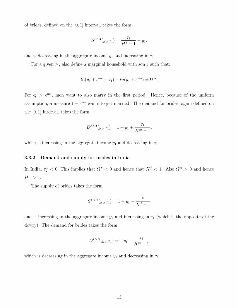
of brides, defined on the [0, 1] interval, takes the form

SSSA(y1, τ1) =τ1

Hf − 1− y1.

and is decreasing in the aggregate income y1 and increasing in τ1.

For a given τ1, also define a marginal household with son j such that:

ln(y1 + εm∗ − τ1)− ln(y1 + εm∗) = Ωm.

For εjt > εm∗, men want to also marry in the first period. Hence, because of the uniform

assumption, a measure 1− εm∗ wants to get married. The demand for brides, again defined on

the [0, 1] interval, takes the form

DSSA(y1, τ1) = 1 + y1 +τ1

Hm − 1,

which is increasing in the aggregate income y1 and decreasing in τ1.

3.3.2 Demand and supply for brides in India

In India, τ ∗2 < 0. This implies that Ωf < 0 and hence that Hf < 1. Also Ωm > 0 and hence

Hm > 1.

The supply of brides takes the form

SIND(y1, τ1) = 1 + y1 −τ1

Hf − 1

and is increasing in the aggregate income y1 and increasing in τ1 (which is the opposite of the

dowry). The demand for brides takes the form

DIND(y1, τ1) = −y1 −τ1

Hm − 1

which is decreasing in the aggregate income y1 and decreasing in τ1.

13

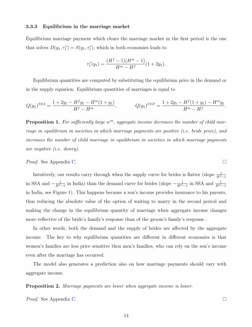
3.3.3 Equilibrium in the marriage market

Equilibrium marriage payment which clears the marriage market in the first period is the one

that solves D(y1, τ∗1 ) = S(y1, τ

∗1 ), which in both economies leads to

τ ∗1 (y1) =(Hf − 1)(Hm − 1)

Hm −Hf(1 + 2y1).

Equilibrium quantities are computed by substituting the equilibrium price in the demand or

in the supply equation. Equilibrium quantities of marriages is equal to

Q(y1)SSA =1 + 2y1 −Hfy1 −Hm(1 + y1)

Hf −Hm, Q(y1)IND =

1 + 2y1 −Hf (1 + y1)−Hmy1

Hm −Hf.

Proposition 1. For sufficiently large wm, aggregate income decreases the number of child mar-

riage in equilibrium in societies in which marriage payments are positive (i.e. bride price), and

increases the number of child marriage in equilibrium in societies in which marriage payments

are negative (i.e. dowry).

Proof. See Appendix C.

Intuitively, our results carry through when the supply curve for brides is flatter (slope 1Hf−1

in SSA and − 1Hf−1

in India) than the demand curve for brides (slope − 1Hm−1

in SSA and 1Hm−1

in India, see Figure 1). This happens because a son’s income provides insurance to his parents,

thus reducing the absolute value of the option of waiting to marry in the second period and

making the change in the equilibrium quantity of marriage when aggregate income changes

more reflective of the bride’s family’s response than of the groom’s family’s response .

In other words, both the demand and the supply of brides are affected by the aggregate

income. The key to why equilibrium quantities are different in different economies is that

women’s families are less price sensitive then men’s families, who can rely on the son’s income

even after the marriage has occurred.

The model also generates a prediction also on how marriage payments should vary with

aggregate income.

Proposition 2. Marriage payments are lower when aggregate income is lower.

Proof. See Appendix C.

14

This finding, particularly in the case of Sub-Saharan Africa, is in line with the literature on

firesales, in which assets are liquidated at lower prices during recessions (Shleifer and Vishny,

1992). Here, droughts are associated with low aggregate output, which is associated with lower

prices irrespectively of the direction of the payments.

4 Data and descriptive statistics

We next describe the different sources of data we exploit to test the predictions of our model.

All datasets used in the analysis are summarized in Appendix table A1.

4.1 Marriage data

Our first key variable is a woman’s age at first marriage. To calculate that we use data from

the Demographic and Health Surveys (DHS) for sub-Saharan Africa and from the DHS and

India Human Development Survey (IHDS) for India.7 For sub-Saharan Africa, we assembled all

DHS surveys between 1994 and 2013 where geocoded data are available, resulting in a total of 72

surveys across 30 countries. In these surveys, GPS data consist of the geographical coordinates

of each DHS cluster (group of villages or urban neighborhoods) in the sample. The list of African

countries and survey waves included in the analysis is reported in the Appendix table A2.

For India, we use the DHS survey from 1998 and the IHDS survey from 2004-05. The two

Indian surveys do not contain GPS coordinate information; instead, they provide information on

each woman’s district of residence, which we can use to match the data to weather outcomes.8

Across all the surveys, the information on woman’s age at first marriage is collected retro-

spectively during the woman’s interview: women are asked to recall the age, month and year

when they were first married.9 The main difference across the surveys is the universe of women

that is sampled for the female interview. In the DHS surveys from Africa, all women in the7DHS surveys are nationally-representative, household-level surveys carried out in developing countries around

the world. The DHS program is funded by USAID, and has been in existence since the mid-1980s. The IndiaHuman Development survey is a nationally-representative, household-level survey first carried out in 2004-05. Asecond wave was held in 2011-12, but it features primarily panel information on the married women who werealready interviewed in the previous wave, and hence does not add a significant number of observations to the2005 sample.

8The DHS India surveys are also referred to as the National Family Health Surveys (NFHS). There are twoadditional DHS surveys available for India: one conducted in 1992, and one conducted in 2005, but they do notprovide information on women’s district of residence: this is why we complement our Indian dat with the IHDSinstead.

9The India DHS does not ask the month of first marriage.

15

household between the ages of 15 and 49 are interviewed. In contrast, in the DHS surveys from

India, all ever-married women aged 15-49 in the household are interviewed; and in the IHDS,

only one ever-married woman aged 15-49 is interviewed in each household. In order to ensure

comparability across surveys and avoid bias resulting from the omission of never-married women

in the sample from India, we limit our analysis to women who are at least 25 years old at the

time of the interview. By this point, most women are married (87% in our African sample),

contributing to the comparability of the two samples. To look at comparable cohorts across the

two sets of surveys, we focus on women born between 1950 and 1989. Furthermore, in the light

of the evidence on rainfall and intensity of civil conflict (Miguel, Satyanath, and Sergenti, 2004),

we exclude women exposed to major civil conflicts. To do so, we use data from UCDP/PRIO

Armed Conflict Dataset on the onset and end of main conflicts in Sub-Saharan Africa in our

sample period, as detailed in Appendix table A3.

As reported in table 1 Panel A, our final sample consists of about 340,000 women in sub-

Saharan Africa, and 97,000 women in India. Figure 2 plots the distribution of ages of marriage

in our data. We consider women who marry from age 10 onward. In both regions, the hazard

into early marriage is relatively low up until age 13 or 14, which is consistent with the finding

that girls are often considered to be ready to marry at the onset of puberty, that usually occurs

sometime in the early teenage years (Field and Ambrus, 2008). The mean age at first marriage

is low, 16.5 years in India and 17.4 years in Africa, and a significant fraction of women are

marrying before age 18 (66.4% and 56.3% in India and Africa, respectively).

4.2 Weather data and construction of weather shocks

To test how income shocks affect the early marriage hazard for young women, we follow an

approach that is widely used in the literature, exploiting variation in local rainfall as a proxy

for local economic conditions. The appeal of this approach is that rainfall is an exogenous event

that has meaningful effects on economic productivity in rural parts of Africa and India, where

most households rely heavily on rain-fed agriculture for their economic livelihood (Jayachandran,

2006; Schlenker and Lobell, 2010; Burke, Gong, and Jones, 2014; Shah and Steinberg, 2016).

Negative rainfall shocks (i.e. droughts), in particular, tend to suppress agricultural output,

which has deleterious effects on households’ incomes.

We use rainfall data produced by geographers at the University of Delaware (“UDel data")

16

to construct rainfall shock measures that capture anomalously high and low rainfall realizations

relative to what is typically experienced in a particular location. The UDel dataset provides

estimates of monthly precipitation on a 0.5 x 0.5 degree grid covering terrestrial areas across

the globe, for the 1900-2010 period.10 For Africa, we use the GPS information in the DHS

data to match each DHS cluster to the weather grid cell and calculate rainfall shocks at the

grid cell level. Our main sample matches up to 2,767 unique grid cells across the sub-Saharan

African region, each of which is approximately 2,500 square kilometers in area. For India, the

lack of GPS coordinate information prevents us from using the same approach. Instead, we use

a mapping software to intersect the UDel weather grid with a district map for India, and then

calculate land-area weighted average rainfall estimates for each district. Of the 675 districts in

India, 502 are represented in our main sample, and these districts have a mean area of 5,352

square kilometers.

The existing economic literature implements a wide variety of methodologies to construct

measures of relative rainfall shocks. Here, we adapt an approach used by Burke, Gong, and Jones

(2014) and define a drought as calendar year rainfall below the 15th percentile of a location’s

(grid cell or district) long-run rainfall distribution. We use a long-run time series (1960-2010)

of rainfall observations to fit a gamma distribution of calendar year rainfall for each location

(grid cell or district). We then use the estimated gamma distribution for a particular location to

assign each calendar year rainfall realization to its corresponding percentile in the distribution.

By constructing rainfall shocks in this manner, we address two important requirements

needed for the validity of our study. First, our rainfall shock measures must have a mean-

ingful economic impact on household incomes. Second, the shock measures must be orthogonal

to other factors that also affect marriage decisions, such as the general level of poverty in an

area, access to schooling and, more general, economic opportunities for young women. The

first condition is essential to ensuring that rainfall shocks are an appropriate proxy for local

economic conditions, while the second condition limits concerns about a spurious relationship

between weather shocks and the early marriage hazard. To provide further confidence that we

have satisfied the first condition, we next investigate the relationship between our constructed100.5 degrees is equivalent to about 50 kilometers at the equator. The rainfall estimates in the UDel data

are based on climatologically-aided interpolation of available weather station information and are widely reliedupon in the existing economic literature (see for example Dell, Jones, and Olken (2012); Burke, Gong, and Jones(2014)). For a detailed overview of the UDel data and other global weather data sets, see Dell, Jones, and Olken(2013).

17

rainfall shock measures and agricultural yields in Africa and India.

By examining realizations that have the same probability that occur in any cell or district (a

percentile of the local rainfall distribution), we limit concerns regarding the correlation between

rainfall shocks and unobserved local characteristics. In figure B1 we plot the percentage of grid

cells (for SSA) and districts (for India) exposed to drought in each calendar year. Given that

droughts are defined as a variation in rainfall below the 15th percentile, the average probability

of experience a shocks in each region is around 15%. Most importantly, figure B1 provides

evidence that our rainfall shock measures are orthogonal to long-run rainfall trends, thus limiting

the concern of a spurious relationship driving our results.

4.3 Weather shocks and crop yields

While the relationship between weather shocks and agricultural output is well established

in the literature (see for example, Jayachandran (2006); Schlenker and Lobell (2010); Shah and

Steinberg (2016); Burke, Gong, and Jones (2014)), in this section we explore how our constructed

measure of rainfall shocks affects aggregate crop yields in Africa and India. To do so, we combine

the rainfall data with yield data, which are available annually for each country in sub-Saharan

Africa over the period 1960-2010 from the FAOStat and for India over the 1957-1987 period

from the World Bank India Agriculture and Climate Data Set.

For Africa, we estimate the impact of rainfall shocks on yields of the main staple crops

growing in the continent: maize, sorghum, millet, rice, and wheat. We also estimate the impact

of shocks on yields for all the natural logarithm of the cereals available in our dataset (which

includes maize, rice, wheat, sorghum, millet plus barley, rye, oats, buckwheat, fonio, triticale and

canary seeds). Since we have country-level yield data, we construct measures of country-level

droughts in the same manner used in the main analysis.

As shown in table 2, droughts (rainfall below the 15th percentile) reduce maize, rice, wheat,

sorghum and millet yield both throughout the set of sub-Saharan African countries available in

the FAO database (columns 1-6) and also by focusing on the 30 countries part of our sample

(columns 7-12). In particular, droughts reduce average cereals yields by 12 percent.

Similarly, for India, we rely on district-level yield data from the World Bank, which has

the great advantage of providing crop yields by district. We look at the impact of rainfall

shocks (constructed at the district-level) on the natural logarithm of the yields of the five most

18

important crops in the country (rice, wheat, jowar, maize and bajra), as well as on all the staple

crops in the districts in our sample (rice, maize, wheat, bajra, sesamum, ragi, jowar, sunflower).

As reported in 3, droughts negatively affects yields of all crops, and reduce average yields by

16% overall.

These finding are supported by the results in A1 and A2, where we plot the coefficients for

dummies for each vingtile of the rainfall realization on the natural logarithm of crop yields, to

explore the relationship between rain and yields across the distribution of rainfall realizations.

While low rainfall is clearly associated with low output, it is harder to identify a clear positive

relationship between high rainfall and output, at least in the coarse units of observation. In

particular, high rainfall appears to positively associated with output for rice, especially in India.

We conclude that our drought measure serves as a strong proxy for a negative output shock in

both regions, while floods are an inconsistent proxy for income, as their effect varies dramatically

depending on the underlying crop.

5 Empirical strategy

To examine the impact of weather shocks on the incidence of early marriage, we estimate a

simple duration model, adapted from Currie and Neidell (2005). Below we discuss our baseline

specification and potential threats to identification.

5.1 Main specification

The duration of interest is the time between t0, the age when a woman is first at risk of

getting married, and tm, the age when she enters her first marriage. In our analysis, t0 is age

10, which is the minimum age at which a non-negligible number of women in our sample report

getting married for the first time.

We convert our data into person-year panel format. A woman who is married at age tm is

treated as if she contributed (tm− t0 + 1) observations to the sample: one observation for each

at-risk year until she is married, after which she exits the data. We merge this individual-level

data to the marriage data according to the year of the rainy season most likely to precede the

potential marriage season. In Sub-Saharan Africa, where there is typically one rainy season in

the fist half of the year and one in the second half, and where marriages occur rather uniformly

19

throughout the year according to DHS data, we consider the calendar year in which a woman

is age t. In India, where 70% of marriages in our IHDS data occur in the first half of the year,

and where the monsoon season is in the second half of the year, we consider rainfall in the year

preceding the one in which the woman is age t.

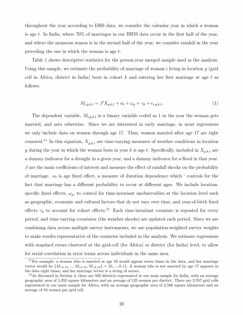
Table 1 shows descriptive statistics for the person-year merged sample used in the analysis.

Using this sample, we estimate the probability of marriage of woman i living in location g (grid

cell in Africa, district in India) born in cohort k and entering her first marriage at age t as

follows:

Mi,g,k,t = β′Xg,k,t + αt + ωg + γk + εi,g,k,t. (1)

The dependent variable, Mi,g,k,t is a binary variable coded as 1 in the year the woman gets

married, and zero otherwise. Since we are interested in early marriage, in most regressions

we only include data on women through age 17. Thus, women married after age 17 are right

censored.11 In this equation, Xg,k,t are time-varying measures of weather conditions in location

g during the year in which the woman born in year k is age t. Specifically, included in Xg,k,t are

a dummy indicator for a drought in a given year, and a dummy indicator for a flood in that year.

β are the main coefficients of interest and measure the effect of rainfall shocks on the probability

of marriage. αt is age fixed effect, a measure of duration dependence which ‘ controls for the

fact that marriage has a different probability to occur at different ages. We include location-

specific fixed effects, ωg, to control for time-invariant unobservables at the location level such

as geographic, economic and cultural factors that do not vary over time, and year-of-birth fixed

effects γk to account for cohort effects.12 Each time-invariant covariate is repeated for every

period, and time-varying covariates (the weather shocks) are updated each period. Since we are

combining data across multiple survey instruments, we use population-weighted survey weights

to make results representative of the countries included in the analysis. We estimate regressions

with standard errors clustered at the grid-cell (for Africa) or district (for India) level, to allow

for serial correlation in error terms across individuals in the same area.11For example, a woman who is married at age 16 would appear seven times in the data, and her marriage

vector would be Mi,k,10, ...,Mi,k,15,Mi,k,16 = 0, ..., 0, 1. A woman who is not married by age 17 appears inthe data eight times, and her marriage vector is a string of zeroes.

12As discussed in Section 4, there are 502 districts represented in our main sample for India, with an averagegeographic area of 5,352 square kilometers and an average of 125 women per district. There are 2,767 grid cellsrepresented in our main sample for Africa, with an average geographic area of 2,500 square kilometers and anaverage of 84 women per grid cell.

20

With the inclusion of location (grid cell or district) and year of birth fixed effects, the impact

of weather shocks on the early marriage hazard is identified from within-location and within year

of birth variation in weather shocks and marriage outcomes. The key identifying assumption of

the analysis is that, within a given location and year of birth, the weather shocks included in

Xg,k,t are orthogonal to potential confounders. Each area is equally likely to have experienced a

shock in any given year, so identifying variation comes from the random timing of the shocks.

The exogeneity of rainfall shocks is particularly important in our setting because, given the

retrospective nature of our analysis, there are many unobservables for which we cannot control

for. Most importantly, we lack data on parental wealth or poverty status around the time of a

woman’s marriage, on the educational background of her parents, and on the numbers and ages

of her siblings, all of which will affect marital timing decisions (Vogl, 2013).

5.2 Threats to identification

A potential threat to identification comes from the fact that we are considering weather

shocks in the place of residence at the time of the survey. Indeed, in all our sources of data, we

only have information on where women currently reside, and not on where they resided around

the time she was first married. This introduces two potential problems to the analysis. The

first one relates to the custom of patrilocal exogamy. In India and in many parts of Africa, a

daughter joins the household of the groom and his family at the time of marriage. Thus, women

move away from their natal village at the time of marriage, so that the village they live in at

the time of the interview is different than the village where they grew up. The second concern

is that women and their families may migrate at a later point, after marriage but before the

survey takes place.

The seminal paper on marriage migration (Rosenzweig and Stark, 1989) argues that this

phenomenon is adopted to informally insure families against shocks: marrying a daughter to a

man in a distant village reduces the co-movement of parental household income and daughter’s

household income, which facilitates the possibility of making inter-household transfers in times

of need.While patrilocality is common in both regions, the available data on marriage migration

indicates that most married women do not move far from their natal home. Table 4 shows

migration pattern for the set of African countries in our analysis and for India. Panel A, column

1, shows that more than 40% of women report never moving from their natal home. Furthermore,

21

when migration does occur, previous literature suggests that happens across relatively short

distances. Mbaye and Wagner (2013) collect data in Senegal and find that women live an

average of 20 kilometers from their natal home, which is inside the geographic boundaries of

2,500 squared kilometers at Equator we used to define weather shocks. 13

In India, 58.02% of women migrated at the time of marriage, but again migration happens

at close distances or within geographic area at which we define our rainfall shocks. In the IHDS,

the average travel time between a married woman’s current residence and her natal home is

about 3 hours and 6 hours for the 90% of the respondents (see table 4, panel B). To better

understand migration pattern in India, we also look at findings from previous literature. In

Rosenzweig and Stark’s South Indian village data (ICRISAT), the average distance between a

woman’s current place of residence and her natal home is 30 kilometers. As described in Atkin

(2016), according to the 1983 and the 1987-88 Indian National Sample Surveys (NSS), only 6.1

percent of households are classified as “migrant households", those for which the enumeration

village differs from the respondent’s last usual residence. Furthermore, only a small percentage

of women move after marriage and even if they migrate, they do not move very far away.

To study this issues more closely, we estimate the correlation between the occurrence of a

drought at the time of marriage for child brides and a set of marriage migrations outcomes

from the DHS and the IHDS. In Sub-Saharan Africa, women do nor appear less likely to have

remained in their village of birth (table 5, column 1). However, they are less likely to have

migrated at during a drought, a mechanism that should bias our estimates downward (column

2). In India, we do not find that drought affect marriage migration, nor distance from the village

of origin (table 5, columns 3-5).

Taken together, the available information on marriage migration in Africa and India suggests

that most of the women who move from their natal home at the time of marriage are not likely

to be migrating out of the geographic areas for which we define our weather shocks.

Another potential threat to identification comes from measurement error in women’s recol-

lections of the age and year of marriage. Errors in women’s recollections will lead to greater

imprecision in our estimates. Overall, validations studies of age variables in the DHS have

suggested that such measures are rather accurate (Pullum, 2006), limiting concerns about mea-

surement error.13Unfortunately, information on the distance from natal home to the current location is not included in the

DHS data.

22

6 Main results

Our main results examine the effect of droughts on the hazard of child marriage in Sub-

Saharan Africa and in India.

6.1 Effect of rainfall shocks on child marriage

Table 6 displays results of estimating equation 2 on the data from Sub-Saharan Africa

(columns 1-3) and India (column 4-7). All specifications for the African sample include grid

cell fixed effects and those for India include district fixed effects. Results show that a drought

has opposite effects on the early marriage hazard in the two regions: in Africa, droughts increase

the hazard into early marriage; in India, drought decreases the hazard. In term of magnitude,

droughts increase the early marriage hazard by 0.27 percentage points and in SSA (Column 1),

and the finding is robust to controlling for country fixed effects and the interaction between

country and cohort of birth fixed effects, which controls for cohort-specific changes in marriage

behavior at the country level, such a change in the legal age at marriage.14 In India, a drought

decreases the early marriage hazard by 0.38 percentage points in the 1998 DHS (column 4) and

by 0.69 percentage points in the combined DHS and IHDS data (Column 6).

6.2 Robustness of the main findings

As a first robustness check, we investigate how the impact of drought varies with the defini-

tion of our drought measure. We use three approaches. First, we re-estimate our main regression

equation for varying cutoff levels to determine drought, ranging from the 5th percentile to the

45th percentile. Figure 5 plots the estimated coefficients for different cutoff percentiles for

drought, along with 95% confidence intervals. In both regions, the point estimate is fairly stable

around the default 15th percentile cutoff, and as definition of drought becomes more severe, the

estimated impact increases in absolute value.

Second, we estimate our main regression equation with indicators for the bottom rainfall

quintiles between 1960 and 2010. Effects are comparable to our measure of drought (see table

7).14Cohorts dummies are defined as ten-years intervals in the year of marriage (1950-1959, 1960-1969, 1970-1979,

1980-1989).

23

Third, we examine the association between the level of rain and the hazard into child mar-

riage, following our usual specification. We find that an increase in annual rain by 1 meter is

associated with a decline in the child marriage hazard by 0.75 percentage points in SSA (table

8, column 2), and with an increase in such a hazard by 0.56 percentage points in India (column

6), although the effect of rain is only significant in the combined DHS and IHDS sample.

To further examine the relationship between rainfall shocks and child marriage, we define

floods as rainfall realizations that exceed the 85th percentile of rain. When we include floods to

our main specification, we find that floods reduce the child marriage hazard both in Sub-Saharan

Africa and in the DHS sample India (table 9, columns 1-4), but not in the IHDS (columns 5 and

6). In Sub-Saharan Africa, however, floods are associated with increases in crop yields (A1),

while in India, the negative effect of floods is concentrated in regions that do not cultivate rice

and hence are more likely to experience an decrease in yields during floods (A2).

As an additional robustness check, we verify that our findings that our findings persist when

we do not use weights (table 10 columns 1 and 3) and when we use the most recent wave of

data for each country (columns 2 and 4). Hence, this test implies that we can verify that our

findings from India hold in the IHDS independently: we find that in such a sample, a drought

is associated with a 0.97 percentage points decline in the child marriage hazard.

6.3 By age

The results presented so far estimate the average effect of weather shocks across all ages

represented in the data (age 10 to age 17). However, the baseline hazard into marriage varies

significantly within this age range, suggesting that the effects of income shocks may also vary. To

investigate this possibility, we estimate a version of Equation (1) that interacts weather shocks

with indicators for each age dummy between age 10 and age 17.

Figure 4 panel a reports the results of the analysis. We see that the effects of drought are

concentrated around age 16 in both countries. We also extend the age range up to age 25 (figure

4 panel b and c). We show that the effect of rainfall persists well past child marriage, particularly

in Sub-Saharan Africa.

24

6.4 Effects on early fertility

In table 11, we examine how droughts affect the onset of fertility, by replacing the marriage

outcome variable with a variable that takes value 1 in year of birth of the first child. As expected

when marriage occurs early, we find that droughts also lead women to have children earlier in

Sub-Saharan Africa, with a 0.019 percentage points increase in the annual hazard of having the

first child below age 18, corresponding to a 4.3% increase. We find no effects of rainfall shocks

on the timing of fertility in India.

These findings are particularly important to emphasize that, at least in Sub-Saharan Africa,

droughts do not simply affect the onset of formal marriage, but have real effects on women’s

lives.

7 Mechanism: evidence on the direction of marriage pay-

ments

In this section, we present a set of empirical findings to examine the mechanism that may

generate the heterogeneity that we have uncovered. Our hypothesis, as illustrated in our theo-

retical model, is that the direction of traditional marriage payments generates in incentive for

parents to time their children’s marriage as a consumption smoothing mechanism.

7.1 Prevalence of bride price in sub-Saharan Africa

To test whether traditional marriage payments do play a role in explaining the differential

effect of rainfall shocks on early marriages, we exploit heterogeneity in marriage payments across

ethnic groups in different countries within Sub-Saharan Africa. Our data source for measures

of traditional marriage customs in different ethnic groups is George Peter Murdock’s (1967)

Ethnographic Atlas. The Atlas provides information on transfers made at marriage, either bride

price or dowry, by ethnic groups.

In table 12, we report the estimated effects of rainfall shocks in sub-Saharan African countries

with a share of individuals historically belonging to ethnic groups with bride price prevailing

norms higher than 50% and 80%, based on Ethnomaps (see A4), which combines the Ethno-

graphic Atlas with population data at the ethnic group level. Countries with a bride price

25

prevalence equal or greater than 50% include all SSA countries except Madagascar, Malawi,

Mozambique and Zambia. Countries with a bride price prevalence equal or greater than 80%

include all SSA countries except Madagascar, Malawi, Mozambique, Zambia, CAR, Ivory Coast,

Ethiopia, Gabon, Namibia and Togo. Table 12 shows that the effect of drought on the early

marriage hazard is concentrated in countries that have a high prevalence of bride price payment.

In Appendix table A6 , we test the effect of rainfall shocks on early marriage in Zambia, a

country in SSA where there is substantial heterogeneity by ethnic groups in bride price payment.

Following Ashraf, Bau, Nunn, and Voena (2016), we merge the ethnic group of the respondent

in the Zambia DHS with the Murdock’s (1967) Ethnographic Atlas. We show that, even within

the same country, the effect of rainfall shock is concentrated among groups that traditionally

engage in bride price payments. Estimates on the effects of droughts lack precision in this smaller

sample.

7.2 Characteristics of the spouses and of the matches by weather re-

alization

To examine the characteristics of marriages that form during years of drought and flood,

we examine the following specifications, for household i living in location g (grid cell in Africa,

district in India) born in cohort k and married in year τ :

yi,g,k,τ = β′Xg,k,τ + δτ + ωg + γk + ζi + εi,g,k,τ . (2)

In this specification, Xg,k,τ are time-varying measures of weather conditions in location g

during the year in which the woman marries τ . We control location fixed effects ωg, for current

age (at the time of the survey) fixed effects ζi, for year of birth γk, and for year of marriage

δτ . It is important to notice that we cannot assign any causal interpretation to these estimated,

as they are the result of both selection forces (i.e. the characteristics of people who chose to

marry during a drought may differ) and causal forces (i.e. the fact that a couple married during

a drought leads to different long-term outcomes).

In Sub-Saharan Africa, we find that the women who marry during droughts are more likely

to be uneducated (column 1), and they tend to marry men of similar education and age as those

who marry during regular times (column 2-3). They are not more likely to be in polygynous

26

marriages, but may be slightly more likely to be a first wife in a polygynous union, possibly

because of the earlier marriage (columns 4 and 5). Finally, they have less say in household

decision making compared do their husband (column 6).

In the data from India, we tend to find the opposite patterns. Women who marry during

droughts are less likely to be uneducated (column 1), and they tend to marry men of similar

education and age as those who marry during regular times (column 2-3). While estimates

of decision making are imprecise, as the question differ between IHDS and DHS, the point

estimates in both DHS and IHDS suggest that women who marry during droughts have more

say in household decision making compared to their husband (columns 4 and 5).

7.3 Magnitude of dowry payments

An implication of our model is that matches that form during droughts should command

lower payments. To study this implication, we examine an additional data source, the 1998 wave

of the Rural Economic and Demographic Survey (REDS), which features information about the

dowry paid for respondents’ daughters. Following Roy (2015), we define as dowry paid the gross

amounts paid, and we express it real terms (2010 Indian Rupees). In this sample, the mean

payment is equal to 77,306 INR, with a standard deviation of 195,034. As shown in table 16,

there is a negative association between dowry paid and marriages occurred during droughts,

which are around 20% lower than baseline. This finding is consistent with proposition 2, but

may also be due to a differential selection of women into marriage. While controlling for spouses’

age of marriage (columns 2 and 6), spouses’ education (columns 3 and 7) and parents’ education

(columns 4 and 8) does not substantially change our estimates, we lack other information about

the bride’s and the groom’s characteristics.

8 Additional evidence from Indonesia

To examine the validity of our interpretation in a new context, we move the analysis to

Indonesia, an Southeast-Asian country with an ancient bride price tradition among 46% of all

its ethnic groups (Murdock, 1967), as documented extensively in Ashraf, Bau, Nunn, and Voena

(2016). Bau (2016) studies heterogeneity across virilocal and uxorilocal groups, which is another

important source of potential heterogeneity in this sample. Rich data from the Indonesia Family

27

Life Survey (IFLS) allows us to test the mechanisms underlying our effects.

8.1 Data

We use data from the 3rd and 4th rounds of the IFLS, with information about marriage and

migration history. Figure 6 reports the distribution of ages at marriage for women aged 25 and

above at the time of the interview. In this sample, 31% of women marry before age 18.

We merge the UDel data aggregated at the level of province to the 21 provinces of birth

of 7,857 female respondents in the IFLS, and expand the dataset to maintain the same spec-

ification discussed above for SSA and India. One particular advantage of the IFLS is that it

records a woman’s migration history, allowing us to concentrate on the province of birth of each

respondent, rather than the province of residence.

8.2 Empirical analysis

By replicating our analysis in this new context, we find that a drought is associated with a

0.5 percentage points increase in the annual hazard of child marriage (table 18, columns 1 and

2), with a baseline hazard of 4.2. Following Ashraf, Bau, Nunn, and Voena (2016), we combine

our merged data to Murdock’s Ethnographic Atlas to identify respondents who belong to ethnic

groups that traditionally engage in bride price payments and who are virilocal (a variation that

is non-existent for groups that do not engage in bride price payments). We show that effects are

concentrated among virilocal groups that make bride price payments (table 18, columns 3 and

4).

9 Concluding remarks

This paper presents empirical results showing that negative weather shocks, which proxy for

aggregate negative income shocks, have opposite effects on the probability of child marriage in

sub-Saharan Africa and India. In Africa, drought leads to an increase in the early marriage haz-

ard, while in India, drought leads to a decrease in the early marriage hazard. These findings are

informative for policy aimed at reducing the prevalence of child marriage in the developing world

for two reasons. First, they provide evidence that marital timing decisions are indeed shaped

by economic conditions. Second, they underscore the important interdependencies between pre-

28

vailing cultural institutions and household responses to economic hardship, which suggests that

policies may need to account for local customs and practices to be effective.

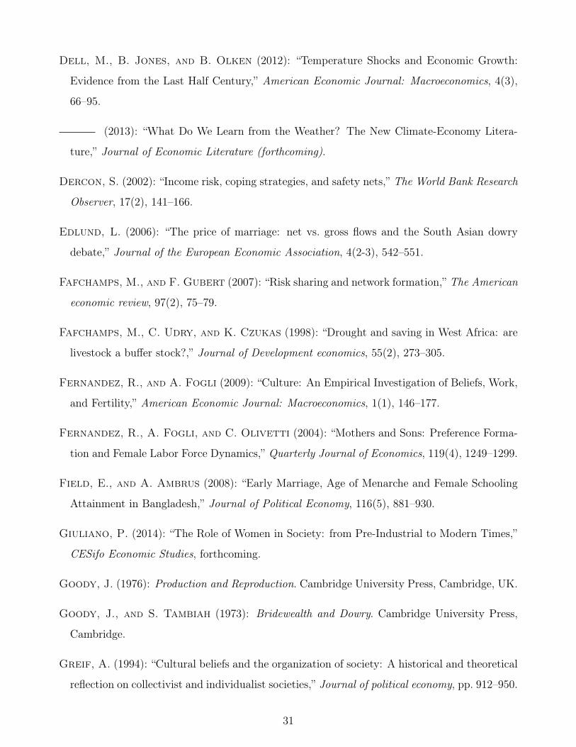
References

Alesina, A., Y. Algan, P. Cahuc, and P. Giuliano (2010): “Family Values and the

Regulation of Labor,” NBER Working Paper 15747.

Alesina, A., P. Giuliano, and N. Nunn (2013): “On the Origins of Gender Roles: Women

and the Plough,” Quarterly Journal of Economics, 128(2), 469–530.

Algan, Y., and P. Cahuc (2010): “Inherited Trust and Growth,” American Economic Review,

100(5), 2060–2092.

Anderson, S. (2003): “Why Dowry Payments Declined With Modernization in Europe but are

Rising in India,” Journal of Political Economy, 111(2), 269–310.

(2007): “The Economics of Dowry and Brideprice,” Journal of Economic Perspectives,

21(4), 151–174.

Anderson, S., and C. Bidner (2015): “Property Rights Over Marital Transfers,” Quarterly

Journal of Economics.

Angelucci, M., G. De Giorgi, M. A. Rangel, and I. Rasul (2010): “Family networks

and school enrolment: Evidence from a randomized social experiment,” Journal of public

Economics, 94(3), 197–221.

Arunachalam, R., and S. Naidu (2010): “The price of fertility: marriage markets and family

planning in Bangladesh,” .

Ashraf, N., N. Bau, N. Nunn, and A. Voena (2016): “Bride price and female education,”

Unpublished Manuscript.

Atkin, D. (2016): “The caloric costs of culture: Evidence from Indian migrants,” The American

Economic Review, 106(4), 1144–1181.

Bank, W. (2014): “Untying the Knot: Exploring Early Marriage in Fragile States,” .

29

Bau, N. (2016): “Can Policy Crowd Out Culture?,” working paper.

Becker, G. (1991): A Treatise on the Family. Enlarged edition, Cambridge, MA: Harvard

University Press.

Bloch, E., and V. Rao (2002): “Terror as a Bargaining Instrument: Dowry violence in rural

India,” American Economic Review, 92(4), 1029–1043.

Boserup, E. (1970): Woman’s Role in Economic Development. George Allen and Unwin Ltd.,

London.

Botticini, M. (1999): “A Loveless Economy? Intergenerational Altruism and the Marriage

Market in a Tuscan Town, 1415-1436,” The Journal of Economic History, 59, No. 1, 104–121.

Botticini, M., and A. Siow (2003): “Why Dowries?,” The American Economic Review, 93,

No. 4, 1385–1398.

Burke, M., E. Gong, and K. Jones (2014): “Income Shocks and HIV in Africa,” Economic

Journal (forthcoming).

Caldwell, J., P. Reddy, and P. Caldwell (1983): “The Causes of Marriage Change in

South India,” Population Studies, 37(3), 343–361.

Chowdhury, A. (2010): “Money and Marriage: The Practice of Dowry and Brideprice in Rural

India,” presented at the Population Association of America 2010 Annual Meeting: Dallas,

Texas.

Corno, L., and A. Voena (2016): “Selling daughters: age of marriage, income shocks and

bride price tradition,” Unpublished Manuscript.

Currie, J., and M. Neidell (2005): “Air Pollution and Infant Health: What Can We Learn

from California’s Recent Experience,” Quarterly Journal of Economics, 120(3), 1003–1030.

De Weerdt, J., and S. Dercon (2006): “Risk-sharing networks and insurance against illness,”

Journal of development Economics, 81(2), 337–356.

Decker, M., and H. Hoogeveen (2002): “Bridewealth and Household Security in Rural

Zimbabwe,” Journal of African Economies, 11(1), 114–145.

30

Dell, M., B. Jones, and B. Olken (2012): “Temperature Shocks and Economic Growth:

Evidence from the Last Half Century,” American Economic Journal: Macroeconomics, 4(3),

66–95.

(2013): “What Do We Learn from the Weather? The New Climate-Economy Litera-

ture,” Journal of Economic Literature (forthcoming).

Dercon, S. (2002): “Income risk, coping strategies, and safety nets,” The World Bank Research

Observer, 17(2), 141–166.

Edlund, L. (2006): “The price of marriage: net vs. gross flows and the South Asian dowry

debate,” Journal of the European Economic Association, 4(2-3), 542–551.

Fafchamps, M., and F. Gubert (2007): “Risk sharing and network formation,” The American

economic review, 97(2), 75–79.

Fafchamps, M., C. Udry, and K. Czukas (1998): “Drought and saving in West Africa: are

livestock a buffer stock?,” Journal of Development economics, 55(2), 273–305.

Fernandez, R., and A. Fogli (2009): “Culture: An Empirical Investigation of Beliefs, Work,

and Fertility,” American Economic Journal: Macroeconomics, 1(1), 146–177.

Fernandez, R., A. Fogli, and C. Olivetti (2004): “Mothers and Sons: Preference Forma-

tion and Female Labor Force Dynamics,” Quarterly Journal of Economics, 119(4), 1249–1299.

Field, E., and A. Ambrus (2008): “Early Marriage, Age of Menarche and Female Schooling

Attainment in Bangladesh,” Journal of Political Economy, 116(5), 881–930.

Giuliano, P. (2014): “The Role of Women in Society: from Pre-Industrial to Modern Times,”

CESifo Economic Studies, forthcoming.

Goody, J. (1976): Production and Reproduction. Cambridge University Press, Cambridge, UK.

Goody, J., and S. Tambiah (1973): Bridewealth and Dowry. Cambridge University Press,

Cambridge.

Greif, A. (1994): “Cultural beliefs and the organization of society: A historical and theoretical

reflection on collectivist and individualist societies,” Journal of political economy, pp. 912–950.

31

Jacoby, H. G. (1995): “The Economics of Polygyny in Sub-Saharan Africa: Female Produc-

tivity and the Demand for Wives in Côte d’Ivoire,” Journal of Political Economy, 103, No. 5,

938–971.

Jayachandran, S. (2006): “Selling Labor Low: Wage Responses to Productivity Shocks in

Developing Countries,” Journal of Political Economy, 114(3), 538–575.

Jensen, R., and R. Thornton (2003): “Early Female Marriage in the Developing World,”

Gender and Development, 11(2), 9–19.

La Ferrara, E. (2007): “Descent Rules and Strategic Transfers. Evidence from Matrilineal

Groups in Ghana,” Journal of Development Economics, 83 (2), 280–301.

La Ferrara, E., and A. Milazzo (2012): “Customary Norms, Inheritance and human capital:

evidence from a reform of the matrilineal system in Ghana,” working paper.

Mbaye, L., and N. Wagner (2013): “Bride Price and Fertility Decisions: Evidence from Rural

Senegal,” IZA Discussion Paper No. 770 (November).

Miguel, E., S. Satyanath, and E. Sergenti (2004): “Economic Shocks and Civil Conflict:

An Instrumental Variables Approach,” Journal of Political Economy, 112 (41)), 225–253.

Morten, M. (2016): “Temporary migration and endogenous risk sharing in village india,”

Discussion paper, National Bureau of Economic Research.

Murdock, G. P. (1967): Ethnographic Atlas. University of Pittsburgh Press, Pittsburgh.

Nunn, N., and L. Wantchekon (2011): “The slave trade and the origins of mistrust in

Africa,” The American Economic Review, 101(7), 3221–3252.

Pullum, T. W. (2006): “An Assessment of Age and Date Reporting in the DHS Surveys,

1985-2003,” DHS Methodological Reports, 5.

Rao, V. (1993): “The rising price of husbands: A hedonic analysis of dowry increases in rural

India,” Journal of Political Economy, pp. 666–677.

Rosenzweig, M. R., and O. Stark (1989): “Consumption smoothing, migration, and mar-

riage: Evidence from rural India,” The Journal of Political Economy, pp. 905–926.

32

Roy, S. (2015): “Empowering women? Inheritance rights, female education and dowry payments

in India,” Journal of Development Economics, 114, 233–251.

Sautmann, A. (2012): “Partner Search and Demographics: The Marriage Squeeze in India,”

Working Paper (July).

Schlenker, W., and D. Lobell (2010): “Robust Negative Impacts of Climate Change on

African Agriculture,” Environmental Research Letters, 5, 01410.

Sekhri, S., and A. Storeygard (2013): “Dowry Deaths: Consumption Smoothing in Re-

sponse to Climate Variability in India,” Working Paper (March).

Shah, M., and B. M. Steinberg (2016): “Drought of opportunities: contemporaneous and

long term impacts of rainfall shocks on human capital,” Journal of Political Economy.

Shleifer, A., and R. Vishny (1992): “Liquidation Values and Debt Capacity: A Market

Equilibrium,” The Journal of Finance, XLVII(4), 1343–1366.

Tabellini, G. (2010): “Culture and institutions: economic development in the regions of Eu-

rope,” Journal of the European Economic Association, 8(4), 677–716.

Tertilt, M. (2005): “Polygyny, fertility, and savings,” Journal of Political Economy, 113(6),

1341–1371.

Townsend, R. M. (1994): “Risk and insurance in village India,” Econometrica: Journal of the

Econometric Society, pp. 539–591.

Vogl, T. (2013): “Marriage Institutions and Sibling Competition: Evidence from South Asia,”

Quarterly Journal of Economics, 128(3), 1017–1072.

World Bank (2015): World Development Report 2015: Mind, Society, and Behavior. World

Bank Publications, Washington, D.C.

Worldvision (2013): “Voice and Agency: Empowering Women and Girls for Shared Prosper-

ity,” .

Figures and Tables

33

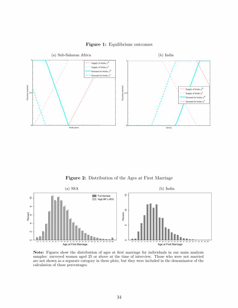
Figure 1: Equilibrium outcomes

(a) Sub-Saharan Africa

0

0.5

1

Frac

tion

mar

ried

bride price

Supply of brides yH

Supply of brides yL

Demand for brides yH

Demand for brides yL

(b) India

0

0.5

1

Frac

tion

mar

ried

dowry

Supply of brides yH

Supply of brides yL

Demand for brides yH

Demand for brides yL

Figure 2: Distribution of the Ages at First Marriage

(a) SSA

02

46

810

Per

cent

10 11 12 13 14 15 16 17 18 19 20 21 22 23 24 25 26 27 28 29 30 31 32 33 34 35+

Age at First MarriageNote: Figure shows the distribution of ages at first marriage for women aged 25+ at interview.

Distribution of Ages at Women's First Marriage: SSA

Full SampleHigh BP ≥ 80%

(b) India

05

1015

Per

cent

10 11 12 13 14 15 16 17 18 19 20 21 22 23 24 25 26 27 28 29 30 31 32 33 34 35+

Age at First MarriageNote: Figure shows the distribution of ages at first marriage for women aged 25+ at interview.

Distribution of Ages at Women's First Marriage: India

Note: Figures show the distribution of ages at first marriage for individuals in our main analysissamples: surveyed women aged 25 or above at the time of interview. Those who were not marriedare not shown as a separate category in these plots, but they were included in the denominator of thecalculation of these percentages.

34

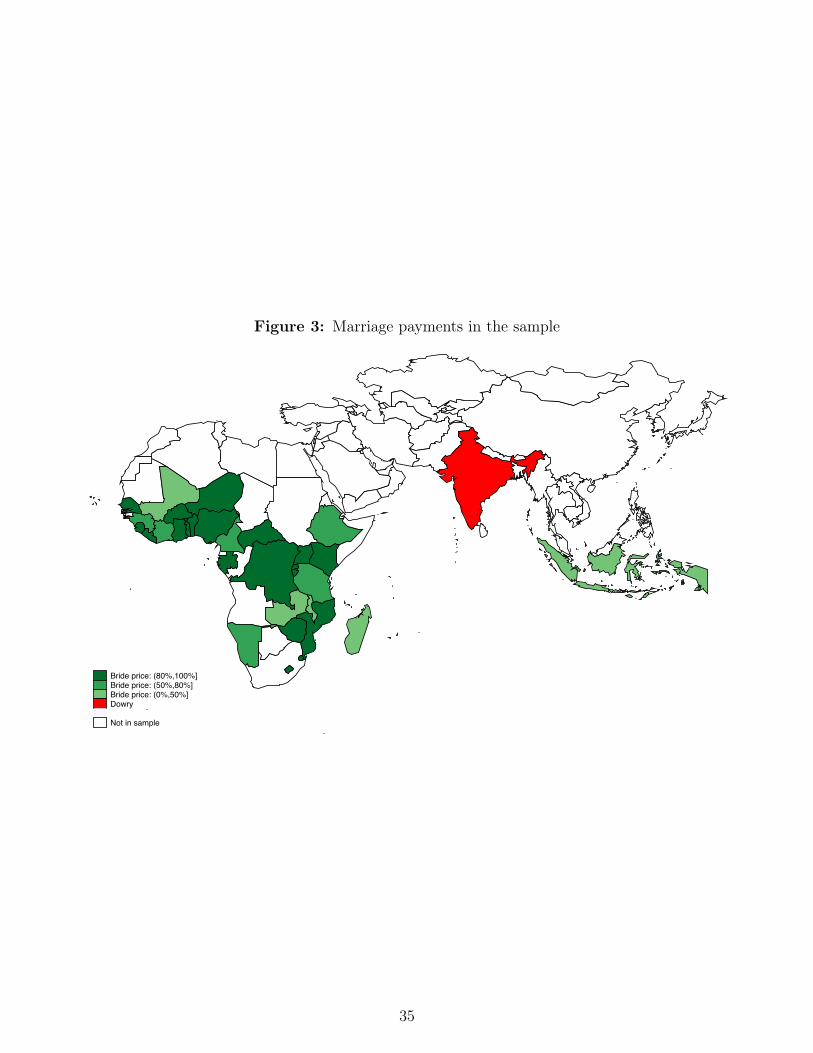
Figure 3: Marriage payments in the sample

Bride price: (80%,100%]Bride price: (50%,80%]Bride price: (0%,50%]Dowry

Not in sample

35

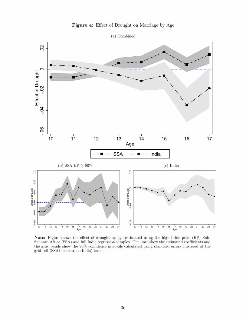
Figure 4: Effect of Drought on Marriage by Age

(a) Combined-.0

6-.0

4-.0

20

.02

Effe

ct o

f Dro

ught

10 11 12 13 14 15 16 17Age

SSA IndiaSSA: The number of observations is 2,447,982. The adjusted R-squared is 7.61%.India: The number of observations is 674,819. The adjusted R-squared is 10.13%.(b) SSA BP ≥ 80%

-0.0

2-0

.01

0.00

0.01

0.02

0.03

Effe

ct o

f Dro

ught

10 11 12 13 14 15 16 17 18 19 20 21 22 23 24Age

The number of observations is 2,248,576. The adjusted R-squared is 7.32%.

(c) India

-0.1

0-0

.05

0.00

0.05

Effe

ct o

f Dro

ught

10 11 12 13 14 15 16 17 18 19 20 21 22 23 24Age

The number of observations is 838,846. The adjusted R-squared is 11.51%.

Note: Figure shows the effect of drought by age estimated using the high bride price (BP) Sub-Saharan Africa (SSA) and full India regression samples. The lines show the estimated coefficients andthe gray bands show the 95% confidence intervals calculated using standard errors clustered at thegrid cell (SSA) or district (India) level.

36

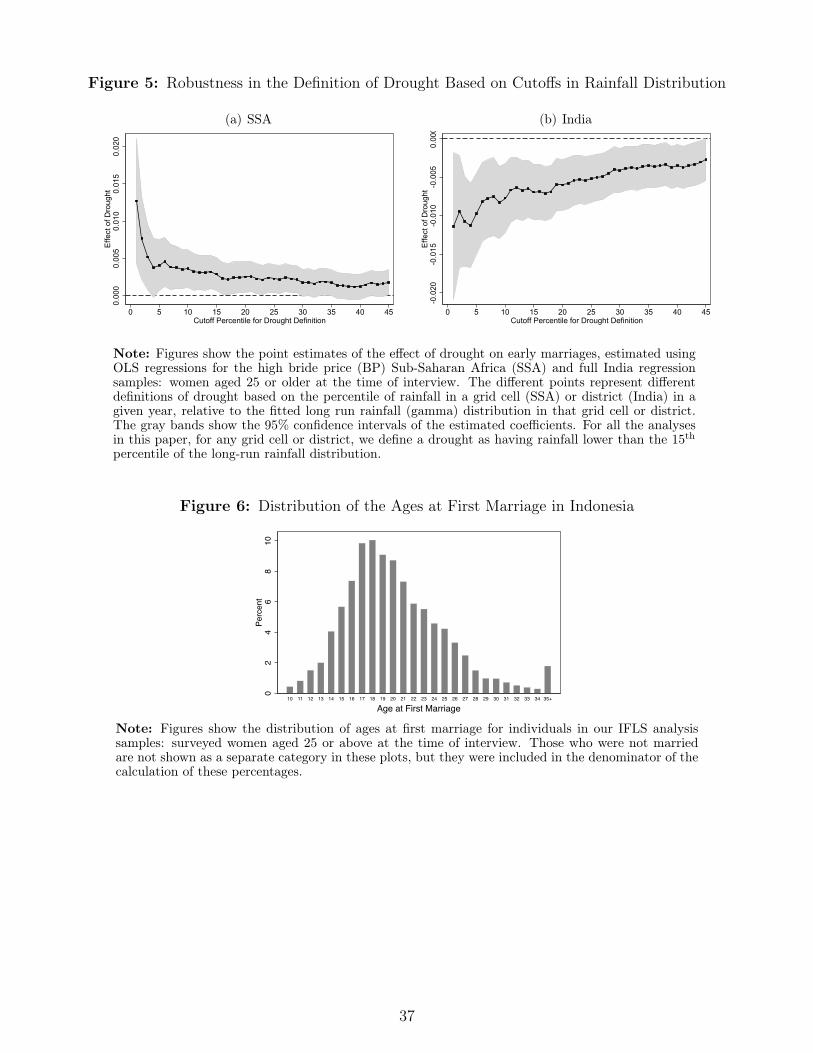
Figure 5: Robustness in the Definition of Drought Based on Cutoffs in Rainfall Distribution

(a) SSA0.

000

0.00

50.

010

0.01

50.

020

Effe

ct o

f Dro

ught

0 5 10 15 20 25 30 35 40 45Cutoff Percentile for Drought Definition

Robustness to Rainfall Cutoff: SSA, BP ≥ 80% (b) India

-0.0

20-0

.015

-0.0

10-0

.005

0.00

0E

ffect

of D

roug

ht

0 5 10 15 20 25 30 35 40 45Cutoff Percentile for Drought Definition

Robustness to Rainfall Cutoff: India

Note: Figures show the point estimates of the effect of drought on early marriages, estimated usingOLS regressions for the high bride price (BP) Sub-Saharan Africa (SSA) and full India regressionsamples: women aged 25 or older at the time of interview. The different points represent differentdefinitions of drought based on the percentile of rainfall in a grid cell (SSA) or district (India) in agiven year, relative to the fitted long run rainfall (gamma) distribution in that grid cell or district.The gray bands show the 95% confidence intervals of the estimated coefficients. For all the analysesin this paper, for any grid cell or district, we define a drought as having rainfall lower than the 15th

percentile of the long-run rainfall distribution.

Figure 6: Distribution of the Ages at First Marriage in Indonesia

02

46

810

Perc

ent

10 11 12 13 14 15 16 17 18 19 20 21 22 23 24 25 26 27 28 29 30 31 32 33 34 35+

Age at First MarriageNote: Figure shows the distribution of ages at first marriage for women aged 25+ at interview.

Distribution of Ages at Women's First Marriage: Indonesia

Note: Figures show the distribution of ages at first marriage for individuals in our IFLS analysissamples: surveyed women aged 25 or above at the time of interview. Those who were not marriedare not shown as a separate category in these plots, but they were included in the denominator of thecalculation of these percentages.

37

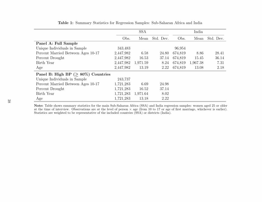
Table 1: Summary Statistics for Regression Samples: Sub-Saharan Africa and India

SSA India

Obs. Mean Std. Dev. Obs. Mean Std. Dev.Panel A: Full SampleUnique Individuals in Sample 343,483 96,954Percent Married Between Ages 10-17 2,447,982 6.58 24.80 674,819 8.86 28.41Percent Drought 2,447,982 16.53 37.14 674,819 15.45 36.14Birth Year 2,447,982 1,971.59 8.24 674,819 1,967.38 7.31Age 2,447,982 13.19 2.22 674,819 13.08 2.18

Panel B: High BP (≥ 80%) CountriesUnique Individuals in Sample 243,737Percent Married Between Ages 10-17 1,721,283 6.69 24.98Percent Drought 1,721,283 16.52 37.14Birth Year 1,721,283 1,971.64 8.02Age 1,721,283 13.18 2.22

Note: Table shows summary statistics for the main Sub-Saharan Africa (SSA) and India regression samples: women aged 25 or olderat the time of interview. Observations are at the level of person × age (from 10 to 17 or age of first marriage, whichever is earlier).Statistics are weighted to be representative of the included countries (SSA) or districts (India).

38

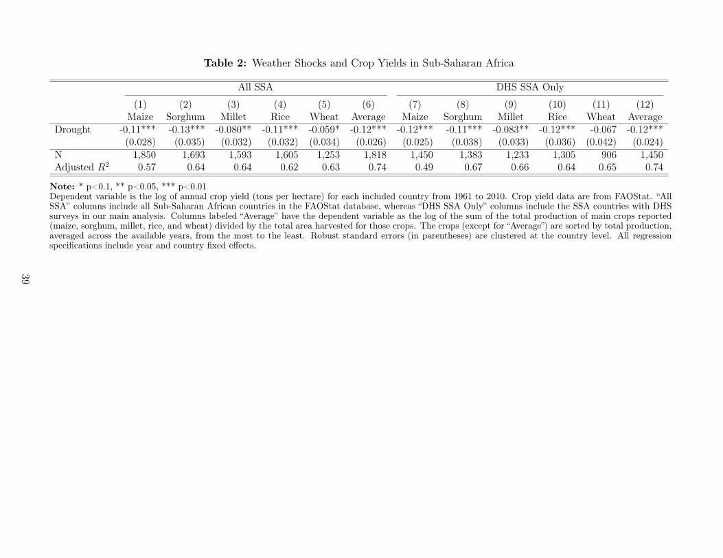
Table 2: Weather Shocks and Crop Yields in Sub-Saharan Africa

All SSA DHS SSA Only

(1) (2) (3) (4) (5) (6) (7) (8) (9) (10) (11) (12)Maize Sorghum Millet Rice Wheat Average Maize Sorghum Millet Rice Wheat Average

Drought -0.11*** -0.13*** -0.080** -0.11*** -0.059* -0.12*** -0.12*** -0.11*** -0.083** -0.12*** -0.067 -0.12***(0.028) (0.035) (0.032) (0.032) (0.034) (0.026) (0.025) (0.038) (0.033) (0.036) (0.042) (0.024)

N 1,850 1,693 1,593 1,605 1,253 1,818 1,450 1,383 1,233 1,305 906 1,450Adjusted R2 0.57 0.64 0.64 0.62 0.63 0.74 0.49 0.67 0.66 0.64 0.65 0.74

Note: * p<0.1, ** p<0.05, *** p<0.01Dependent variable is the log of annual crop yield (tons per hectare) for each included country from 1961 to 2010. Crop yield data are from FAOStat. “AllSSA” columns include all Sub-Saharan African countries in the FAOStat database, whereas “DHS SSA Only” columns include the SSA countries with DHSsurveys in our main analysis. Columns labeled “Average” have the dependent variable as the log of the sum of the total production of main crops reported(maize, sorghum, millet, rice, and wheat) divided by the total area harvested for those crops. The crops (except for “Average”) are sorted by total production,averaged across the available years, from the most to the least. Robust standard errors (in parentheses) are clustered at the country level. All regressionspecifications include year and country fixed effects.

39

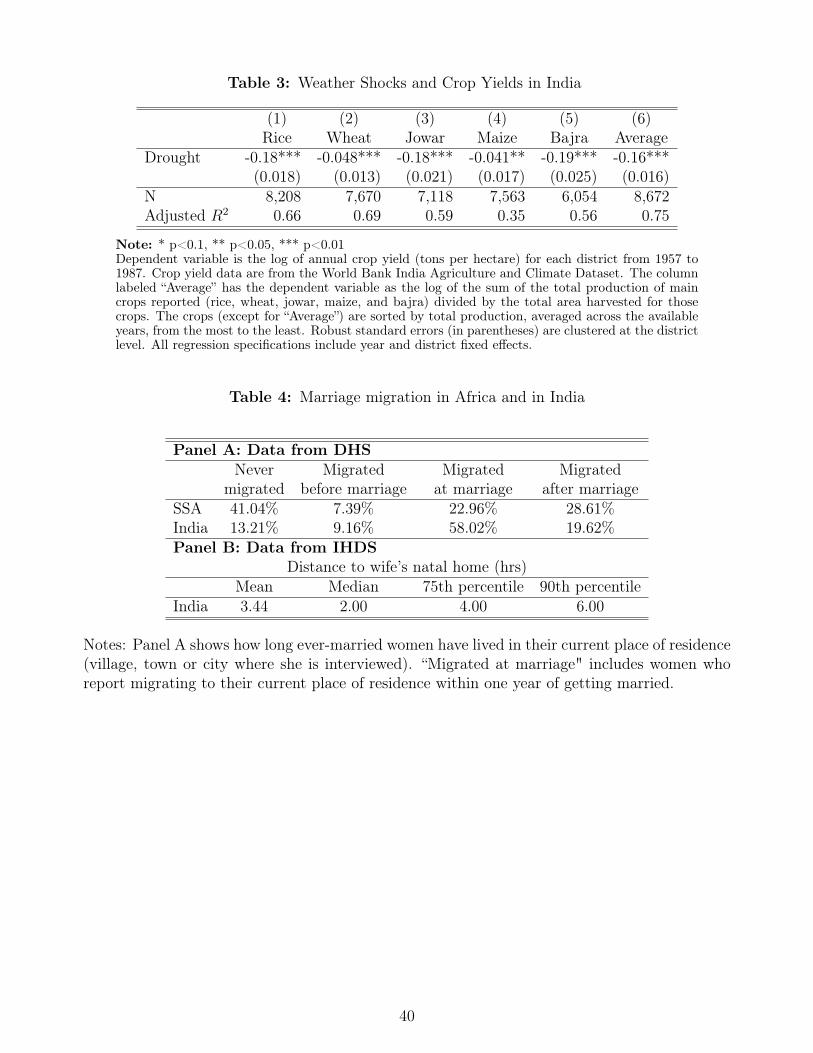
Table 3: Weather Shocks and Crop Yields in India

(1) (2) (3) (4) (5) (6)Rice Wheat Jowar Maize Bajra Average

Drought -0.18*** -0.048*** -0.18*** -0.041** -0.19*** -0.16***(0.018) (0.013) (0.021) (0.017) (0.025) (0.016)

N 8,208 7,670 7,118 7,563 6,054 8,672Adjusted R2 0.66 0.69 0.59 0.35 0.56 0.75

Note: * p<0.1, ** p<0.05, *** p<0.01Dependent variable is the log of annual crop yield (tons per hectare) for each district from 1957 to1987. Crop yield data are from the World Bank India Agriculture and Climate Dataset. The columnlabeled “Average” has the dependent variable as the log of the sum of the total production of maincrops reported (rice, wheat, jowar, maize, and bajra) divided by the total area harvested for thosecrops. The crops (except for “Average”) are sorted by total production, averaged across the availableyears, from the most to the least. Robust standard errors (in parentheses) are clustered at the districtlevel. All regression specifications include year and district fixed effects.

Table 4: Marriage migration in Africa and in India

Panel A: Data from DHSNever Migrated Migrated Migrated

migrated before marriage at marriage after marriageSSA 41.04% 7.39% 22.96% 28.61%India 13.21% 9.16% 58.02% 19.62%Panel B: Data from IHDS

Distance to wife’s natal home (hrs)Mean Median 75th percentile 90th percentile

India 3.44 2.00 4.00 6.00

Notes: Panel A shows how long ever-married women have lived in their current place of residence(village, town or city where she is interviewed). “Migrated at marriage" includes women whoreport migrating to their current place of residence within one year of getting married.

40

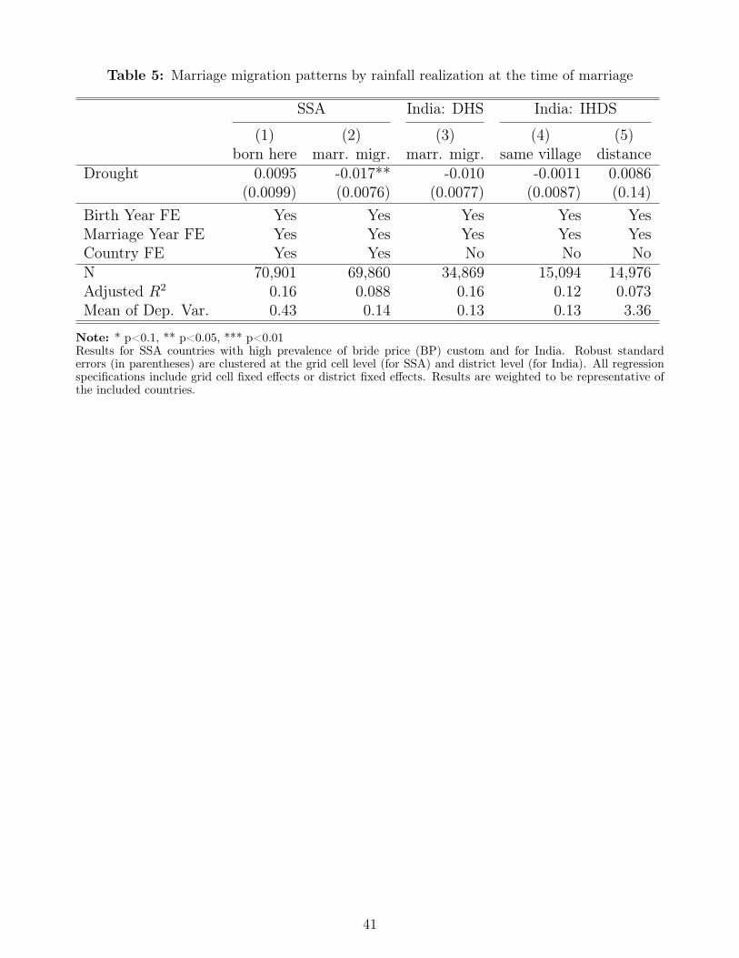
Table 5: Marriage migration patterns by rainfall realization at the time of marriage

SSA India: DHS India: IHDS

(1) (2) (3) (4) (5)born here marr. migr. marr. migr. same village distance

Drought 0.0095 -0.017** -0.010 -0.0011 0.0086(0.0099) (0.0076) (0.0077) (0.0087) (0.14)

Birth Year FE Yes Yes Yes Yes YesMarriage Year FE Yes Yes Yes Yes YesCountry FE Yes Yes No No NoN 70,901 69,860 34,869 15,094 14,976Adjusted R2 0.16 0.088 0.16 0.12 0.073Mean of Dep. Var. 0.43 0.14 0.13 0.13 3.36

Note: * p<0.1, ** p<0.05, *** p<0.01Results for SSA countries with high prevalence of bride price (BP) custom and for India. Robust standarderrors (in parentheses) are clustered at the grid cell level (for SSA) and district level (for India). All regressionspecifications include grid cell fixed effects or district fixed effects. Results are weighted to be representative ofthe included countries.

41

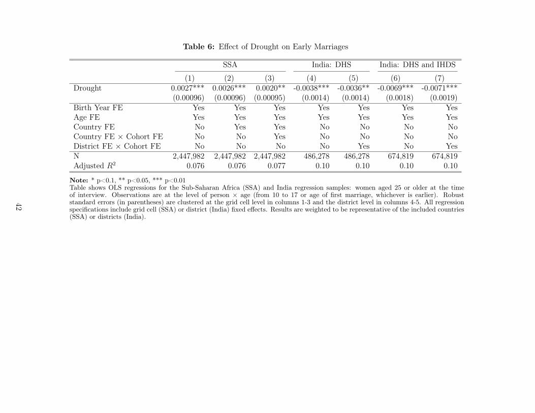
Table 6: Effect of Drought on Early Marriages

SSA India: DHS India: DHS and IHDS

(1) (2) (3) (4) (5) (6) (7)Drought 0.0027*** 0.0026*** 0.0020** -0.0038*** -0.0036** -0.0069*** -0.0071***

(0.00096) (0.00096) (0.00095) (0.0014) (0.0014) (0.0018) (0.0019)Birth Year FE Yes Yes Yes Yes Yes Yes YesAge FE Yes Yes Yes Yes Yes Yes YesCountry FE No Yes Yes No No No NoCountry FE × Cohort FE No No Yes No No No NoDistrict FE × Cohort FE No No No No Yes No YesN 2,447,982 2,447,982 2,447,982 486,278 486,278 674,819 674,819Adjusted R2 0.076 0.076 0.077 0.10 0.10 0.10 0.10

Note: * p<0.1, ** p<0.05, *** p<0.01Table shows OLS regressions for the Sub-Saharan Africa (SSA) and India regression samples: women aged 25 or older at the timeof interview. Observations are at the level of person × age (from 10 to 17 or age of first marriage, whichever is earlier). Robuststandard errors (in parentheses) are clustered at the grid cell level in columns 1-3 and the district level in columns 4-5. All regressionspecifications include grid cell (SSA) or district (India) fixed effects. Results are weighted to be representative of the included countries(SSA) or districts (India).

42

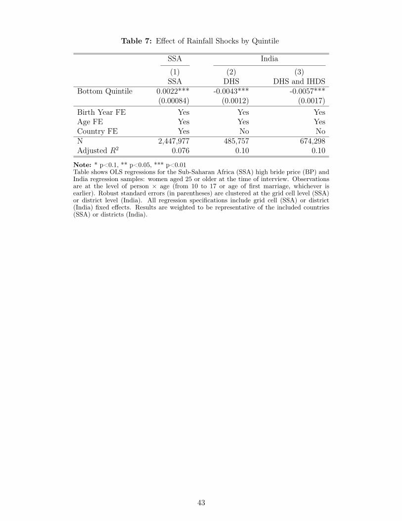
Table 7: Effect of Rainfall Shocks by Quintile

SSA India

(1) (2) (3)SSA DHS DHS and IHDS

Bottom Quintile 0.0022*** -0.0043*** -0.0057***(0.00084) (0.0012) (0.0017)

Birth Year FE Yes Yes YesAge FE Yes Yes YesCountry FE Yes No NoN 2,447,977 485,757 674,298Adjusted R2 0.076 0.10 0.10

Note: * p<0.1, ** p<0.05, *** p<0.01Table shows OLS regressions for the Sub-Saharan Africa (SSA) high bride price (BP) andIndia regression samples: women aged 25 or older at the time of interview. Observationsare at the level of person × age (from 10 to 17 or age of first marriage, whichever isearlier). Robust standard errors (in parentheses) are clustered at the grid cell level (SSA)or district level (India). All regression specifications include grid cell (SSA) or district(India) fixed effects. Results are weighted to be representative of the included countries(SSA) or districts (India).

43

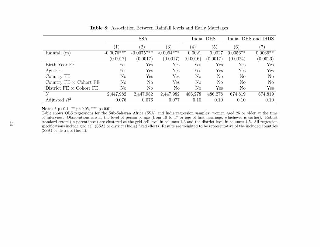
Table 8: Association Between Rainfall levels and Early Marriages

SSA India: DHS India: DHS and IHDS

(1) (2) (3) (4) (5) (6) (7)Rainfall (m) -0.0076*** -0.0075*** -0.0064*** 0.0021 0.0027 0.0056** 0.0066**

(0.0017) (0.0017) (0.0017) (0.0016) (0.0017) (0.0024) (0.0026)Birth Year FE Yes Yes Yes Yes Yes Yes YesAge FE Yes Yes Yes Yes Yes Yes YesCountry FE No Yes Yes No No No NoCountry FE × Cohort FE No No Yes No No No NoDistrict FE × Cohort FE No No No No Yes No YesN 2,447,982 2,447,982 2,447,982 486,278 486,278 674,819 674,819Adjusted R2 0.076 0.076 0.077 0.10 0.10 0.10 0.10

Note: * p<0.1, ** p<0.05, *** p<0.01Table shows OLS regressions for the Sub-Saharan Africa (SSA) and India regression samples: women aged 25 or older at the timeof interview. Observations are at the level of person × age (from 10 to 17 or age of first marriage, whichever is earlier). Robuststandard errors (in parentheses) are clustered at the grid cell level in columns 1-3 and the district level in columns 4-5. All regressionspecifications include grid cell (SSA) or district (India) fixed effects. Results are weighted to be representative of the included countries(SSA) or districts (India).

44

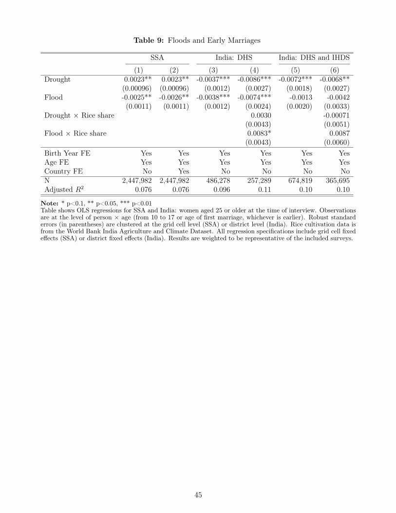
Table 9: Floods and Early Marriages

SSA India: DHS India: DHS and IHDS

(1) (2) (3) (4) (5) (6)Drought 0.0023** 0.0023** -0.0037*** -0.0086*** -0.0072*** -0.0068**

(0.00096) (0.00096) (0.0012) (0.0027) (0.0018) (0.0027)Flood -0.0025** -0.0026** -0.0038*** -0.0074*** -0.0013 -0.0042

(0.0011) (0.0011) (0.0012) (0.0024) (0.0020) (0.0033)Drought × Rice share 0.0030 -0.00071

(0.0043) (0.0051)Flood × Rice share 0.0083* 0.0087

(0.0043) (0.0060)Birth Year FE Yes Yes Yes Yes Yes YesAge FE Yes Yes Yes Yes Yes YesCountry FE No Yes No No No NoN 2,447,982 2,447,982 486,278 257,289 674,819 365,695Adjusted R2 0.076 0.076 0.096 0.11 0.10 0.10

Note: * p<0.1, ** p<0.05, *** p<0.01Table shows OLS regressions for SSA and India: women aged 25 or older at the time of interview. Observationsare at the level of person × age (from 10 to 17 or age of first marriage, whichever is earlier). Robust standarderrors (in parentheses) are clustered at the grid cell level (SSA) or district level (India). Rice cultivation data isfrom the World Bank India Agriculture and Climate Dataset. All regression specifications include grid cell fixedeffects (SSA) or district fixed effects (India). Results are weighted to be representative of the included surveys.

45

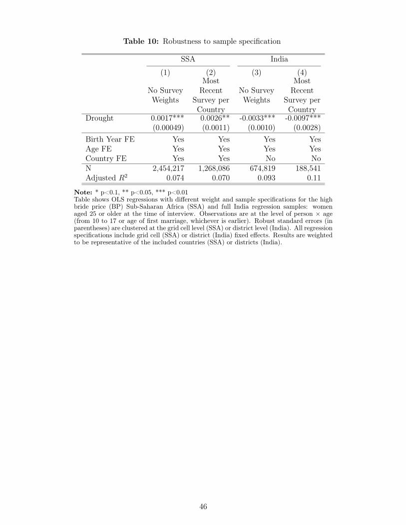
Table 10: Robustness to sample specification

SSA India

(1) (2) (3) (4)

No SurveyWeights

MostRecent

Survey perCountry

No SurveyWeights

MostRecent

Survey perCountry

Drought 0.0017*** 0.0026** -0.0033*** -0.0097***(0.00049) (0.0011) (0.0010) (0.0028)

Birth Year FE Yes Yes Yes YesAge FE Yes Yes Yes YesCountry FE Yes Yes No NoN 2,454,217 1,268,086 674,819 188,541Adjusted R2 0.074 0.070 0.093 0.11

Note: * p<0.1, ** p<0.05, *** p<0.01Table shows OLS regressions with different weight and sample specifications for the highbride price (BP) Sub-Saharan Africa (SSA) and full India regression samples: womenaged 25 or older at the time of interview. Observations are at the level of person × age(from 10 to 17 or age of first marriage, whichever is earlier). Robust standard errors (inparentheses) are clustered at the grid cell level (SSA) or district level (India). All regressionspecifications include grid cell (SSA) or district (India) fixed effects. Results are weightedto be representative of the included countries (SSA) or districts (India).

46

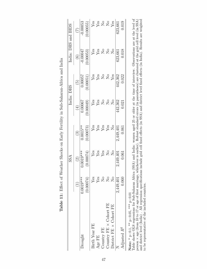
Tab

le11

:Effe

ctof

Weather

Shocks

onEarly

Fertility

inSu

b-Sa

haran-Africaan

dIndia

SSA

India:

DHS

India:

DHSan

dIH

DS

(1)

(2)

(3)

(4)

(5)

(6)

(7)

Droug

ht0.00

19**

*0.00

19**

*0.00

15**

0.0006

70.00

057

-0.000

47-0.000

53(0.000

74)

(0.000

74)

(0.000

73)

(0.000

49)

(0.000

51)

(0.000

53)

(0.000

55)

Birth

YearFE

Yes

Yes

Yes

Yes

Yes

Yes

Yes

Age

FE

Yes

Yes

Yes

Yes

Yes

Yes

Yes

Cou

ntry

FE

No

Yes

Yes

No

No

No

No

Cou

ntry

FE×

Coh

ortFE

No

No

Yes

No

No

No

No

DistrictFE×

Coh

ortFE

No

No

No

No

Yes

No

Yes

N2,44

9,40

12,44

9,40

12,44

9,40

144

2,362

442,36

262

3,66

162

3,66

1AdjustedR

20.06

00.06

10.06

10.02

10.02

20.01

80.01

9

Not

e:*p<

0.1,

**p<

0.05,*

**p<

0.01

Tab

leshow

sOLS

regression

sforSu

b-Sa

haranAfrica(SSA

)an

dIndia:

wom

enaged

25or

olderat

thetimeof

interview.Observation

sareat

thelevelof

person×

age(from

10to

17or

ageof

first

marriage,

whichever

isearlier).Rob

uststan

dard

errors

(inpa

rentheses)

areclusteredat

thegrid

celllevel(in

SSA)

anddistrict

level(

India)

.Allregression

specification

sinclud

egrid

cellfix

edeff

ects

(inSS

A)an

ddistrict

levelfi

xedeff

ects

(inIndia).Results

areweigh

ted

tobe

representative

oftheinclud

edcoun

tries.

47

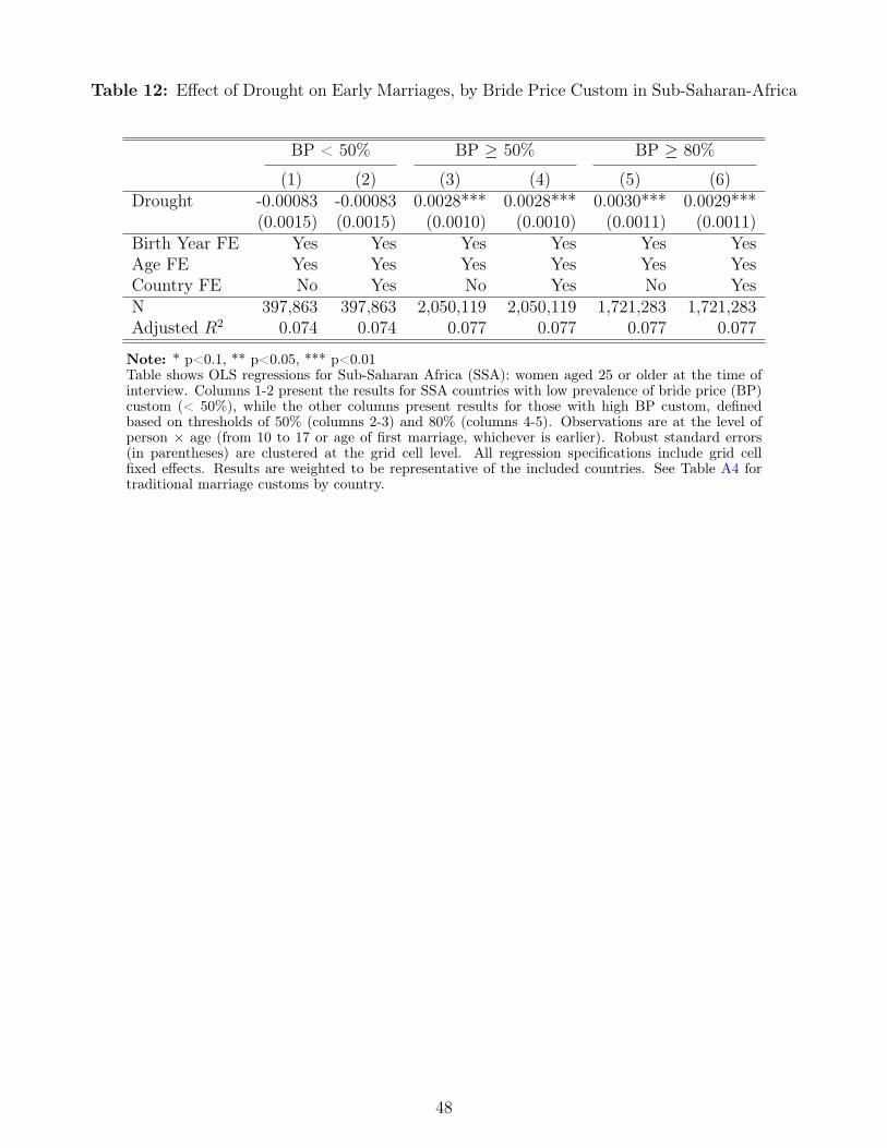
Table 12: Effect of Drought on Early Marriages, by Bride Price Custom in Sub-Saharan-Africa

BP < 50% BP ≥ 50% BP ≥ 80%

(1) (2) (3) (4) (5) (6)Drought -0.00083 -0.00083 0.0028*** 0.0028*** 0.0030*** 0.0029***

(0.0015) (0.0015) (0.0010) (0.0010) (0.0011) (0.0011)Birth Year FE Yes Yes Yes Yes Yes YesAge FE Yes Yes Yes Yes Yes YesCountry FE No Yes No Yes No YesN 397,863 397,863 2,050,119 2,050,119 1,721,283 1,721,283Adjusted R2 0.074 0.074 0.077 0.077 0.077 0.077

Note: * p<0.1, ** p<0.05, *** p<0.01Table shows OLS regressions for Sub-Saharan Africa (SSA): women aged 25 or older at the time ofinterview. Columns 1-2 present the results for SSA countries with low prevalence of bride price (BP)custom (< 50%), while the other columns present results for those with high BP custom, definedbased on thresholds of 50% (columns 2-3) and 80% (columns 4-5). Observations are at the level ofperson × age (from 10 to 17 or age of first marriage, whichever is earlier). Robust standard errors(in parentheses) are clustered at the grid cell level. All regression specifications include grid cellfixed effects. Results are weighted to be representative of the included countries. See Table A4 fortraditional marriage customs by country.

48

Table 13: Effect of Drought on Early Marriages, by Religion in India

DHS DHS and IHDS

(1) (2) (3) (4)Drought × Hindu -0.0043*** -0.0039** -0.0081*** -0.0083***

(0.0015) (0.0016) (0.0022) (0.0022)Drought × Not hindu -0.0017 -0.0024 -0.0031 -0.0027

(0.0023) (0.0023) (0.0034) (0.0034)Birth Year FE × Hindu FE Yes Yes Yes YesAge FE × Hindu FE Yes Yes Yes YesDistrict FE × Cohort FE No Yes No YesN 462,112 462,112 650,653 650,653Adjusted R2 0.10 0.10 0.10 0.11

Note: * p<0.1, ** p<0.05, *** p<0.01Table shows OLS regressions for India: women aged 25 or older at the time of interview. Observationsare at the level of person × age (from 10 to 17 or age of first marriage, whichever is earlier). Robuststandard errors (in parentheses) are clustered at the district level. All regression specifications includedistrict fixed effects. Results in columns 3 and 4 are weighted to be representative of the includedsurveys.

49

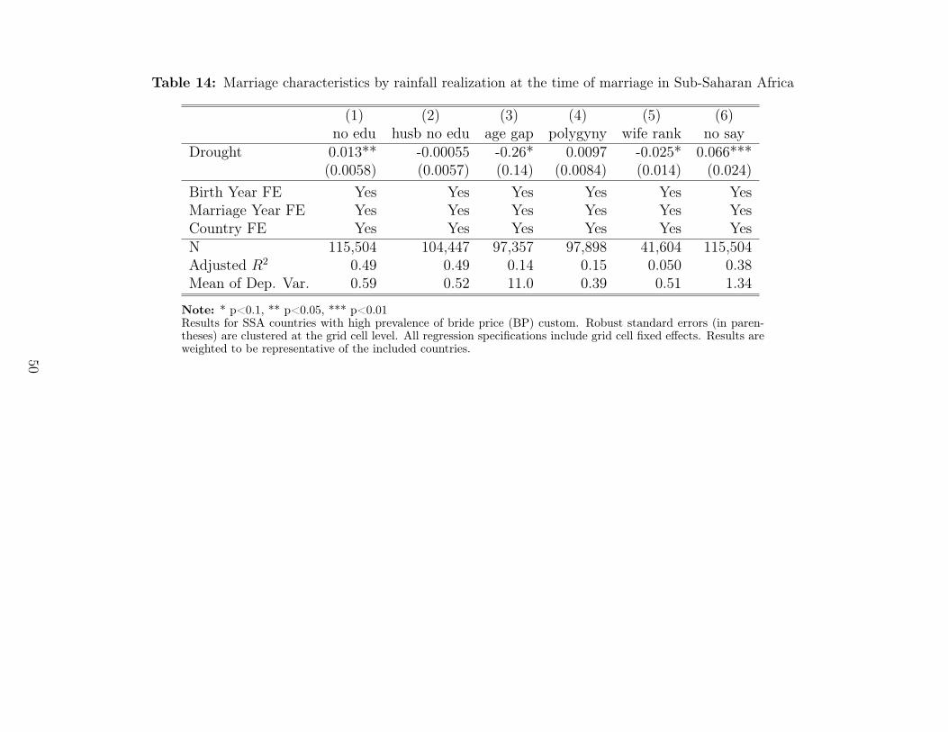
Table 14: Marriage characteristics by rainfall realization at the time of marriage in Sub-Saharan Africa

(1) (2) (3) (4) (5) (6)no edu husb no edu age gap polygyny wife rank no say

Drought 0.013** -0.00055 -0.26* 0.0097 -0.025* 0.066***(0.0058) (0.0057) (0.14) (0.0084) (0.014) (0.024)

Birth Year FE Yes Yes Yes Yes Yes YesMarriage Year FE Yes Yes Yes Yes Yes YesCountry FE Yes Yes Yes Yes Yes YesN 115,504 104,447 97,357 97,898 41,604 115,504Adjusted R2 0.49 0.49 0.14 0.15 0.050 0.38Mean of Dep. Var. 0.59 0.52 11.0 0.39 0.51 1.34

Note: * p<0.1, ** p<0.05, *** p<0.01Results for SSA countries with high prevalence of bride price (BP) custom. Robust standard errors (in paren-theses) are clustered at the grid cell level. All regression specifications include grid cell fixed effects. Results areweighted to be representative of the included countries.50

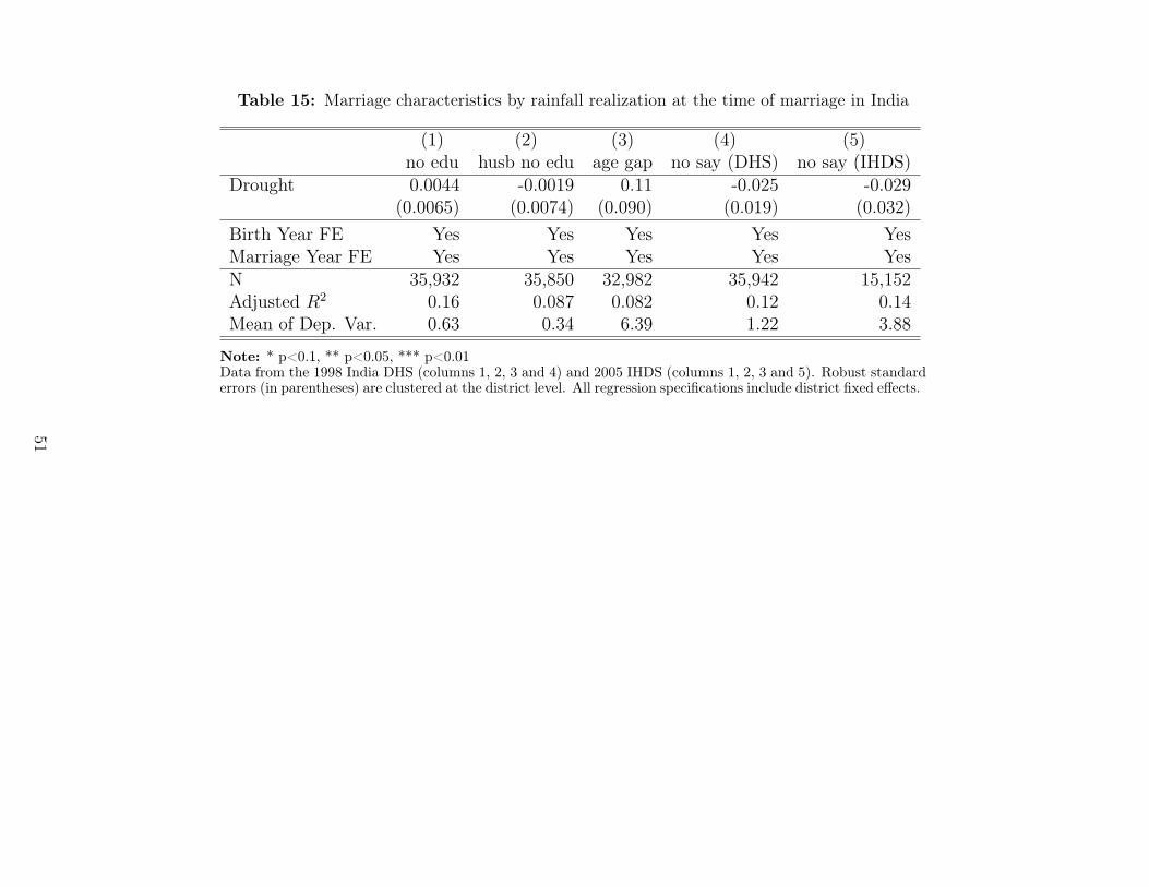
Table 15: Marriage characteristics by rainfall realization at the time of marriage in India

(1) (2) (3) (4) (5)no edu husb no edu age gap no say (DHS) no say (IHDS)

Drought 0.0044 -0.0019 0.11 -0.025 -0.029(0.0065) (0.0074) (0.090) (0.019) (0.032)

Birth Year FE Yes Yes Yes Yes YesMarriage Year FE Yes Yes Yes Yes YesN 35,932 35,850 32,982 35,942 15,152Adjusted R2 0.16 0.087 0.082 0.12 0.14Mean of Dep. Var. 0.63 0.34 6.39 1.22 3.88

Note: * p<0.1, ** p<0.05, *** p<0.01Data from the 1998 India DHS (columns 1, 2, 3 and 4) and 2005 IHDS (columns 1, 2, 3 and 5). Robust standarderrors (in parentheses) are clustered at the district level. All regression specifications include district fixed effects.

51

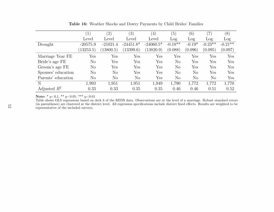
Table 16: Weather Shocks and Dowry Payments by Child Brides’ Families

(1) (2) (3) (4) (5) (6) (7) (8)Level Level Level Level Log Log Log Log

Drought -20575.9 -21021.4 -24451.8* -24060.5* -0.18** -0.19* -0.23** -0.21**(13253.5) (13800.5) (13399.6) (13820.9) (0.088) (0.096) (0.095) (0.097)

Marriage Year FE Yes Yes Yes Yes Yes Yes Yes YesBride’s age FE No Yes Yes Yes No Yes Yes YesGroom’s age FE No Yes Yes Yes No Yes Yes YesSpouses’ education No No Yes Yes No No Yes YesParents’ education No No No Yes No No No YesN 1,993 1,951 1,951 1,949 1,790 1,772 1,772 1,770Adjusted R2 0.33 0.33 0.35 0.35 0.46 0.46 0.51 0.52

Note: * p<0.1, ** p<0.05, *** p<0.01Table shows OLS regressions based on deck 8 of the REDS data. Observations are at the level of a marriage. Robust standard errors(in parentheses) are clustered at the district level. All regression specifications include district fixed effects. Results are weighted to berepresentative of the included surveys.

52

Table 17: Summary Statistics for Regression Samples: Indonesia

Obs. Mean Std. Dev. Obs. Mean Std. Dev.Panel A: Full SampleUnique Individuals in Sample 7,532Percent Married Between Ages 10-17 56,295 4.19 20.05Percent Drought 56,295 17.01 37.57Birth Year 56,295 1,966.72 8.55Age 56,295 13.34 2.26

Panel B: Sample According to Ethnographic AtlasBride Price Groups No Bride Price Groups

Unique Individuals in Sample 1,622 5,516Percent Married Between Ages 10-17 12,109 4.10 19.82 41,202 4.25 20.17Percent Drought 12,109 24.56 43.05 41,202 14.41 35.12Birth Year 12,109 1,966.75 8.67 41,202 1,966.74 8.52Age 12,109 13.34 2.26 41,202 13.33 2.25

Note: Table shows summary statistics for the Indonesia regression samples: women aged 25 or older at the time of interview.Observations are at the level of person × age (from 10 to 17 or age of first marriage, whichever is earlier).

53

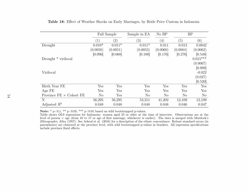
Table 18: Effect of Weather Shocks on Early Marriages, by Bride Price Custom in Indonesia

Full Sample Sample in EA No BP BP

(1) (2) (3) (4) (5) (6)Drought 0.010* 0.011* 0.011* 0.011 0.013 0.0042

(0.0050) (0.0051) (0.0053) (0.0060) (0.0084) (0.0062)[0.096] [0.068] [0.100] [0.176] [0.276] [0.548]

Drought * virilocal 0.015***(0.0067)[0.008]

Virilocal -0.022(0.027)[0.520]

Birth Year FE Yes Yes Yes Yes Yes YesAge FE Yes Yes Yes Yes Yes YesProvince FE × Cohort FE No Yes No No No NoN 56,295 56,295 53,311 41,202 12,109 12,109Adjusted R2 0.048 0.048 0.048 0.048 0.046 0.047

Note: * p<0.1, ** p<0.05, *** p<0.01 based on wild bootstrapped p-values.Table shows OLS regressions for Indonesia: women aged 25 or older at the time of interview. Observations are at thelevel of person × age (from 10 to 17 or age of first marriage, whichever is earlier). The data is merged with Murdock’sEthnographic Atlas (1957). See Ashraf et al. (2016) for a description of the ethnic concordance. Robust standard errors (inparentheses) are clustered at the province level, with wild bootstrapped p-values in brackets. All regression specificationsinclude province fixed effects.

54

A Appendix Tables and Figures

Table A1: List of Data Sets and Sources

Region/ Country Data Topic Source Year

Marriage Demographic and Health Survey (DHS) 1994-2014Sub-Saharan Africa Crop Yield FAOStat database 1960-2010

Conflict UCDP/PRIO Armed Conflict Dataset 1946-2015

Marriage Demographic and Health Survey (DHS) 1998-1999Marriage India Human Development Survey (IHDS) 2005

India Dowry Rural Economic and Demographic Survey (REDS) 1998GPS GADM database of Global Administrative AreasCrop Yield World Bank India Agriculture and Climate Data Set 1957-1987

Indonesia Marriage Indonesia Family Life Survey (IFLS) 2000-2007

Weather University of Delaware (UDel) 1900-2010Population World Development Indicators (WDI) 1990-2012Crop Calendar Maps Crop Calendar Dataset

(University of Wisconsin-Madison)

55

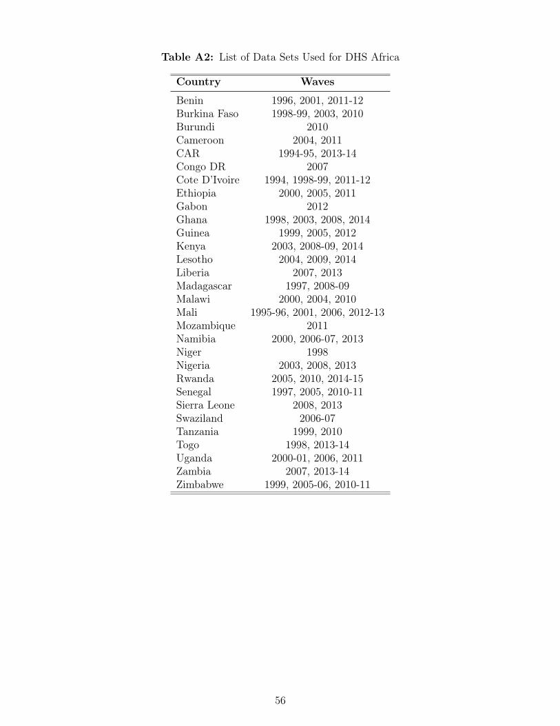
Table A2: List of Data Sets Used for DHS Africa

Country Waves

Benin 1996, 2001, 2011-12Burkina Faso 1998-99, 2003, 2010Burundi 2010Cameroon 2004, 2011CAR 1994-95, 2013-14Congo DR 2007Cote D’Ivoire 1994, 1998-99, 2011-12Ethiopia 2000, 2005, 2011Gabon 2012Ghana 1998, 2003, 2008, 2014Guinea 1999, 2005, 2012Kenya 2003, 2008-09, 2014Lesotho 2004, 2009, 2014Liberia 2007, 2013Madagascar 1997, 2008-09Malawi 2000, 2004, 2010Mali 1995-96, 2001, 2006, 2012-13Mozambique 2011Namibia 2000, 2006-07, 2013Niger 1998Nigeria 2003, 2008, 2013Rwanda 2005, 2010, 2014-15Senegal 1997, 2005, 2010-11Sierra Leone 2008, 2013Swaziland 2006-07Tanzania 1999, 2010Togo 1998, 2013-14Uganda 2000-01, 2006, 2011Zambia 2007, 2013-14Zimbabwe 1999, 2005-06, 2010-11

56

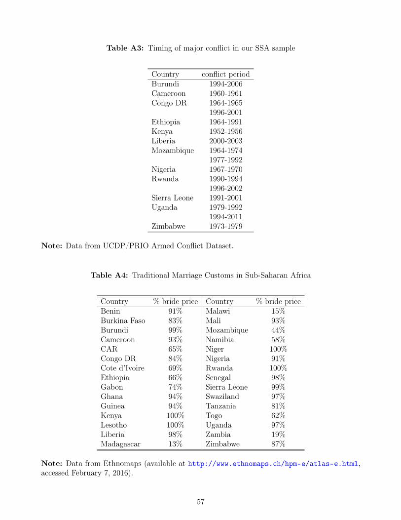
Table A3: Timing of major conflict in our SSA sample

Country conflict periodBurundi 1994-2006Cameroon 1960-1961Congo DR 1964-1965

1996-2001Ethiopia 1964-1991Kenya 1952-1956Liberia 2000-2003Mozambique 1964-1974

1977-1992Nigeria 1967-1970Rwanda 1990-1994

1996-2002Sierra Leone 1991-2001Uganda 1979-1992

1994-2011Zimbabwe 1973-1979

Note: Data from UCDP/PRIO Armed Conflict Dataset.

Table A4: Traditional Marriage Customs in Sub-Saharan Africa

Country % bride price Country % bride priceBenin 91% Malawi 15%Burkina Faso 83% Mali 93%Burundi 99% Mozambique 44%Cameroon 93% Namibia 58%CAR 65% Niger 100%Congo DR 84% Nigeria 91%Cote d’Ivoire 69% Rwanda 100%Ethiopia 66% Senegal 98%Gabon 74% Sierra Leone 99%Ghana 94% Swaziland 97%Guinea 94% Tanzania 81%Kenya 100% Togo 62%Lesotho 100% Uganda 97%Liberia 98% Zambia 19%Madagascar 13% Zimbabwe 87%

Note: Data from Ethnomaps (available at http://www.ethnomaps.ch/hpm-e/atlas-e.html,accessed February 7, 2016).

57

Figure A1: Crop Yields and Rainfall Vingtiles in Sub-Saharan Africa

(a) Average for Main Crops

-0.3

-0.2

-0.1

0.0

0.1

Coe

ffici

ent

1 2 3 4 5 6 7 8 9 12 13 14 15 16 17 18 19 20 (Omitted) Rain Vingtiles

Regression includes year and country FEs. SEs clustered at country level.

Coefficient for rain vingtiles and 95% CI in SSA: MainCrops

(b) Maize

-0.3

-0.2

-0.1

0.0

0.1

0.2

Coe

ffici

ent

1 2 3 4 5 6 7 8 9 12 13 14 15 16 17 18 19 20 (Omitted) Rain Vingtiles

Regression includes year and country FEs. SEs clustered at country level.

Coefficient for rain vingtiles and 95% CI in SSA: Maize

(c) Sorghum

-0.3

-0.2

-0.1

0.0

0.1

Coe

ffici

ent

1 2 3 4 5 6 7 8 9 12 13 14 15 16 17 18 19 20 (Omitted) Rain Vingtiles

Regression includes year and country FEs. SEs clustered at country level.

Coefficient for rain vingtiles and 95% CI in SSA: Sorghum

(d) Millet

-0.2

-0.1

0.0

0.1

0.2

Coe

ffici

ent

1 2 3 4 5 6 7 8 9 12 13 14 15 16 17 18 19 20 (Omitted) Rain Vingtiles

Regression includes year and country FEs. SEs clustered at country level.

Coefficient for rain vingtiles and 95% CI in SSA: Millet

(e) Rice

-0.3

-0.2

-0.1

0.0

0.1

0.2

Coe

ffici

ent

1 2 3 4 5 6 7 8 9 12 13 14 15 16 17 18 19 20 (Omitted) Rain Vingtiles

Regression includes year and country FEs. SEs clustered at country level.

Coefficient for rain vingtiles and 95% CI in SSA: Rice

(f) Wheat

-0.4

-0.2

0.0

0.2

0.4

Coe

ffici

ent

1 2 3 4 5 6 7 8 9 12 13 14 15 16 17 18 19 20 (Omitted) Rain Vingtiles

Regression includes year and country FEs. SEs clustered at country level.

Coefficient for rain vingtiles and 95% CI in SSA: Wheat

Note: Figure plots the coefficients of rainfall vingtiles in regressions with log of annual crop yield(tons per hectare) from 1961 to 2010 as the dependent variable. The sample consists of SSA countrieswith DHS surveys in our main analysis. The “Average for Main Crops” panel has the dependentvariable as the log of the sum of the total production of main crops reported (maize, wheat, sorghum,millet, and rice) divided by the total area harvested for those crops. The individual crop figuresare sorted by total production, averaged across the available years, from the most to the least. Allregression specifications include year and country fixed effects. The capped vertical bars show 95%confidence intervals calculated using robust standard errors clustered at the country level.

58

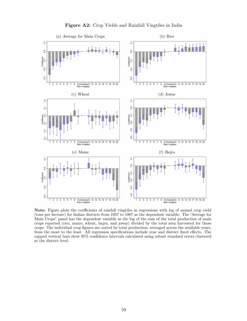
Figure A2: Crop Yields and Rainfall Vingtiles in India

(a) Average for Main Crops

-0.3

-0.2

-0.1

0.0

0.1

Coe

ffici

ent

1 2 3 4 5 6 7 8 9 12 13 14 15 16 17 18 19 20 (Omitted) Rain Vingtiles

Regression includes year and district FEs. SEs clustered at district level.

Coefficient for rain vingtiles and 95% CI in IN: MainCrops

(b) Rice

-0.3

-0.2

-0.1

0.0

0.1

Coe

ffici

ent

1 2 3 4 5 6 7 8 9 12 13 14 15 16 17 18 19 20 (Omitted) Rain Vingtiles

Regression includes year and district FEs. SEs clustered at district level.

Coefficient for rain vingtiles and 95% CI in IN: Rice

(c) Wheat

-0.1

-0.1

-0.1

0.0

0.1

0.1

Coe

ffici

ent

1 2 3 4 5 6 7 8 9 12 13 14 15 16 17 18 19 20 (Omitted) Rain Vingtiles

Regression includes year and district FEs. SEs clustered at district level.

Coefficient for rain vingtiles and 95% CI in IN: Wheat

(d) Jowar

-0.4

-0.3

-0.2

-0.1

0.0

0.1

Coe

ffici

ent

1 2 3 4 5 6 7 8 9 12 13 14 15 16 17 18 19 20 (Omitted) Rain Vingtiles

Regression includes year and district FEs. SEs clustered at district level.

Coefficient for rain vingtiles and 95% CI in IN: Jowar

(e) Maize

-0.3

-0.2

-0.1

0.0

0.1

Coe

ffici

ent

1 2 3 4 5 6 7 8 9 12 13 14 15 16 17 18 19 20 (Omitted) Rain Vingtiles

Regression includes year and district FEs. SEs clustered at district level.

Coefficient for rain vingtiles and 95% CI in IN: Maize

(f) Bajra

-0.4

-0.3

-0.2

-0.1

0.0

0.1

Coe

ffici

ent

1 2 3 4 5 6 7 8 9 12 13 14 15 16 17 18 19 20 (Omitted) Rain Vingtiles

Regression includes year and district FEs. SEs clustered at district level.

Coefficient for rain vingtiles and 95% CI in IN: Bajra

Note: Figure plots the coefficients of rainfall vingtiles in regressions with log of annual crop yield(tons per hectare) for Indian districts from 1957 to 1987 as the dependent variable. The “Average forMain Crops” panel has the dependent variable as the log of the sum of the total production of maincrops reported (rice, maize, wheat, bajra, and jowar) divided by the total area harvested for thosecrops. The individual crop figures are sorted by total production, averaged across the available years,from the most to the least. All regression specifications include year and district fixed effects. Thecapped vertical bars show 95% confidence intervals calculated using robust standard errors clusteredat the district level.

59

Table A5: Effect of Drought on Early Marriages (Extended Upper Age Cutoff)

SSA India: DHS India: DHS and IHDS

(1) (2) (3) (4) (5) (6) (7)Drought 0.0035*** 0.0035*** 0.0031*** -0.0060*** -0.0061*** -0.0029** -0.0029*

(0.00099) (0.00099) (0.00097) (0.0018) (0.0018) (0.0014) (0.0015)Birth Year FE Yes Yes Yes Yes Yes Yes YesAge FE Yes Yes Yes Yes Yes Yes YesCountry FE No Yes Yes No No No NoCountry FE × Cohort FE No No Yes No No No NoDistrict FE × Cohort FE No No No No Yes No YesN 3,236,694 3,236,694 3,236,694 838,846 838,846 610,669 610,669Adjusted R2 0.073 0.073 0.074 0.11 0.12 0.11 0.11

Note: * p<0.1, ** p<0.05, *** p<0.01Table shows OLS regressions for the full Sub-Saharan Africa (SSA) and India regression samples: women aged 25 or older at the timeof interview. Observations are at the level of person × age (from 10 to 24 or age of first marriage, whichever is earlier). Robuststandard errors (in parentheses) are clustered at the grid cell level in columns 1-3 and the district level in columns 4-5. All regressionspecifications include grid cell (SSA) or district (India) fixed effects. Results are weighted to be representative of the included countries(SSA) or districts (India).

60

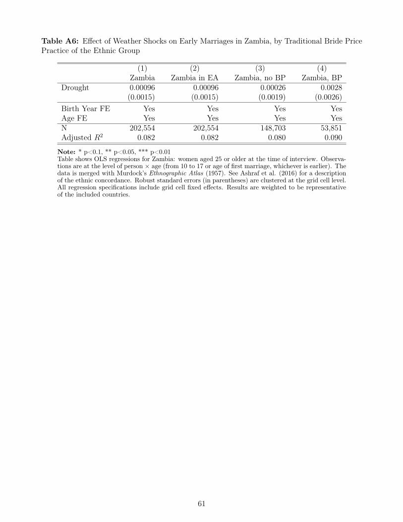
Table A6: Effect of Weather Shocks on Early Marriages in Zambia, by Traditional Bride PricePractice of the Ethnic Group

(1) (2) (3) (4)Zambia Zambia in EA Zambia, no BP Zambia, BP

Drought 0.00096 0.00096 0.00026 0.0028(0.0015) (0.0015) (0.0019) (0.0026)

Birth Year FE Yes Yes Yes YesAge FE Yes Yes Yes YesN 202,554 202,554 148,703 53,851Adjusted R2 0.082 0.082 0.080 0.090

Note: * p<0.1, ** p<0.05, *** p<0.01Table shows OLS regressions for Zambia: women aged 25 or older at the time of interview. Observa-tions are at the level of person × age (from 10 to 17 or age of first marriage, whichever is earlier). Thedata is merged with Murdock’s Ethnographic Atlas (1957). See Ashraf et al. (2016) for a descriptionof the ethnic concordance. Robust standard errors (in parentheses) are clustered at the grid cell level.All regression specifications include grid cell fixed effects. Results are weighted to be representativeof the included countries.

61

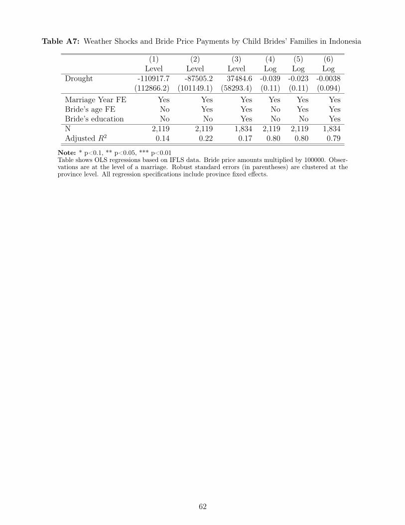
Table A7: Weather Shocks and Bride Price Payments by Child Brides’ Families in Indonesia

(1) (2) (3) (4) (5) (6)Level Level Level Log Log Log

Drought -110917.7 -87505.2 37484.6 -0.039 -0.023 -0.0038(112866.2) (101149.1) (58293.4) (0.11) (0.11) (0.094)

Marriage Year FE Yes Yes Yes Yes Yes YesBride’s age FE No Yes Yes No Yes YesBride’s education No No Yes No No YesN 2,119 2,119 1,834 2,119 2,119 1,834Adjusted R2 0.14 0.22 0.17 0.80 0.80 0.79

Note: * p<0.1, ** p<0.05, *** p<0.01Table shows OLS regressions based on IFLS data. Bride price amounts multiplied by 100000. Obser-vations are at the level of a marriage. Robust standard errors (in parentheses) are clustered at theprovince level. All regression specifications include province fixed effects.

62

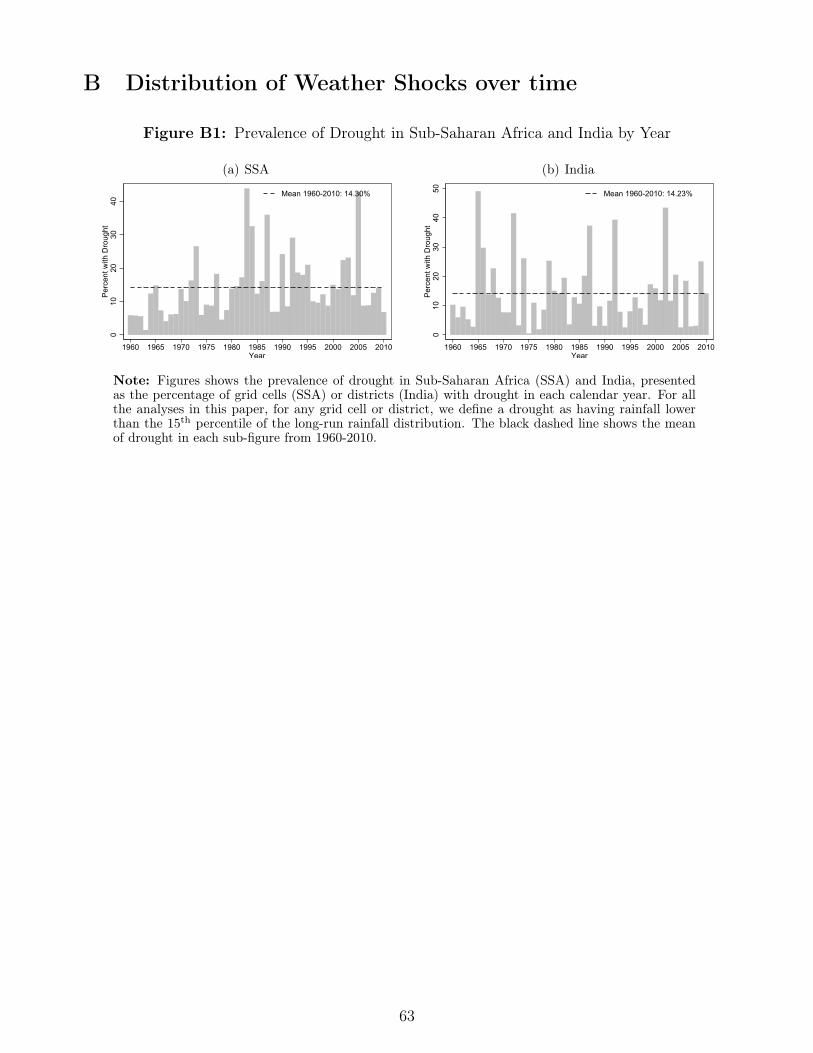
B Distribution of Weather Shocks over time

Figure B1: Prevalence of Drought in Sub-Saharan Africa and India by Year

(a) SSA

010

2030

40P

erce

nt w

ith D

roug

ht

1960 1965 1970 1975 1980 1985 1990 1995 2000 2005 2010Year

Mean 1960-2010: 14.30%

Figure shows the percent of grid cells in SSA with drought each year.The dashed black line indicates the long run mean from 1960 to 2010.

Prevalence of Drought: SSA (b) India

010

2030

4050

Per

cent

with

Dro

ught

1960 1965 1970 1975 1980 1985 1990 1995 2000 2005 2010Year

Mean 1960-2010: 14.23%

Figure shows the percent of grid cells in India with drought each year.The dashed black line indicates the long run mean from 1960 to 2010.

Prevalence of Drought: India

Note: Figures shows the prevalence of drought in Sub-Saharan Africa (SSA) and India, presentedas the percentage of grid cells (SSA) or districts (India) with drought in each calendar year. For allthe analyses in this paper, for any grid cell or district, we define a drought as having rainfall lowerthan the 15th percentile of the long-run rainfall distribution. The black dashed line shows the meanof drought in each sub-figure from 1960-2010.

63

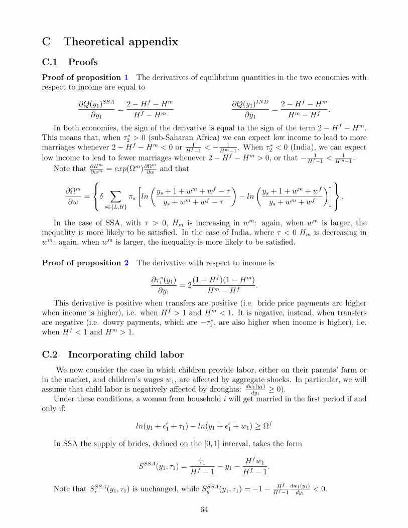
C Theoretical appendix

C.1 Proofs

Proof of proposition 1 The derivatives of equilibrium quantities in the two economies withrespect to income are equal to

∂Q(y1)SSA

∂y1

=2−Hf −Hm

Hf −Hm

∂Q(y1)IND

∂y1

=2−Hf −Hm

Hm −Hf.

In both economies, the sign of the derivative is equal to the sign of the term 2−Hf −Hm.This means that, when τ ∗2 > 0 (sub-Saharan Africa) we can expect low income to lead to moremarriages whenever 2−Hf −Hm < 0 or 1

Hf−1< − 1

Hm−1. When τ ∗2 < 0 (India), we can expect

low income to lead to fewer marriages whenever 2−Hf −Hm > 0, or that − 1Hf−1

< 1Hm−1

.Note that ∂Hm

∂wm= exp(Ωm)∂Ωm

∂wand that

∂Ωm

∂w=

δ ∑s∈L,H

πs

[ln

(ys + 1 + wm + wf − τys + wm + wf − τ

)− ln

(ys + 1 + wm + wf

ys + wm + wf

)] .

In the case of SSA, with τ > 0, Hm is increasing in wm: again, when wm is larger, theinequality is more likely to be satisfied. In the case of India, where τ < 0 Hm is decreasing inwm: again, when wm is larger, the inequality is more likely to be satisfied.

Proof of proposition 2 The derivative with respect to income is

∂τ ∗1 (y1)

∂y1

= 2(1−Hf )(1−Hm)

Hm −Hf.

This derivative is positive when transfers are positive (i.e. bride price payments are higherwhen income is higher), i.e. when Hf > 1 and Hm < 1. It is negative, instead, when transfersare negative (i.e. dowry payments, which are −τ ∗1 , are also higher when income is higher), i.e.when Hf < 1 and Hm > 1.

C.2 Incorporating child labor

We now consider the case in which children provide labor, either on their parents’ farm orin the market, and children’s wages w1, are affected by aggregate shocks. In particular, we willassume that child labor is negatively affected by droughts: dw1(y1)

dy1≥ 0).

Under these conditions, a woman from household i will get married in the first period if andonly if:

ln(y1 + εi1 + τ1)− ln(y1 + εi1 + w1) ≥ Ωf

In SSA the supply of brides, defined on the [0, 1] interval, takes the form

SSSA(y1, τ1) =τ1

Hf − 1− y1 −

Hfw1

Hf − 1.

Note that SSSAτ (y1, τ1) is unchanged, while SSSAy (y1, τ1) = −1− Hf

Hf−1dw1(y1)dy1

< 0.

64

Similarly, under these conditions, a man from household i will get married in the first periodif and only if:

ln(y1 + εj1 − τ1 + 2w1)− ln(y1 + εj1 + w1) ≥ Ωf .

Hence, the demand for brides becomes

DSSA(y1, τ1) = 1 + y1 +τ1

Hm − 1+Hm − 2

Hm − 1w1.

Again, the derivative with respect to prices is unchanged, while DSSAy (y1, τ1) = 1+Hm−2

Hm−1dw1(y1)dy1

>0.

In India, the supply of brides, defined on the [0, 1] interval, takes the form

SIND(y1, τ1) = 1− τ1

Hf − 1+ y1 +

Hfw1

Hf − 1.

Here, SINDy (y1, τ1) = 1 + Hf

Hf−1dw1(y1)dy1

, which cannot be signed: droughts reduce parent’s abilityto pay dowry, but also makes a child daughter’s labor less valuable to the household.

The demand for brides becomes

DIND(y1, τ1) = −y1 −τ1

Hm − 1− Hm − 2

Hm − 1w1.

Again, the derivative with respect to prices is unchanged, whileDINDy (y1, τ1) = −1−Hm−2

Hm−1dw1(y1)dy1

.Equilibrium quantities are :

Q(y1)SSA =2−Hf −Hm

Hf −Hm(y1 + w1)− Hm − 1

Hf −Hm,

Q(y1)IND =2−Hf −Hm

Hm −Hf(y1 + w1)− Hf − 1

Hm −Hf.

The derivatives of these quantities with respect to aggregate income are

∂Q(y1)SSA

∂y1

=2−Hf −Hm

Hf −Hm

(1 +

dw1(y1)

dy1

)∂Q(y1)IND

∂y1

=2−Hf −Hm

Hm −Hf

(1 +

dw1(y1)

dy1

).

Hence, as long as dw1(y1)dy1

≥ 0, the proof of proposition 1 continues to hold and the effect ofdrought on the quantity of child marriages is stronger. This effect happens because families ofboys are affected less strongly by the drought even in the first period, because they can rely ontheir child son’s labor even if he gets married.

Equilibrium marriage payments are

τ ∗1 (y1) =(Hf − 1)(Hm − 1)

Hm −Hf(1 + 2y1) +

(2Hf − Hm − 2

Hm −Hf

)w.

65

The derivative with respect to income is

∂τ ∗1 (y1)

∂y1

= 2(Hf − 1)(Hm − 1)

Hm −Hf+

(2Hf − Hm − 2

Hm −Hf

)dw1(y1)

dy1

.

Hence, predictions about equilibrium marriage payments with child labor are ambiguous.Proposition 2 may not hold, but price effects are no longer necessary to obtain quantity effects.

C.3 Generalizing preferences and distributions

Consider general preferences represented by a function u(·) which is strictly increasing,strictly concave and twice-continuously differentiable. For proposition 1 to hold, we will alsorequire that households are prudent (u′′′(·) > 0). Allow also the distribution of εt to follow acontinuous distribution with pdf f(·) and cdf F (·) for both men and women.

As in the log-utility case, a woman from household i will get married in the first period ifand only if:

u(y1 + εi1 + τ1) + δE[u(y2 + εi2)

]≥ u(y1 + εi1) + δE

[u(y2 + εi2 + τ ∗2 )

]Similarly, a man from household j will get married in the first period if and only if:

u(y1 + εj1 − τ1) + δE[u(y2 + εj2 + wm + wf )

]≥

u(y1 + εj1) + δE[u(y2 + εj2 + wm + wf − τ ∗2 )

].

Consider now the income thresholds ε∗f and ε∗m at which the above expressions hold withequality:

u(y1 + εf∗1 + τ1)− u(y1 + εf∗1 ) = Ωf

u(y1 + εm∗ − τ1)− u(y1 + εm∗) = Ωm.

Define Ωf = δE [u(y2 + εi2 + τ ∗2 )]−δE [u(y2 + εi2)] and Ωm = δE[u(y2 + εj2 + wm + wf − τ ∗2 )

]−

δE[u(y2 + εj2 + wm + wf )

]. Applying the implicit function theorem (IFT) and the chain rule,

we have that

∂ε∗f (τ1, y1,Ωf )

∂τ1

= −u′(y1 + ε∗f + τ1)

u′(y1 + ε∗f + τ1)− u′(y1 + ε∗f )

∂ε∗f (τ1, y1,Ωf )

∂y1

= −u′(y1 + ε∗f + τ1)− u′(y1 + ε∗f )

u′(y1 + ε∗f + τ1)− u′(y1 + ε∗f )= −1

∂ε∗m(τ1, y1,Ωm)

∂τ1

=u′(y1 + ε∗m − τ1)

u′(y1 + ε∗m − τ1)− u′(y1 + ε∗m)

∂ε∗m(τ1, y1,Ωm)

∂y1

= −u′(y1 + ε∗m − τ1)− u′(y1 + ε∗m)

u′(y1 + ε∗m − τ1)− u′(y1 + ε∗m)= −1.

Sub-Saharan Africa Monotonicity and concavity of the utility function, as well as the factthat continuation values do not depend on εi1, imply that below threshold ε∗f every household

66

wants their daughter to be married, ceteris paribus. This implies that the supply of brides isdefined in SSA as:

SSSA(τ1, y1,Ωf ) = Prob(εit < ε∗f (τ1, y1,Ω

f )) = F (ε∗f (τ1, y1,Ωf )).

Concavity ensures that∂ε∗f (τ1,y1,Ωf )

∂τ1> 0.

The above conditions, together with the chain rule and the fact that F ′(·) = f(·) > 0, alsoimply that

∂SSSA(τ1, y1,Ωf )

∂τ1

= SSSAτ (τ1, y1,Ωf ) = f(ε∗f (τ1, y1,Ω

f ))∂ε∗f (τ1, y1,Ω

f )

∂τ1

> 0

∂SSSA(τ1, y1,Ωf )

∂y1

= SSSAy (τ1, y1,Ωf ) = −f(ε∗f (τ1, y1,Ω

f )) < 0.

A similar argument would lead us to show that the demand for brides is

DSSA(τ1, y1,Ωm) = Prob(εi ≥ ε∗m(τ1, y1,Ω

m)) = 1− F (ε∗m(τ1, y1,Ωm))

and the derivative of the threshold with respect to the marriage payment is ∂ε∗m(τ1,y1,Ωm)∂τ1

> 0.Hence, because of continuity and the chain rule

∂DSSA(τ1, y1,Ωm)

∂τ1

= DSSAτ (τ1, y1,Ω

m) = −f(ε∗m(τ1, y1,Ωm))

∂ε∗m(τ1, y1,Ωm)

∂τ1

< 0

∂DSSA(τ1, y1,Ωm)

∂y1

= DSSAy (τ1, y1,Ω

m) = f(ε∗m(τ1, y1,Ωm)) > 0.

India The same arguments used above, when transfers are negative, would lead us to concludethat

∂ε∗f (τ1,y1,Ωf )

∂τ1< 0 and ∂ε∗m(τ1,y1,Ωm)

∂τ1< 0. Hence

SIND(τ1, y1,Ωf ) = Prob(εi ≥ ε∗f (τ1, y1,Ω

f )) = 1− F (ε∗f (τ1, y1,Ωf ))

DIND(τ1, y1,Ωm) = Prob(εi < ε∗m(τ1, y1,Ω

m)) = F (ε∗m(τ1, y1,Ωm)).

The derivatives are the following:

∂SIND(τ1, y1,Ωf )

∂τ1

= SINDτ (τ1, y1,Ωf ) = −f(ε∗f (τ1, y1,Ω

f ))∂ε∗f (τ1, y1,Ω

f )

∂τ1

> 0

∂SIND(τ1, y1,Ωf )

∂y1

= SINDy (τ1, y1,Ωf ) = f(ε∗f (τ1, y1,Ω

f )) > 0

∂DIND(τ1, y1,Ωm)

∂τ1

= DINDτ (τ1, y1,Ω

m) = f(ε∗m(τ1, y1,Ωm))

∂ε∗m(τ1, y1,Ωm)

∂τ1

< 0

∂DIND(τ1, y1,Ωm)

∂y1

= DINDy (τ1, y1,Ω

m) = −f(ε∗m(τ1, y1,Ωm)) < 0.

67

Equilibrium In both economies, equilibrium prices are defined implicitly as the solution to

S(τ ∗1 , y1,Ωf )−D(τ ∗1 , y1,Ω

m) = 0.

By the IFT, the derivative of the equilibrium price with respect to y1 is

∂τ ∗1∂y1

= −Sy(τ1, y1,Ωf )−Dy(τ1, y1,Ω

m)

Sτ (τ1, y1,Ωf )−Dτ (τ1, y1,Ωm).

This derivative is positive in SSA and negative in India (as stated in proposition 2).Define now τ = S−1(q1, y1,Ω

f ) as an inverse supply function and τ = D−1(q1, y1,Ωm) as an

inverse demand function. Note that S−1q (q, y1,Ω

f ) and D−1q (q, y1,Ω

m) have the same sign asSτ (τ1, y1,Ω

f ) (positive) and Dτ (τ1, y1,Ωm) (negative), respectively. Moreover, S−1

y (q, y1,Ωf ) =

−Sy(τ1,y1,Ωf )

Sτ (τ1,y1,Ωf )is positive SSA and negative in India, as is D−1

y (q, y1,Ωm) = −Dy(τ1,y1,Ωm)

Dτ (τ1,y1,Ωm).15

In equilibrium, D−1(Q, y1,Ωm) = τ ∗ = S−1(Q, y1,Ω

f ) where Q is the equilibrium quantityof child marriage. Again the IFT allows us to derive

Q′(y1) = −S−1y (Q, y1,Ω

f )−D−1y (Q, y1,Ω

m)

S−1q (Q, y1,Ωf )−D−1

q (Q, y1,Ωm).

The denominator of the above expression, S−1,SSAq (Q, y1,Ω

f ) − D−1,SSAq (Q, y1, w

m,Ωm), isalways positive.

Hence, in SSA, in order to have that Q′(y1) < 0, we need that S−1,SSAy (Q, y1,Ω

f ) >

D−1,SSAy (Q, y1,Ω

m), hence that −SSSAy (τ1,y1,Ωf )

SSSAτ (τ1,y1,Ωf )> −DSSAy (τ1,y1,Ωm)

DSSAτ (τ1,y1,Ωm)or

SSSAy (τ1, y1,Ωf )

SSSAτ (τ1, y1,Ωf )<DSSAy (τ1, y1,Ω

m)

DSSAτ (τ1, y1,Ωm)

.

Applying the above derivations of these partial derivatives, we have that:

SSSAy (τ1, y1,Ωf )

SSSAτ (τ1, y1,Ωf )= − 1

∂ε∗f (τ1,y1,Ωf )

∂τ1

and

DSSAy (τ1, y1,Ω

m)

DSSAτ (τ1, y1,Ωm)

=f(ε∗m(τ1, y1,Ω

m))

−f(ε∗m(τ1, y1,Ωm))∂ε∗m(τ1,y1,Ωm)

∂τ1

= − 1∂ε∗m(τ1,y1,Ωm)

∂τ1

.

Hence, the condition translates into

∂ε∗f (τ1, y1,Ωf )

∂τ1

<∂ε∗m(τ1, y1,Ω

m)

∂τ1

,

In India, in order to have that Q′(y1) > 0, we need that S−1,INDy (Q, y1) < D−1,IND

y (Q, y1),

hence that −SINDy (τ1,y1,Ωf )

SINDτ (τ1,y1,Ωf )< −DINDy (τ1,y1,Ωm)

DINDτ (τ1,y1,Ωm)or

SINDy (τ1, y1,Ωf )

SINDτ (τ1, y1,Ωf )>DINDy (τ1, y1,Ω

m)

DINDτ (τ1, y1,Ωm)

.

15To see this, consider the conditions q − S(τ1, y1,Ωf ) = 0 and q −D(τ1, y1,Ω

m) = 0 and apply the IFT.

68

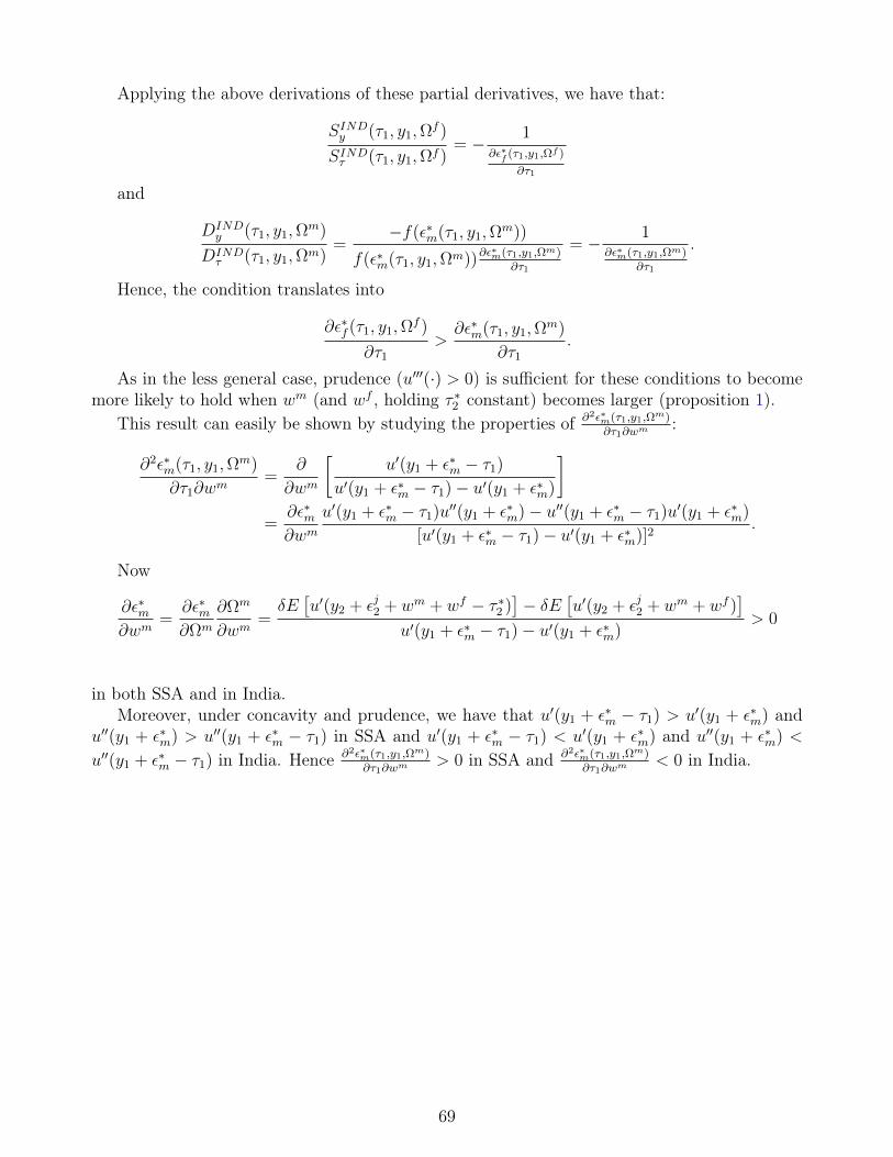
Applying the above derivations of these partial derivatives, we have that:

SINDy (τ1, y1,Ωf )

SINDτ (τ1, y1,Ωf )= − 1

∂ε∗f (τ1,y1,Ωf )

∂τ1

and

DINDy (τ1, y1,Ω

m)

DINDτ (τ1, y1,Ωm)

=−f(ε∗m(τ1, y1,Ω

m))

f(ε∗m(τ1, y1,Ωm))∂ε∗m(τ1,y1,Ωm)

∂τ1

= − 1∂ε∗m(τ1,y1,Ωm)

∂τ1

.

Hence, the condition translates into

∂ε∗f (τ1, y1,Ωf )

∂τ1

>∂ε∗m(τ1, y1,Ω

m)

∂τ1

.

As in the less general case, prudence (u′′′(·) > 0) is sufficient for these conditions to becomemore likely to hold when wm (and wf , holding τ ∗2 constant) becomes larger (proposition 1).

This result can easily be shown by studying the properties of ∂2ε∗m(τ1,y1,Ωm)∂τ1∂wm

:

∂2ε∗m(τ1, y1,Ωm)

∂τ1∂wm=

∂

∂wm

[u′(y1 + ε∗m − τ1)

u′(y1 + ε∗m − τ1)− u′(y1 + ε∗m)

]=

∂ε∗m∂wm

u′(y1 + ε∗m − τ1)u′′(y1 + ε∗m)− u′′(y1 + ε∗m − τ1)u′(y1 + ε∗m)

[u′(y1 + ε∗m − τ1)− u′(y1 + ε∗m)]2.

Now

∂ε∗m∂wm

=∂ε∗m∂Ωm

∂Ωm

∂wm=δE[u′(y2 + εj2 + wm + wf − τ ∗2 )

]− δE

[u′(y2 + εj2 + wm + wf )

]u′(y1 + ε∗m − τ1)− u′(y1 + ε∗m)

> 0

in both SSA and in India.Moreover, under concavity and prudence, we have that u′(y1 + ε∗m − τ1) > u′(y1 + ε∗m) and

u′′(y1 + ε∗m) > u′′(y1 + ε∗m − τ1) in SSA and u′(y1 + ε∗m − τ1) < u′(y1 + ε∗m) and u′′(y1 + ε∗m) <

u′′(y1 + ε∗m − τ1) in India. Hence ∂2ε∗m(τ1,y1,Ωm)∂τ1∂wm

> 0 in SSA and ∂2ε∗m(τ1,y1,Ωm)∂τ1∂wm

< 0 in India.

69