Chi-Squared Significance Tests

Chapters 26/27

Objectives:

• Chi-Squared Distribution• Chi-Squared Test Statistic• Chi-Squared Goodness of Fit Test• Chi-Squared Test of Independence

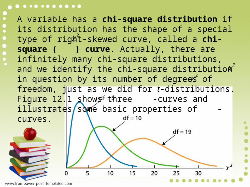
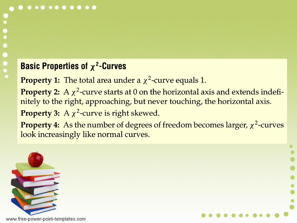
A variable has a chi-square distribution if its distribution has the shape of a special type of right-skewed curve, called a chi-square ( ) curve. Actually, there are infinitely many chi-square distributions, and we identify the chi-square distribution in question by its number of degrees of freedom, just as we did for t-distributions. Figure 12.1 shows three

-curves and illustrates some basic properties of -curves.

2

2

2

Chi-Square Table

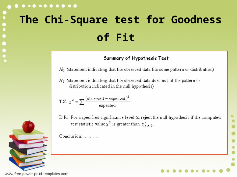
Chi-Square (2) Test for Goodness of Fit

Definition

Goodness-of-fit test

A goodness-of-fit test is used to test the hypothesis that an observed frequency distribution fits (or conforms to) some claimed distribution.

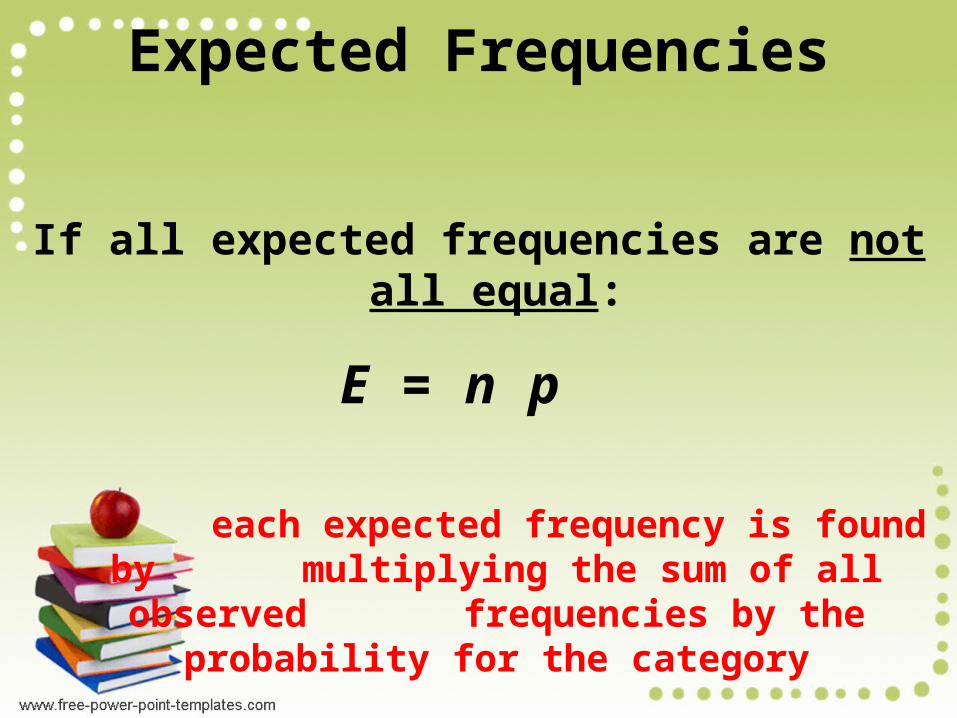
Expected Frequencies

If all expected frequencies are not all equal:

each expected frequency is found by multiplying the sum of all observed frequencies by the probability for the

category

E = n p

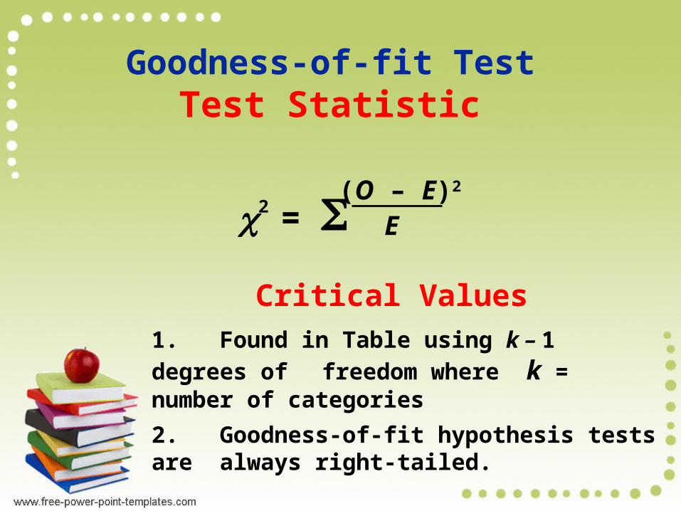
Goodness-of-fit Test Test Statistic

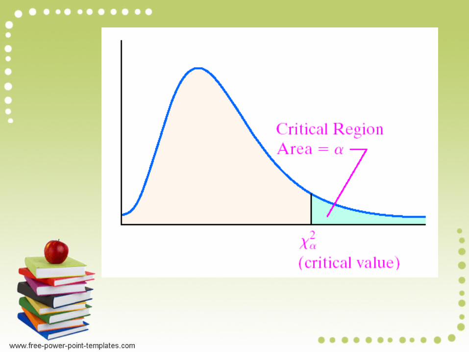
Critical Values1. Found in Table using k – 1 degrees of

freedom where k = number of categories

2. Goodness-of-fit hypothesis tests are always right-tailed.

2 = (O – E)2

E

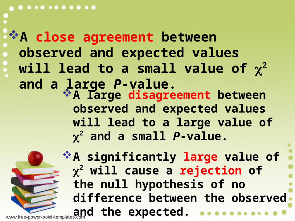
A large disagreement between observed and expected values will lead to a large value of 2 and a small P-value.

A significantly large value of 2 will cause a rejection of the null hypothesis of no difference between the observed and the expected.

A close agreement between observed and expected values will lead to a small value of 2 and a large P-value.

ExampleThe U.S. Federal Bureau of Investigation (FBI) compiles data on crimes and crime rates and publishes the information in Crime in the United States. A violent crime is classified by the FBI as murder, forcible rape, robbery, or aggravated assault. Table 12.1 gives a relative-frequency distribution for (reported) violent crimes in 2000. For instance, in 2000, 28.6% of violent crimes were robberies.A random sample of 500 violent-crime reports from last year yielded the frequency distribution shown in Table 12.2. Suppose that we want to use the data in Tables 12.1 and 12.2 to decide whether last year’s distribution of violent crimes has changed from the 2000 distribution.

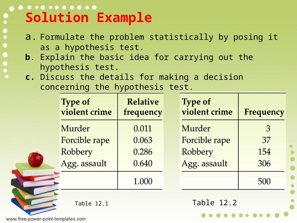
Table 12.1 Table 12.2

Solution Examplea. Formulate the problem statistically by posing it as a hypothesis

test.b. Explain the basic idea for carrying out the hypothesis test.c. Discuss the details for making a decision concerning the

hypothesis test.

Solution Example

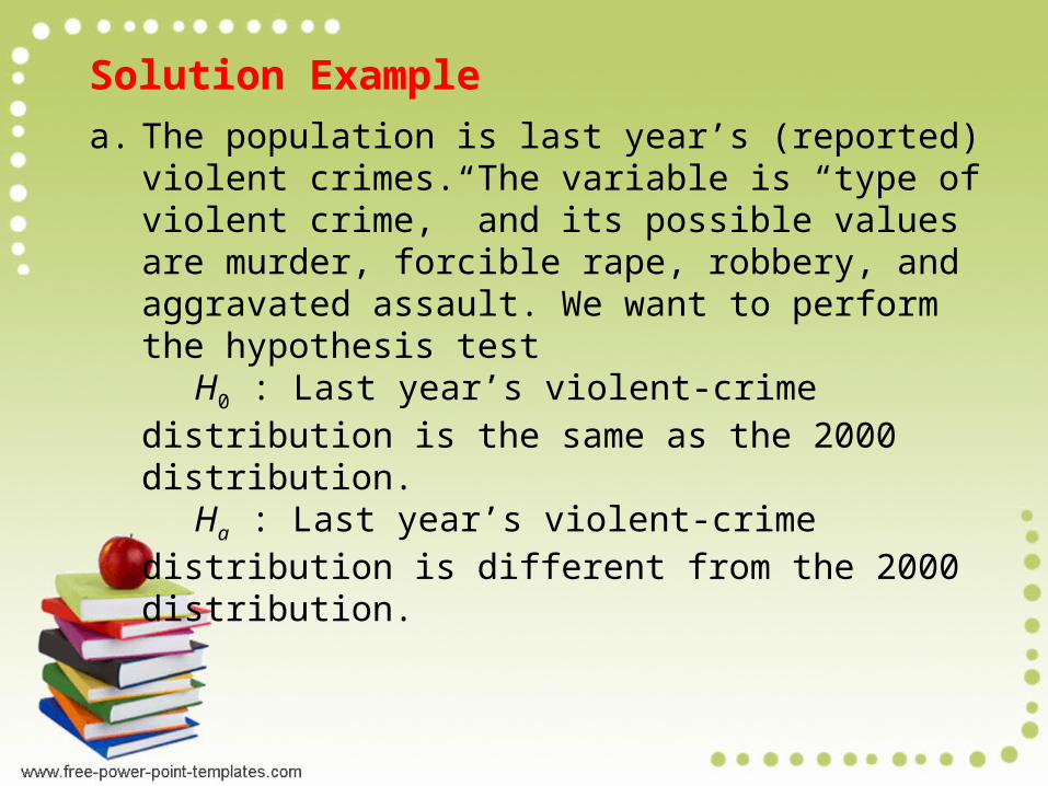
a. The population is last year’s (reported) violent crimes. The variable is “type of violent crime,” and its possible values are murder, forcible rape, robbery, and aggravated assault. We want to perform the hypothesis test

H0 : Last year’s violent-crime distribution is the same as the 2000 distribution.

Ha : Last year’s violent-crime distribution is different from the 2000 distribution.

Solution Example

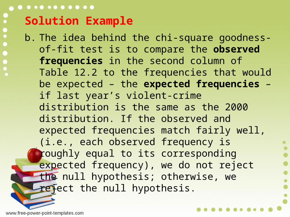
b. The idea behind the chi-square goodness-of-fit test is to compare the observed frequencies in the second column of Table 12.2 to the frequencies that would be expected – the expected frequencies – if last year’s violent-crime distribution is the same as the 2000 distribution. If the observed and expected frequencies match fairly well, (i.e., each observed frequency is roughly equal to its corresponding expected frequency), we do not reject the null hypothesis; otherwise, we reject the null hypothesis.

Solution Example

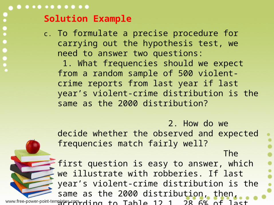
c. To formulate a precise procedure for carrying out the hypothesis test, we need to answer two questions: 1. What frequencies should we expect from a random sample of 500 violent-crime reports from last year if last year’s violent-crime distribution is the same as the 2000 distribution? 2. How do we decide whether the observed and expected frequencies match fairly well? The first question is easy to answer, which we illustrate with robberies. If last year’s violent-crime distribution is the same as the 2000 distribution, then, according to Table 12.1, 28.6% of last year’s violent crimes would have been robberies. Therefore, in a random sample of 500 violent-crime reports from last year, we would expect about 28.6% of the 500, or 143, to be robberies.

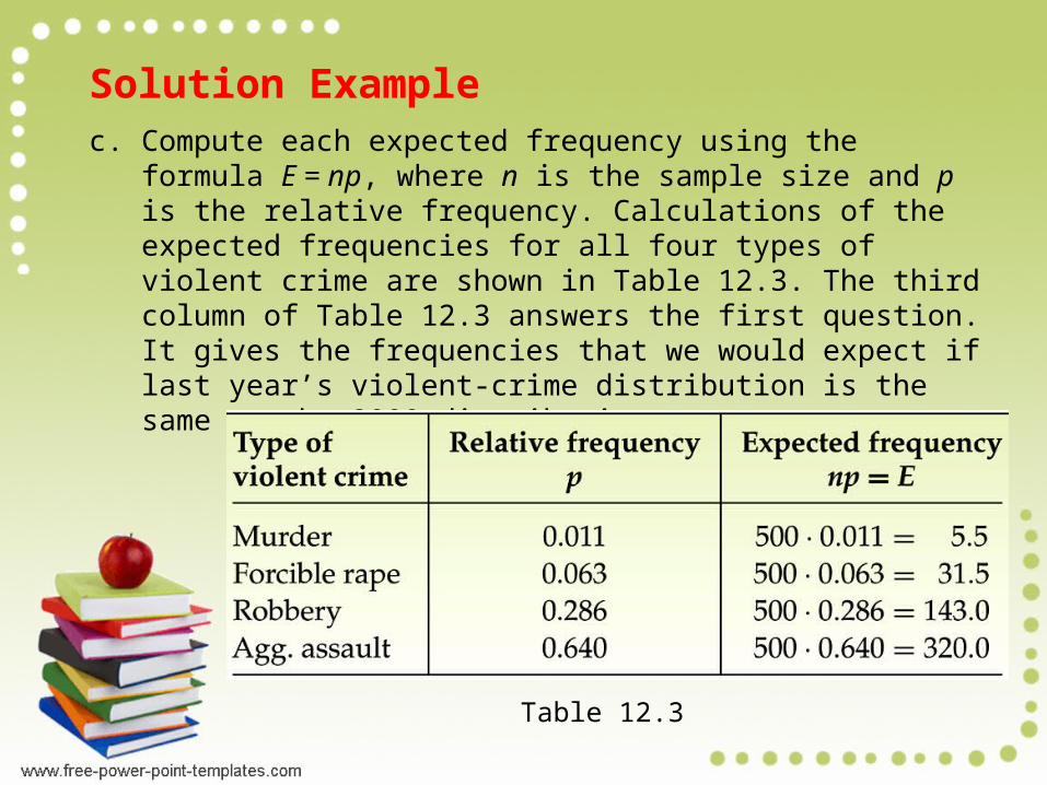
Solution Examplec. Compute each expected frequency using the formula E = np,

where n is the sample size and p is the relative frequency. Calculations of the expected frequencies for all four types of violent crime are shown in Table 12.3. The third column of Table 12.3 answers the first question. It gives the frequencies that we would expect if last year’s violent-crime distribution is the same as the 2000 distribution.

Table 12.3

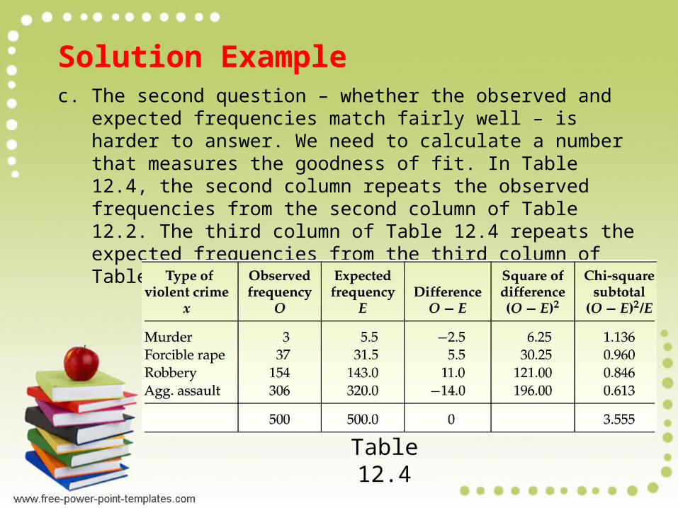
Solution Examplec. The second question – whether the observed and expected

frequencies match fairly well – is harder to answer. We need to calculate a number that measures the goodness of fit. In Table 12.4, the second column repeats the observed frequencies from the second column of Table 12.2. The third column of Table 12.4 repeats the expected frequencies from the third column of Table 12.3.

Table 12.4

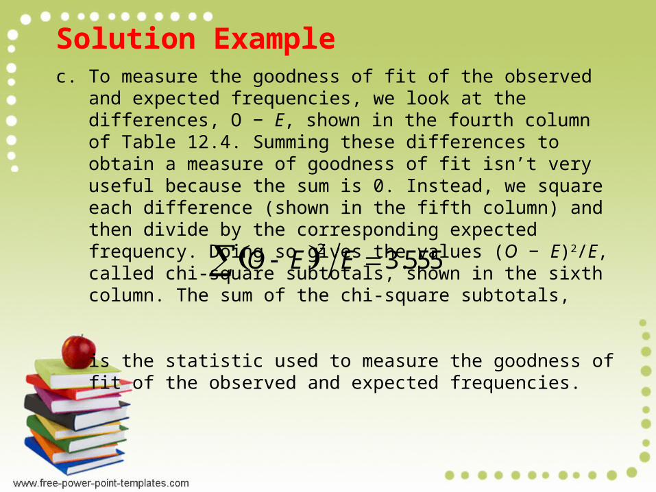
Solution Examplec. To measure the goodness of fit of the observed and expected

frequencies, we look at the differences, O − E, shown in the fourth column of Table 12.4. Summing these differences to obtain a measure of goodness of fit isn’t very useful because the sum is 0. Instead, we square each difference (shown in the fifth column) and then divide by the corresponding expected frequency. Doing so gives the values (O − E)2/E, called chi-square subtotals, shown in the sixth column. The sum of the chi-square subtotals,

is the statistic used to measure the goodness of fit of the observed and expected frequencies.

O E 2 E 3.555

Solution Examplec. If the null hypothesis is true, the observed and expected

frequencies should be roughly equal, resulting in a small value of the test statistic,

(O − E)2/E. In other words, large values of

(O − E)2/E provide evidence against the null hypothesis.

As we have seen, (O − E)2/E = 3.555. Can this value be reasonably attributed to sampling error, or is it large enough to suggest that the null hypothesis is false? To answer this question, we need to know the distribution of the

test statistic (O − E)2/E.

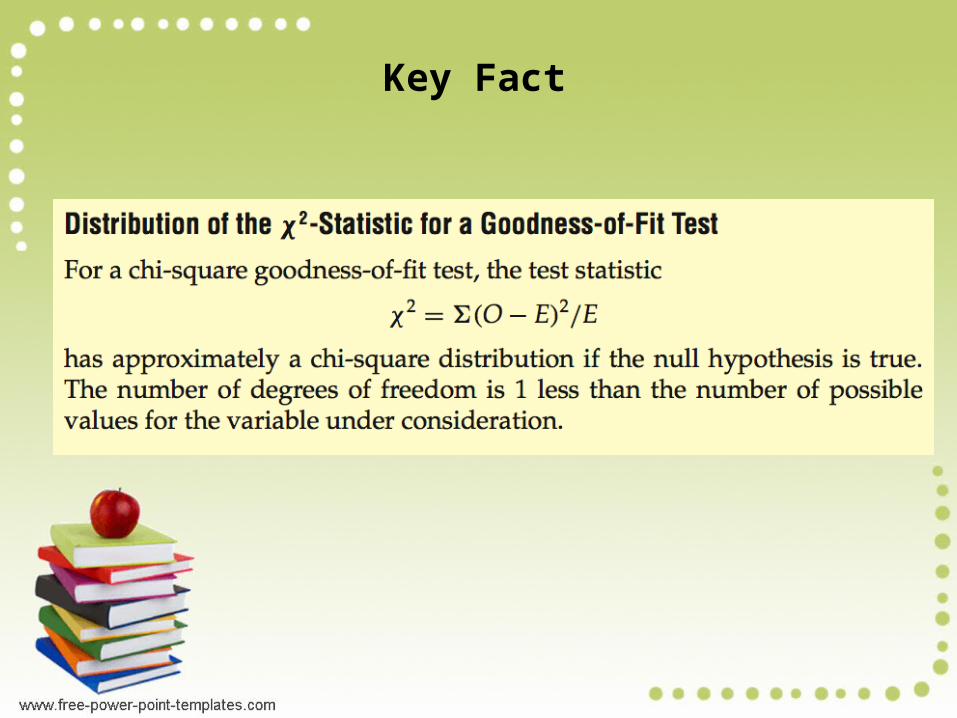
Key Fact

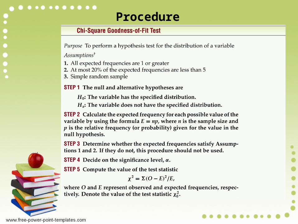
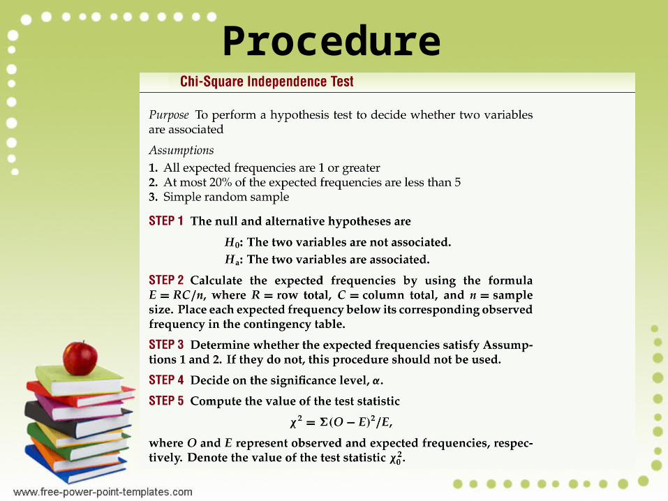
Procedure

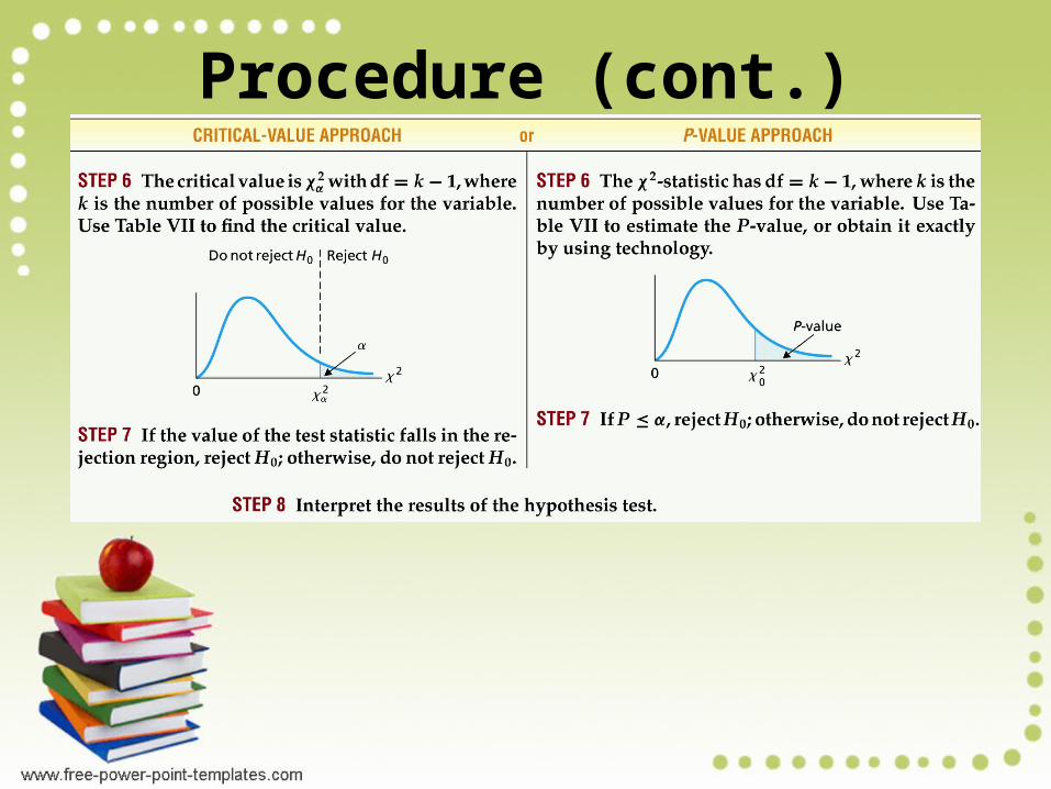
Procedure (cont.)

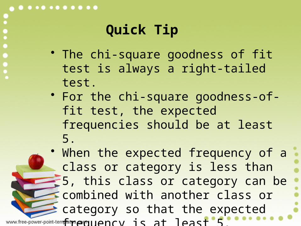
Quick Tip • The chi-square goodness of fit test is

always a right-tailed test. • For the chi-square goodness-of-fit

test, the expected frequencies should be at least 5.

• When the expected frequency of a class or category is less than 5, this class or category can be combined with another class or category so that the expected frequency is at least 5.

EXAMPLE • There are 4 TV sets that are located in

the student center of a large university. At a particular time each day, four different soap operas (1, 2, 3, and 4) are viewed on these TV sets. The percentages of the audience captured by these shows during one semester were 25 percent, 30 percent, 25 percent, and 20 percent, respectively. During the first week of the following semester, 300 students are surveyed.

EXAMPLE

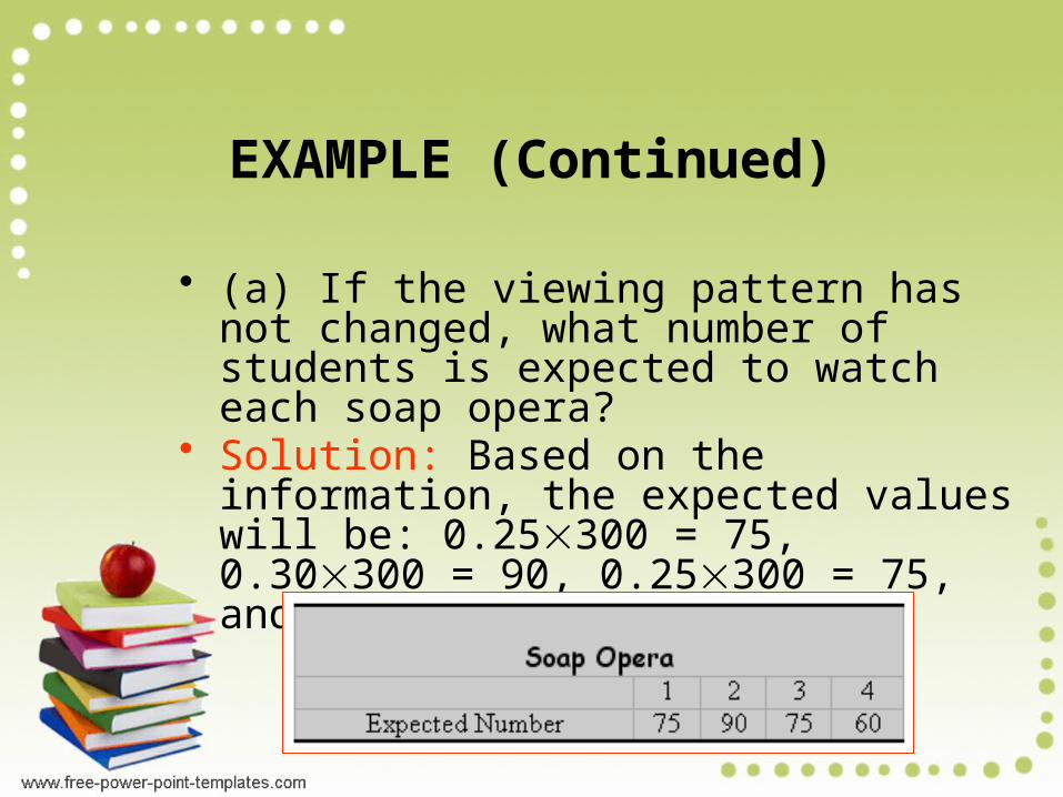
(Continued) • (a) If the viewing pattern has not

changed, what number of students is expected to watch each soap opera?

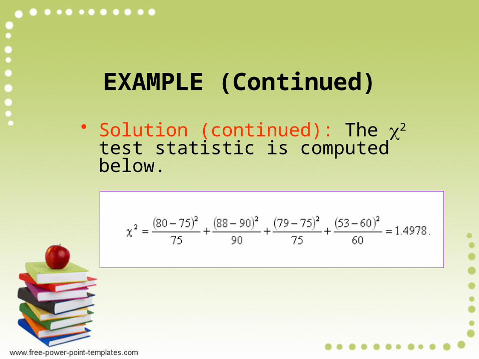
• Solution: Based on the information, the expected values will be: 0.25300 = 75, 0.30300 = 90, 0.25300 = 75, and 0.20300 = 60.

EXAMPLE

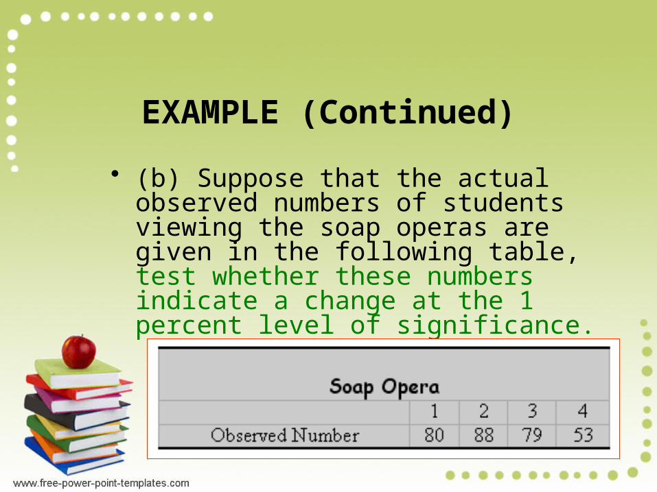
(Continued) • (b) Suppose that the actual observed

numbers of students viewing the soap operas are given in the following table, test whether these numbers indicate a change at the 1 percent level of significance.

EXAMPLE

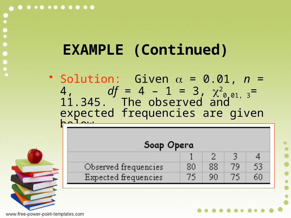
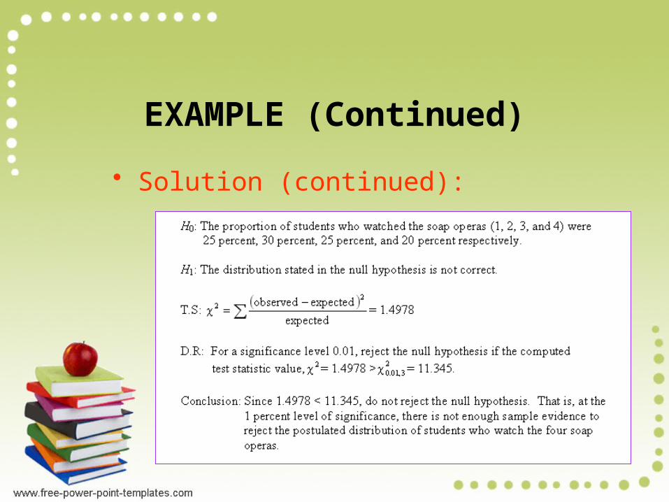
(Continued) • Solution: Given = 0.01, n = 4, df

= 4 – 1 = 3, 20.01, 3= 11.345. The

observed and expected frequencies are given below

EXAMPLE

(Continued) • Solution (continued): The 2 test

statistic is computed below.

EXAMPLE

(Continued) • Solution (continued):

EXAMPLE

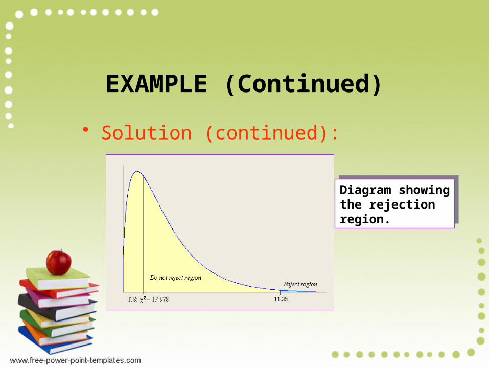
(Continued) • Solution (continued):

Diagram showingthe rejectionregion.

Diagram showingthe rejectionregion.

The Chi-Square test for Goodness

of Fit

2 Test of Independence

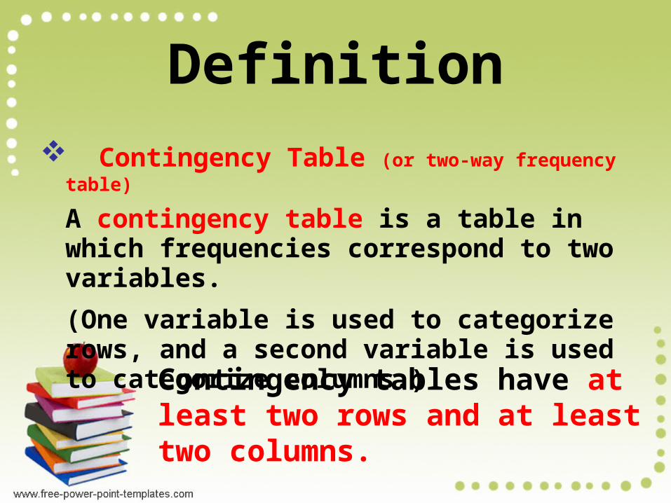
Definition Contingency Table (or two-way frequency table)

A contingency table is a table in which frequencies correspond to two variables.

(One variable is used to categorize rows, and a second variable is used to categorize columns.)

Contingency tables have at least two rows and at least two columns.

Definition

Test of Independence This method tests the null

hypothesis that the row variable and column variable in a contingency table are not related. (The null hypothesis is the statement that the row and column variables are independent.)

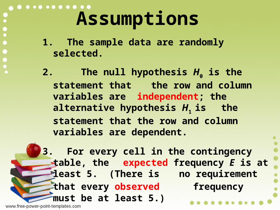
Assumptions1. The sample data are randomly selected.

2. The null hypothesis H0 is the statement

that the row and column variables are independent; the alternative hypothesis H1 is

the statement that the row and column variables are dependent.

3. For every cell in the contingency table, the expected frequency E is at least 5. (There is no requirement that every observed

frequency must be at least 5.)

Test of IndependenceTest Statistic

Critical Values1. Found in Table using

degrees of freedom = (r – 1)(c – 1)

r is the number of rows and c is the number of columns

2. Tests of Independence are always right-tailed.

2 = (O – E)2

E

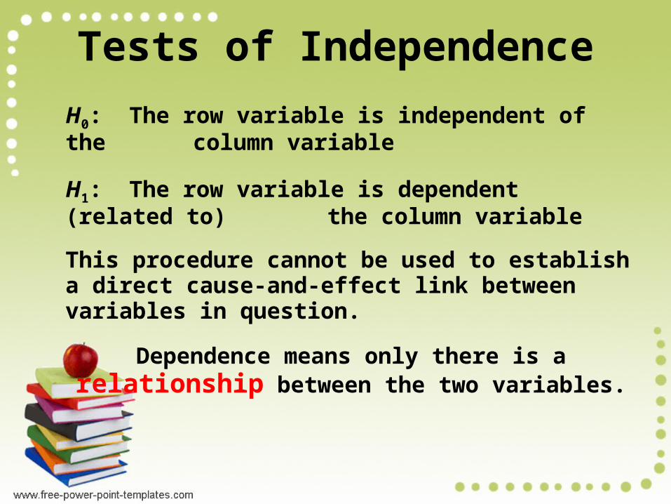
Tests of Independence

H0: The row variable is independent of the column variable

H1: The row variable is dependent (related to) the column variable

This procedure cannot be used to establish a direct cause-and-effect link between variables in question.

Dependence means only there is a relationship between the two variables.

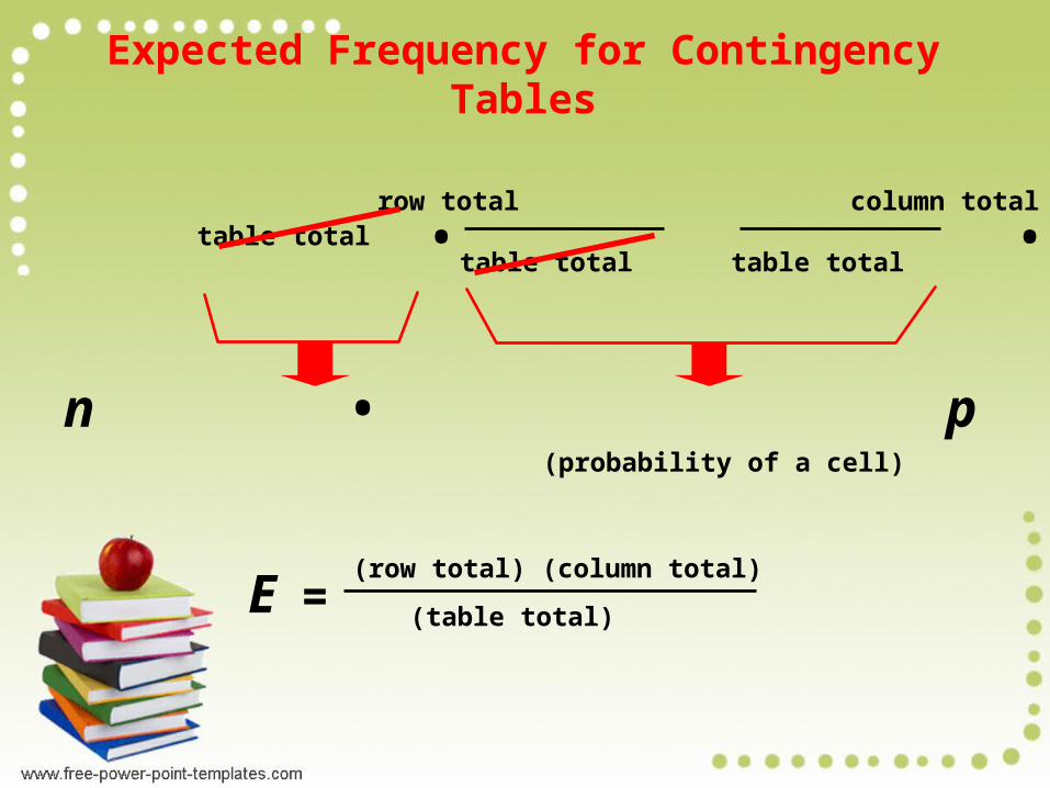
Expected Frequency for Contingency Tables

E = • •table total

row total column total

table totaltable total

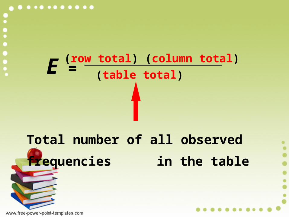
E = (row total) (column total)

(table total)

(probability of a cell)

n • p

(row total) (column total)

(table total)E =

Total number of all observed frequencies

in the table

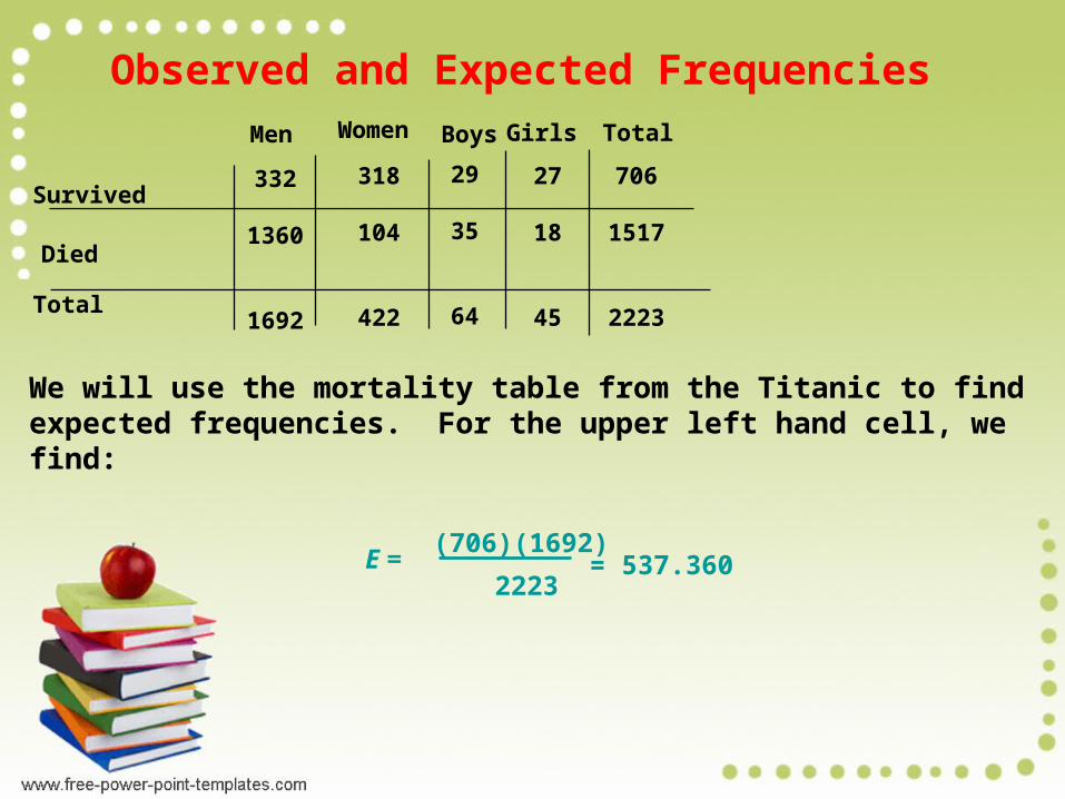
Observed and Expected Frequencies

332

1360

1692

318

104

422

29

35

64

27

18

45

706

1517

2223

Men Women Boys Girls Total

Survived

Died

Total

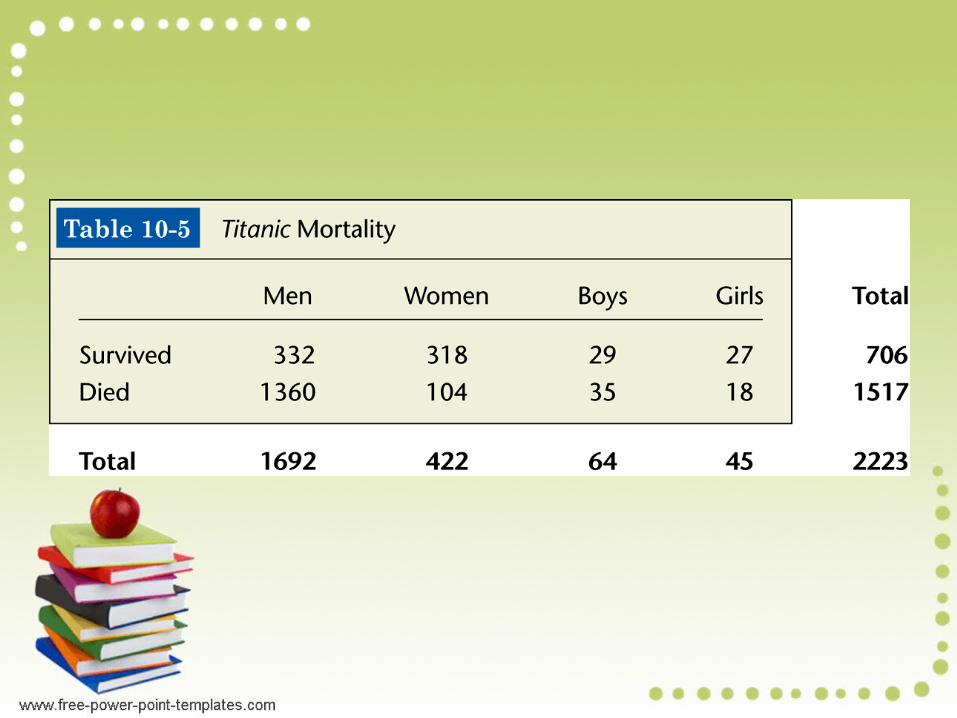
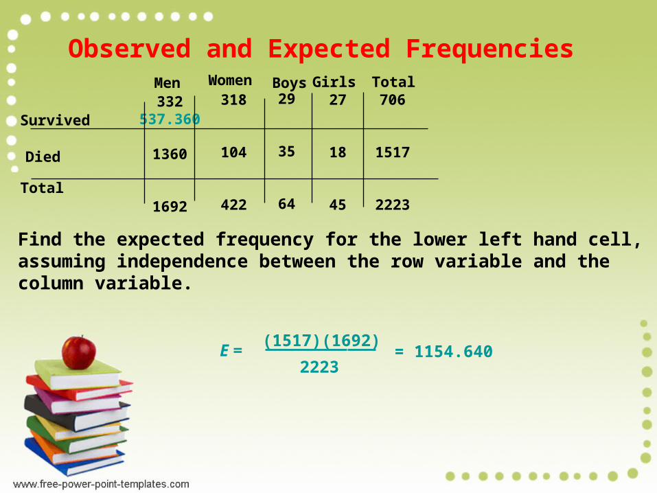
We will use the mortality table from the Titanic to find expected frequencies. For the upper left hand cell, we find:

= 537.360E =(706)(1692)

2223

332537.360

1360

1692

318

104

422

29

35

64

27

18

45

706

1517

2223

Men Women Boys Girls Total

Survived

Died

Total

Find the expected frequency for the lower left hand cell, assuming independence between the row variable and the column variable.

= 1154.640E =

(1517)(1692)

2223

Observed and Expected Frequencies

332537.360

13601154.64

1692

318134.022

104287.978

422

2920.326

3543.674

64

2714.291

1830.709

45

706

1517

2223

Men Women Boys Girls Total

Survived

Died

Total

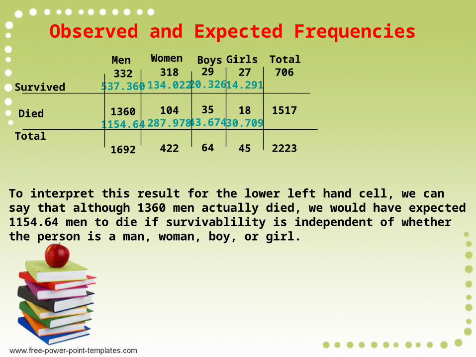
To interpret this result for the lower left hand cell, we can say that although 1360 men actually died, we would have expected 1154.64 men to die if survivablility is independent of whether the person is a man, woman, boy, or girl.

Observed and Expected Frequencies

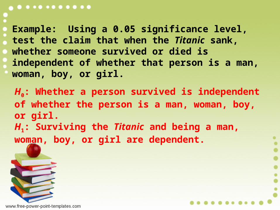
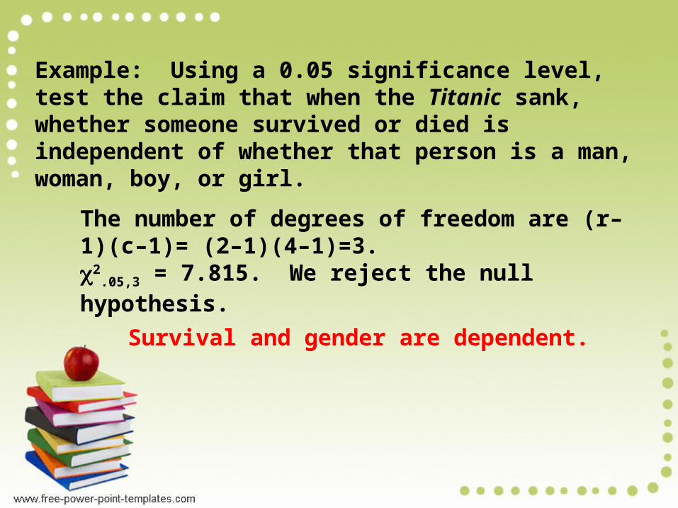
Example: Using a 0.05 significance level, test the claim that when the Titanic sank, whether someone survived or died is independent of whether that person is a man, woman, boy, or girl.

H0: Whether a person survived is independent of whether the person is a man, woman, boy, or girl.H1: Surviving the Titanic and being a man, woman, boy, or girl are dependent.

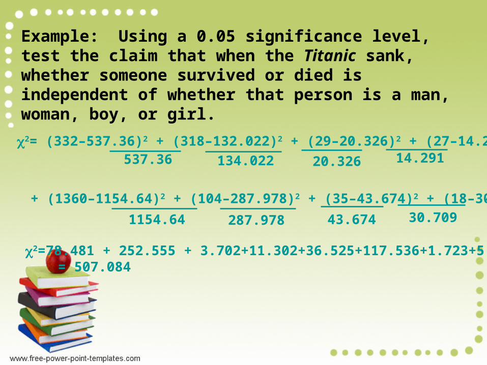
Example: Using a 0.05 significance level, test the claim that when the Titanic sank, whether someone survived or died is independent of whether that person is a man, woman, boy, or girl.

2= (332–537.36)2 + (318–132.022)2 + (29–20.326)2 + (27–14.291)2 537.36 134.022 20.326 14.291

+ (1360–1154.64)2 + (104–287.978)2 + (35–43.674)2 + (18–30.709)2

1154.64 287.978 43.674 30.709

2=78.481 + 252.555 + 3.702+11.302+36.525+117.536+1.723+5.260 = 507.084

Example: Using a 0.05 significance level, test the claim that when the Titanic sank, whether someone survived or died is independent of whether that person is a man, woman, boy, or girl.

The number of degrees of freedom are (r–1)(c–1)= (2–1)(4–1)=3.2

.05,3 = 7.815. We reject the null hypothesis.

Survival and gender are dependent.

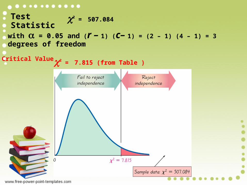
Test Statistic 2 = 507.084

with = 0.05 and (r – 1) (c– 1) = (2 – 1) (4 – 1) = 3 degrees of freedom

Critical Value 2 = 7.815 (from Table )

Example

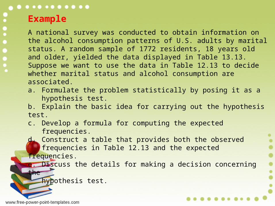
A national survey was conducted to obtain information on the alcohol consumption patterns of U.S. adults by marital status. A random sample of 1772 residents, 18 years old and older, yielded the data displayed in Table 13.13.  Suppose we want to use the data in Table 12.13 to decide whether marital status and alcohol consumption are associated.a. Formulate the problem statistically by posing it as a

hypothesis test.b. Explain the basic idea for carrying out the hypothesis test.c. Develop a formula for computing the expected

frequencies.d. Construct a table that provides both the observed

frequencies in Table 12.13 and the expected frequencies.e. Discuss the details for making a decision concerning the

hypothesis test.

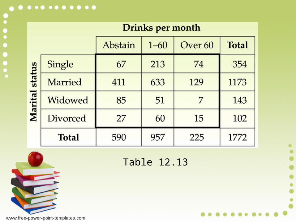
Table 12.13

Solution Example

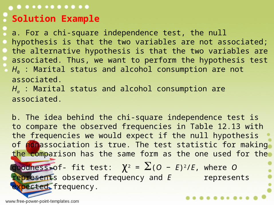
a. For a chi-square independence test, the null hypothesis is that the two variables are not associated; the alternative hypothesis is that the two variables are associated. Thus, we want to perform the hypothesis testH0 : Marital status and alcohol consumption are not associated.Ha : Marital status and alcohol consumption are associated.

b. The idea behind the chi-square independence test is to compare the observed frequencies in Table 12.13 with the frequencies we would expect if the null hypothesis of nonassociation is true. The test statistic for making the comparison has the same form as the one used for the goodness-of- fit test: χ2 = (O − E)2/E, where O represents observed frequency and E

represents expected frequency.

Solution Example

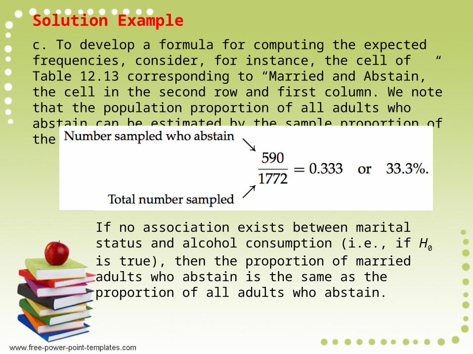
c. To develop a formula for computing the expected frequencies, consider, for instance, the cell of Table 12.13 corresponding to “Married and Abstain,” the cell in the second row and first column. We note that the population proportion of all adults who abstain can be estimated by the sample proportion of the 1772 adults sampled who abstain, that is, by

If no association exists between marital status and alcohol consumption (i.e., if H0 is true), then the proportion of married adults who abstain is the same as the proportion of all adults who abstain.

Solution Example

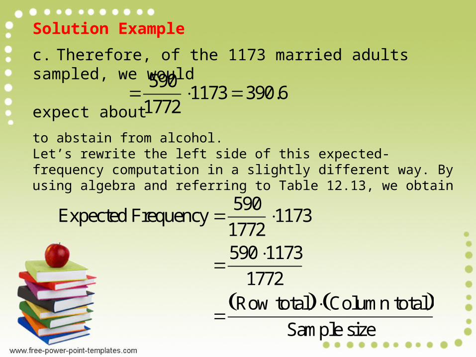
c. Therefore, of the 1173 married adults sampled, we would

expect about

to abstain from alcohol.Let’s rewrite the left side of this expected-frequency computation in a slightly different way. By using algebra and referring to Table 12.13, we obtain

Expected Frequency 590

17721173

5901173

1772

Row total Column total

Sample size

590

17721173390.6

Solution Example

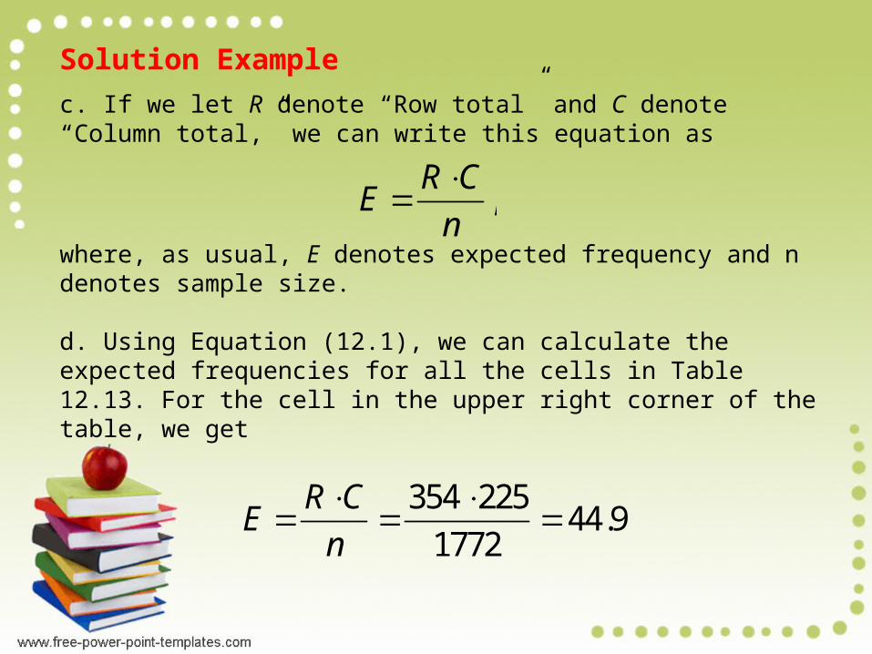
c. If we let R denote “Row total” and C denote “Column total,” we can write this equation as

where, as usual, E denotes expected frequency and n denotes sample size.

d. Using Equation (12.1), we can calculate the expected frequencies for all the cells in Table 12.13. For the cell in the upper right corner of the table, we get

E RCn

,

E RCn

354225

177244.9

Solution Example

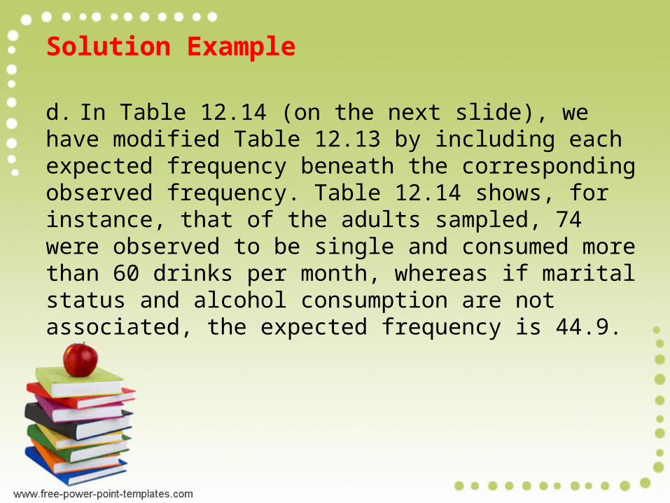
d. In Table 12.14 (on the next slide), we have modified Table 12.13 by including each expected frequency beneath the corresponding observed frequency. Table 12.14 shows, for instance, that of the adults sampled, 74 were observed to be single and consumed more than 60 drinks per month, whereas if marital status and alcohol consumption are not associated, the expected frequency is 44.9.

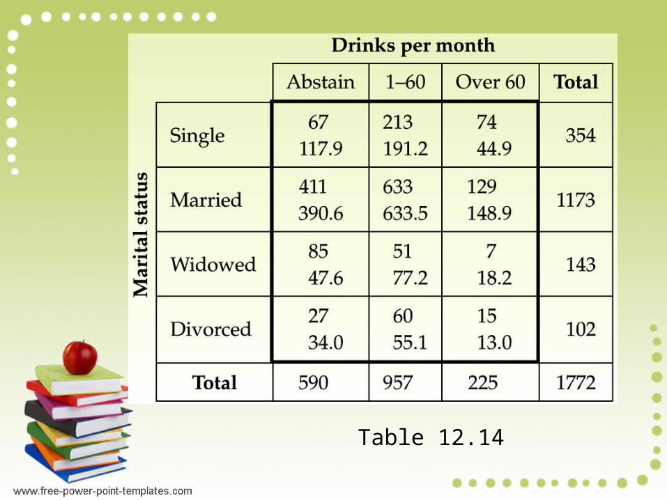
Table 12.14

Solution Example

e. If the null hypothesis of nonassociation is true, the observed and expected frequencies should be approximately equal, which would result

in a relatively small value of the test statistic, χ2= (O − E)2/E.

Consequently, if χ2 is too large, we reject the null hypothesis and conclude that an association exists between marital status and alcohol consumption. From Table 12.14, we find that

χ2= (O − E)2/E = 94.269Can this value be reasonably attributed to sampling error, or is it large enough to indicate that marital status and alcohol consumption are

associated? Before we can answer that question, we must know

the distribution of the χ2-statistic.

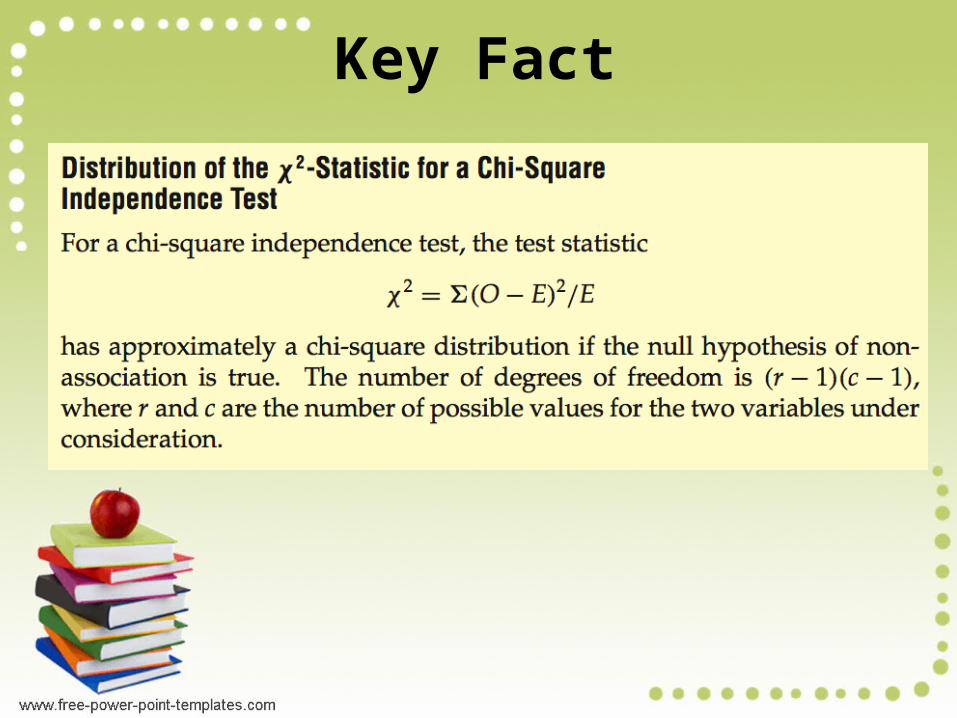
Key Fact

Procedure

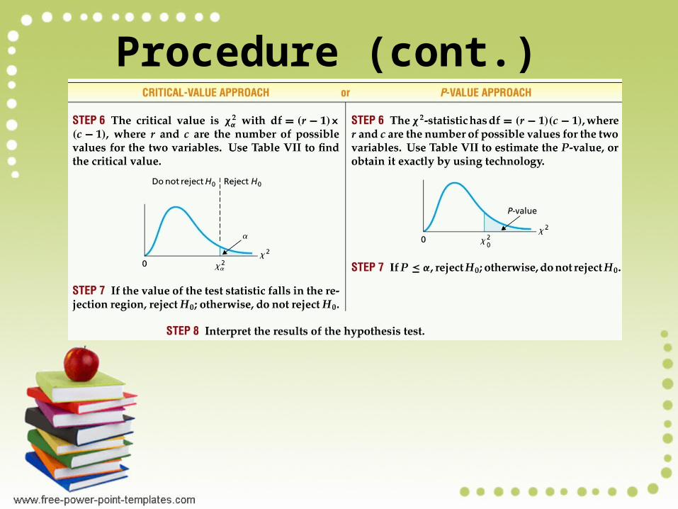
Procedure (cont.)

EXAMPLE • A survey was done by a car

manufacturer concerning a particular make and model. A group of 500 potential customers were asked whether they purchased their current car because of its appearance, its performance rating, or its fixed price (no negotiating). The results, broken down by gender responses, are given on the next slide.

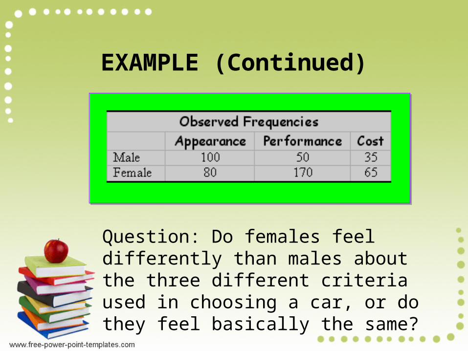
EXAMPLE

(Continued)

Question: Do females feel differently than males about the three different criteria used in choosing a car, or do they feel basically the same?

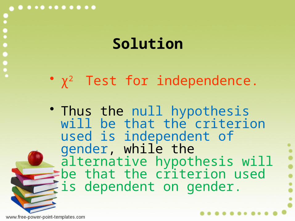
Solution

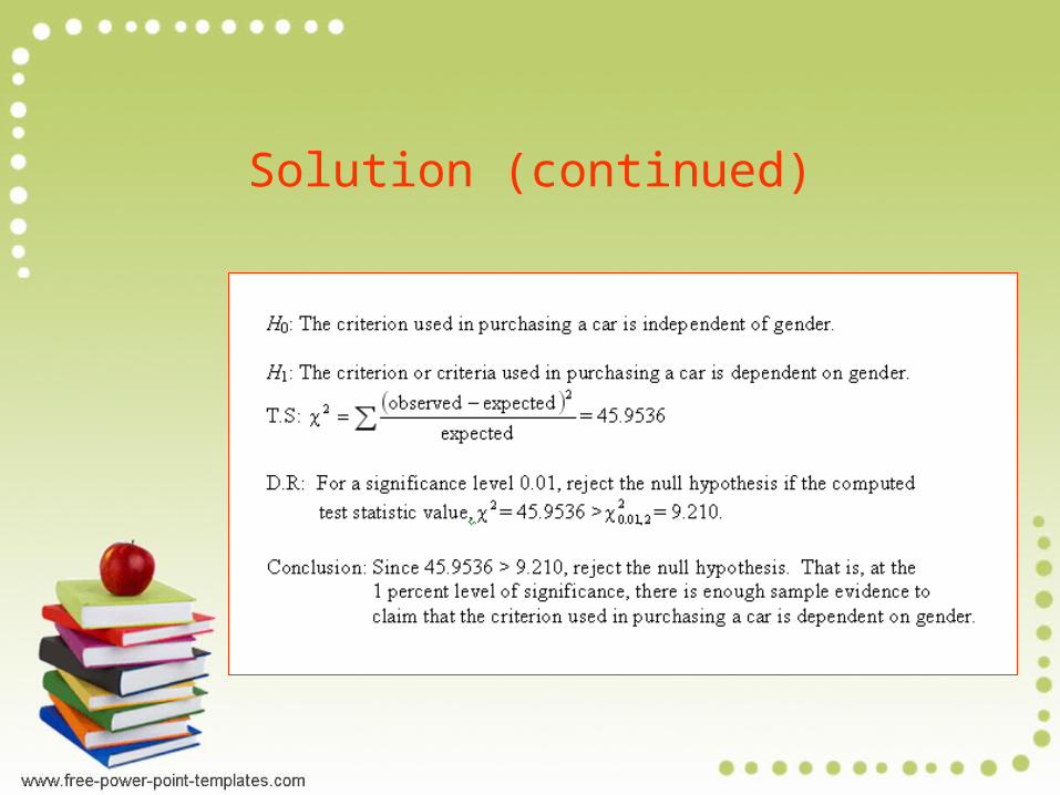
• χ2 Test for independence. • Thus the null hypothesis will be

that the criterion used is independent of gender, while the alternative hypothesis will be that the criterion used is dependent on gender.

Solution (continued)

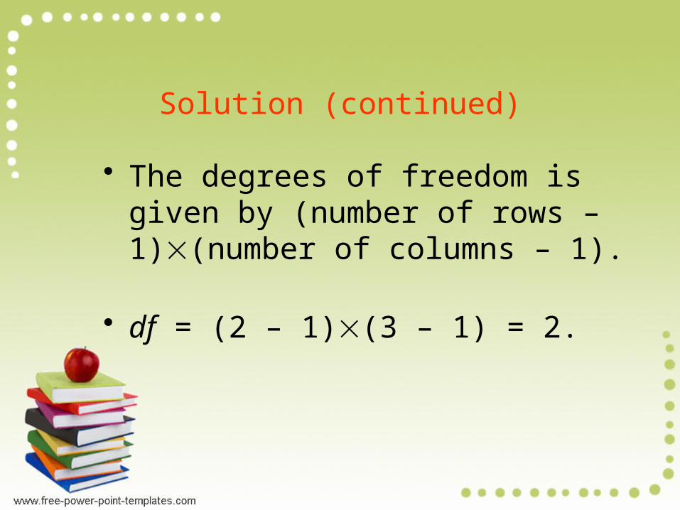
• The degrees of freedom is given by (number of rows – 1)(number of columns – 1).

• df = (2 – 1)(3 – 1) = 2.

Solution (continued)

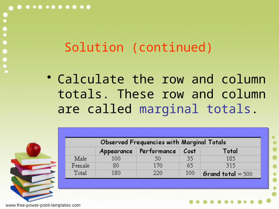
• Calculate the row and column totals. These row and column are called marginal totals.

Solution (continued)

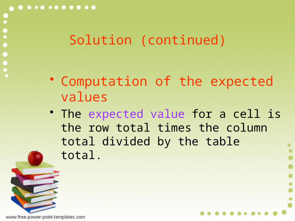
• Computation of the expected values

• The expected value for a cell is the row total times the column total divided by the table total.

Solution (continued)

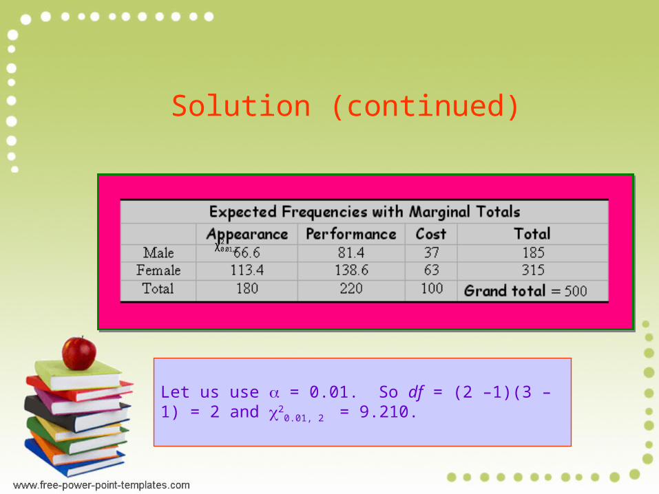
Let us use = 0.01. So df = (2 –1)(3 –1) = 2 and 20.01, 2

= 9.210.

22 ,01.0χ

Solution (continued)

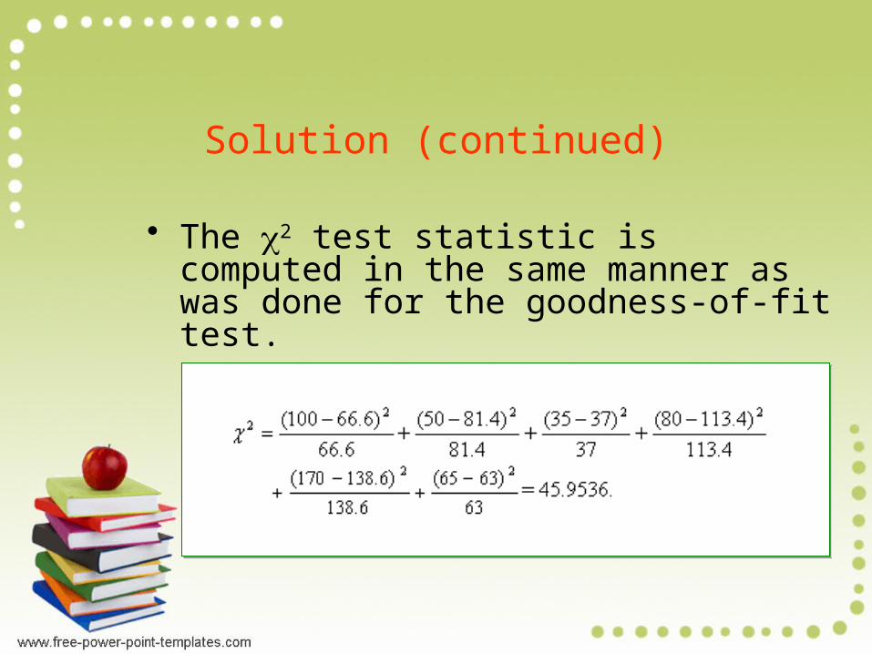
• The 2 test statistic is computed in the same manner as was done for the goodness-of-fit test.

Solution (continued)

Solution (continued)

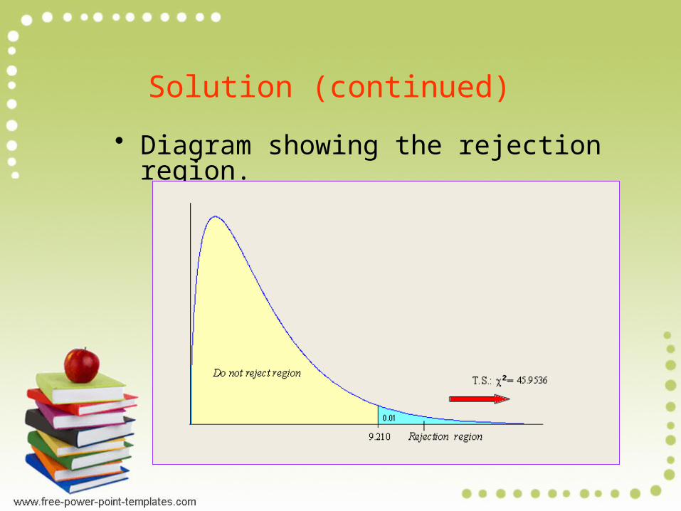
• Diagram showing the rejection region.

Problems

• Review Set 8A – 12, 13 • Review Set 8B – 10,11