Checking the Brain Mapping Hypothesis:

Predicting and Validating BOLD Curves for a Complex Task Using ACT-R

Claus Möbus (claus.moebus@uni-oldenburg.de)

Jan Charles Lenk (jan.lenk@uni-oldenburg.de)

Arno Claassen (arno.claassen@ uni-oldenburg.de) Department of Computing Science, University of Oldenburg

D-26121 Oldenburg, Germany

Jale Özyurt (jale.oezyurt@uni-oldenburg.de)

Christiane M. Thiel (christiane.thiel@uni-oldenburg.de) Department of Psychology, University of Oldenburg

D-26121 Oldenburg, Germany

Abstract

John R. Anderson proposed a correspondence between ACT-R modules and brain regions (Brain Mapping Hypothesis). Using a paradigm requiring rule-based matching of chemical structures (pseudo formulae) with their respective names, we compared ACT-R-generated blood-oxygen-level dependent (BOLD) signal curves with BOLD curves obtained from functional Magnetic Resonance Imaging (fMRI) scans. We found significant correlations between ACT-R generated and human BOLD curves for sensory and motor modules and regions in particular, whereas a lack of significant results was observed for mappings between internal modules and regions. This result was ascribed to the fact that in contrast to Anderson’s studies, our subjects were not urged to follow a single strategy. Instead the task allowed them to construct their personal strategy within a constraint-based strategy space. Accordingly, the mapping hypothesis was tested strategy-specific. As subjects are generally not able to reliably identify their own in a retrospective manner, we used Response-Time (RT) data in combination with a Bayesian Belief Net to identify personal problem solving strategies.

Keywords: ACT-R; BOLD signal prediction, brain-mapping hypothesis

Introduction

The ACT-R architecture (Anderson, 2004) provides a set of

modules with sensory, motor, and internal functions.

Anderson (2007a; Anderson, et al., 2008b) proposes a

neurophysiologic analogy and postulates a mapping

between these modules and brain regions (Table 1). For

instance, the Procedural module is mapped onto the basal

ganglia, while the Declarative module is mapped around the

inferior frontal sulcus. The ACT-R 6.0 implementation

provides a set of tools which directly predict BOLD signals

for these brain regions. Indeed, Anderson has “[..] defined

these regions once and for all and use them over and over

again in predicting different experiments” (2007b).

Several studies were conducted by Anderson et al. in

order to empirically validate the mapping hypothesis. These

included experiments from various domains, like algebraic

problem solving (Danker & Anderson, 2007; Stocco &

Anderson, 2008), associative learning (Anderson et al.,

2008a) or insight problems (Anderson et al., 2009). One

particular feature in common of all these experiments was

the fact that participants had to employ the same problem

solving strategy on all tasks.

The empirical validation of the mapping hypothesis is

among the research goals of our multidisciplinary research

project (see Section Acknowledgements). While also the

effects of affective and informative feedback on learning are

being studied (Özyurt, Rietze, & Thiel, 2008) an

accompanying fMRI study offers us the possibility to

compare BOLD signal predictions generated from strategy-

specific ACT-R models with BOLD signals obtained from

actual fMRI scans.

Table 1: ACT-R module/regions mappings according to

Anderson (2007a) with positions in Talairach coordinate

and dimensions (D, W, H) in voxels

Results of the present study suggest a further refinement

of our modeling methods. In contrast to the experiments

described by Anderson et. al. (2008a; Danker & Anderson,

2007; Stocco & Anderson, 2008), the tasks in our

experimental setting were far more complex; because in

order to solve these tasks, participants were free to choose

their personal strategies. Because different strategies lead to

different predictions of brain region activation, we had to

model these different strategies and identify the chosen

subject-specific strategy without using fMRI data (Möbus &

Lenk, 2009). We would work unduly in favor of the

mapping hypothesis if we would assign subjects to

strategies according to similarity of their BOLD curves with

the strategy-specific ACT-R-BOLD curves.

Module Region X Y Z D W H

Declarative Prefrontal ±40 21 21 5 5 4

Imaginal Parietal ±23 -64 34 5 5 4

Manual Motor ±41 -20 50 5 5 4

Goal ACC ±5 10 38 5 3 4

Procedural Caudate ±15 9 2 4 4 4

Visual Fusiform ±42 -61 -9 5 5 4

Aural Auditory ±46 -22 9 5 5 4

Vocal Motor ±43 -14 33 5 5 4

163

Experiment

All participants were lower-grade schoolchildren with ages

ranging from 11 to 13. The exercises which the children had

to solve came from the domain of the chemical formula

language (Heuer & Parchmann, 2008), which is generally

unknown to children of that age. However, instead of real-

world chemical elements, pseudo-elements (like Pekir or

Nukem) were used to ensure that the children exclusively

applied the rules of the artificial formula language. The

children were asked to answer 80 trials in two sessions

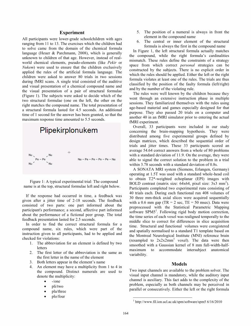
during fMRI scans. A single trial consisted of the auditive

and visual presentation of a chemical compound name and

the visual presentation of a pair of structural formulae

(Figure 1). The subjects were asked to decide which of the

two structural formulae (one on the left, the other on the

right matches the compound name. The total presentation of

a structural formula lasted for 4.5 seconds. An additional

time of 1 second for the answer has been granted, so that the

maximum response time amounted to 5.5 seconds.

Figure 1: A typical experimental trial: The compound

name is at the top, structural formulae left and right below.

If the response had occurred in time, a feedback was

given after a jitter time of 2-18 seconds. The feedback

consisted of two parts: one part informed about the

participant's performance; a second, affective part informed

about the performance of a fictional peer group. The total

feedback presentation lasted for 2.5 seconds.

In order to find the correct structural formula for a

compound name, six rules, which were part of the

instruction given to all participants, had to be applied and

checked for violations:

1. The abbreviation for an element is defined by two

letters

2. The first letter of the abbreviation is the same as

the first letter in the name of the element

3. Both letters appear in the element’s name

4. An element may have a multiplicity from 1 to 4 in

the compound. Distinct numerals are used to

denote the multiplicity:

-/one

pli/two

pla/three

plo/four

5. The position of a numeral is always in front the

element in the compound name

6. The central or inner element of the structural

formula is always the first in the compound name

In Figure 1, the left structural formula actually matches

the compound, while the right formula’s cardinalities

mismatch. These rules define the constraints of a strategy

space from which correct personal strategies can be

constructed by the subjects. There is no explicit order in

which the rules should be applied. Either the left or the right

formula violates at least one of the rules. The trials are thus

classified by the position of the faulty formula (left/right)

and by the number of the violating rule.

The rules were well known by the children because they

went through an extensive instruction phase in multiple

sessions. They familiarized themselves with the rules using

age-based material and games especially designed for that

purpose. They also passed 20 trials on a computer and

another 40 in an fMRI simulator prior to entering the actual

fMRI experiment.

Overall, 33 participants were included in our study

concerning the brain-mapping hypothesis. They were

distributed among five experimental groups defined by

design matrices, which described the sequential order of

trials and jitter times. These 33 participants scored an

average 54.64 correct answers from a whole of 80 problems

with a standard deviation of 11.9. On the average, they were

able to signal the correct solution to the problem in a trial

within 3.78 seconds with a standard deviation of 0.8s.

A SONATA MRI system (Siemens, Erlangen, Germany)

operating at 1.5T was used with a standard whole-head coil

to obtain T2*-weighted echoplanar (EPI) images with

BOLD contrast (matrix size: 64x64, pixel size: 3x3 mm2).

Participants completed two experimental runs consisting of

40 trials each. During each functional run 408 volumes of

30 three mm-thick axial slices were acquired sequentially

with a 0.6 mm gap (TR = 2 sec, TE = 50 msec). Data were

preprocessed with the Statistical Parametric Mapping

software SPM51. Following rigid body motion correction,

the time series of each voxel was realigned temporally to the

middle slice to correct for differences in slice acquisition

time. Structural and functional volumes were coregistered

and spatially normalised to a standard T1 template based on

the Montreal Neurological Institute (MNI) reference brain

(resampled to 2x2x2mm3 voxel). The data were then

smoothed with a Gaussian kernel of 8 mm full-width-half-

maximum to accommodate intersubject anatomical

variability.

Models

Two input channels are available to the problem solver. The

visual input channel is mandatory, while the auditory input

channel is auxiliary. This fact adds to the complexity of the

problem, especially as both channels may be perceived in

parallel or consecutively. Either the left or the right formula

1 http://www.fil.ion.ucl.ac.uk/spm/software/spm5 6/16/2010

164

or both have to be evaluated visually. This results in a

variability of conceivable strategies, which differ in

efficiency as well as module activation. A set of basic tasks

is derived from the rules. These tasks are shared by all

strategies, though not necessarily in the order presented

here:

1. Visually and/or auditorially perceive and encode

the different parts of the compound name

(mandatory for any successful strategy)

2. Count the outer elements of a structural formula

and compare them with the second numeral in the

compound name

3. Count the inner elements of a structural formula

and compare them with the first numeral

4. Compare the inner element with the first element

of the compound name

5. Compare the outer element with the second

element of the compound name

6. Indicate the correct formula

Tasks 2-5 may be applied to both formulae, or, more

efficiently, to either the left or the right formula. It should be

noted that some concurrency can take place if the compound

name is encoded using only auditory input. Tasks 4 and 5

may be split into two different tasks as the abbreviation of

an element always consists of two letters. Since the first

letter is easier to compare with the name, it may be more

appropriate to prioritize the first comparison and leave the

second letter for later. A second open question which is not

reflected within the above list of tasks is the position of the

retrieval for the numerals. It can take place very early when

encoding the compound name, but there is also the

possibility to retrieve the numeral later on between the

counting and comparison stages.

A strategy is defined by the order of task processing and

the formulae Tasks 2-5 are applied to. While all the

strategies share the same basic set of tasks, they all perform

differently on each trial. Some trials may only be solved by

counting the elements as in Figure 1, others by name-

element comparisons, still others by both. A strategy shows

higher performance (shorter response time) if it concentrates

on a single structural formula to decide whether it matches

or not. Each trial class (the violated rule and location of the

violating formula) may have an impact on the performance

of the strategy.

Several, though so far not all possible, strategies were

modeled, at first on an abstract layer as UML activity

diagrams, and subsequently within the ACT-R environment

as a set of production rules. As only expert participants were

modeled, all modeled strategies find the correct answer but

with a large variation in performance. So far, four different

strategies, S1 to S4, have been modeled (Table 2). They

differ in that they either process the structural formula and

the compound name simultaneously using the different

input channels, or by processing the compound name first

and then proceed to the structural formulae. Thus they either

process the trial single- or multithreaded, or single-formula

or both formulae.

Table 2: Characteristics of strategies/models

Multi-Thread Single-Thread

Single Formula S1 S3

Both Formulae S2 S4

Apart from these single- vs. multi-tasking and single vs.

both formulae considerations, even more design options are

available to the modeler yet. For instance, the exact time

when certain tests are carried out may be varied. Thus, the

model could compare the element's abbreviations with their

respective names before comparing the cardinalities. Also,

the costly checking of the second letter of the abbreviation

may be postponed by the strategy in order to save time. A

heuristic approach could leave the second letter out of

consideration completely.

The models perform quite differently on the various trials,

which is reflected in the ACT-R module traces. This affects

the BOLD prediction. Any realization of Task 1, perceiving

and encoding the compound name, would surely engage

ACT-R's Visual or Aural module, if not both, and the

Imaginal module. Tasks 2 and 3, which encompass

encoding and counting the structural formulae, would

involve the Imaginal, the Visual and the Declarative

module. Tasks 4 and 5 would also require at least the

Imaginal module, but it could involve the Visual module if

the second letter of the symbol has to be checked for

occurrence in the compound name. As Tasks 2-5 can be

arranged in any arbitrary order, or even be split into

subtasks which could run in parallel, quite different patterns

of module activation would emerge. This implies that even

models which produce similar behaviors may predict

distinct BOLD signals, if the productions involved activate

different modules.

Data Analysis

It is doubtful whether the participants are able to remember

their problem solving strategy for each trial. It is also

possible that they applied varying strategies to trials. The

choice of strategy may be related to the trial class. However,

we assume that the participants already settled for a single

strategy after the extensive instruction and training phases.

In order to determine which of our models is suitable to

explain the performance of the actual strategy used by the

participant, we devised a Bayesian Classifier with a

Bayesian Belief Network (BBN) (Jensen, 2007) as

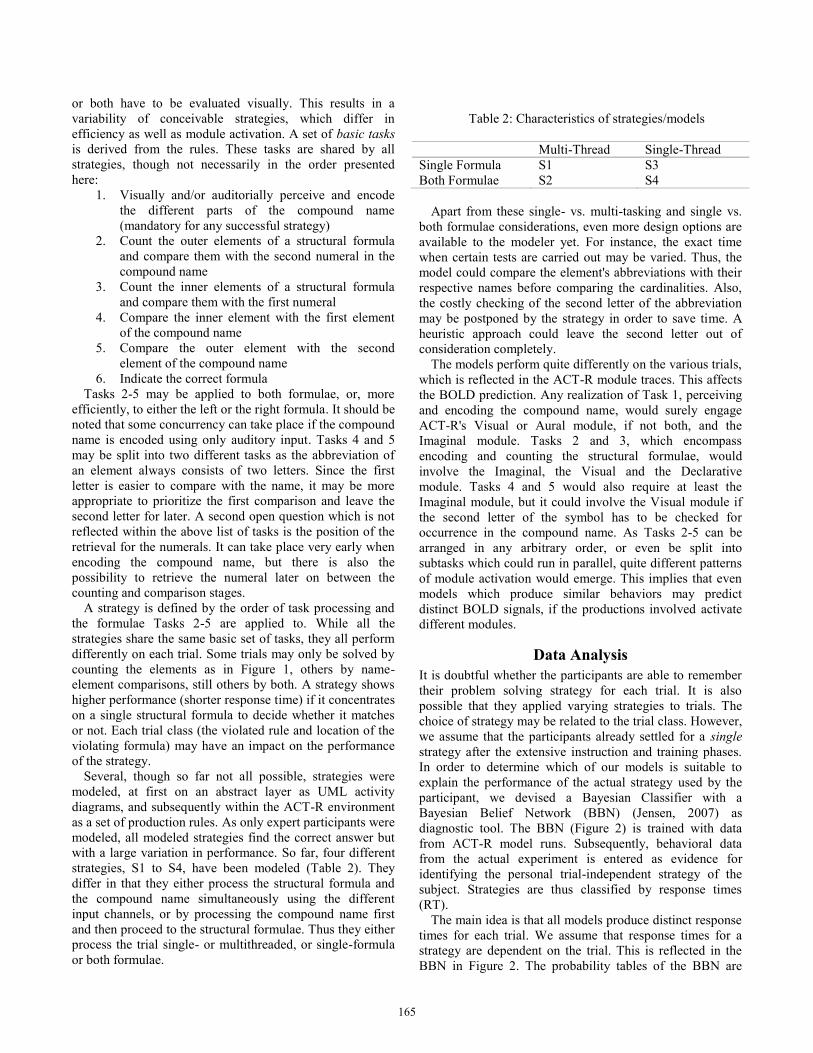
diagnostic tool. The BBN (Figure 2) is trained with data

from ACT-R model runs. Subsequently, behavioral data

from the actual experiment is entered as evidence for

identifying the personal trial-independent strategy of the

subject. Strategies are thus classified by response times

(RT).

The main idea is that all models produce distinct response

times for each trial. We assume that response times for a

strategy are dependent on the trial. This is reflected in the

BBN in Figure 2. The probability tables of the BBN are

165

P1 P2 P3

fMRI scans

ACT-R module activations

Strategy Classifier

Individual BOLD curves in selected ROI

Provides weights for BOLD curves aggregation for a strategy S

Predictionaccording toBrain Mapping Hypothesis

Co

rrel

atio

nte

st

Map

pin

g

1 3 5 7 9 11 13 15

BO

LD a

ctiv

atio

n

Time Aural S3 left

T13

T14 T15

590

600

610

620

630

640

1 2 3 4 5 6 7 8 9 10 11 12 13 14 15

Gra

yval

ues

Time

Avg

P1

P2

P3

P4

P5

P6

P7

T1 T14 T15

being learned by running all of the strategy-specific ACT-R

models to generate cases. This results in a data matrix

whose columns correspond to the nodes from the BBN and

whose rows correspond to trials. During model runs, the

default values of ACT-R’s parameters were used.

Figure 2: BBN for strategy classification

The trial is entered as evidence into the “Trial”, “Matrix”,

and “Session” nodes. The response time of the participant is

entered as evidence into the “RT” node. It is then possible to

infer on the strategy most likely used by the participant in

the “Strategy” node. In Figure 2, the trial in question is the

14th

trial from the second session of the experimental group

defined by design matrix 1407. In this particular case, for

participant with a response time between 4 and 4.5 seconds,

S2 and S3 are equally probable.

The collected fMRI data is analyzed by using the Regions

of Interest (ROI) approach (Jäncke, 2005). The regions are

specified by the module positions and dimensions given by

Anderson’s Brain Mapping Hypothesis in Table 1. The

Talairach coordinates were transformed into MNI

coordinates. The raw values of each voxel lying in the ROI

are extracted from the images and averaged per region,

resulting in an activation timeline for each person and

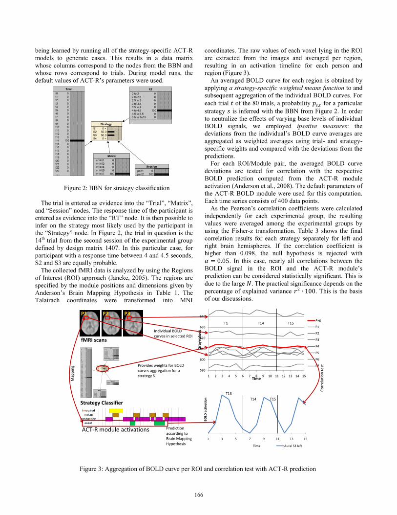
region (Figure 3).

An averaged BOLD curve for each region is obtained by

applying a strategy-specific weighted means function to and

subsequent aggregation of the individual BOLD curves. For

each trial 𝑡 of the 80 trials, a probability 𝑝𝑠,𝑡 for a particular

strategy 𝑠 is inferred with the BBN from Figure 2. In order

to neutralize the effects of varying base levels of individual

BOLD signals, we employed ipsative measures: the

deviations from the individual’s BOLD curve averages are

aggregated as weighted averages using trial- and strategy-

specific weights and compared with the deviations from the

predictions.

For each ROI/Module pair, the averaged BOLD curve

deviations are tested for correlation with the respective

BOLD prediction computed from the ACT-R module

activation (Anderson et al., 2008). The default parameters of

the ACT-R BOLD module were used for this computation.

Each time series consists of 400 data points.

As the Pearson’s correlation coefficients were calculated

independently for each experimental group, the resulting

values were averaged among the experimental groups by

using the Fisher-z transformation. Table 3 shows the final

correlation results for each strategy separately for left and

right brain hemispheres. If the correlation coefficient is

higher than 0.098, the null hypothesis is rejected with

𝛼 = 0.05. In this case, nearly all correlations between the

BOLD signal in the ROI and the ACT-R module’s

prediction can be considered statistically significant. This is

due to the large 𝑁. The practical significance depends on the

percentage of explained variance 𝑟2 ∙ 100. This is the basis

of our discussions.

Figure 3: Aggregation of BOLD curve per ROI and correlation test with ACT-R prediction

166

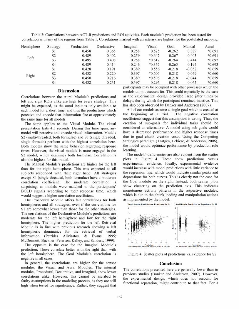
Table 3: Correlations between ACT-R predictions and ROI activities. Each module’s prediction has been tested for

correlation with any of the regions from Table 1. Correlations marked with an asterisk are highest for the postulated mapping

Discussion

Correlations between the Aural Module’s predictions and

left and right ROIs alike are high for every strategy. This

might be expected, as the aural input is only available to

each model for a short time, and thus the productions which

perceive and encode that information fire at approximately

the same time for all models.

The same applies to the Visual Module. The visual

presentation lasts 4.5 seconds. During this time span, any

model will perceive and encode visual information. Models

S2 (multi-threaded, both formulae) and S3 (single threaded,

single formula) perform with the highest correlation here.

Both models show the same behavior regarding response

times. However, the visual module is more engaged in the

S2 model, which examines both formulae. Correlation is

also the highest for this model.

The Manual Module’s predictions are higher for the left

than for the right hemisphere. This was expected as all

subjects responded with their right hand. All strategies

except S4 (single-threaded, both formulae) have a moderate

correlation coefficient. The moderate correlation is

surprising, as models were matched to the participants’

BOLD signals according to their response time, which

would suggest a higher correlation coefficient.

The Procedural Module offers fair correlations for both

hemispheres and all strategies, even if the correlations for

S1 are somewhat lower than those for the other strategies.

The correlations of the Declarative Module’s predictions are

moderate for the left hemisphere and low for the right

hemisphere. The higher prediction for the left Retrieval

Module is in line with previous research showing a left

hemispheric dominance for the retrieval of verbal

information (Petrides Alivisatos, & Evans, 1995;

McDermott, Buckner, Petersen, Kelley, and Sanders, 1999).

The opposite is the case for the Imaginal Module’s

prediction: These correlate better with the right than with

the left hemisphere. The Goal Module’s correlation is

negative in all cases.

In general, the correlations are higher for the sensor

modules, the Visual and Aural Modules. The internal

modules, Procedural, Declarative, and Imaginal, show lower

correlations alike. However, this cannot be ascribed to

faulty assumptions in the modeling process, as they are still

high when tested for significance. Rather, they suggest that

participants may be occupied with other processes which the

models do not account for. This could especially be the case

as the experimental design provided large jitter times or

delays, during which the participant remained inactive. This

has also been observed by Danker and Anderson (2007).

All of our models assume a single goal which is created at

the beginning of a trial. The negative correlation

coefficients suggest that this assumption is wrong. Thus, the

creation of sub-goals for individual tasks should be

considered an alternative. A model using sub-goals would

have a decreased performance and higher response times

due to goal chunk creation costs. Using the Competing

Strategies paradigm (Taatgen, Lebiere, & Anderson, 2006),

the model would optimize performance by production rule

learning.

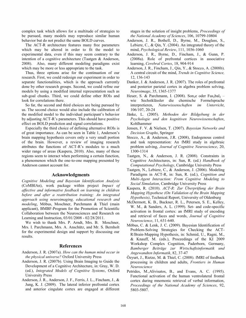
The models’ deficiencies are also evident from the scatter

plots in Figure 4. These show predictions versus

experimental evidence. Ideally, experimental evidence

would increase with model predictions with little variance to

the regression line, which would indicate similar peaks and

depressions for both curves. This is clearly not the case for

the Goal module on the right. Instead, both scatter plots

show clustering on the prediction axis. This indicates

monotonous activity patterns in the respective modules,

which is due to the chunk loading and manipulation actions

as implemented by the model.

Figure 4: Scatter plots of predictions vs. evidence for S2

Conclusion

The correlations presented here are generally lower than in

previous studies (Danker and Anderson, 2007). However,

the experimental design, which does not account for

functional separation, might contribute to that fact. For a

Hemisphere Strategy Production Declarative Imaginal Visual Goal Manual Aural

Left

S1 0.458 0.365 0.258 0.525 -0.262 0.389 *0.691

S2 0.489 0.402 0.259 *0.647 -0.267 0.403 *0.691

S3 0.495 0.408 0.258 *0.617 -0.264 0.414 *0.692

S4 0.489 0.414 0.246 *0.367 -0.265 0.194 *0.693

Right

S1 0.428 0.191 0.389 0.556 -0.218 -0.052 *0.659

S2 0.438 0.220 0.397 *0.606 -0.218 -0.049 *0.660

S3 0.450 0.216 0.389 *0.596 -0.218 -0.044 *0.659

S4 0.432 0.231 0.397 0.295 -0.218 -0.065 *0.660

167

complex task which allows for a multitude of strategies to

be pursued, many models may reproduce similar human

behavior but do not predict the same BOLD curves.

The ACT-R architecture features many free parameters

which may be altered in order to fit the model to

experimental data, even if this may seem contrary to the

intention of a cognitive architecture (Taatgen & Anderson,

2008). Also, many different modeling paradigms exist

which may be more or less appropriate to the task.

Thus, three options arise for the continuation of our

research. First, we could redesign our experiment in order to

separate functionalities, which is the approach currently

done by other research groups. Second, we could refine our

models by using a modified internal representation such as

sub-goal chunks. Third, we could define other ROIs and

look for correlations there.

So far, the second and third choices are being pursued by

us. The second choice would also include the calibration of

the modified model to the individual participant’s behavior

by adjusting ACT-R’s parameters. This should have positive

effect on BOLD prediction and signal correlations.

Especially the third choice of defining alternative ROIs is

of great importance. As can be seen in Table 1, Anderson’s

brain mapping hypothesis covers only a very small portion

of the brain. However, a review of imaging research

attributes the functions of ACT-R’s modules to a much

wider range of areas (Kaspera, 2010). Also, many of these

regions seem to interact when performing a certain function,

a phenomenon which the one-to-one mapping presented by

Anderson cannot account for.

Acknowledgments

Cognitive Modeling and Bayesian Identification Analysis

(CoMBIAn), work package within project Impact of

affective and informative feedback on learning in children

before and after a reattribution training: An integrated

approach using neuroimaging, educational research and

modeling, Möbus, Moschner, Parchmann & Thiel (main

applicant), BMBF-Program for the Promotion of Scientific

Collaboration between the Neurosciences and Research on

Learning and Instruction, 03/01/2008 - 02/28/2011.

We wish to thank Mrs. P. Arndt, Mrs. B. Moschner,

Mrs. I. Parchmann, Mrs. A. Anschütz, and Mr. S. Bernholt

for the experimental design and support by discussing our

results.

References

Anderson, J. R. (2007a). How can the human mind occur in

the physical universe? Oxford University Press

Anderson, J. R. (2007b). Using Brain Imaging to Guide the

Development of a Cognitive Architecture, in: Gray, W. D.

(ed.), Integrated Models of Cognitive Systems, Oxford

University Press

Anderson, J. R., Anderson, J. F., Ferris, J. L., Fincham, J., &

Jung, K. J. (2009). The lateral inferior prefrontal cortex

and anterior cingulate cortex are engaged at different

stages in the solution of insight problems, Proceedings of

the National Academy of Sciences, 106, 10799-10804

Anderson, J. R., Bothell, D., Byrne, M., Douglass, S.,

Lebiere, C., & Qin, Y. (2004). An integrated theory of the

mind, Psychological Review, 111, 1036-1060

Anderson, J. R., Byrne, D., Fincham, J., & Gunn, P.

(2008a). Role of prefrontal cortices in associative

learning, Cerebral Cortex, 18, 904-914

Anderson, J. R., Fincham, J., Qin, Y., & Stocco, A. (2008b).

A central circuit of the mind, Trends in Cognitive Science,

12, 136-143

Danker, J. & Anderson, J. R. (2007). The roles of prefrontal

and posterior parietal cortex in algebra problem solving,

Neuroimage, 35, 1365-1377

Heuer, S. & Parchmann, I. (2008). Son2e oder Fus2bal2 –

wie Sechstklässler die chemische Formelsprache

interpretieren, Naturwissenschaften im Unterricht,

106/107, 20-24

Jänke, L. (2005). Methoden der Bildgebung in der

Psychologie und den kognitiven Neurowissenschaften,

Kohlhammer

Jensen, F. V. & Nielsen, T. (2007). Bayesian Networks and

Decision Graphs, Springer

Stocco, A., & Anderson, J.R. (2008), Endogenous control

and task representation: An fMRI study in algebraic

problem solving, Journal of Cognitive Neuroscience, 20,

1300-1314

Taatgen, N., & Anderson, J. R. (2008). Constraints in

Cognitive Architectures, in: Sun, R. (ed.) Handbook of

Computational Psychology, Cambridge University Press

Taatgen, N., Lebiere, C., & Anderson, J. (2006). Modeling

Paradigms in ACT-R, in: Sun, R. (ed.), Cognition and

Multi-Agent Interaction: From Cognitive Modeling to

Social Simulation, Cambridge University Press

Kaspera, R. (2010). ACT-R: Zur Überprüfung der Brain

Mapping Hypothese (On Validation of the Brain Mapping

Hypothesis), Technical Report, University of Oldenburg

McDermott, K. B., Buckner, R. L., Petersen, S. E., Kelley,

W. M., & Sanders, A. L. (1999). Set- and code-specific

activation in frontal cortex: an fMRI study of encoding

and retrieval of faces and words, Journal of Cognitive

Neuroscience, 11, 631-640.

Möbus, C. & Lenk, J. C. (2009). Bayesian Identification of

Problem-Solving Strategies for Checking the ACT-

R/Brain-Mapping Hypothesis, in: Schmid, U., Ragni, M.,

& Knauff, M. (eds.), Proceedings of the KI 2009

Workshop Complex Cognition, Paderborn, Germany,

Bamberger Beiträge zur Wirtschaftsinformatik und

Angewandten Informatik, 82, 37-47

Özyurt, J., Rietze, M. & Thiel, C. (2008). fMRI of feedback

processing in children and adults, Frontiers in Human

Neuroscience

Petrides, M.,Alivisatos, B., and Evans, A. C. (1995).

Functional activation of the human ventrolateral frontal

cortex during mnemonic retrieval of verbal information,

Proceedings of the National Academy of Sciences, 92,

5803-5807.

168