characterization of the performance of mineral oil based … · · 2002-08-29characterization of...
TRANSCRIPT

Characterization of the performance of mineral oil based quenchants using CHTE Quench Probe System
By
Shuhui Ma
A Thesis
Submitted to the Faculty
Of the
WORCESTER POLYTECHNIC INSTITUTE
In partial fulfillment of the requirements for the
Degree of Master
In
Materials Science and Engineering
By
____________________
June 27, 2002
APPROVED: _____________________________________ Richard D. Sisson Jr. Advisor, Professor of Mechanical Engineering Materials Science and Engineering Program Head

i
ABSTRACT
The performance of a series of mineral oil based quenchants has been investigated
using the CHTE Quench Probe System and probe tips of 4140 steel to determine the cooling
rate, heat transfer coefficient, Hardening Power (HP) and Tamura’s V indices in terms of the
physical properties of quenchants; e.g. viscosity and oil start temperature. The Quench Factor,
Q, was also calculated in terms of the hardness of the quenched parts. The lumped parameter
approximation was used to calculate the heat transfer coefficient as a function of temperature
during quenching. The results revealed that the maximum cooling rate increases with decrease
in quenchant viscosity. As viscosity increases, Tamura’s V is nearly constant, while the HP
decreases. For the selected oils, cooling ability of quenching oil increases with the increase in
oil operating temperature, reaches a maximum and then decreases. The heat transfer
coefficient increases with the increase in hardening power and maximum cooling rate. As the
viscosity increases, the quench factor increases, which indicates the cooling ability of the oil
decreases since the higher quench factor means the lower cooling ability of the oil. The
hardness decreases with the increase in quench factor.
Also the effect of surface oxides during quenching in commercial oils is studied. It was
found that for 4140 steel probes the formation of oxide in air increases the cooling rate and
heat transfer coefficient, the cooling rate curve of 4140 steel probe heated in argon shows clear
Leidenfrost temperature, the oxide layer may require a significant thickness to cause the
decrease in heat transfer coefficient. For 304 stainless steel probes the cooling rate and heat
transfer coefficient are quite similar in air and in argon.

ii
Acknowledgements
First I would like to thank Prof. Richard D. Sisson, Jr. for his support and assistance as
well as the Center for Heat Treating Excellence of the Metal Processing Institute at Worcester
Polytechnic Institute. Also, I want to give my thanks to Dr. Maniruzzaman Mohammed for his
help and creative ideas and to Juan Chaves for helping me start my research. My sincere
thanks go to Torbjorn Bergstrom for his help, encouragement and assistance in measuring the
roughness of the samples in my test.
I want to thank Rita Shilansky for the constant assistance that made this work possible.
My thanks go to Celine McGee, who helped me to carry out some experiments, Olivier Prevot
for helping me out with some excel problems and Marco Fontecchio for his ideas.
Furthermore, I must also acknowledge the patience and assistance of Jim Johnston,
Todd Billings and Stephen Derosier for making the samples.
My sincere gratitude is given to my parents, my sisters and brother for their continuous
encouragement, care and infinite love.

iii
Table of Contents
ABSTRACT......................................................................................................................... i
Acknowledgements............................................................................................................. ii
Table of Contents............................................................................................................... iii
List of Figures ..................................................................................................................... v
List of Tables ................................................................................................................... viii
1. Introduction................................................................................................................. 2
2. Literature Review........................................................................................................ 4
2.1 Quenching and Its Stages.................................................................................... 4
2.1.1 Film boiling phase........................................................................................... 6
2.1.2 Nucleate boiling phase.................................................................................... 6
2.1.3 Convection stage............................................................................................. 7
2.2 Quenchant Chemistry.......................................................................................... 8
2.2.1 Mineral oils ..................................................................................................... 8
2.2.2 Vegetable oils................................................................................................ 12
2.3 Quenchant Characterization.............................................................................. 14
2.4 Quenching probes ............................................................................................. 19
2.4.1 General Motors (GM) quenchometer............................................................ 19
2.4.2 Grossmann Probe .......................................................................................... 21
2.4.3 IVF probe ...................................................................................................... 21
2.4.4 The Drayton Probe........................................................................................ 23
2.4.5 Nanigian-Liscic Probe .................................................................................. 24
2.4.6 Tamura’s Probes ........................................................................................... 25
2.5 Cooling curve analysis...................................................................................... 26
2.5.1 Data Acquisition and Cooling Curve Analysis............................................. 26
2.5.2 Interpretation of cooling curves .................................................................... 28
2.6 Metallurgy of 4140 Steel and 304 Stainless Steel ............................................ 30
2.6.1 Characteristics and TTT diagram of 4140 steel............................................ 30
2.6.2 Characteristics of 304 stainless steel............................................................. 33

iv
2.6.3 Theoretical understanding of heat transfer ................................................... 34
2.6.4 Calculation of heat transfer coefficient......................................................... 40
2.6.5 Thermoconductivity of 4140 steel and 304 stainless steel............................ 43
2.6.6 Specific Heat of 4140 steel and 304 stainless steel....................................... 45
2.7 Quenching Performance Indices ....................................................................... 47
2.7.1 Tamura V value............................................................................................ 48
2.7.2 Hardening Power (HP) by IVF ..................................................................... 48
2.7.3 Quench Factor Analysis................................................................................ 51
3. Characterization of the performance of mineral oil based quenchants using CHTE Quench
Probe System .................................................................................................................... 56
I Introduction ................................................................................................................ 57
II Experimental Procedure ............................................................................................ 59
III Experimental Results and Discussion...................................................................... 61
IV Summary.................................................................................................................. 75
4. The Effects of surface oxides on the quenching performance of 4140 steel in commercial
mineral oils 77
I Introduction ................................................................................................................ 78
II Experimental Procedure ............................................................................................ 80
III Experimental Results and Discussion...................................................................... 83
(A) Repeatability tests............................................................................................... 83
(B) Comparison of cooling rate curves ..................................................................... 90
(C) Comparison of heat transfer coefficients............................................................ 96
(D) Theoretical calculation ..................................................................................... 100
IV Summary................................................................................................................ 104
References................................................................................................................... 105

v
List of Figures Fig 2.1 Cooling mechanism [5]
Fig 2.2 The three cooling stages in quenching [3].
Fig 2.3 Gas chromatogram of the wolfson reference quench oil [5]
Fig 2.4 Expected hydrocarbons in a typical crude oil fraction [5]
Fig 2. 5 Cooling rate curves of various quench oils at 60oC [5]
Fig 2.6 Vegetable oil triglyceride structure [13]
Fig 2.7 Transformation diagram of low- alloy steel with cooling curves for various quenching media [5]
Fig 2. 8 GM quenchometer and principle of operation [5]
Fig 2.9 SAE 5145 Steel Probe used by Grossmann [27]
Fig 2.10 IVF test probe and handle [28]
Fig 2.11 Drayton probe and the portable quenching system
Fig 2.12 Schematic of Liscic-NANMAC probe--TGQAS Temperature Gradient Quenching Analysis
System by Prof. Bozidar Liscic [1]
Fig 2. 13 JIS silver probe [5]
Fig 2.14 various representations of cooling curve data [5]
Fig 2.15 CCT diagram for a spring steel (50M7) with superimposed cooling curves [5]
Fig 2. 16 TTT diagrams of AISI 4140
Fig 2. 17 Cross sections of Fe-Cr-Ni ternary diagram [39]
Fig 2. 18 Thermal conductivity of 4140 steels and 304 stainless steels [39] [41] [32]
Fig 2. 19 Specific Heat of 4140 steels and 304 stainless steels [36] [1, 39, 42, 43]
Fig 2. 20 Specific heat of austenitic iron and 4140 as a function of temperature [36, 42]
Fig 2. 21 Key parameters for IVF hardening power equation [1]
Fig 2. 22 Oils ranked by hardening power. Calculated values of hardening power HP, matched to a

vi
straight line for the quenching oils [53]
Fig 2. 23 Schematic illustrations on plot of CT function to calculate the Quench Factor
Fig 3- 1CHTE Quench Probe System
Fig 3- 2CHTE probe-coupling-connecting rod assembly
Fig 3- 3 typical cooling rate curves of CHTE 4140 steel probe in different mineral oils
Fig 3- 4 Cooling rates of CHTE 4140 steel probe at 800,700,600,550,500 and 400oC as a function of
viscosity
Fig 3- 5 the maximum cooling rate as a function of viscosity
Fig 3-6 Cooling curves of CHTE probe in Houghton Martemp355 used quenching oil show excellent
repeatability of the cooling rate
Fig 3-7 Cooling rate curves of CHTE probe in Houghton T7A mineral oil
Fig 3-8 Cooling rate of CHTE probe in Houghton Mar-temp 355
Fig 3-9 Cooling rate of CHTE probe in Burgdorf HR88A mineral oil
Fig 3-10 Cooing rate of CHTE probe in Burgdorf W72 mineral oil
Fig 3-11 Cooing rate of CHTE probe in Burgdorf Durixol V35 mineral oil
Fig 3-12 Cooing rate of CHTE probe in Burgdorf Durixol W25 mineral oil
Fig 3-14 Cooling rate curves of CHTE 4140 quenched in Burgdorf HR88A at different temperatures
Fig 3-15 Cooling curves of CHTE 4140 probes with different diameters quenched in Burgdorf W72
Fig 3-16 Typical heat transfer coefficient curves of CHTE 4140 steel probe as a function of temperature
quenched in different mineral oils.
Fig 3-17 Heat transfer coefficient as a function of HP and CRmax for CHTE 4140 steel probe in
different mineral oils
Fig 3-18 Quench Factor as a function of viscosity for CHTE 4140 steel probe in different mineral oils
Fig 3-19 Hardness as a function of quench factor for CHTE 4140 steel probe quenched in Houghton G,
T7A and Durixol HR88A

vii
Fig 4. 1Cooling rate curves of CHTE 4140 probe in T7A heated in air
Fig 4. 2 Cooling rate curves of CHTE 4140 probe in Houghton G heated in air
Fig 4. 3 Cooling rate curves of CHTE 4140 probe in DHR88A heated in air
Fig 4.4 Cooling rate curves of CHTE 304 probe in T7A heated in air
Fig 4.5 Cooling rate curves of CHTE 304 probe in Houghton G heated in air
Fig 4.6 Cooling rate curves of CHTE 304 probe in DHR88A heated in air
Fig 4.7 Cooling rate curves of CHTE 304 probe in T7A heated in argon
Fig 4.8 Cooling rate curves of CHTE 304 probe in Houghton G heated in argon
Fig 4.9 Cooling rate curves of CHTE 304 probe in DHR88A heated in argon
Fig 4. 10 Cooling rate curves of CHTE 4140 probe in DHR88A heated in argon
Fig 4. 11 The comparison of mean cooling rate for 4140 heated in air and argon and quenched in
Houghton G as a function of temperature
Fig 4. 12 Cooling rate curves of CHTE 4140 probes heated in air and argon and quenched in T7A
Fig 4.13 Cooling rate curves of CHTE 4140 probes heated in air and argon and quenched in DHR88A
Fig 4.14 Cooling rate curves of CHTE 304 probes heated in air/argon and quenched in T7A
Fig 4.15 Cooling rate curves of CHTE 304 probes heated in air/argon and quenched in Houghton G
Fig 4.16 Cooling rate curves of CHTE 304 probes heated in air and argon and quenched in DHR88A
Fig 4.17 Cooling rate curves of CHTE 4140 steel and 304 stainless steel probe inT7A in air
Fig 4.18 Cooling rate curves of CHTE 4140 steel and 304 stainless steel probe inDHR88A in air
Fig 4.19 Cooling rate curves of CHTE 4140 and 304 stainless steel probe inT7A in argon
Fig 4. 20 Cooling rate curves of CHTE 4140 and 304 stainless steel probe in DHR88A in argon
Fig 4. 21 Heat transfer coefficients of CHTE 4140 steel probe quenched in T7A
Fig 4. 22 Heat transfer coefficients of CHTE 304 stainless steel probe quenched in T7A
Fig 4.23 Heat transfer coefficients of CHTE 4140 steel and 304 stainless probe quenched in T7A in air

viii
Fig 4.24 Heat transfer coefficient of CHTE 4140 steel and 304 stainless probe quenched in T7A in Ar
Fig 4.25 The variation of thermal resistance of 4140 steels with the oxide thickness
List of Tables
Table 2. 1 IVF Probe Characteristics [28]
Table 2. 2 Drayton Probe Characteristics [29]
Table 2. 3 Mechanical properties of normalized and annealed 4140 [1]
Table 2. 4 Mechanical Properties of quenched and tempered 4140 steels [1]
Table 2. 5 Nomenclatures
Table 3- 1 Test matrix of CHTE 4140 steel probe quenched in commercial oils
Table 4. 1 Test matrix of 4140 and 304 steel probes in Houghton G, T7A and Durixol HR88A
Table 4. 2 R&R Study of 4140 steel probes in Houghton G
Table 4. 3 The variation of thermal resistance of 4140 steels with the oxide thickness

2
1. Introduction
The heat treatment of steel has a 3500-year history [1]; the main goal of heat
treatment of steel is to achieve the desired combination of mechanical properties when
subjected to controlled heat treatment.
Quenching, as one of the most important processes of heat treatment, can improve
the performance of steel greatly, but an important side effect of quenching is the
formation of thermal and transformational stresses that cause changes in size and shape
that may result in cracks [2]. Therefore, the technical challenge of quenching is to select
the quenchant medium and process that will minimize the various stresses that develop
within the part to reduce cracking and distortion while at the same time providing heat
transfer rates sufficient to yield the desired as-quenched properties such as hardness [1].
There are a wide variety of quenchants in use in industry including water, brine
solutions, mineral and vegetable oils, aqueous polymers, salt baths and fluidized beds.
Water and oil are the quenchants most commonly used to harden steel because they are
readily quenchable. Water quenching is apparently much faster than oil quenching, so it
is more possible to cause the crack during quenching, which makes oil quenching more
common. The cooling abilities vary from oil to oil; therefore, it is critical to characterize
how the physical and chemical properties of oils might affect their quenching
performance as well as the fluid flow within the quench tank.
This thesis addresses the quenching behavior of different mineral oils according
to their physical properties (viscosity, oil bath temperature). The cooling rates are
experimental determined and used to calculate the heat transfer coefficients from
experimental time-temperature data. These heat transfer coefficients can be used to

3
compare the heat transfer characteristics of different quenching oils as a function of
temperature.
It is the goal of this thesis to determine the cooling rate, heat transfer coefficient,
Hardening Power (HP) and Tamura’s V indices in terms of the physical properties of
quenchants; e.g. viscosity and oil start temperature. The Quench Factor, Q, in terms of
the hardness of the quenched parts was also calculated. The effects of oxidation on the
quenching performance of CHTE probes are also investigated using CHTE Quench Probe
System and probe tips of 4140 and 304 stainless steels.

4
2. Literature Review
2.1 Quenching and Its Stages
“Heat Treatment can be defined as an operation or combination of operations
involving the controlled heating and cooling of a metal in the solid state for the purpose
of obtaining specific properties” [3].
As one of the most important heat treatment processes, quenching of steel refers
to the cooling from the solution treating temperature, typically 845-870˚C (1550-1600˚F),
into the hard structure-martensite [4]. Quenching is typically performed to prevent ferrite
or pearlite formation and to facilitate bainite or martensite formation [4]. After
quenching, the martensitic steel is tempered to produce the optimum combination of
strength, toughness and hardness. For a specific steel composition and heat treatment
condition, there is a critical cooling rate for full hardening at which most of the high
temperature austenite is transformed into martensite without the formation of either
pearlite or bainite [3].
As the steel is heated it absorbs energy that is later dissipated by the quenchant in
the quenching process. It is important to understand the mechanisms of quenching and
the factors that affect the process since these factors can have a significant influence on
quenchant selection and the desired performance obtained from the quenching process.
The shape of a cooling curve is indicative of the various cooling mechanisms that occur
during the quenching process. For the liquid quenchants like water and oil, cooling
generally occurs in three distinct stages, film boiling, nucleate boiling and convection
stages, each of which has different characteristics. Figure 2.1 shows the cooling and
cooling rate curves during the quenching process[5]. Figure 2.2 shows the phenomena

5
that occur during these three stages. The vapor phase corresponds to the film boiling
stage and the boiling phase corresponds to the nucleate boiling stage.
Fig 2.1 Cooling mechanism [5]
Fig 2.2 The three cooling stages in quenching [3].

6
2.1.1 Film boiling phase
The fist stage of cooling, which is denoted as A stage in figure 2.1, is
characterized by the formation of a vapor film around the component [3]. This vapor
blanket develops and is maintained while the supply of heat from the interior of the part
to the surface exceeds the amount of heat needed to evaporate the quenchant and
maintain the vapor phase. This film acts as an insulator and starts to disappear when the
Leidenfrost temperature, the temperature above which a total vapor blanket is
maintained, is reached. This is a period of relatively slow cooling during which heat
transfer occurs by radiation and conduction through the vapor blanket. This stage is non-
existent in parts quenched in aqueous solutions with more than 5% by weight of an ionic
material as potassium chloride sodium hydroxide or sulfuric acid. In these cases
quenching starts with nucleate boiling [3].
The wetting process occurs during the transition from film boiling to nucleate
boiling. It occurs in repetitive waves that “rewet” the surface. The transition temperature
from A- to B-stage cooling is classically known as the Leidenfrost temperature and is
independent of the initial temperature the metal being quenched [5].
2.1.2 Nucleate boiling phase
Upon further cooling, stage B, or the nucleate boiling stage begins. This cooling
mechanism is characterized by violent boiling at the metal surface. The stable vapor film
eventually collapses and cool quenchant comes into contact with the hot metal surface
resulting in nucleate boiling and high extraction rates. In the nucleate boiling stage
correlations have been used for smooth surfaces, although no consideration is given for
7
other surfaces. Additionally, no definition of a smooth surface was given [1]. The
objective regardless of the stage is to be able to calculate an effective heat transfer
coefficient for the process. The lumped analysis model is one of models that are used to
calculate heat transfer coefficient and obtain results in order to establish performance
comparisons. This model enables an expedient means to obtain preliminary results for
the study of the effect of surface roughness and high temperature oxidation on quenching
performance.
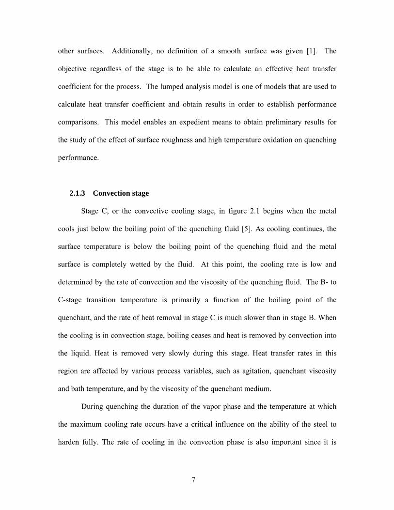
2.1.3 Convection stage
Stage C, or the convective cooling stage, in figure 2.1 begins when the metal
cools just below the boiling point of the quenching fluid [5]. As cooling continues, the
surface temperature is below the boiling point of the quenching fluid and the metal
surface is completely wetted by the fluid. At this point, the cooling rate is low and
determined by the rate of convection and the viscosity of the quenching fluid. The B- to
C-stage transition temperature is primarily a function of the boiling point of the
quenchant, and the rate of heat removal in stage C is much slower than in stage B. When
the cooling is in convection stage, boiling ceases and heat is removed by convection into
the liquid. Heat is removed very slowly during this stage. Heat transfer rates in this
region are affected by various process variables, such as agitation, quenchant viscosity
and bath temperature, and by the viscosity of the quenchant medium.
During quenching the duration of the vapor phase and the temperature at which
the maximum cooling rate occurs have a critical influence on the ability of the steel to
harden fully. The rate of cooling in the convection phase is also important since it is

8
generally within this temperature range that martensitic transformation occurs and it can,
therefore, influence residual stress, distortion and cracking.
2.2 Quenchant Chemistry
Oils used for quenching applications include various petroleum distillates
(mineral oil) and animal fats (vegetable oil)-generally mixtures of chemical structures
with a range of molecular weights and thus vary widely in composition, properties, and
heat-removal characteristics, depending on the source and extent of refinement [5]. These
oils may also be blended with various additives. Some data show that quenching oils,
whether mineral or fat derived, can be formulated to produce similar quenching
properties [5]. The quenching with vegetable oils is beneficial to the environment, but
availability, price, stability and quenching performance currently favor the selection of
mineral oils [5].
2.2.1 Mineral oils
Mineral oils have been used as quenchant for a long time since a wide range of
quenching characteristics can be obtained through careful formulation and blending of
the oils and additives. Mineral oils can be any petroleum oil, as contrasted to animal or
vegetable oils. Also a highly refined petroleum distillate, or white oil, used medicinally as
a laxative. Mineral oils used in quenching are analogous to other petroleum products,
including engine oils, spindle oils, and industrial lubricating oils such as gear lubricants.
[6] Although petroleum oils are usually refined for specific applications, they remain
complex mixture with a variety of possible compositions, which may vary even when
produced by a single refinery [5].

9
The complexity of a quench oil can be shown by gas chromatography, an
analytical technique that separates mixtures based on differences in component volatility
and adsorptivity. The complexity of the mixture, or the number of individual
components, can be determined by counting the number of peaks in the chromatogram,
which provides a characteristic “fingerprint” of the oil [5]. The chromatographic
complexities of the Wolfson reference quench oil that has been proposed as a standard for
the International Organization for Standardization draft on quench oil [7]are illustrated in
figure 2.3 [8].
Fig 2.3 Gas chromatogram of the wolfson reference quench oil [5]
The components of a petroleum oil are many, including paraffinic, naphthenic,
and various oxygen-, nitrogen-, and sulfur-derived open-chain and cyclic derivatives. The
specific composition of a petroleum oil varies with the source of the crude oil. Generally
the mineral oils are distilled from the C26 to C38 fraction of petroleum and composed of
branched paraffins (CnH2n+2) and cycloparaffins (CnH2n) together with a small amount of

10
aromatics (Benzene ring and its derivatives). Within individual molecule, there are some
cycloparaffin rings, aromatic rings and the necessary paraffin and olefin side or
connecting groups. The difference in the cooling performance from oil to oil has much to
do with how much unsaturated components with the oil.
Fig 2.4 Expected hydrocarbons in a typical crude oil fraction [5]

11
The volatility of components in an oil, which is usually inversely proportional to
its flash point, decreases as the average molecular size or carbon number of the
components increases [5]. Figure 2.4 lists several petroleum oil components and their
relative volatilities. The more volatile a component, the lower its flash point.
Fig 2. 5 Cooling rate curves of various quench oils at 60oC [5]
The compositional complexity of quench oils affects their quenching
performance. Segerberg [9] compared a series of mineral-oil-base quenchants under
standard conditions and obtained a wide variety of cooling rates as shown in figure 2.5. It
is clear that even straight mineral oils vary in quenching performance. Formulated oils
can produce an even wider range of cooling rates.
Windergassen [10] reported that quenching oils that contain substantial quantities
of naphthenic derivatives usually exhibit inferior cooling characteristics, a greater
deposit-forming tendency, and lower flash points than paraffinic oils. The lower flash

12
points are particularly deleterious in heat-treating applications. Protsidim et al [11]also
showed that small changes in the compositions of the quench oils resulted in significant
changes in quenching properties. Tensi [12] has shown that the quench severity of a
particular oil is directly related to its ability to wet a metal surface. Usually the particular
additive or combined additive is added into the oil to accentuate the wettability of an oil,
thus having a dramatic effect on oil properties including sludging, staining and so forth.
The wettability of an oil can be quantified by measuring “rewetting” time or measuring
the contact angle of the oil on that surface.
2.2.2 Vegetable oils
Although mineral oils have traditionally been one of the most commonly used
quenching media, unlike water, they are being subjected to ever-increasing controls due
to increasingly stringent governmental regulations regarding their use [13]. Routine
disposal and inadvertent release into the environment, especially into the soil where they
may leach into drinking water aquifers, is being increasingly regulated by governmental
agencies. Thus far, the most commonly cited basestocks for the formulation of
environmentally friendly quenchants are vegetable oils including canola oil and soybean
oil derivatives and so on [14].
Vegetable oils are compounds of carbon, hydrogen, and oxygen, which are found
naturally in all plants. Vegetable Oils are defined as liquid glycerides, which is also
called ‘salts of organic acids’ and generally consist of three kinds of substances:
Saturated fat, polyunsaturated fat, and Monounsaturated fat.

13
Vegetable oils are typical natural occurring triglycerides with the generic structure
shown in figure 2.6. Each vegetable oil is characterized by the particular type and
concentration [13]. Oil is removed from the vegetable beans (or seed) in an “expelling”
process [13]. Expelling can be performed by either pressing the bean (or seed) or, more
commonly, by a solvent extraction process. Expulsion by solvent extraction is a three-
step process: bean preparation, oil extraction and solvent stripping, and reclamation.
Fig 2.6 Vegetable oil triglyceride structure [13]
The triglyceride structure of vegetable oils in figure 2.6 can be generated by the
following chemical reaction of the radicals of (CH3) 3-(CH2) 3n-C3H5 with such organic
acids as CnH2n-1COOH, e.g. Oleic acid (C17H33COOH))[15]. “n” is the integer equal to
or greater than 1.
− CH2 + Organic acid CnH2n-1COOH = Triglycerides CnH2n-1COOCH2
− CH CnH2n-1COOCH
− CH2 CnH2n-1COOCH2
The different kinds of oils found in nature are due to the number of fatty acids.
One kind of oil generally has some kind of predominant acid in it, and along with this
predominant acid it will have besides a number of the other acids in smaller amounts

14
[15]. The different acids each have different properties, and impart these differences to
the oils in which they occur.
No oil has any fixed combination of the different fatty acids present in it, but the
proportions of these will vary with locality, soil, season, and other factors. This accounts
for differences between the same species of oil from different places, or harvested at
different times [15].
The following is the list of common fatty acids and their source [15].
• Lauric acid- cocoanut, palm nut
• Oleic acid-most vegetables: C17H33COOH
• Linolenic acid- linseed and drying oils: C17H31COOH
• Stearic acid: C17H35COOH
• Palmitic acid- palm and vege and animal. : C15H31COOH
• Arachidic acid- peanut.
‘Drying’ is defined as readiness with which they absorb oxygen.
• Drying oils: Linseed prilla, Tung, Chinese wood, Soya.
• Semi-drying: Cottonseed, Corn, Sesame, Rape.
• Non-drying: Peanut, Olive, Castor, and Almonds.
Iodine number is defined as the number of milligrams of iodine absorbed by 1
gram of oil. The iodine value and the absorbing power of oxygen run parallel. Iodine
number can be used to identify the oil [15].
2.3 Quenchant Characterization
Quenching is a critical step in the production of heat treatable steel alloys. In most
cases the most rapid quench from the solution heat treatment temperature is required to

15
develop the best properties, but quite often lower quench rates are used to minimize
residual stress from the quenching operation. In 1968 Vruggink reviewed methods of
evaluating the effects of quench rate on mechanical properties, and concluded that the
simplest and most effective method was to quench in different media.
Fig 2.7 Transformation diagram of low- alloy steel with cooling curves for various quenching media [5]
Figure 2.7 shows a sample transformation diagram of low alloy steel with cooling
curves for various quenching media.
In figure 2.7, curve A shows water or brine used as a quenchant. It is fast enough
to avoid the nose and full transformation to Martensite is attained. The fast oil shown in
curve B, although slower than the water, also attains full Martensite transformation. Both
A and B reach the Martensite start and Martensite finish temperature without touching
the nose. Conventional oil, hot water, and air do not accomplish this and thus do not
form a pure Martensitic structure. The product will have a mixture of phases.

16
The three cooling stages were observed by Scott in his studies. The studies
showed three distinctive mechanisms of heat dissipation. In general the fundamental
properties of liquids determining quenching power are thermal conductivity, viscosity,
specific heat, and heat of vaporization [1].
French found that cooling at the surface of steel bodies in liquids at low velocities
is seldom uniform. The effects described suggest the need for cooling rates above the
critical cooling rates for steel to be hardened. This can be accomplished by changing
coolant composition, and to providing adequate circulation and volume of coolant [1].
French was also one of the first to record information on properties of quenchants
in order to properly characterize them. Up to that time, there had been less concern for
gathering of data of the quenching fluids. French provides a list of properties as specific
heat, flash point, fire point, initial boiling point, final boiling point, final vapor
temperature and parts per million of solids. These properties had not been readily
available in the literature at that time.
Prof. Tamura identified four stages of cooling and correlated these four cooling
stages with the specific physical properties of quenchant. [16-19]. The first stage was
difficult to observe due to the initial heating up of the small probe. Time in this stage
depends on specific heat, viscosity, thermal conductivity, and difference in temperature
between solution temperature and the boiling point of the liquid. No specific name was
given to this stage except that it is the first one.
The second stage (this is the first stage that is detected most of the time) is the
vapor blanket stage. There is a temperature in excess of the critical overheat temperature
(COHT) this stage ends at the Leidenfrost Point (Characteristic Temperature). This
17
temperature is dependent on the vapor pressure, latent heat, boiling point, viscosity, and
activity of the liquid towards the probe surface.
Third Stage (Nucleate Boiling) has the highest cooling rate. Cooling in this stage
depends on the boiling point of the liquid.
Fourth Stage (Convection Cooling), which exhibits the lowest cooling rate, is
affected by the difference of the viscosity and temperature difference of the boiling point
and the temperature of the liquid. Cooling rate increases if: critical temperature, latent
heat, and wettability increase, and if vapor pressure and viscosity are decreased.
He also conducted a simultaneous investigation of the cooling process and
generation of surface and center cooling curves by movie recording of the interfacial
cooling process at the quenched hot metal surface. These results were correlated with
chemical and physical properties of the liquid quenching media.
Tamura created the concept of Master Cooling Curves. The cooling curves
obtained from a probe depend on the cooling characteristics of the quenchant, thermal
constants, and size and shape of the probe. Tamura developed the Master Cooling Curve
concept that is only dependent on the quenching oil. This methodology was developed
from the results of experiments done with steel and silver probes. The methodology
permits the evaluation of the oil performance without the effects of the size and the
material of the probe. Prof. Tamura found that the Characteristic Temperature
(Leidenfrost) and the convection start temperature of surface cooling curves are
independent of probe size, and the cooling speed changes as a function of the size of the
probe. Center cooling curves have a more complicated behavior not [20].

18
The use of the cooling curve analysis improved the quenchants and heat treatment
technologies in Japan Prof. Tamura studied the cooling ability of various aqueous liquids,
animal and vegetable oils, as well as mineral oils. He compared mineral and fatty oils,
studied deterioration of quenching oils, thermal decomposition and polymerization, and
use of oxidation inhibitors [20].
Tamura also studied ability of aqueous solutions in oils, aqueous solutions, and
animal and vegetable solutions [21]. Tamura found that rich solutions of non-volatile
solutes of MnSo4 and Na2CO3 increase the cooling rate considerably, in the 700-500 °C
range and reduce it at 300°C relative to distilled water.
He determined the cooling ability of animal and vegetable oils. Increasing
molecular weights decreases vapor pressure, increases boiling point and critical
temperature, and reduce the vapor blanket stage. In general, increasing molecular weight
reduces the ability to differentiate the four stages of cooling. An increase in the aromatic
hydrocarbon in mineral oils of similar molecular weight decreases vapor pressure,
increases the critical start temperature and boiling point, as well as the wettability.
Naphthenic cooling rates are greater than parafinic [22].
Prof. Tamura studied extensively the effects of distillation, hydrocarbon types,
and refining on the cooling curve behavior of mineral oils. The addition of lighter oil
will reduce the characteristic temperature (Leidenfrost Temperature). The cooling curves
of unrefined oils exhibit slightly higher critical temperatures and higher cooling rate,
probably caused by adsorption of impurities and the difference of viscosity at a higher
temperature range [22].

19
Tamura also studied the deterioration of quenching oils. Oil deterioration is
accompanied by a change in cooling rates, surface discoloration, formation of sludge, and
decrease in flash point. He performed a detailed investigation of the degradation
processes of the oil by modeling the oil oxidation and thermal decomposition.
Mr. Segerberg has devised a method to rate oils in terms of relative hardening
power with the assistance of a portable quenchant tester [23]. The goal of his work is to
select the quenchant best suited for a particular application. The later section describes
the Relative Hardening Power (HP) by IVF. A formula has been developed using three
characteristic points in the cooling rate curve. These points are: the transition
temperature from film boiling to nucleate boiling, the cooling rate between 500oC and
600oC, and the transition temperature from nucleate boiling to convection. The
quenching system generates the cooling and cooling rate curves and provides the
necessary data to use the IVF hardening power equation. The IVF quenching system that
complies with ISO 9950 is now widely used in industry [23].
2.4 Quenching probes
The quenching probes have been produced in a great variety of shapes, including
cylinders, spheres, square bars, plates, rings and coils, round disks and production parts.
Also the probes have been constructed of various materials, including alloy and stainless
steels, silver, nickel, copper, gold and aluminum [5].
2.4.1 General Motors (GM) quenchometer
The cooling rates produced by quench oils are often classified on the basis of the
GM quenchometer or nickel ball test [24, 25]. The GM quenchometer, which can

20
measure the heat removal properties of the quenchants, uses the Curie temperature of a
metal as a means to obtain a characterization of a quenching fluid. The Curie temperature
is the temperature at which a metal becomes magnetic.
Fig 2. 8 GM quenchometer and principle of operation [5]
Details of this test are given in ASTM Standard D 3520. The test involves heating
a 22mm diameter nickel ball to 885oC and then dropping it into a wire basket suspended
in a beaker containing a 200mL of the quenchant oil at 21 to 27oC [26]. A timer is
activated as the glowing nickel ball passes a photoelectric sensor [5]. A horseshoe magnet
is located outside the beaker as close as possible to the nickel ball. As the ball cools, it
passes through its Curie point (354oC), the temperature at which it becomes magnetic [5].
When the ball becomes magnetic, it is attracted to the magnet, activating a sensor that
stops the timer, as shown in figure 2.8.

21
The cooling time needed to reach Curie temperature is referred to as heat
extraction rate or quenchometer time. The oils are then classified in slow, medium and
fast [5]. The classification is slow oils 15-20 seconds, medium oils 11-14 seconds and
fast oils 8-10 seconds [1].
2.4.2 Grossmann Probe
One of the earliest probes used is shown in figure 2.9 [27]. This probe was
constructed from a 100x300mm (4x12in) SAE 5145 alloy by cutting it in half, yielding
two 100x150mm sections. A chromel-alumel thermocouple was hydrogen brazed to the
center of the bottom half. The thermocouple wires were passed through a 13mm hole
drilled through the top half of the bar. A steel tube, used as a handle, was welded to the
top section, and both sections were then welded together. The cooling time-temperature
data were collected using Speedomax equipment manufactured by Leeds & Northrup
Company.
Fig 2.9 SAE 5145 Steel Probe used by Grossmann [27]
2.4.3 IVF probe
The IVF probe is based on the ISO9950 standard and is manufactured by the
Swedish Institute of Production Engineering Research. The probe and system are
described in the following paragraphs. The information in table 2.1 has been summarized
from IVF Quench test, portable test equipment for quenching media [28].

22
Figure 2.10 shows IVF probe. The test probe is fastened to the handle using a
standard thermocouple plug-and-socket connection. This allows measurement to be
made, for example, with thermocouples embedded in components.
Table 2. 1 IVF Probe Characteristics [28]
IVF PROBE
Probe size Probe body: Φ12.5 mm x 60 mm
Overall Length: 600 mm Material Inconel 600 Thermocouple Location Center along long axis
Weight Handle 0.45kg, test probe 0.35kg Acc./Fixtures Handle with start button ISO 9950 Compliant Yes
Fig 2.10 IVF test probe and handle [28]
IVF probe has many applications due to its portability; these applications can be
listed as follows [28]:
On-site measurement of the cooling characteristics of a quenchant, directly in the
quench tank, so as to test the cooling performance at various positions in the

23
quench tank, check the effect of the rate of flow on cooling performance and
follow changes in the cooling performance of a quenchant.
Laboratory measurements
Tests with different quenchants e.g. oils, polymers, water and salt
Incoming inspection of quenchants
2.4.4 The Drayton Probe
The following tables and paragraphs describe the Drayton Probe System. The
system is used for routine quality testing, diagnostic work, safety checks, process control,
quenchant selection and development of new formulations. The data has been
summarized from Drayton Probe Systems: Quenchalyzer [29]
Table 2. 2 Drayton Probe Characteristics [29]
Drayton Probe
Probe Size 12.5 mm Diameter x 60 mm length
Overall Length 375 mm, 750 mm
Material Inconel 600
T/C Location Center along long axis
Acc./Fixtures None
ISO 9950 Compliant Yes Drayton probe and the portable quenching system can be seen in figure 2.11. This
system has the key features and benefits: in-plant or laboratory use; static or agitated
testing; suitable for oils, aqueous polymers, salt or brine; high level of test reproducibility
and consistency; extensive windows based software; provides instant graphic and
numeric comparisons.

24
Fig 2.11 Drayton probe and the portable quenching system [29]
2.4.5 Nanigian-Liscic Probe
The LISCIC -NANMAC probe, as shown in figure 2.12, is a cylindrical probe
200 mm long and 50 mm in diameter. It is made of AISI304 steel and is instrumented
with three thermocouples placed on the same cross-section plane in the middle of the
probe’s length. One thermocouple is placed at the surface. This thermocouple is a
special type, which utilizes flat ribbon and is known as “self-renewing” thermocouple.
The second thermocouple is placed at 1.5 mm below the surface and the third one at the
center of the cross-section. This probe is reported to be particularly sensitive for
measuring heat flux during quenching because it measures the temperature gradient from
the surface to the center of the probe. The key feature of this probe is that it measures
and records the temperature on the very surface of the probe, with a very response time of
(10-5 sec.). The probe is capable of recording fast changing temperatures.
The software used with the probe (TGQAS) calculates heat transfer coefficients
on the probe surface and cooling curves in any arbitrary point of the round bar cross-
25
section of different diameters. The software also predicts microstructure and hardness in
any of those points after quenching, for every steel grade the CCT diagram of which are
stored in the software.
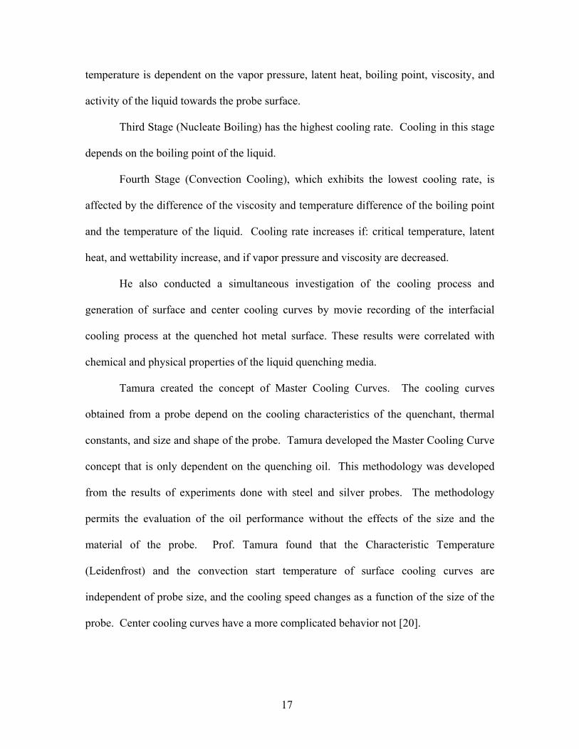
Fig 2.12 Schematic of Liscic-NANMAC probe--TGQAS Temperature Gradient Quenching Analysis System by Prof. Bozidar Liscic [1]
2.4.6 Tamura’s Probes
In order to gain insight into the quenching process, it has been proposed that it is
critically important to model the heat-transfer properties that occur at the metal surface
during quenching. In such an analysis, the quenchant is considered to be a heat-transfer
fluid that controls the rate of heat loss over the range of metal temperatures during the
quenching cycle. Thus, the heat-transfer properties of the quenchant determine the
metallurgical properties obtained [5].
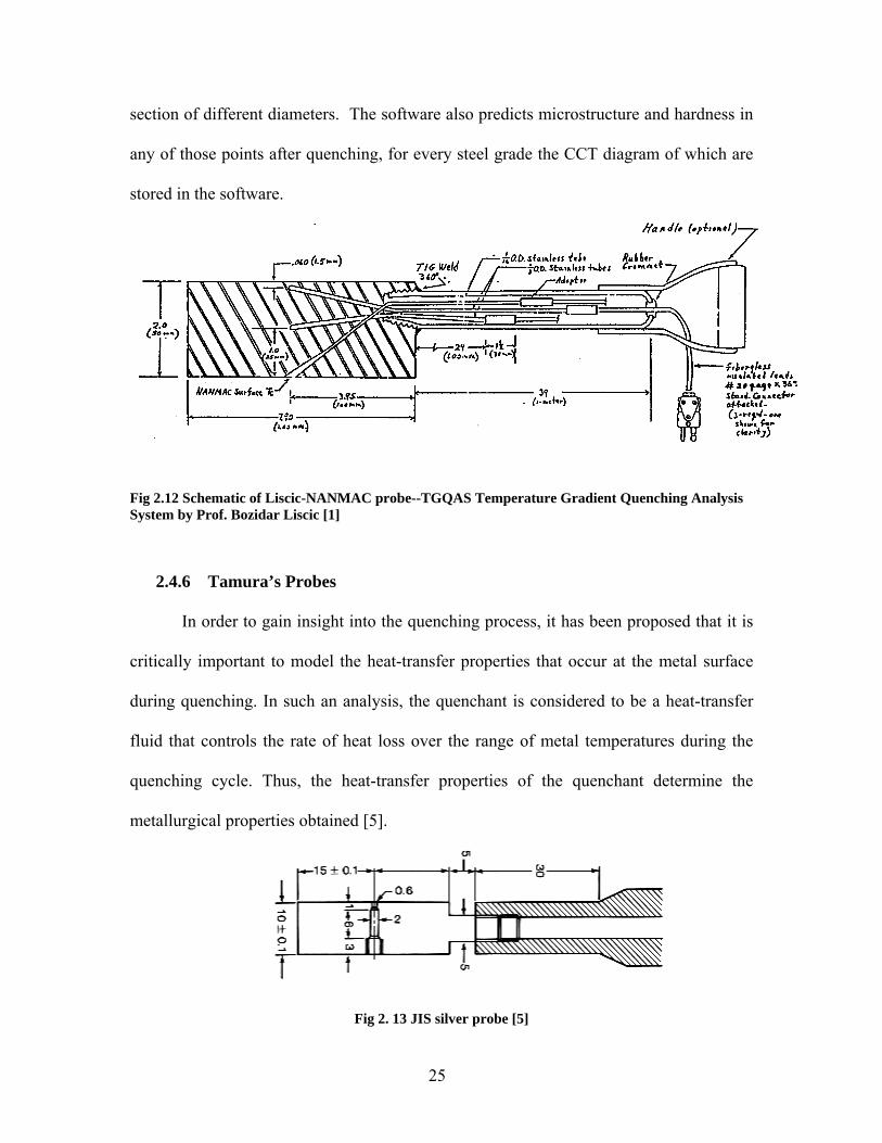
Fig 2. 13 JIS silver probe [5]

26
Tagaya and Tamura [30] developed a Japanese Industrial Standard (JIS) for
cooling curve acquisition that utilizes a cylindrical silver probe with a thermocouple
assembly specifically constructed to determine the surface temperature change with time
during quenching. The JIS probe, as shown in figure 2.13, was used by Tamura in his
classic work describing the development of master cooling curves [30] and quench oil
characterization [31], but it has not gained wide acceptance in Western industry since the
concern has been expressed regarding the cost of silver used in the probe construction,
problems in maintaining a clean surface and the comparative difficulty of preparing
delicate surface thermocouple assemblies.
2.5 Cooling curve analysis
Various methods have been developed to simplify the measurement of cooling
power, including the General Motors (GM) quenchometer, the hot wire test, the 5-second
interval test, and the cooling curve test. Of these procedures, the cooling curve test has
been generally accepted as the most useful means of describing the mechanisms of
quenching [32]. Cooling curves are particularly sensitive to factors that affect the ability
of quenchants to extract the heat, including quenchant type and physical properties, bath
temperature and bath agitation.
2.5.1 Data Acquisition and Cooling Curve Analysis
The need to acquire sufficient data to adequately define a cooling curve for
subsequent analysis has long been recognized. Special data acquisition devices, including
hardware such as oscillographs, were used for work reported by Jominy, French and

27
others [5]. However, this equipment is difficult to calibrate, which has inhibited
widespread use of cooling curve analysis. Currently, sufficient data acquisition rates can
be achieved with personal computers equipped with analog-to-digital (A/D) converter
boards.
Although computer hardware is available, there are no published guidelines for
selecting a data acquisition rate, which varies with probe alloy, size and quench severity.
Probably the best method for selecting the required acquisition rate is to determine it
experimentally [5]. This can be done by repeatedly quenching a probe in cold water, one
of the more severe quenchants, and collecting data at various acquisition rates and
comparing which data acquisition rate can give a smooth cooling rate curve in the
maximum cooling rate region. Although higher data acquisition rates are preferred, they
may lead to data storage problems.
After sufficient data are collected, cooling curve analysis can be started. Cooling
curves are relatively easy to obtain experimentally by using an apparatus that typically
consists of an instrumented probe and a system for data acquisition and display. Such
system can be purchased or custom built. Either way, it is important that the user
understand the basic system components [5]. One of the most important components is
the quench probe used for cooling curve acquisition. There are a variety of quenching
probes, as mentioned in section 2.4. To choose which kind of probe to use depends on the
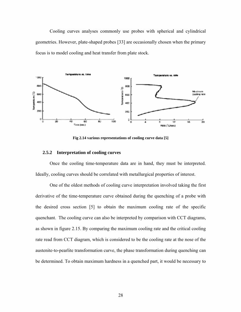
specific condition and requirement. Figure 2.14 shows two representations of the cooling
curve data. The cooling data can be plotted as time-temperature, cooling rate-temperature
or cooling rate-time curves.
28
Cooling curves analyses commonly use probes with spherical and cylindrical
geometries. However, plate-shaped probes [33] are occasionally chosen when the primary
focus is to model cooling and heat transfer from plate stock.
Fig 2.14 various representations of cooling curve data [5]
2.5.2 Interpretation of cooling curves
Once the cooling time-temperature data are in hand, they must be interpreted.
Ideally, cooling curves should be correlated with metallurgical properties of interest.
One of the oldest methods of cooling curve interpretation involved taking the first
derivative of the time-temperature curve obtained during the quenching of a probe with
the desired cross section [5] to obtain the maximum cooling rate of the specific
quenchant. The cooling curve can also be interpreted by comparison with CCT diagrams,
as shown in figure 2.15. By comparing the maximum cooling rate and the critical cooling
rate read from CCT diagram, which is considered to be the cooling rate at the nose of the
austenite-to-pearlite transformation curve, the phase transformation during quenching can
be determined. To obtain maximum hardness in a quenched part, it would be necessary to

29
select a quenchant that produces a maximum cooling rate equal to or greater than the
critical cooling rate.
Fig 2.15 CCT diagram for a spring steel (50M7) with superimposed cooling curves [5]
Liscic [34] demonstrated that one method of obtaining a useful correlation
between cooling rates during a quench and hardness was to integrate the area under
cooling rate curves. A plot of accumulated area versus time can then be used to quantify
the progression of the quench cycle. Thelning [35] reported a similar method involving
the integration of the area under the cooling rate curve between two temperatures, e.g.
600 to 300oC.
To simplify cooling curve interpretation, Tamura et al. developed a quantity
called the “V-value”, which is proportional to the ability of an oil quenchant to harden
steel [31]. The cooling rate can also be related to Grossmann quench severity factor,
which is an indication of the hardness of the as-quenched specimen, and such quenchant
performance indices as hardening power, Castrol index and quench factor, which will be
discussed in detail in section 2.7.

30
2.6 Metallurgy of 4140 Steel and 304 Stainless Steel
2.6.1 Characteristics and TTT diagram of 4140 steel
According to their carbon content, the plain carbon steel can be categorized as
high-carbon steel (>0.60%), medium-carbon steel (0.30-0.60) and low-carbon steels
(<0.30%). [36] 4140 can be classified as the medium-carbon steels with the chemical
composition of 0.38-0.43 C by weight.
AISI 4140 steel is made with chromium and molybdenum alloy additives.
Chromium from 0.5 to 0.95% is added with a small amount of molybdenum (from 0.13 to
0.20%). These small amounts of these two elements increase the strength, hardenability
and wear resistance of the 41xx series of alloy steels [37].
The chemical composition and typical applications of 4140 steels are listed
below: AISI-SAE 4140 steel has 0.40 % Carbon, 0.58% Manganese, 0.95% Chromium,
and 0.20% Molybdenum. Low alloy steels with chromium and molybdenum, because of
their increased hardenability, can be oil quenched to form martensite instead of being
water quenched since the slower oil quench reduces temperature gradients and internal
stresses due to volume contraction and expansion during quenching. Distortion and
cracking tendencies can be minimized.
4140 is among the most widely used medium-carbon alloy steels. Relatively
inexpensive considering the relatively high hardenability 4140 offers. Fully hardened
4140 ranges from about 54 to 59 HRC, depending upon the exact carbon content.
Forgeability is very good, but machinability is only fair and weldability is poor, because
of susceptibility to weld cracking [38].

31
Time, sec
100 101 102 103 104 105 106
Tem
pera
ture
, o F
200
400
600
800
1000
1200
1400
1600
Fig 2. 16 TTT diagrams of AISI 4140
Figure 2.16 is TTT diagram of AISI 4140, which indicates the phase
transformation from austenite to martensite or bainite or pearlite depending on the
cooling rate that can be achieved from specific quenchant. Such diagram is valuable since
the cooling curve can theoretically be superimposed upon it to predict heat-treatment
response. The steel begins to transform at the Ms Temperature and is fully hardened at
the Mf temperature.
The starting and ending temperature of martensitic transformation Ms and Mf,
which is quite critical for understanding of quenching process of 4140 steels, can be read
from the diagram. Ms = 640oF = 337.78oC and Mf = 425oF = 218.33 oC. Also in order to
get the complete martensite and avoid the formation of pearlite or bainite, the quenchant

32
must be able to cool the component fast enough to miss the nose of the curve for pearlite
formation.
The microstructure of alloy 4140 after being fully annealed at 691°C consists of a
blocky ferrite and course pearlite. After austenitizing at 843°C and oil quenching a
martensitic structure is produced and with subsequent tempering at 315°C, a fine
tempered martensitic structure is the result. Martensite in low alloy steels consists of
packets of fine units of martensite called laths that align themselves parallel to one
another to form packets [37]. The orientation of the units or laths within a packet is
limited, and frequently large volumes of laths within a packet have only one orientation.
Therefore many of the boundaries within a packet are low-angle and as an approximation,
the entire packet has essentially one orientation.
The mechanical properties of normalized and annealed low-alloy AISI 4140 steel
are the following [1]:
Table 2. 3 Mechanical properties of normalized and annealed 4140 [1]
AISI No
Treatment
Yield
Strength (psi)
Tensile Strength
(psi)
Elongation
%
Reduction in area %
Hardness
.Bhn
Impact Strength (IZOD)
ft-lb Normalized (1600 °F) 95000 148000 17.7 46.8 302 16.7
4140 Annealed (1500 ° F) 60500 95000 25.7 56.9 197 40.2
Table 2. 4 Mechanical Properties of quenched and tempered 4140 steels [1]
AISI No
Tempering Temp. °F
Tensile strength
(psi)
Yield Strength
(psi)
Elongation
%
Reduction in area %
Hardness
Bhn 400 257000 238880 8 38 510 600 225000 208000 9 43 445 800 181000 165000 13 49 370 1000 138000 121000 18 58 285
4140
1200 110000 95000 22 63 230

33
2.6.2 Characteristics of 304 stainless steel
The stainless steels can be categorized by a structure nomenclature: Austenitic,
Ferritic and Martensitic stainless steels [39]. The austenitic stainless steels represent the
largest group of stainless steels in use, making up 65 to 70% of the total for the past
several years. The austenitic alloys used most often are those of the AISI 300 series.
Collectively, these enjoy their dominant position because of a general high level of
fabricability and corrosion resistance and because of the varied specific combinations of
properties that can be obtained by different compositions within the group, providing
useful material choices for a vast number of applications. Types 302 and 304 have
somewhat greater stability and improved corrosion resistance [39]. Type 304, one of the
alloys of AISI 300 series based on the Fe-Cr-Ni ternary system, is the most widely
produced stainless steel and is used considerably at elevated temperatures.
According to the ternary diagram for Fe-Cr-Ni system, generally compositions
approximating the leaner AISI 300-series stainless steels would be predicted to fall either
within the α+γ field or just outside of it, depending on the specific composition. Figure
2.17 is the cross sections of Fe-Cr-Ni ternary, which reveals how the shape of the
austenite (γ) field changes with increasing total nickel plus chromium contents. At 70,80
and 90% iron, the γ/(α+γ) boundary slants backward such that a fully austenitic alloy
close to boundary at 1000oC can contain some ferrite when heated. For type 304,
according to its composition 18-20% Cr, 8-12%Ni, it is within α+γ region below 1300oC,
as shown by the arrow in the figure, which means if 304 type of probe is quenched at
850oC, then quenching process will start with α+γ.

34
Fig 2. 17 Cross sections of Fe-Cr-Ni ternary diagram [39]
2.6.3 Theoretical understanding of heat transfer
Heat transfer during quenching of hot metal parts is controlled by different
cooling mechanisms at three different quenching stages: film boiling, nucleate boiling
and convection, as mentioned in the previous sections. The parameters that affect the
heat transfer during quenching in liquid quenchant will be identified and discussed below
phase by phase.
2.6.3.1 Film boiling heat transfer
Upon immersion into the quench fluid, the part will first be surrounded by vapor
blanket; the quenching starts with the film boiling. In this range heat transfer rate is
minimum and heat transfer occurs mainly through radiation. The part cools slowly in this
304

35
regime. As the part cools, film becomes unstable and the mechanism is then called partial
film boiling or transition boiling.
The total heat transfer coefficient during film boiling is generally expressed as the
sum of a convective coefficient, hc, and an effective radiation coefficient (fhr), where f is
a constant. The heat transfer coefficient has different expressions depending on the
geometry and orientation of the part being quenched. For Film boiling on horizontal
plates, Sciance et al [45] model is found to be very good when compared with
experimental results on four organic liquids. For minimum heat flux in the film boiling
regime, the equation for convective heat transfer coefficient using this model is
( ) ( )( ) ( )[ ]
−
−′= 2/1
3
425.0GLcsatwG
GLGfgGc ggTT
gHkh
ρρσµ
ρρρ
This equation can also be expressed in generalized form as
( ) ( ) ( )
4/14/1*425.0
fsatwpG
fgfBfB TTc
HRaNu
−
′= Eqn. 2.6.3-1
Where ( )G
cB k
BhNu =
( )
( )
−=
=
G
GpG
G
GLG
GBB
kcgB
GrRaµ
µρρρ
2
3
** Pr
B = Laplace reference length = ( )
2/1
− GL
c
gg
ρρσ
And f (subscript) means that the physical properties of the vapor are evaluated at pressure
pL and temperature Tf.
For Film Boiling on horizontal cylinders, Sciance et al [45] suggested the
following correlation for horizontal cylinder

36
( )( ) ( )
267.0267.0
2
*
369.0fsatwpG
fg
fr
BfB TTc
HTRaNu
−
′
= Eqn. 2.6.3-2
Which is based on their study of methane, ethane, propane and n-butane on the surface of
horizontal gold-plated cylinder 0.81 in. in diameter by 4 in. long.
For Film Boiling on a Vertical Surface, Bromley [46] recommended an equation
very similar to Eqn. (2.6.3-2), with a change in the characteristic length D and L is the
vertical distance from the bottom of the plate. Hsu and Westwater [47] modified the
correlation considering boundary layer above the heated surface and its transition from
laminar to turbulent flow. The correlation becomes
( ) ( ) ( )[ ]( )
2/122/1* 34.01
943.0
−
−+=
satwpG
fgsatwpGfgfLfL TTc
HTTcHRaNu Eqn. 2.6.3-3
Equations 2.6.3-1, -2 and-3 can be combined together and simply represented with the
following form:
( ) ( ) ( )
n
satwpG
fgmLB TTc
HARaMNu
−
′= Eqn. 2.6.3-4
Where M, A, l and n are constants. From equation 2.6.3-4 and the definition of Ra
number, it can be seen that heat transfer coefficient can be affected by such factors as the
viscosity of vapor film and the liquid quenchant, surface tension, the density of vapor
film and the liquid quenchant, the latent heat and the specific heat. If these properties are
known, then the heat transfer coefficient in film boiling stage can be calculated. Among
these the heat transfer coefficient is proportional to the reciprocal of the viscosity, which
means the heat transfer coefficient will decrease with the increase in the viscosity of the
quenchant, given other properties constant.

37
2.6.3.2 Nucleate boiling heat transfer
With further decrease in temperature, partial films are broken into numerous
bubbles and the quench media contacts the part directly. The liquid near the hot surface
becomes superheated and tends to evaporate, forming bubbles wherever there are
nucleation sites such as tiny pit or scratches on the surface. The bubbles transport the
latent heat of the phase changes and also increase the convective heat transfer by
agitating the liquid near the surface. This corresponds to rapid heat transfer. The part is
still very hot and the quench media boils vigorously. In this regime, heat transfer is very
high for only a small temperature difference.
The heat removed from the heated surface by the boiling liquid is assumed to be
by the following mechanisms:
(i) heat absorbed by the evaporating microlayer ( MEq );
(ii) heat energy expended in re-formation of the thermal boundary layer ( Rq ) and
(iii) heat transferred by turbulent natural convection ( NCq ).
The total boiling heat flux is obtained from the above three fluxes [48] as
NCwg
wRgMEtot q
tttqtq
q ++
+= Eqn. 2.6.3-5
The heat flux associated with the microlayer evaporation [49] is given by
( )
⋅=
ANHtJaArBq fglglME ραπγφ 2/327.02
10 Eqn. 2.6.3-6
Where AN / is the nucleation site density,
=
plll
psss
CkCk
ρρ
γ ,
−=
2
1DDdφ and dD
is the diameter of the dry area under the bubble.

38
( )Gfg
bwLp
HTTc
Jaρ
ρ −= , Ar = ( ) ( ) 2/32 gg ll ρσν ⋅ .
The heat flux associated with the thermal boundary layer re-formation [49] is
( )satww
plllR TTa
AN
tCk
q −⋅
⋅⋅
=
πρ
2 Eqn. 2.6.3-7
Using the heat transfer coefficient McAdams [50] estimated in turbulent natural
convection, the heat flux due to turbulent natural convection can be estimated from
( ) ( )satwl
NC TTaANGr
Lkq −⋅
⋅
−⋅= 1Pr14.0 3/1 Eqn. 2.6.3-8
From the expressions in equations 2.6.3-5,6,7 and 8, it can be said that the kinetic
viscosity, density, specific heat, latent heat, the temperature between the heated part and
the quenchant, surface tension and the thermal conductivity are playing important roles in
the calculation of heat flux (heat transfer coefficient). Also the heat flux is proportional to
(1/ν) n, which indicates the heat flux increases as the kinetic viscosity decreases.
2.6.3.3 Convection heat transfer
The last regime is the natural convection regime; the surface of the part has
cooled to a temperature below the boiling point/range of the quench media. The heat is
transferred by the natural convection of the liquid.
Churchill [51] suggested a general convection correlation that is applicable to a
variety of natural convection flows for which the primary buoyant driving force is
directed tangential to the surface. The correlation is given by
( )26/1Pr)(331.0 LL GrbaNu += Eqn. 2.6.3-9

39
Where, ( )[ ] 27/816/9Pr/5.01
17.1
+=b
( )
−= ∞
2
3
νβ xTTgGr w
x
L
pL k
cPr
ν=
The empirical constant a varies for various geometries [51].
In convection stage, equation 2.6.3-9 shows the heat transfer can be related to the
kinetic viscosity, the specific heat, the thermal conductivity, the coefficient of thermal
expansion, the temperature difference between the hot metal part and the liquid and also
the distance from the leading edge of the boundary layer formed on the heated surface x.
In summary, many physical properties of the quenchant affect the calculation of
heat transfer coefficient during the quenching process: the viscosity, the specific heat, the
surface tension, the density, the latent heat and the thermal conductivity. From these
values the heat transfer coefficients can be calculated for each quenching stage. However,
some of these properties are very hard to measure. Among these physical properties, the
viscosity of the quenchant is relatively easier to obtain and also plays an important role in
the calculation of heat transfer coefficient since it is proportional to the reciprocal of heat
transfer coefficient. Therefore, the quenching performance of the mineral oil based
quenchant is correlated with their viscosities in this work to determine how heat transfer
coefficient changes with the viscosity.
Table 2.5 gives the definition of all the variables shown in the above equations.

40
Table 2. 5 Nomenclatures a area of influence of the bubble on the
heating surface
Tb boiling temperature
A area of the heating surface V velocity
Ar Archimedes number ∆p pressure drop
B constant α thermal diffusivity
Cp specific heat at constant pressure γ a parameter
D instantaneous bubble diameter δ Boundary/thermal layer thickness
Db departure diameter of the bubble µ viscosity
Dd diameter of dry area under the bubble λ latent heat of vaporization
G Volumetric flow rate ν kinematic viscosity
g Acceleration due to gravity ρ density
gc Conversion ratio σ surface tension
Gr Grashof number φ parameter
h heat transfer coefficient Subscripts
Hfg Latent heat of evaporation * refers to critical value, or
nondimensional parameter
Ja Jacob number crit refers to critical value
K,k thermal conductivity l liquid
N Number of active nucleation sites sat saturation
P external pressure tot total
Pr Prandtl number v vapor
q,q’’ heat flux w wall
Ra roughness s solid
tg bubble growth time Superscripts
tw waiting time to grow new bubble f Refers to saturated liquid
T temperature fg Refers to phase change from liquid to
vapor
Tw wall temperature g,G Refer to gas or vapor condition
2.6.4 Calculation of heat transfer coefficient
The calculation of heat transfer coefficient is very critical for understanding the
quenching performance of different quenching media. Generally there are three important
modes of heat transfer: heat conduction, thermal radiation and heat convection. But since

41
the thermal resistance to conduction in the solid is small compared to the external
resistance and also the probe tip in our experiments is very tiny, so we may ignore small
differences of temperature within the probe, assume that the spatial temperature within
the system is uniform and only consider the convective heat transfer between probe tip
and quenching fluid. This approximation is called the lumped thermal capacity model
[52]. This model is valid when the Biot number (Bi) is much less than 0.1 and can be
expressed by the following equations:
-hc A (T-Te)= ρ V Cp (T) dT/dt Eqn. 2.6.4-1
Where:
hc=heat transfer coefficient averaged over the surface area, W/m2-K
A=surface area, m2
T=temperature of the wall, oC
Te=temperature of the oil, oC
ρ =Density, kg/m3
V=volume, m3
Cp=specific heat, J/kg*oC
dT/dt=derivative of the temperature with respect to time.
To use cooling rate data to calculate the average heat transfer coefficient the following
must be considered. This solution must assume constant surface area, density, specific
heat, and volume. The specific heat in a quenching application can vary. The density
can also vary but to a lesser extent.
Rearranging equation 2.6.4-1,

42
)()( epc TTdtdTTC
AVh −= ρ Eqn. 2.6.4-2
For cylindrical probe tip,
2*2
*2 rHrHr
AV
==π
π Eqn. 2.6.4-3
Where,
H- height of cylindrical probe tip
r- radius of probe tip
Also, the biot number can be calculated using the equation 2.6.4-4 as follows.
Biot=h Lc/k. Eqn. 2.6.4-4
Where:
h=mean heat transfer coefficient
Lc=Volume/Surface Area, (approximately =radius/2 for a cylinder)
k=thermal conductivity of the steel
For calculation of the heat transfer coefficient in equation 2.6.4-2, ρ , V/A, and Te are
constant, since they are physical properties of the steel or oil. T and dT/dt are
experimental data. However, the specific heat of the steel varies with the temperature.
Therefore, how to choose the specific heat of the steel is important in determining the
heat transfer coefficient. Also in equation 2.6.4-4, the thermal conductivity of the steel is
also critical to calculate the Biot number. The selection of the specific heat and the
thermal conductivity for 4140 steel and 304 stainless steel will be discussed as follows.

43
2.6.5 Thermoconductivity of 4140 steel and 304 stainless steel
Thermal conduction is the phenomenon by which heat is transported from high to
low-temperature regions of a substance. Thermoconductivity is a measure of the rate at
which a material transmits heat. If a thermal gradient of one degree per unit length is
established over a material of unit cross-sectional area, then the thermal conductivity is
defined as the quantity of heat transmitted per unit time [40]. It is best defined in terms of
Fick’s First Law:
dxdTkq −= Eqn.2.6.5.1
Where,
q - Heat flux or heat flow per unit time per unit area, W/m2.
k – thermal conductivity, W/m*K.
dT/dx – Temperature gradient through the conducting medium, K/m
There are a variety of methods for the measurement of thermal conductivity due
to the difficulty of obtaining a controlled heat flow in a prescribed direction such that the
actual boundary conditions in the experiment agree with those assumed in the theory.
Generally these methods fall into two categories: the steady-state and the nonsteady-state
methods. In the steady-state methods of measurement, there are longitudinal heat flow
method, the Forbes’ bar method, the radial heat flow method, the direct electrical heating
method and the thermal comparator method. In the category of nonsteady-state methods,
there are the periodic and the transient heat flow methods [41].
The thermal conductivity, k, is a function of temperature. For 4140, it can be
obtained from two different sources: I) ASM Metals Handbook (1977) [36]. Adding the
polynomial trendline into the scattered data points generated the following polynomial
44
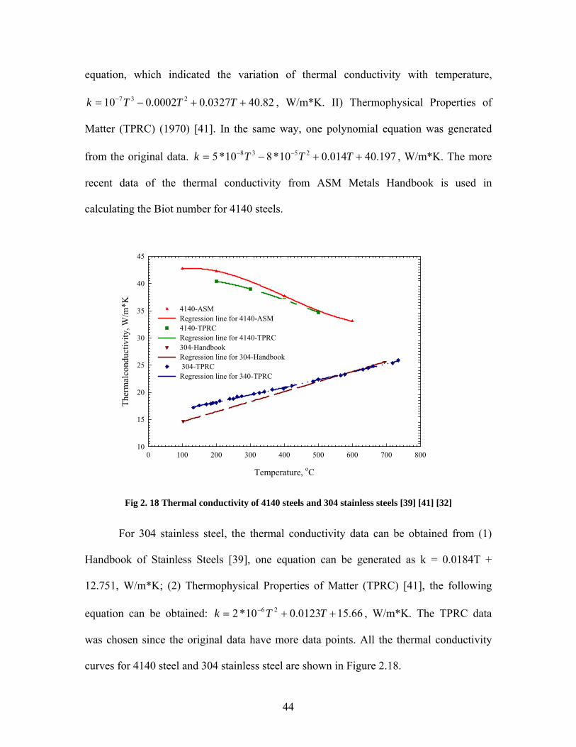
equation, which indicated the variation of thermal conductivity with temperature,
82.400327.00002.010 237 ++−= − TTTk , W/m*K. II) Thermophysical Properties of
Matter (TPRC) (1970) [41]. In the same way, one polynomial equation was generated
from the original data. 197.40014.010*810*5 2538 ++−= −− TTTk , W/m*K. The more
recent data of the thermal conductivity from ASM Metals Handbook is used in
calculating the Biot number for 4140 steels.
Temperature, oC
0 100 200 300 400 500 600 700 800
Ther
mal
cond
uctiv
ity, W
/m*K
10
15
20
25
30
35
40
45
4140-ASMRegression line for 4140-ASM4140-TPRC Regression line for 4140-TPRC304-Handbook Regression line for 304-Handbook 304-TPRCRegression line for 340-TPRC
Fig 2. 18 Thermal conductivity of 4140 steels and 304 stainless steels [39] [41] [32]
For 304 stainless steel, the thermal conductivity data can be obtained from (1)
Handbook of Stainless Steels [39], one equation can be generated as k = 0.0184T +
12.751, W/m*K; (2) Thermophysical Properties of Matter (TPRC) [41], the following
equation can be obtained: 66.150123.010*2 26 ++= − TTk , W/m*K. The TPRC data
was chosen since the original data have more data points. All the thermal conductivity
curves for 4140 steel and 304 stainless steel are shown in Figure 2.18.
45
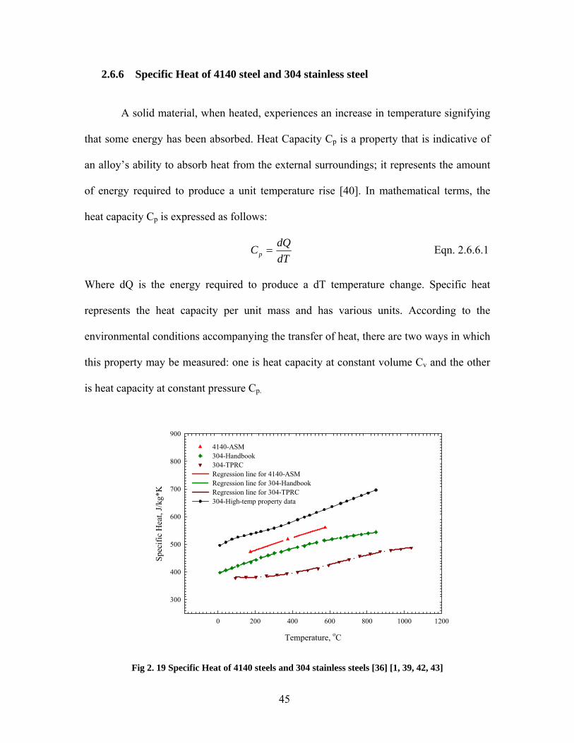
2.6.6 Specific Heat of 4140 steel and 304 stainless steel
A solid material, when heated, experiences an increase in temperature signifying
that some energy has been absorbed. Heat Capacity Cp is a property that is indicative of
an alloy’s ability to absorb heat from the external surroundings; it represents the amount
of energy required to produce a unit temperature rise [40]. In mathematical terms, the
heat capacity Cp is expressed as follows:
dTdQCp = Eqn. 2.6.6.1
Where dQ is the energy required to produce a dT temperature change. Specific heat
represents the heat capacity per unit mass and has various units. According to the
environmental conditions accompanying the transfer of heat, there are two ways in which
this property may be measured: one is heat capacity at constant volume Cv and the other
is heat capacity at constant pressure Cp.
Temperature, oC
0 200 400 600 800 1000 1200
Spec
ific
Hea
t, J/
kg*K
300
400
500
600
700
800
900
4140-ASM304-Handbook304-TPRCRegression line for 4140-ASMRegression line for 304-HandbookRegression line for 304-TPRC304-High-temp property data
Fig 2. 19 Specific Heat of 4140 steels and 304 stainless steels [36] [1, 39, 42, 43]

46
The specific Heat data for 4140 whose phase transformation follows the Fe-Fe3C
phase diagram can be obtained from ASM (American Society of Metals) Metals
Handbook [4], which can be fitted into one polynomial equation to cover the entire
temperature range, 47.4290257510*5 25 ++−= − TTCp J/Kg*K. Or two straight lines
with slightly different slopes can be used to cover the entire range of temperature
variation [1]. The equation used for temperatures under 375oC is Cp=0.23T+432.75 and
the one for temperatures above 375oC is Cp=0.21T+440.25. The curves are shown in
Figure 2.19. Both methods are compared; there is no much difference for calculation of
heat transfer coefficient of 4140 steel probes.
However, for very fast cooling, 4140 steel probes transforms from austenite to
martensite at 337.78oC, which makes the calculation of heat transfer coefficient more
complex since it is hard to get specific heat for martensite structure. But we can assume
the probe remains austenite during the quenching process and use the specific heat of
austenite to do the calculation for the entire temperature range. Since it is not that easy to
find the source for the specific heat of austenitic 4140, we can use the specific heat of
pure austenitic iron to do some approximation. The red line in figure 2.20 is the specific
heat for pure austenitic iron [44]. The dark red line is the specific heat for 4140 steel [36].
First at higher temperature, e.g. around 850oC, the difference between the specific heat of
pure austenitic iron and that of 4140 steel is assumed to be ∆Cp, then by deducting ∆Cp
from specific heat of pure iron the Cp of austenitic 4140 can be generated as shown in
Figure 2.20, which can be used later to calculate the heat transfer coefficient of 4140 steel
probe.

47
For 304 stainless steels, the specific heat data can be obtained from three sources:
(1) Handbook of Stainless Steel (1977) [36], (2) Thermophysical Properties Research
Center (1970) [42], (3) High-temperature Property Data: Ferrous alloys (1988) [43].
Since the third source gives the most recent data, so the Cp data from the third source was
chosen for 304 stainless steel probe. Three linear segments are used in this case: at
temperature below 83.2oC, Cp=0.3542T+492.58; 83.2<T<315.5oC, Cp=0.1665T+508.2;
T>315.5oC, Cp=0.2551T+480.26. The curves of specific heat for 304 stainless steel are
given in Figure 2.19.
Temperature, oC
0 100 200 300 400 500 600 700 800 900
Spec
ific
Hea
t, J/
kg*K
300
400
500
600
700
Austenitic iron Predicted Cp for 4140 4140-ASM Regression line for predicted Cp
Fig 2. 20 Specific heat of austenitic iron and 4140 as a function of temperature [36, 42]
2.7 Quenching Performance Indices
The cooling characteristics of a quench oil depend on the base oil used,
refinement processes, additives used to increase cooling capacity, and wettability.

48
Quench severity may be quantified the Tamura V Value, Relative Hardening Power (HP)
by IVF, and Quench Factor Analysis.
2.7.1 Tamura V value
The V value was developed to characterize the ability of quenchant oil to harden
steel [5]. The advantage of V values is that it includes steel transformation characteristics.
V-values were calculated from cooling curves include steel transformation
characteristics. The V-values are calculated from cooling curves and the Continuous
Cooling Transformation Curve with the following relationship [5].
V=
−−
TfTsTdTc Eqn. 2.7.1-1
Where:
Tc=Temperature at the beginning of the second cooling stage, in oC
Td=Temperature at the beginning of the third cooling stage, oC
Ts=Temperature where martensitic transformation begins, oC
Tf=Temperature where martensitic transformation ends, oC
The use of the V-Value for quenchant classification was developed initially for
oils that have cooling rates of similar Tc and Td. Synthetic quenchants exhibit
significantly different cooling rates for those two temperatures and as a result this method
should not be used for polymer quenchant characterization.
2.7.2 Hardening Power (HP) by IVF
The IVF, (Swedish Institute of Production Engineering Research) has tested oils
available in Sweden. ISO9950 method has been used and hardening tests have been

49
carried out. In this way, the oils have been grouped according to their performance [1].
The criteria are, transition temperature between vapor phase and boiling phase, transition
temperature between boiling phase and convection phase, and the critical cooling rate in
the critical ferrite and pearlite nose temperature range. A simple formula for hardening
power has been developed for comparison and classification of one oil relative to another.
Figure 2.21 shows the key parameters from the cooling curves and cooling rate
curves that are considered in the hardening power equation of IVF.
Fig 2. 21 Key parameters for IVF hardening power equation [1]
In order to enable the selection of adequate quenching oil IVF has derived a
formula based on three characteristic points in the cooling rate curve for each of the oils.
The International Federation of Heat Treaters (FHT) has approved this hardening power
equation. Considering the temperature of transition from film boiling to nucleate boiling,
the max cooling rate in the 500 oC to 600oC range, and the transition temperature from
nucleate boiling to convection regime, the hardening power is calculated from the
regression equation that follows [1]:
HP =91.5 +1.34Tvp+10.88CR-3.85Tcp Eqn. 2.7.2-1
Where:

50
HP= Hardening power
Tvp=transition temperature between vapor phase and boiling phase
CR=cooling rate in °C/Sec. Over the temperature range (500-600) °C
Tcp=Transition temperature between the boiling phase and the convection
phase, °C
The formula has been matched to a straight line by a method of least squares. The
coefficients of the formula are chosen so that the range of HP values for oils considered is
10-1000. Some oils may have negative values (refer to figure 2-21). The formula is used
for rating and comparison of oils and the hardening power (HP) is a dimensionless
quantity.
Selecting characteristic points:
• Tvp must not be too low.
• The rate of cooling in the vapor phase also depends on the size.
• Small parts will be hardened even if cooling is carried out in quenching oil
with a long vapor film phase.
Tamura and others have shown that different types of steels need different cooling
characteristics to achieve maximum hardness. Tcp should be as low as possible in order
to attained maximum hardness. If the temperature is above the Martensite start, bainite
may form.
Cooling curve and hardening performance will vary depending on the degree of
refining and additives. For lower alloy steels the ferrite and pearlite nose is displaced
towards longer times, which means that the materials are more easily hardened.

51
Segerberg proposes different methods [53] for testing cooling power and for
testing hardening oils that are ranked by hardening power (Figure 2.22).
Fig 2. 22 Oils ranked by hardening power. Calculated values of hardening power HP, matched to a straight line for the quenching oils [53]
2.7.3 Quench Factor Analysis
To predict the metallurgical consequences of quenching, it is necessary to
determine the heat transfer performance of the quenchant medium during the cooling
process. Cooling curve analysis is considered an excellent method to obtain this
information. Quench Factor analysis interrelates cooling curve shape with as quenched
steel hardness [4]. This method provides a single number that interrelates the cooling rate
produced by a quenchant and the transformation rate of the alloy as described by the
time-temperature-property (TTP) curve [4]. This curve as shown in figure 2.23 is a

52
graphical representation of the start of a transformation curve that influences a property
as hardness or strength.
The quench factor is typically calculated from the cooling curve and a CT
function, an equation that describes the transformation in the steel. The quench factor, Q,
is calculated by determining the average temperature between the data points on the
cooling curve. The CT value is then calculated at that temperature using equation 2.7.3-
1[4]:
−−=
RTKExp
TKRTKKExpKKCT
52
4
243
21 *)(
*** Eqn. 2.7.3-1
Where:[4]
CT= critical time required to form a constant amount of a new phase or reduce the
hardness be a specific amount
K1= constant which equals the natural logarithm of the fraction untransformed during
quenching (typically 99%: Ln (0.99)=-0.01005)
K2= constant related to the reciprocal of the number of nucleation sites
K3= constant related to the energy required to form a nucleus
K4= constant related to the solvus temperature
K5= constant related to the activation energy for diffusion
R= 8.3143 J/K*mole
T= absolute temperature (K)
Lower quench factor values are associated with higher hardness and strength [4].
The critical value is the maximum value that results in the desired hardness or strength
and this value can be defined in terms of maximum amount of transformation during

53
cooling [4]. Quench factors can be calculated from time-temperature curves and the
equation describing the transformation kinetics (CT function).
Fig 2. 23 Schematic illustrations on plot of CT function to calculate the Quench Factor [54]
CT is the time required to form 1% of new phase or to reduce the hardness by as
specified amount (the locus of the critical time values as a function of temperature forms
the TTP curve) [5]. The quench factor QF is calculated for each step of the cooling curve.
qf=Ti
itC∆ Eqn. 2.7.3-2
Where: t∆ = Time step used in cooling curve data acquisition.
The incremental quench factor represents the ratio of the amount of time steel was
at a particular temperature divided by the time required for a specific amount of
transformation, typically 1% at a temperature [5].

54
The incremental quench values are summed up over the entire transformation
range between Ar3 (Austenitizing) and Ms (Martensite start) to produce the cumulative
quench factor Qf:
Qf=∑q f = ∑=
=
∆3ArT
MT iT
i
sC
t Eqn.2.7.3-3
Advantages of Quench Factor Analysis (QFA)
• The quench factor provides a single number describing quench severity
• The quench factor is related to the hardness in the quenched product
• Intermediate manual interpretations are not required.
Disadvantages of Quench Factor Analysis (QFA)
• Very few TTP curve coefficients have been published for steel alloys.

55
Paper I
Characterization of the performance of
mineral oil based quenchants using CHTE
Quench Probe System
by
Shuhui Ma, Mohammed Maniruzzaman
and Richard D. Sisson, Jr.
To be submitted to the 13th Congress of the International Federation for Heat Treatment and Surface Engineering(IFHTSE) and ASM Intl. Surface
Engineering Congress, October 2002, Columbus, OH

56
3. Characterization of the performance of mineral oil based
quenchants using CHTE Quench Probe System
Shuhui Ma, Mohammed Maniruzzaman and Richard D. Sisson, Jr.
Center for Heat Treating Excellence, Metal Processing Institute
Materials Science and Engineering Program, Mechanical Engineering Department
Worcester Polytechnic Institute, Worcester, MA 01609, USA
Abstract The performance of a series of mineral oil based quenchants has been investigated using
the CHTE Quench Probe System and probe tips of 4140 steel to determine the cooling
rate, heat transfer coefficient, Hardening Power (HP) and Tamura’s V indices in terms of
the physical properties of quenchants; e.g. viscosity and oil start temperature. The
Quench Factor, Q, in terms of the hardness of the quenched parts was also calculated.
The lumped parameter approximation was used to calculate the heat transfer coefficient
as a function of temperature during quenching. The results revealed that the maximum
cooling rate increases with decrease in quenchant viscosity. As viscosity increases,
Tamura’s V is nearly constant, while the HP decreases. For the selected oils, cooling
ability of quenching oil increases with the increase in oil operating temperature, reaches a
maximum and then decreases. The heat transfer coefficient increases with the increase in
hardening power and maximum cooling rate. As the viscosity increases, the quench
factor increases, which indicates the cooling ability of the oil decreases since the higher
quench factor means the lower cooling ability of the oil. The hardness decreases with the
increase in quench factor.

57
I Introduction
Quenching is a traditional and old art. However, lack of understanding of the properties
and selection of the quenchant can result in hardness inadequate, distortion, cracks or
scrapping of costly-machined components, together with the environmental problems of
smoke, fumes and fire hazards. There are a wide variety of quenchants available at this
time, including water, salt solutions, aqueous polymers vegetable oils and mineral oils.
Among them the mineral oils remain dominant since a wide range of quenching
characteristics can be obtained through careful formulation and blending of the oils and
additives.
Quenching oils can be divided into several categories, depending on the operational
requirements, which include quenching speed, operating temperature and ease of removal
[3]. Quenching speed is important because the speed influences the hardness and depth of
hardening that can be obtained in part being quenched. According to the quenching
speed, the oils can be classified as normal, medium and high speed quenching oils. The
temperature of operation of quenching oil will have influences on the following factors:
the lifetime of the oil, the quenching speed, the viscosity and the resulted distortion of
components. Cold quenching oils are designed for general-purpose use at temperature of
up to 80oC for applications where distortion during quenching is not a problem. Hot
quenching oils are designed for use at higher temperatures of up to 200oC for controlling
distortion during quenching and a process also known as marquenching.

58
In this work, a series of quenching experiments have been performed to study the
performance of a variety of commercial mineral oil based quenchants as a function of the
viscosities and the reusability of CHTE 4140 steel probes. The CHTE Quench Probe
System [1] was used with 4140 steels probe tips. Lumped parameter analyses were used
to calculate the heat transfer coefficient as a function of temperature during quenching.
Hardening Power (HP), Tamura’s V were also calculated to characterize the quenchants.
The quenching performance of mineral oils was correlated with their viscosity and oil
operating temperature. The results revealed that the maximum cooling rate increases
with the decrease in viscosity of mineral oil. Quench Factor analysis is a very important
way to characterize the different liquid quenchants. Quench factor was calculated for
seven mineral oils and correlated with the hardness of the corresponding samples. The
hardness decreases with the increase of quench factor.

59
II Experimental Procedure
CHTE Quench Probe System
The CHTE Quench Probe System is shown in Fig. 3-1. The system consists of notebook
PC based data-acquisition system, pneumatic cylinder with air valve, a small box furnace,
1-L size beaker for quenchant and K-type thermocouple-connecting rod-coupling-
interchangeable probe tip assembly. The pneumatic cylinder rod moves the probe down
into the quench tank from the box furnace. The pneumatic cylinder is connected to the
pneumatic valve by two white tubes as shown.
Pneumatic cylinder
Furnace
Oil beaker
Pneumatic on/offswitch
K-type thermocouple
Probe tip
Connecting rodComputer with Data
Acquisition Card
Thermocouple for Oil temp.
Fig 3- 1CHTE Quench Probe System [1]
The dimensions of the probe along with the coupling and the connecting rod are shown in
Fig. 3-2. The main feature of this characterization system is the ability of changing the

60
probe tip. The probe tip can be fabricated from any metallic alloy of interest to be heat
treated using quenching process. A detailed description of the operating procedure is
given in Appendix A.
3/8"
1 1/2" 2 1/2" 14"
Probe TipCoupling Connecting rod
1/16" allen set screw#6 - 32 threads per in.
K-typeThermocouple
20 threads per inch1/4" L- 1/4" D
24 threads per inch1/4" L- 5/16" D
3/4"
Fig 3- 2CHTE probe-coupling-connecting rod assembly [1]
Materials
In our experiments the probe tips are made of 4140 steels since it is one of the most
widely used medium-carbon alloy steels and relatively inexpensive. It has cylindrical
shape, 9.5 mm diameter by 38.1 mm length, to enable expedient calculation. Medium
surface finish with Ra range of 1.0 to 2.0 µm is used for the test.
Table 3- 1 Test matrix of CHTE 4140 steel probe quenched in commercial oils Name of the oils Type of oils Viscosity at 40oC Operating Temperature No of trials Durixol V35 Very fast 10.4 50/800C 5 Durixol W72 Fast 21 50-800C 5 Durixol W25 Medium 46 50-1500C 5 Durixol HR88A Moderate 120 90-1800C 5 T-7-A Moderate 44.275 Room temperature 5 (reu.) 5(rep.) Mar-temp 355 Moderate 68.2 50-1500C 5 Houghton G Medium 22.5 Room Temperature 5
According to the range of their viscosities, seven mineral oils have been selected from
two different manufacturers: Houghton International and Burgdorf and have been tested
on the reusability of probes. Some information of these oils and experimental plan are
given in table 3-1.

61
Design of experiments
For each type of oil, as shown in table 3-1, five experiments have been performed using
the same renewed probe to test the repeatability and reusability of probes. A new probe
has been used for each oil and has been renewed after each quenching. The probe surface
has been cleaned lightly using 180 grit abrasive papers to make the surface clean and free
of prior oxide layer buildup, and then ultrasonically cleaned in acetone to remove the
small pieces of oxide attached on the surface. Surface roughness was measured using
Mahr-Federal Perthometer PRK before each trial to make sure the surface finish for the
same set of experiments is comparable. Mass and diameter were also measured to
determine their change after renewing each time. For the oils in table 3-1, two of these
oils, T7A and Houghton G, can be used directly at room temperature, (i.e. 25oC) but the
other five oils (that is, Durixol V35, W25, W72, HR88A and Mar-temp 355) must be
heated up to around 60oC to achieve their optimum cooling abilities.
III Experimental Results and Discussion
Comparison of different oils
Figure 3-3 shows the typical cooling rate curves of CHTE 4140 probe quenched in all
seven mineral oils. These seven mineral oils that have been tested are: Houghton – T7A,
G and Mar-temp 355 and Burgdorf – Durixol W72, W25, HR88A and V35. The variation
in maximum cooling rate from fastest oil to slowest oil is quite high, roughly 208 oC/sec
to 120 oC/sec. The cooling ability of quenching oil depends on how fast the oil can
extract the heat from the surface of the probe tips.

62
Cooling Rate, oC/sec
0 50 100 150 200 250
Tem
pera
ture
, o C
100
200
300
400
500
600
700
800
900
DV35 (Very Fast)DW72 (Fast)DHR88A (Moderate)DW25 (Medium)Mar355 (Moderate) Houghton G(Medium)UMar355 (Moderate) T-7-A (Moderate)
Fig 3- 3 typical cooling rate curves of CHTE 4140 steel probe in different mineral oils
Cooling Rate vs. Viscosity
0
50
100
150
200
250
2040
60
80
100
120400 450 500 550 600 650 700 750 800
Coo
ling
Rat
e, o C
/sec
Viscosity, mm
2/sec
Temperature, oC
0 50 100 150 200 250
Fig 3- 4 Cooling rates of CHTE 4140 steel probe at 800,700,600,550,500 and 400oC as a function of viscosity

63
The cooling rates of 4140 steel probes at temperatures 800, 700, 600, 550, 500 and 400oC
in seven mineral oils have been plotted against the viscosities of these oils in figure 3-4.
The general trend is that the cooling rate increases as the viscosity decreases, because the
quenchant with low viscosity can flow more easily and transport the heat from the surface
of probes faster, given that other factors constant. Among these several temperatures, the
cooling rate at 700oC is the highest, which indicates that the maximum cooling rate most
probably happens around this temperature. Figure 3-5 shows the maximum cooling rate
as a function of viscosity, from the regression line it can be seen the maximum cooling
rate decreases with the increase of viscosity.
Viscosity, mm2/sec
0 20 40 60 80 100 120 140
CR
max
, o C/s
ec
50
100
150
200
250
CRmax
Regression Line for CRmax
Fig 3- 5 the maximum cooling rate as a function of viscosity
Repeatability of 4140 steel probes
Figures 3.6-3.12 show the experimental investigation of 4140 steel probe tips in a variety
of commercial quenching oils respectively. Five experiments have been done on each
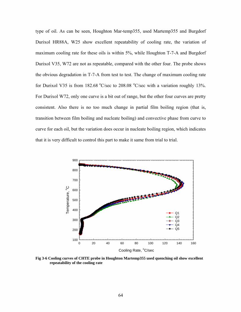
64
type of oil. As can be seen, Houghton Mar-temp355, used Martemp355 and Burgdorf
Durixol HR88A, W25 show excellent repeatability of cooling rate, the variation of
maximum cooling rate for these oils is within 5%, while Houghton T-7-A and Burgdorf
Durixol V35, W72 are not as repeatable, compared with the other four. The probe shows
the obvious degradation in T-7-A from test to test. The change of maximum cooling rate
for Durixol V35 is from 182.68 oC/sec to 208.08 oC/sec with a variation roughly 13%.
For Durixol W72, only one curve is a bit out of range, but the other four curves are pretty
consistent. Also there is no too much change in partial film boiling region (that is,
transition between film boiling and nucleate boiling) and convective phase from curve to
curve for each oil, but the variation does occur in nucleate boiling region, which indicates
that it is very difficult to control this part to make it same from trial to trial.
Cooling Rate, oC/sec
0 20 40 60 80 100 120 140 160
Tem
pera
ture
, o C
100
200
300
400
500
600
700
800
900
Q1Q2Q3Q4Q5
Fig 3-6 Cooling curves of CHTE probe in Houghton Martemp355 used quenching oil show excellent
repeatability of the cooling rate

65
Cooling Rate, oC/sec
0 20 40 60 80 100 120 140
Tem
pera
ture
, o C
100
200
300
400
500
600
700
800
900
Q1Q2Q3Q4Q5
Fig 3-7 Cooling rate curves of CHTE probe in Houghton T7A mineral oil
Cooling Rate, oC/sec
0 20 40 60 80 100 120 140 160
Tem
pera
ture
, o C
100
200
300
400
500
600
700
800
900
Q1Q2Q3Q4Q5
Fig 3-8 Cooling rate of CHTE probe in Houghton Mar-temp 355

66
Cooling Rate, oC/sec
0 20 40 60 80 100 120 140 160 180
Tem
pera
ture
, o C
100
200
300
400
500
600
700
800
900
Q1Q2Q3Q4Q5
Fig 3-9 Cooling rate of CHTE probe in Burgdorf HR88A mineral oil
Cooling Rate, oC/sec
0 50 100 150 200 250
Tem
pera
ture
, o C
100
200
300
400
500
600
700
800
900
Q1Q2Q3Q4Q5
Fig 3-10 Cooing rate of CHTE probe in Burgdorf W72 mineral oil

67
Cooling Rate, oC/sec
0 20 40 60 80 100 120 140 160 180 200 220
Tem
pera
ture
, o C
100
200
300
400
500
600
700
800
900
Q1Q2Q3Q4Q5
Fig 3-11 Cooing rate of CHTE probe in Burgdorf Durixol V35 mineral oil
Cooling Rate, oC/sec
0 20 40 60 80 100 120 140 160 180
Tem
pera
ture
, o C
100
200
300
400
500
600
700
800
900
Q1Q2Q3Q4Q5
Fig 3-12 Cooing rate of CHTE probe in Burgdorf Durixol W25 mineral oil

68
Quenchant Performance Indices: Tamura’s V and HP
Viscosity, mm2/sec
0 20 40 60 80 100 120 140
HP
200
400
600
800
1000
1200
1400
1600
Tam
ura'
s V
2
4
6
8
10
HPTamura's V Regression line for HPRegression line for Tamura's V
Fig 3-13 Tamura’s V, HP as a function of viscosity estimated using CHTE 4140 probe cooling data
Using the equations that are described in sections 2.7.1 and 2.7.2, Tamura’s V and
Hardening Power have been calculated for each experiment, averaged on five values to
get one data point for each type of oil, and then plotted as a function of viscosity of
mineral oil, as shown in figure 3-13. Tcp and Tvp values in equations 2.7.1-1 and 2.7.2-1
are taken from cooling rate-time curve, Tvp is the temperature corresponding to the point
where cooling rate starts to change very sharply within a few seconds at the beginning of
quenching process. Tcp is the temperature that corresponds to the point where cooling
rate starts to approximate a constant value as time goes on at the end of quenching
process. Ts and Tf in equation 2.7.1-1 are respectively 337.78oC and 218.33 oC. In
equation 2.7.2-1 the cooling rate at 550oC is used for CR since the region between 500oC
and 600oC is very critical to understand the quenching process. Figure 3-13 shows the
quenchant performance in the form of HP and V indices. As viscosity increases,
Tamura’s V is nearly constant, while the HP decreases.

69
Effect of operating temperature on the quenching performance of mineral oils
Cooling Rate, oC/sec
0 20 40 60 80 100 120 140
Tem
pera
ture
, o C
100
200
300
400
500
600
700
800
900
25oC 40oC 60oC 80oC
Fig 3-14 Cooling rate curves of CHTE 4140 quenched in Burgdorf HR88A at different temperatures
In order to understand the effect of operation temperature on the quenching performance
of mineral oil, one relatively stable oil (Burgdorf Durixol HR88A) was chosen to test at
25, 40, 60 and 80oC. The results are shown in figure 3-14. Generally as oil is heated
viscosity decreases. [1] This drop in viscosity allows the quenchant to flow more freely to
increase the natural or mechanical turbulence that breaks down the vapor blanket stage.
[1] The boiling stage (i.e. nucleate boiling) is violent by nature and it is not significantly
affected by changes in temperature. In the convection stage, the rate of cooling of an oil
quenchant will become slower as the temperature of the quenching oil bath increases.
From figure 3-14, the cooling curve at 25oC shows the lowest maximum cooling rate, as
the temperature rises up to 40 and 60oC, the maximum cooling rate increases by roughly
20oC/sec. However, as the temperature increases further up to 80oC, the cooling rate
decreases instead. It is assumed that the cooling ability for this type of oil has an upper

70
limit at certain temperature, in this case, which is around 60oC. Below and above this
temperature, the cooling rate is more or less lower.
Effect of probe size
Figure 3-15 shows the cooling rate curves of CHTE 4140 probes with two different
diameters quenched in Burgdorf Durixol W72. The diameter of bigger probe is four times
of the small one, the maximum cooling rate of the larger probe is almost one fourth of
that of the small one.
Cooling rate, oC/sec
0 50 100 150 200 250
Tem
pera
ture
, o C
100
200
300
400
500
600
700
800
900
3/8" diameter1.5" diameter
Fig 3-15 Cooling curves of CHTE 4140 probes with different diameters quenched in Burgdorf W72

71
Heat transfer coefficients of CHTE 4140 steel probe in different mineral oils
Temperature, oC
0 200 400 600 800 1000
Hea
t tra
nsfe
r coe
ffic
ient
, W/m
2 *K
0
500
1000
1500
2000
2500
3000
3500
V35W72 HoughtonG T7A W25 Mar355 HR88A
Fig 3-16 Typical heat transfer coefficient curves of CHTE 4140 steel probe as a function of
temperature quenched in different mineral oils.
Heat transfer coefficients of CHTE 4140 steel probe quenched in seven mineral oils were
calculated using lumped parameter analysis since the probe in our test is tiny, and the
results are shown in figure 3-16. Heat transfer coefficient is similar in partial film boiling
region, but quite different in nucleate boiling and convection stages and its maximum
value varies from 1900W/m2*K up to 3250W/m2*K, Durixol V35 and W72 have the
highest maximum heat transfer coefficients (hmax) and lowest viscosities by which they
are classified as very fast and fast oils, while T7A has lowest hmax and average viscosity.
The other five heat transfer coefficients lay in between. From the point of view of the
viscosity, the lower the viscosity of an oil is, the more easily the bubbles can form on the
probe surface to extract heat, and the higher heat transfer coefficient will be. The
temperature at which maximum heat transfer coefficient reaches differs from oil to oil,
but it is within the band of 640 oC and 720oC.

72
CRmax, oC/sec
100 120 140 160 180 200 220
h max
, w/m
2 *k
1000
1500
2000
2500
3000
3500
Hardening Power
600 800 1000 1200 1400
CRmax vs hmaxHP vs hmaxRegression line for h-CRRegression line for h-HP
Fig 3-17 Heat transfer coefficient as a function of HP and CRmax for CHTE 4140 steel probe in different mineral oils
Heat transfer coefficient of CHTE 4140 steel probe quenched in different mineral oils is
plotted as a function of Hardening power and maximum cooling rate and the curves are
shown in figure 3-20. Polynomial 3rd order regression lines are added onto two sets of
scattered data points. From the trendlines, it can be clearly seen that heat transfer
coefficient increases as the increase of hardening power and maximum cooling rate,
which means that the oil with higher cooling rate has the higher heat transfer coefficient
and better cooling ability, therefore can extract the heat from the probe surface faster and
more efficiently.
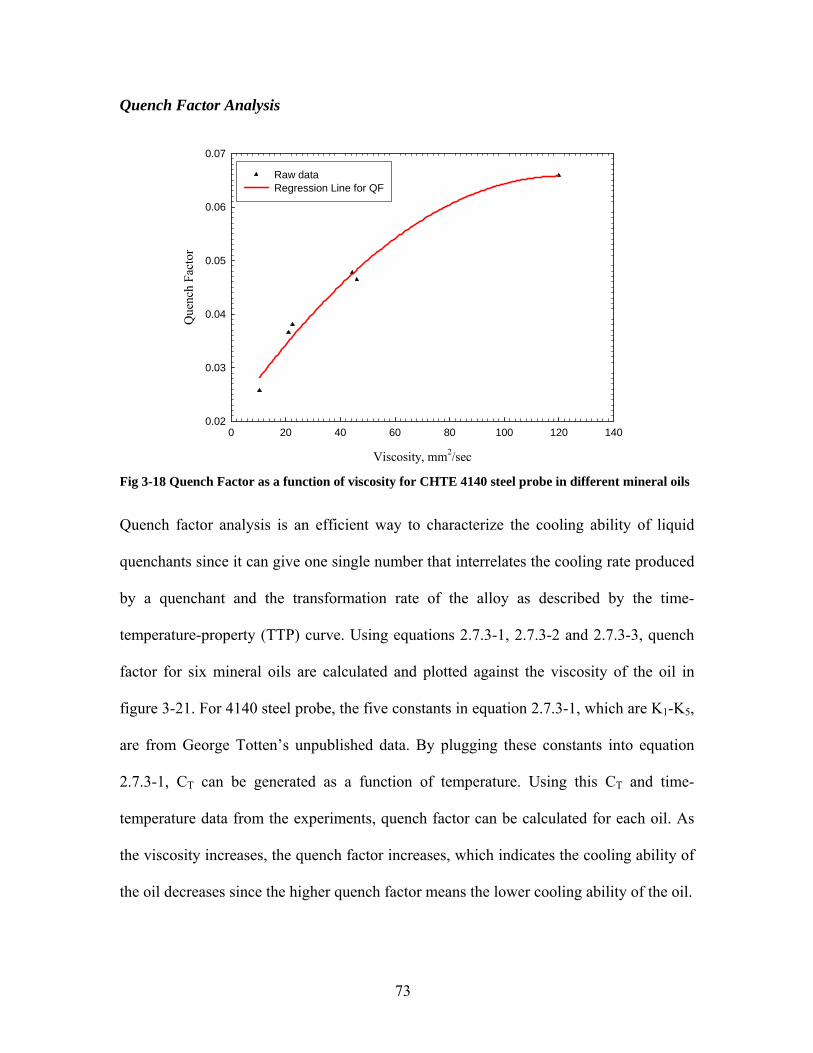
73
Quench Factor Analysis
Viscosity, mm2/sec
0 20 40 60 80 100 120 140
Que
nch
Fact
or
0.02
0.03
0.04
0.05
0.06
0.07
Raw dataRegression Line for QF
Fig 3-18 Quench Factor as a function of viscosity for CHTE 4140 steel probe in different mineral oils
Quench factor analysis is an efficient way to characterize the cooling ability of liquid
quenchants since it can give one single number that interrelates the cooling rate produced
by a quenchant and the transformation rate of the alloy as described by the time-
temperature-property (TTP) curve. Using equations 2.7.3-1, 2.7.3-2 and 2.7.3-3, quench
factor for six mineral oils are calculated and plotted against the viscosity of the oil in
figure 3-21. For 4140 steel probe, the five constants in equation 2.7.3-1, which are K1-K5,
are from George Totten’s unpublished data. By plugging these constants into equation
2.7.3-1, CT can be generated as a function of temperature. Using this CT and time-
temperature data from the experiments, quench factor can be calculated for each oil. As
the viscosity increases, the quench factor increases, which indicates the cooling ability of
the oil decreases since the higher quench factor means the lower cooling ability of the oil.

74
Quench Factor
0.03 0.04 0.05 0.06 0.07
Vic
kers
Har
dnes
s (H
V)
685
690
695
700
705
710
715
720
725
H-QFRegression Line for H-QF
Fig 3-19 Hardness as a function of quench factor for CHTE 4140 steel probe quenched in Houghton
G, T7A and Durixol HR88A
Three probe tips quenched respectively in Houghton G, T7A and Durixol HR88A were
chosen according to the viscosities of these three oils to do the hardness test. Durixol
HR88A has the highest viscosity among the seven oils we tested; Houghton G has a
relatively low viscosity, while the viscosity of T7A lies in between the other two. First
the sample was cut into half using the alumina blade with coolant flowing to prevent the
phase transformation due to the heat generation during the cutting process, mounted with
the cross-section facing down, grinded and then polished to make the surface smooth
enough for micro hardness test. The hardness measurement was made along the cross-
section of each sample using Vickers hardness tester. Figure 3-22 shows a very good
trend of the change in hardness with the quench factor. The quench factors calculated
from these three oils are pretty small, ranging from 0.03 to 0.07, because the cooling
curves for these oils are far away from ferrite-pearlite transformation starting line. The

75
higher the cooling ability of quenchant is, the smaller the quench factor will be and the
higher the hardness is. So smaller quench factor corresponds to the higher hardness, as
shown in figure 3-22.
IV Summary
In summary, the following conclusion can be made for this study:
• The maximum cooling rate decreases with the increase in viscosity.
• During repeatability tests, not much change in cooling curve is observed in partial
film boiling region (that is, transition between film boiling and nucleate boiling)
and convective phase from one trial to other for each oil, but the variation does
occur in nucleate boiling region, which indicates that it is very difficult to control
this part to make it same from trial to trial.
• As viscosity increases, Tamura’s V doesn’t vary that much, while the HP
decreases.
• Cooling ability of a quenching oil increases with the increase in oil operating
temperature, reaches a maximum and then decreases.
• Heat transfer coefficient increases with the increase in hardening power and
maximum cooling rate. Which means that the oil with higher cooling rate has the
higher heat transfer coefficient and better cooling ability, therefore can extract the
heat from the probe surface faster and more efficiently.
• As the viscosity increases, the quench factor increases, which indicates the
cooling ability of the oil decreases since the higher quench factor means the lower
cooling ability of the oil.

76
Paper II
The effects of surface oxides on the quenching performance of 4140 steel in commercial oils
by
Shuhui Ma, Mohammed Maniruzzaman
and Richard D. Sisson, Jr.
77
4. The Effects of surface oxides on the quenching performance of
4140 steel in commercial mineral oils
Shuhui Ma, Mohammed Maniruzzaman and Richard D. Sisson, Jr.
Center for Heat Treating Excellence, Metal Processing Institute
Materials Science and Engineering Program, Mechanical Engineering Department
Worcester Polytechnic Institute, Worcester, MA 01609, USA
Abstract
The effect of oxide formation on the cooling rate and heat transfer coefficient of CHTE
probes has been experimentally investigated using CHTE Quench Probe System and
probe tips of 4140 and 304 steel. In order to prevent the oxide formation, the argon gas
was purged into the furnace with the constant flow rate at 12.77cm3/min. Lumped
parameter approximation was used to calculate the heat transfer coefficient as a function
of temperature during quenching. The cooling rates and heat transfer coefficients were
compared between 4140/304 probes heated in air and 4140/304 heated in argon. It turns
out that the oxidation increases the cooling rate and heat transfer coefficient of 4140 steel
probes, the cooling rate curve of 4140 steel probe heated in argon shows clear
Leidenfrost temperature, which indicates the use of argon is able to prevent the oxidation.
The oxide layer may require a significant thickness to cause the decrease in heat transfer
coefficient. The quenching performances of 304 stainless steel probes are similar in air
and argon.

78
I Introduction
During the quenching of 4140 steel probes, one thin layer of oxides was found to form on
the surface of the probe. Therefore, the main goals of this work are to experimentally
determine the effect of surface oxides on the cooling rate and heat transfer coefficient.
The effect of oxidation on a test probe is very briefly addressed here. In general,
oxidation is not quantified, it is discussed that oxidation causes the nucleate boiling
regime to start earlier [55]. An experiment to determine the effect of surface roughness
on the rewetting process was performed by Lee and Sheng [1]. During the early test runs,
rewetting velocities showed progressive improvement with time, but then subsequently
remained consistent. These investigations concluded that the effect was due to initial
oxidation of the metal part [1].
The vapor blanket (film boiling) phase will disappear partly or completely when
quenching components with oxidized surfaces. The oxide layer appears to be insulating
and may reduce the cooling rate, which can affect the hardening result [55]. In summary,
oxidation will have the effect of reducing or eliminating the film boiling stage. It creates
an additional source of turbulence that assists in dissipating faster the vapor blanket that
forms in the film boiling stage. Since heat transfer in the film boiling stage is via
conduction and radiation, it is the most inefficient regime from the heat dissipation
capacity standpoint. Oxidation should decrease the heat transfer rate in the nucleate
boiling and convection heat transfer regimes [55].

79
The oxidation layer may act as an insulation layer, however the oxide layer may require a
significant thickness (of the order of 200 microns) to cause the significant change in heat
rate [1]. The oxidation layer may contribute to accelerate the dissipation of the vapor
blanket in the film boiling stage, and cause an earlier initiation of the nucleate boiling
stage. High temperature oxidation may decrease cooling rates if it is prolonged long
enough to provide an insulating effect.
The effect of high temperature oxidation on the quenching behavior of 4140 steel probes
is complex [1]. During oxidation the surface topography and composition will change
dynamically. In addition, during cooling the differential thermal expansion of the oxide
and alloy can lead to cracking and spalling of the oxide which leads to a dynamic change
in surface features As the nucleation site density N/A of surface features that nucleate
bubbles during nucleate boiling controls the heat transfer rate as discussed above, it will
be very difficult to characterize the as-fabricated surface features that will control the
heat transfer.
It is the goal of this paper to experimentally determine the effect of oxidation on the
cooling rate and heat transfer coefficient of CHTE probe tips of 4140 and 304 steel using
CHTE Quench Probe System.

80
II Experimental Procedure
CHTE Quench Probe System
A typical CHTE quench probe system has been shown in figure 3.1, which consists of
notebook PC based data-acquisition system, pneumatic cylinder with air valve, a small
box furnace, 1-L size beaker for quenchant and K-type thermocouple-connecting rod-
coupling-interchangeable probe tip assembly. In this set of experiments the important
modifications were made on the box furnace. In order to achieve the non-oxygen
environment, a stainless steel tube was put all the way through the furnace, held by a
clamp on the top. At the bottom, a side screw was put on the side of the tube to connect
the furnace with the gas tank using the copper wire. The top and bottom of the tube were
respectively sealed with the wool and the ceramic cap to avoid the heat loss and also to
maintain the non-oxygen environment during the experiment. Between the gas tank and
the furnace there is a flow meter to monitor how much gas is flowing into the furnace per
unit time. The dimensions of the probe along with the coupling and the connecting rod
have been shown in figure 3-2.
Materials
The probe tips are made of 4140 steels and 304 stainless steels in this set of experiments.
Both kinds of probes are cylindrical, 9.5mm diameter by 38.1mm length. Medium
surface finish with Ra range of 1.0 to 2.0 µm is used for the test.

81
Three mineral oils, Houghton G, T7A and Burgdorf Durixol HR88A, are chosen for the
test in terms of their viscosities: Houghton G has relatively low viscosity, 22.5 mm2/sec,
Durixol HR88A has the highest viscosity among seven oils we have tested, 120mm2/sec,
the viscosity of T7A lies in between. The experimental plan is given in table 4-1:
Design of experiments
For each oil, as shown in table 4-1, five experiments have been performed using the same
renewed probe to test the repeatability of probes. A new probe has been used for each oil
and has been renewed after each quenching. The probe surface has been cleaned lightly
using 180 grit abrasive papers to make the surface clean and free of prior oxide layer
buildup, and then ultrasonically cleaned in acetone to remove the small pieces of oxides
attached on the surface. Surface roughness was measured using Mahr-Federal
Perthometer PRK before each trial to make sure the surface finish for the same set of
experiments is comparable. Mass and diameter were also measured to determine their
changes after renewing each time. For the oils in table 4-1, two of these oils, T7A and
Houghton G, can be used directly at room temperature, (i.e. 25oC) but Burgdorf Durixol
HR88A must be heated up to 60oC, which is determined by the recommended
temperature range from the oil manufacturer, to achieve its optimum cooling ability.

82
Table 4. 1 Test matrix of 4140 and 304 steel probes in Houghton G, T7A and Durixol HR88A
Probe material Name of oils Viscosity at 40oC Operation temp No of trials Heating environment
Houghton G 22.5 25oC 5
T7A 44.3 25oC 5
Durixol HR88A 120 60oC 5
Heating in air
Houghton G 22.5 25oC 5
T7A 44.3 25oC 5
4140
Steel
Durixol HR88A 120 60oC 5
Heating in argon
Houghton G 22.5 25oC 5
T7A 44.3 25oC 5
Durixol HR88A 120 60oC 5
Heating in air
Houghton G 22.5 25oC 5
T7A 44.3 25oC 5
304
Stainless steel
Durixol HR88A 120 60oC 5
Heating in argon

83
III Experimental Results and Discussion
(A) Repeatability tests
Repeatability of 4140 steel and 304 stainless steel probes in air and argon A series of quenching experiments have been preformed using 4140 steel and 304
stainless steel probes quenched in T7A, Houghton G and Durixol HR88A. The goal of
this work is to identify how the surface oxidation is playing a role in the quenching
performance of different mineral oils. The probes have been heated in two kinds of
environments: air and argon. The main purpose of heating the probes in argon is to
prevent the oxide formation. Figure 4.1-4.10 shows the repeatability tests for CHTE
4140 steel and 304 stainless steel probes respectively heated in air/argon and then
quenched in T7A, Houghton G and Durixol HR88A. Since Durixol HR88A is more
stable than T7A and Houghton G, as can be seen from the graphs, the variation of the
cooling rate curve from trial to trial is smaller for quenching in Durixol HR88A than that
in T7A and Houghton G, but most of the graphs show very good repeatability.
Also repeatability and reproducibility (R&R) studies in air and argon were performed
using 4140 steel probe tips quenched in Houghton G. Two operators made 5 medium-
finish probes each on the same lathe and two different individuals performed the
experiments for one set of R&R study in one of two heating environments (air or argon).
The cooling rate data from 800°C down to 200°C in intervals of 100°C for each of the ten
trials were tabulated as well as the maximum cooling rate and temperature at maximum
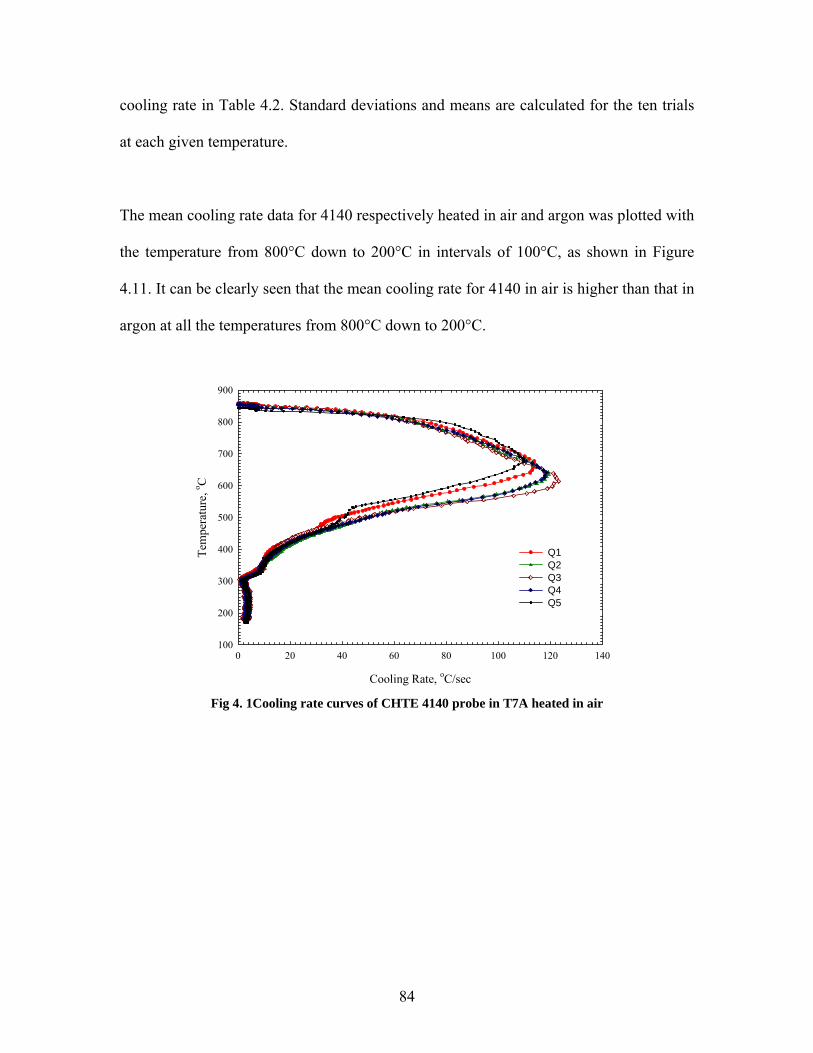
84
cooling rate in Table 4.2. Standard deviations and means are calculated for the ten trials
at each given temperature.
The mean cooling rate data for 4140 respectively heated in air and argon was plotted with
the temperature from 800°C down to 200°C in intervals of 100°C, as shown in Figure
4.11. It can be clearly seen that the mean cooling rate for 4140 in air is higher than that in
argon at all the temperatures from 800°C down to 200°C.
Cooling Rate, oC/sec
0 20 40 60 80 100 120 140
Tem
pera
ture
, o C
100
200
300
400
500
600
700
800
900
Q1Q2Q3Q4Q5
Fig 4. 1Cooling rate curves of CHTE 4140 probe in T7A heated in air

85
Cooling Rate, oC/sec
0 20 40 60 80 100 120 140 160 180 200
Tem
pera
ture
, o C
100
200
300
400
500
600
700
800
900
Q1Q2Q3Q4Q5
Fig 4. 2 Cooling rate curves of CHTE 4140 probe in Houghton G heated in air
Cooling Rate, oC/sec
0 20 40 60 80 100 120 140 160 180
Tem
pera
ture
, o C
100
200
300
400
500
600
700
800
900
Q1Q2Q3Q4Q5
Fig 4. 3 Cooling rate curves of CHTE 4140 probe in DHR88A heated in air

86
Cooling Rate, oC/sec
0 20 40 60 80 100 120
Tem
pera
ture
, o C
100
200
300
400
500
600
700
800
900
Q1Q2Q3Q4
Fig 4.4 Cooling rate curves of CHTE 304 probe in T7A heated in air
Cooling Rate, oC/sec
0 20 40 60 80 100 120 140 160
Tem
pera
ture
, o C
100
200
300
400
500
600
700
800
900
Q1Q2Q3Q4
Fig 4.5 Cooling rate curves of CHTE 304 probe in Houghton G heated in air

87
Cooling Rate, oC/sec
0 20 40 60 80 100 120 140
Tem
pera
ture
, oC
100
200
300
400
500
600
700
800
900
Q1Q2Q3Q4Q5
Fig 4.6 Cooling rate curves of CHTE 304 probe in DHR88A heated in air
Cooling Rate, oC/sec
0 20 40 60 80 100 120
Tem
pera
ture
, o C
100
200
300
400
500
600
700
800
900
Q1Q2Q3Q4Q5
Fig 4.7 Cooling rate curves of CHTE 304 probe in T7A heated in argon

88
Cooling Rate, oC/sec
0 20 40 60 80 100 120 140 160
Tem
pera
ture
, o C
100
200
300
400
500
600
700
800
900
Q1Q2Q3Q4
Fig 4.8 Cooling rate curves of CHTE 304 probe in Houghton G heated in argon
Cooling Rate, oC/sec
0 20 40 60 80 100 120 140 160
Tem
pera
ture
, o C
100
200
300
400
500
600
700
800
900
Q1Q2Q3Q4
Fig 4.9 Cooling rate curves of CHTE 304 probe in DHR88A heated in argon

89
Cooling Rate, oC/sec
0 20 40 60 80 100 120 140 160
Tem
pera
ture
, o C
100
200
300
400
500
600
700
800
900
Q1Q2Q3Q4
Fig 4. 10 Cooling rate curves of CHTE 4140 probe in DHR88A heated in argon
Temperature, oC
100 200 300 400 500 600 700 800 900
Coo
ling
rate
, o C/s
ec
0
20
40
60
80
100
120
140
160
180
With oxidation-in airWithout oxidation-in argon
Fig 4. 11 The comparison of mean cooling rate for 4140 heated in air and argon and quenched in Houghton G as a function of temperature

90
Table 4. 2 R&R Study of 4140 steel probes in Houghton G
R&R in air R&R in Argon
T, oC CRAVG, oC/sec T, oC CRAVG, oC/sec 800 109 800 79.8
705.4 162.7 700 128.8 700 156.1 695.3 129.7 600 128.2 600 108.5 500 72.3 500 60.6 400 30.5 400 22.3 300 5 300 4 200 5.2 200 4.1
(B) Comparison of cooling rate curves
The comparison of cooling rate curves for 4140 in air and in argon
As mentioned before, the five experiments for repeatability test of CHTE 4140 probes
were carried out in each mineral oil. These five curves were then taken average using
high precision polynomial equation or Savitzky-Golay smoothing method, as detailed in
Appendix B, to generate one typical cooling rate curve for the specific mineral oil. The
typical cooling rate curves of CHTE 4140 steel probe tip in air and argon are plotted
together for two different mineral oils: DHR88A and T7A, as shown in figure 4.12 and
4.13.

91
Cooling rate, oC/sec
0 20 40 60 80 100 120 140
Tem
pera
ture
, o C
100
200
300
400
500
600
700
800
900
4140 in air 4140 in argon
Fig 4. 12 Cooling rate curves of CHTE 4140 probes heated in air and argon and quenched in T7A
Cooling rate, oC/sec
0 20 40 60 80 100 120 140 160 180
Tem
pera
ture
, o C
100
200
300
400
500
600
700
800
900
4140 in air 4140 in argon
Fig 4.13 Cooling rate curves of CHTE 4140 probes heated in air and argon and quenched in DHR88A
From figures 4.12 and 4.13, it can be clearly seen that the cooling rate for 4140 in air is
higher than that in argon, which is due to the oxide formation on the probe surface when

92
heating in air that increases surface area, makes the surface rougher and creates more
bubble nucleation sites. Therefore, the bubbles can form more easily and extract more
heat from the surface efficiently. Another interesting observation is that the cooling rate
curve of 4140 probe heated in argon, as shown in figure 4.12, shows clear Leidenfrost
temperature, while the curve of 4140 probe heated in air doesn’t. The apparent reason for
this is that the oxidized surface breaks down the vapor blanket, partially or completely
eliminates the film boiling regime and causes the nucleate boiling stage to initialize
early[55].
The comparison of cooling rate curves for 304 in air and in argon
The same series of experiments were also performed using 304 stainless steel probes,
heated in air/argon and then quenched in three different mineral oils. As can be seen from
figure 4.14, 4.15 and 4.16, the quenching performance for 304 stainless steel probe
heated in argon is quite similar to that in air because for 304 probe tips there is no oxides
formation on the surface even when heated in air. So the result from two kinds of heating
environments should be comparable. Also almost for all the experiments the cooling rate
curves show very prominent Leidenfrost temperature, which is expected to occur.

93
Cooling rate, oC/sec
0 20 40 60 80 100
Tem
pera
ture
, o C
100
200
300
400
500
600
700
800
900
304 in air 304 in argon
Fig 4.14 Cooling rate curves of CHTE 304 probes heated in air/argon and quenched in T7A
Cooling rate, oC/sec
0 20 40 60 80 100 120 140 160
Tem
pera
ture
, o C
100
200
300
400
500
600
700
800
900
304 in air 304 in argon
Fig 4.15 Cooling rate curves of CHTE 304 probes heated in air/argon and quenched in Houghton G

94
Cooling rate, oC/sec
0 20 40 60 80 100 120 140
Tem
pera
ture
, o C
100
200
300
400
500
600
700
800
900
304 in air 304 in argon
Fig 4.16 Cooling rate curves of CHTE 304 probes heated in air and argon and quenched in DHR88A
The comparison of cooling rate curves for 4140 and 304 in air
Cooling rate, oC/sec
0 20 40 60 80 100 120 140
Tem
pera
ture
, o C
100
200
300
400
500
600
700
800
900
4140-T7A304-T7A
Fig 4.17 Cooling rate curves of CHTE 4140 steel and 304 stainless steel probe inT7A in air

95
Cooling rate, oC/sec
0 20 40 60 80 100 120 140 160
Tem
pera
ture
, o C
100
200
300
400
500
600
700
800
900
4140-DHR88A304-DHR88A
Fig 4.18 Cooling rate curves of CHTE 4140 steel and 304 stainless steel probe inDHR88A in air
The comparison of cooling rate curves for 4140 and 304 in argon
Cooling rate, oC/sec
0 20 40 60 80 100 120
Tem
pera
ture
, o C
100
200
300
400
500
600
700
800
900
4140-T7A 304-T7A
Fig 4.19 Cooling rate curves of CHTE 4140 and 304 stainless steel probe inT7A in argon

96
Cooling rate, oC/sec
0 20 40 60 80 100 120 140 160
Tem
pera
ture
, o C
100
200
300
400
500
600
700
800
900
4140-DHR88A304-DHR88A
Fig 4. 20 Cooling rate curves of CHTE 4140 and 304 stainless steel probe in DHR88A in argon
Figure 4.17,4.18,4.19 and 4.20 show the comparison of cooling rate curves between 4140
steel probe and 304 stainless steel probes heated in air/argon and then quenched in T7A
and Durixol HR88A. 304 stainless steel probes show very prominent transition
temperature between film boiling and nucleate boiling stages in each oil and in two kinds
of heating environments. While 4140 steel probes only show this temperature when it is
heated in argon. Also the temperature at which the maximum cooling rate reaches shifts
down from 4140 to 304.
(C) Comparison of heat transfer coefficients As mentioned in section 2.6.6, the specific heat of 4140 steels was modified from the heat
capacity of pure austenitic iron. Also the latest specific heat of 304 stainless steels was
chosen from one of three sources. Using the selected Cp heat transfer coefficient as a

97
function of temperature was calculated for 4140 steel and 304 stainless steel probes in
two kinds of heating environments. Figure 4.21 shows heat transfer coefficients of 4140
steel probe quenched in T7A after respectively heating in air or in argon. Because of the
effect of surface oxidation when heating in air, the maximum heat transfer coefficient in
air shifts to the right side, that is, the higher temperature and also this maximum value is
higher than that in argon, which further confirms that the surface oxides facilitates the
heat dissipation from the probe surface. While it is the different case for 304 stainless
steels, heat transfer coefficients in air and in argon are quite close to each other, as shown
in figure 4.22, since there is no oxidation effect.
Temperature, oC
100 200 300 400 500 600 700 800 900
Hea
t tra
nsfe
r coe
ffic
ient
, W/m
2 *K
0
500
1000
1500
2000
4140-air 4140-argon
Fig 4. 21 Heat transfer coefficients of CHTE 4140 steel probe quenched in T7A

98
Temperature, oC
100 200 300 400 500 600 700 800 900
Hea
t tra
nsfe
r coe
ffic
ient
, W/m
2 *K
0
500
1000
1500
2000
2500
304-air 304-argon
Fig 4. 22 Heat transfer coefficients of CHTE 304 stainless steel probe quenched in T7A
Temperature, oC
100 200 300 400 500 600 700 800 900
Hea
t tra
nsfe
r coe
ffic
ient
, W/m
2 *K
0
500
1000
1500
2000
2500
4140-T7A304-T7A
Fig 4.23 Heat transfer coefficients of CHTE 4140 steel and 304 stainless probe quenched in T7A in air

99
Temperature, oC
100 200 300 400 500 600 700 800 900
Hea
t tra
nsfe
r coe
ffic
ient
, W/m
2 *K
0
500
1000
1500
2000
2500
4140-T7A304-T7A
Fig 4.24 Heat transfer coefficient of CHTE 4140 steel and 304 stainless probe quenched in T7A in Ar
Heat transfer coefficients between 4140 steel and 304 stainless steel probe are also
compared in figure 4.23 and 4.24. It can be seen that the similar maximum heat transfer
coefficients can be achieved even for two completely different materials as long as the
specific heat is properly chosen, but it is almost impossible to obtain the whole curve
with the same shape. When heated in air, the surface oxidation of CHTE 4140 steel probe
completely eliminates the film boiling phase and causes the nucleate boiling stage to
initialize early, so the maximum heat transfer coefficient of 4140 steel probe appears
earlier (that is, at higher temperature) compared with that of 304 stainless steel probe
heated in air. However, when the probes are heated in argon, the temperature at which the
maximum heat transfer coefficient occurs for 4140 and 304 is much closer. For example,
in air the temperatures for 4140 and 304 are respectively 640oC and 560oC, while in
argon they are 570oC and 550oC.

100
(D) Theoretical calculation
If the temperature in the body of cylindrical system can be assumed as a function only of
radial distance and is independent of azimuth angle or axial distance, then we can
examine the applications of Fourier’s Law of heat conduction to calculation of heat flow
in simple one-dimensional system [56].
A different conceptual viewpoint for Fourier’s Law can be introduced. The heat transfer
rate may be considered as a flow and the combination of thermal conductivity, thickness
of material, and area as a resistance to this flow [56]. The temperature is the potential, or
driving, function for the heat flow, and the Fourier equation may be written
Heat flow = thermal potential difference/thermal resistance
a relation quite like Ohm’s law in electric-circuit theory [56]. The one-dimensional heat-
flow equation for the typical heat-flow problem may be written
th
overall
RT
q∑
∆= Eqn. 4.1
Where the Rth are the thermal resistances of the various materials.
In equation 4.1, overallT∆ can be assumed to be constant in our case, so thermal resistance
needs to be determined in order to determine the one-dimensional heat flow. The
convection and conduction are assumed to occur during the quenching process, and then
the thermal resistance for these two kinds of phenomena can be determined.

101
The thermal resistances for the cylindrical probe with and without oxide layer on the
surface can be calculated using the following two equations:
1) With oxide
[ ] )2(2)(21
lrkr
lkr
rrLn
lrrhR
mm
m
o
m
mo
mooth πππ
+
+
++
=Σ Eqn. 4.2
2) Without oxide
)2()2(1
lrkr
lrhR
mm
m
mmth ππ
+=Σ Eqn. 4.3
Where,
ho, hm- heat transfer coefficient of oxide layer and the steel probe
ro, rm- the oxide thickness and the radius of the probe
ko, km – Thermal conductivity of the oxide and the steel probe
l – the length of the steel probe
The heat transfer coefficients of 4140 steels heated in air and argon and then quenched in
Durixol HR88A at 550oC are chosen to do the calculation of the thermal resistances of
4140 steel probes. The results are shown in Table 4.3 and Figure 4.25. The oxide
thickness, ro, used in the calculation is 10,100 and 200µm. Ro and Rm stand for the
thermal resistances of 4140 probes with oxide and without oxide.
Table 4. 3 The variation of thermal resistance of 4140 steels with the oxide thickness
ho=hm=1072.2 W/m2*K ho≠hm ho=1072.2 W/m2*K hm=1354.5 W/m2*K
ro, µm ro/rm Ro/Rm ro/rm Ro/Rm 10 0.0021 1.00132 0.0021 1.23035 100 0.021 1.01322 0.021 1.24498 200 0.042 1.02654 0.042 1.26135
rm
ro

102
ro/rm
0.00 0.01 0.02 0.03 0.04 0.05
Ro/R
m
0.95
1.00
1.05
1.10
1.15
1.20
1.25
1.30
ho=hm=1072.2 W/m2*K
ho=1072.2 W/m2*Khm=1354.5 W/m2*K
Fig 4.25 The variation of thermal resistance of 4140 steels with the oxide thickness
From the calculated results as shown above, the thermal resistances of the 4140 probes
with and without oxide layer show very small difference when the same heat transfer
coefficients of the oxide and the steel probe is used in equations 4.2 and 4.3, which
means the existence of a thin oxide layer on the surface of the probe doesn’t have obvious
effect on the heat transfer between the quenchant and the probe.
J.P.Holman [56] expressed the critical-radius-of-insulation concept. If the outer radius is
less than this critical value, then the heat transfer will be increased by adding more
insulation [56]. For outer radii greater than the critical value an increase in insulation
thickness will cause a decrease in heat transfer. The central concept is that for sufficiently

103
small values of h the convection heat loss may actually increase with the addition of
insulation because of increased surface area [56].
Juan Chaves included the calculation of this critical radius for 4140 steel probes in his
dissertation. In his work, Values of heat transfer coefficient were chosen from actual
experiments [1]. Three values of heat transfer coefficient were chosen. A high value of
3800 watts/m2 K., a middle one 2000 watts/m2-K, and a low of 500 watts/m2-K were
chosen. The highest heat transfer coefficient shows that a 10% variation in heat rate
requires an increase in thickness of about 200 microns [1]. Thus, the surface roughness
effects are more likely to affect the cooling performance. As a result in order for
oxidation to have a significant effect on the heat transfer, it must make a layer over 200
microns thick [1].
From the real quenching experiment, the oxide thickness on the surface of 4140 probe
tips that has been heated to 850oC and held at that temperature respectively for 1 hour and
4 hours was measured to be 78.67µm and 104.0µm, which are much less than the critical
insulation radius 200µm, therefore, in this case the effect of oxide on the quenching
performance of 4140 probe is to increase the cooling rate and heat transfer.

104
IV Summary
In summary, the following conclusions can be made for this study:
For 4140 steel probes, the formation of oxide in air increases the cooling rate
and heat transfer coefficient since the oxidation increases the surface area,
makes the surface rougher and creates more bubble nucleation sites.
The cooling rate curve of 4140 steel probe heated in argon shows clear
Leidenfrost temperature since the existence of oxidized surface can break
down the film boiling phase, partially or completely eliminate the film boiling
regime and cause the nucleate boiling stage to initialize early.
The oxide layer may require a significant thickness to cause the decrease in
heat transfer coefficient.
For 304 stainless steel probes, the cooling rate and heat transfer coefficient are
quite similar in air and in argon.
The similar maximum heat transfer coefficient can be achieved for two
different materials, but it is almost impossible to obtain the whole curve with
the same shape.

105
References
1. Chaves, J.C., The Effect of Surface Condition and High Temperature Oxidation
on Quenching Performance of 4140 Steesl in Mineral Oil, in Manufacturing
Engineering. 2001, Worcester Polytechnic Institute: Worcester. p. 8, 9.29.
2. Totten, G.E., Howes, Maurice A.H, Steel Heat Treatment Handbook, 1997,
Marcel Dekker, Inc. p. 157.
3. Houghton, Houghton On Quenching, Houghton International. Inc.2000. p. 7.
4. C.E.Bates, G.E.Totten. Application of quench factor analysis to predict hardness
under laboratory and production conditions. in The first International Conference
on Quenching & Control of Distortion. 1992. Chicago, Illinois.
5. G.E.Totten, C.E.Bates. N.A.Clinton. Handbook of Quenchants and Quenching
Technology. 1993: ASM International. p62,140-144.
6. Zhou, R.L. 4th Annual conference of heat treatment. 1987. Nanjing: Institute of
Chinese Mechanical Engineering.
7. ISO/DIS 9950, International Organization for Standardization, Industrial cooling
oils-Determination of cooling characteristics-Laboratory Test Method. 1988.
8. Wolfson Heat Treatment Center Engineering Group Specifications, Laboratory
Test for Assessing the Cooling Curve Characteristics of Industrial Quenching
Media. 1982.
9. S. O. Segerberg, Heat Treat, 1988: p. 30-33.
10. R-J, Windgassen, Metalworking Fluid Today, Society of Tribologists and
Lubrication Engineers, 1989.

106
11. P.S. Protsidim, N. Ya. Rudakova, and B.K. Sheremeta. Metalloved. Term. Obrab.
Met, 1988: p. 5-7.
12. H.M. Tensi and P. Stitzelberger-Jakob, Journal of Bedeutungdes H-Wertes
Bestimmung Harteverteilung, 1989. 44: p. 99-105.
13. G. E.Totten, H.M.Tensi and K.Lainer, Performance of vegetable oils as a cooling
medium in comparison to a standard mineral oil. Journal of Materials
Engineering and Performance, 1999. 8(4): p. 409-416.
14. L.A.T.Honary. Performance of vegetable oils as a heat treatment quenchant. in
Second International conference on Quenching and Control of Distortion. 1996.
15. Taekyung Im, 2001, Worcester Polytechnic Institute, MA: Worcester. p. 1-3.
16. M.Tagaya & I.Tamura, Journal of JIM, 1951. 15(11): p. 538-541.
17. M.Tagaya & I.Tamura, Studies on the quenching media: theoretical study of
cooling process during quenching. Journal of JIM, 1951. 15(12): p. 589-594.
18. M.Tagaya & I.Tamura., Studies on the quenching media: The cooling abilities of
water and aqueous liquids. Journal of JIM, 1952. 16(2): p. 107-111.
19. M.Tagaya & I.Tamura, Journal of JIM, 1955. 6(1): p. 7-12.
20. G.E.Totten, K.Funatani. Overview of Prof. Imao Tamura's Contribution to the
field of heat treating. in The second international conference on quenching and
the control of distortion. 1996. cleveland, Ohio.
21. I.Tamura, M.Tagaya, Studies on the quenching media: The cooling ability of
various aqueous liquids. Technology reports of the Osaka University, 1954.
2(47): p. 209-222.

107
22. I.Tamura, M.Tagaya , Studies on the quenching media: The cooling ability of oils.
Technology reports of the Osaka University, 1954. 4(123): p. 305-319.
23. Segerberg, S., Classification of quench oils: a method of comparison. Journal of
Heat Treating, 1988: p. 30-33.
24. Gilliland, H.-J., Journal of Met.Prog., 1960: p. 111-114.
25. E.A.Bender, H-J. Gilliland, Journal of Steel, 1957: p. 56-59.
26. C.A.Barley, J.S.Aarons, The lubrication Engineers Manual. 1971, U.S. Steel
Corp. p. 56-57.
27. W. E. Jominy, Hardenability of Alloys Steels. American Society for Metals, 1939:
p. 73.
28. IVF, IVF quenchotest. 2000: Sweden.
29. Instruments and Technology Inc, Quenchalyzer. 2000.
30. M. Tagaya and I. Tamura, Journal of Hart.-Tech. Mitt., 1963. 18: p. 63-67.
31. I.Tamura, N. Shimizu, and T. Okadu, Journal of Heat Treating, 1984. 3: p. 335.
32. American Society for Metals., ed. Metals Handbook. 9th ed. Vol. 4. 1981. p32-35.
33. R.F.Price and A.J.Fletcher, Journal of Met. Technology., 1980: p. 203-211.
34. Liscic, B., Journal of Hart.-Tech. Mitt., 1978. 33: p. 179-191.
35. K. E. Thelning, Journal of Scand. J. Metall., 1983. 12: p. 189-194.
36. J.R.Davis, Metals Handbook. 1990: ASM International. p. 197-199, 203.
37. Smith, William F., Structure and Properties of Engineering Alloys. 2nd ed. 1993,
New York: McGraw Hill. p.156.

108
38. Paul M. Unterweiser, Howard E. Boyer, James J. Kubbs, ed. Heat treater's guide:
standard practices and procedures for steel. 1982, American Society for Metals:
Metals Park, Ohio.
39. Donald Peckner, I. M. Bernstein, Handbook of Stainless Steels, ed. B.G. Harold
B.Crawford. 1977, New York: McGraw-Hill Book Company. p.4-10,4-11.
40. Callister, William D, Materials Science and Engineering: An Introduction. 5th
Edition ed, Wayne Anderson, ed. 2000, New York: John Wiley & Sons Inc. p.
659, 664.
41. Y.S.Touloukian, Thermophysical properties of matter. TPRC data series. Vol. 1.
1970, NY: IFI Plenum. p.1154-1156,1160-1175.
42. Y.S.Touloukian, E.H.Buyco., Thermophysical Properties of Matter. TPRC data
series. Vol. 4. 1970, NY: IFI Plenum. p.699-701.
43. M.F.Rothman, ed. High-Temperature Property Data: Ferrous Alloys. 1988, ASM
International: Metals park, OH. p.9.27.
44. Kohlhaas, R. Braun, M, Journal of Archiv. fur das Eisenhuttenwesen, 1963. 34(5):
p. 391-399.
45. Sciance, C.T., C.P. Colver, and C.M. Sliepcevich, Film Boiling Measurements
and Correlations for Liquified Hydrocarbon Gases. Journal of Chem. Eng. Prog.
Symp. Ser, 1967.
46. Bromley, L.A., Heat Transfer in Stable Film Boiling. Journal of Chem. Eng. Prog,
1950. 46: p. 221.
47. Hsu, Y.Y. and J.W. Westwater, Approx. Theory for Film Boiling on Vertical
Surfaces. Journal of AIChE Chem Eng. Prog. Symp. Ser, 1960.

109
48. Benjamin, R.J. and A.R. Balakrishnan, Nucleate pool boiling heat transfer of pure
liquids at low to moderate heat fluxes. Int. J. Heat Mass Transfer, 1996. 39 (12).
49. Benjamin, R.J. and A.R. Balakrishnan, Nucleation Site Density in Pool Boiling of
Saturated Pure Liquids:Effect of Surface Microroughness and Surface and Liquid
Physical Properties. Experimental Thermal and Fluid Science, 1997. V15.
50. McAdams, W.H., Heat Transmission. 3rd ed. 1945, New York: McGraw-Hill.
51. Churchill, S.W., Free Convection around Immersed Bodies, in Heat Exchanger
Design Handbook. 1983, Hamisphere Publishing Co.
52. A.F.Mills, Heat Transfer. 2nd ed. 1999, Upper Saddle River, NJ: Prentice Hall
Inc. p.29-31.
53. Segerberg, Soren, and Bodin, Jan, Controlling the quench process for more
consistent hardening. Heat Treating, 1988: p. 26-28.
54. C.E.Bates, G.E.Totten, Quench severity effects on the As-quenched hardness of
selected alloy steels. Heat Treatment of Metals, 1992. 2: p. 45-48.
55. Segerberg, Soren, and Bodin, Jan. Correlation between characteristics of
quenching media and hardness distribution in steel. in Heat treatment. 1984.
London, England: The Metals Society.
56. J.P.Holman, Heat Transfer. 8th edition. J.M. Debra Riegert, editor. 1997:
Publication Services, Inc. p.26-38.


A-1
APPENDIX A
CHTE QUENCH PROBE SYSTEM

A-2
CHTE QUENCH PROBE SYSTEM
A.1 General Description A typical CHTE Quench Probe System is shown in Fig. C.1. The system
consists of notebook PC based data-acquisition system, pneumatic cylinder
with air valve, a small box furnace, 1-L size beaker for quenchant and K-type
thermocouple-connecting rod-coupling-interchangeable probe tip assembly.
The pneumatic cylinder rod moves the probe down into the quench tank from
the box furnace. The pneumatic cylinder is connected to the pneumatic valve
by two white tubes as shown.
Probe tip-coupling-connecting rod assembly
The probe is cylindrical in shape in order to enable ease of heat transfer
calculation using 1-D approximation. The dimensions of the probe along with
the coupling and the connecting rod are shown in Fig. C.2. In the present
study a cold drawn annealed 4140 steel has been selected. The 4140 steel
was selected is because widely used in industry. The probe tip is connected to
the pneumatic cylinder by a steel coupling and a stainless steel connecting
rod. A glass mica heat insulator of 17 mm in dia and 25 mm in length joins
the connecting rod with the pneumatic cylinder by an internal thread on the
mica ceramic of size 7.94 mm and 24 threads per 25.4 mm (5.16”-24). An
Allen setscrew of 1.59 mm (#6-32) is used in the coupling to secure the
thermocouple in position.

A-3
Pneumatic cylinder
Furnace
Oil beaker
Hydraulic on/off switch
K-type thermocouple
Probe tip
Connecting rodComputer with Data
Acquisition Card
Thermocouple for Oil temp.
Fig. A.1 CHTE Quench Probe System

A-4
3/8"
1 1/2" 2 1/2" 14"
Probe TipCoupling Connecting rod
1/16" allen set screw#6 - 32 threads per in.
K-typeThermocouple
20 threads per inch1/4" L- 1/4" D
24 threads per inch1/4" L- 5/16" D
3/4"
Fig. A.2 CHTE probe-coupling-connecting rod assembly
Pneumatic system
The quenching system has a pneumatic cylinder to push the probe tip
into the quench tank from the furnace. The cylinder is connected with the air
supply line through a pressure regulator and a pneumatic release valve. The
switch on the release valve controls the up and down motion of the connecting
rod. The mica coupling between the pneumatic cylinder and the connecting
rod activates a trigger switch on its way down in order to initiate the data
acquisition. The cylinder is stainless steel of size 405mm. The probe tip is
heated in the furnace and is pushed down into the oil with an air pressure of
35 psi. Furnace-with temperature controller
A small benchtop muffle furnace1 of 76 cubic inch chamber size is used
in the CHTE Quench System. The furnace has on off temperature control.
The furnace is placed by putting its door face up and a through hole has been
drilled in order to allow the probe to transfer from the furnace to the quench
tank. Quench tank
For experiment without agitation, a 1-litter glass beaker is used as a quench
tank. For this work a 1-litter beaker is sufficient given the mass of the probe
tip. 1 Thermolyne small benchtop muffle furnace (Model no. FB1315M: Operating temp. 100-1100oC, power 1050 watts), Barnstead | Thermolyne, 2555 Kerper Boulevard, Dubuque, Iowa USA 52001-1478

A-5
Thermocouple connection
A 1.59mm dia and 609.6mm long K type thermocouple2 with inconel 600
sheaths is used for time-temperature data recording. The thermocouple is
inserted through a side hole at the upper end of the connecting rod. In order
to attain a better contact between the probe tip and the thermocouple, a
small amount of graphite powder is used. A second thermocouple is used to
record the quench oil temperature. Data acquisition
Time-temperature data from the thermocouple placed at the center of the
probe is acquired using LabView Data Acquisition software3 on a notebook
computer running windows 98. The thermocouple is connected to a connector
box, which is connected to the computer via PCMCIA DAQCard and a cable.
The connector box can accommodate maximum 15 thermocouple connections.
The data analysis and graphing is done using Microsoft Excel and
SIGMAPLOT graphing software. The DAQCard is capable of sampling rate
of 20kS/sec (20000 samples/second) single channel with 16 bit resolution.
2 OMEGA Engineering, INC. One Omega Drive, Stamford, Connecticut 06907-0047, P.O. Box 4047, (800)-848-4286 or (203)-359-1660, http://www.omega.com 3 National Instruments Corporation, 11500 N Mopac Expwy, Austin, TX 78759-3504, 512-794-0100, http://www.ni.com

A-6
A.2 Operating procedure of the CHTE Quench Probe
System
Fig. A.3 Virtual Instrument panel for data acquisition used for CHTE Quench
Probe System
1. Insert the Data Acquisition Card into the computer and then connect
computer with experimental set-up through a connector box.
2. Put a little bit graphite inside the probe tip to make sure the good
contact between thermocouple and the probe tip.
3. Fix the connecting rod to the ceramic part at the end of pneumatic
cylinder, bring the connecting rod down using the hydraulic on/off
switch, connect the coupling with the rod underneath the table, insert
the K-type thermocouple all the way through the connecting rod and
the coupling from the side hole of the connecting rod, connect the probe
tip and the coupling, fasten the thermocouple using the side set screw
on the coupling (the probe tip and the coupling need to be made of the
same materials to make sure their thermal expansion is the same).

A-7
4. Bring the connecting rod up and connect the thermocouple with the
connector box.
5. Start the LabView Virtual Instrument (VI) Panel Quenching.vi, shown
in fig. A.3, input the name of the thermocouple channel being used for
data acquisition under the channels (one for measuring the probe
temperature, the other for measuring the oil temperature, such as TC1
& TC2) and the scan rate (i.e 5 scans/second). Start the VI by selecting
operate run. The VI will ask for a filename to store the time-
temperature data. At this point VI will not acquire any data. A
trigger switch located on the pneumatic cylinder panel starts the data
acquisition by the downward movement of the probe.
6. Turn on the furnace and set the target temperature to 850oC. To
monitor the probe temperature, start the data acquisition by lowering
the probe slightly down and then up using the hydraulic on-off lever.
When the thermocouple temperature reaches 845 ºC, stop running the
program by pressing stop button on the VI. Change the scan rate to
1000 scans/second, start the VI by selecting operate run, give the file
name. Hold the probe at this temperature for 5 minutes to make sure
it transforms into austenite completely.
7. Put 1-Liter beaker with quenchant inside (i.e mineral oil, water etc.)
under the table, after 5 minutes, bring the probe down into the
quenchant by putting the hydraulic on-off lever at lower position. Data
acquisition will start automatically.
8. When the recorded data are up to about 60,000, which can be seen
from the VI panel, stop the data acquisition.
9. Remove the probe tip from the end of the coupling, replace with
another one, and then the system is ready for next quenching.

B-1
APPENDIX B
EXPERIMENTAL DATA SMOOTHING

B-2
EXPERIMENTAL DATA SMOOTHING In our quenching test, minimum five experiments were performed to test the repeatability
of probe for each of seven mineral oils. For each experiment, roughly 60,000 data points
were collected with data scan rate 1000 readings/second using notebook PC based data-
acquisition system, as detailed in Appendix A. This sampling rate is well within the
capability of the DAQCard-A1-16XE-50 National Instruments data acquisition card. The
card has a sampling rate of 20kscans/second and a sixteen-bit resolution. It was
combined with a SCCB 68 connector box with cold junction compensation and
connectors for 15 thermocouples. After time-temperature data are obtained, how to
process so huge data to eliminate the noises without any loss of important information is
always our concern.
One popular way to do this is the moving average method. The data smoothing can be
done by a running average with SigmaPlot. The number of points used in the running
average is 60 or slightly different depending on the size of the original file. This number
is calculated using a sampling proportion of 0.001. The sampling proportion is the
fraction of the total number of data points used to compute each smoothed value. As a
result the number of points in the smoothed and reduced data file is 1000, or slightly
different depending on the size of the original file. Using the reduced data points of time-
temperature, the first derivative dT/dt can be calculated using the user-defined
transformation in SigmaPlot as given below. Figure B-1 shows an example of data
smoothing with SigmaPlot – cooling and cooling rate curves of CHTE 4140 steel probe
quenched in Durixol V35, which give a very clear picture of what is going on during the

B-3
whole quenching process. The maximum cooling rate, the temperature at which this
maximum cooling rate reaches and the time that is needed to reach certain cooling rate
can be read directly from the graph, which is very essential and useful to understand the
quenching process.
**** Computation of Derivatives **** This transform takes an t, T data set with increasing ordered t values and computes the first and second derivatives. ********** Input Variables ********** Cx=1; t data column number Cy=5; T data column number ************ RESULTS ************ The results are placed into a block of 3 columns starting at column cr. Columns cr to cr+2 contain the first two derivatives. Column cr+3 is for working variables. Cr=6; 1st column of results block ************ PROGRAM ************ Cr1=cr Cr2=cr+1 Cr3=cr+20; working column n=size(col(cx)) Cell (cr3, 1)=cx Cell (cr3, 2)=Cy Cell (cr3, 3)=cr Compute first derivative for 3 to n-2 rows nm1=n-1 nm2=n-2 Cell (cr3, 4)=cell (cx, 2)-cell (cx, 1); dt1 Cell (cr3, 5)=(cell (cy, 2)-cell (cy, 1))/cell (cr3, 4); dT1 Cell (cr1, 1)=cell (cr3, 5) Cell (cr1, 2)=cell (cr3, 5) dt2=-12*cell (cr3,4) ;dt2 For i=3 to nm2 do dT2=(cell(cy,i-2)-8*cell(cy,i-1)+8*cell(cy,i+1)-cell(cy,i+2))/dt2 Cell (cr1, i)=dT2 End for Cell (cr1, nm1)=(cell (cy, n)-cell (cy, 1))/cell (cr3, 4)*6 Cell (cr1, n)=cell (cr1, nm1)

B-4
Fig B- 1 Sample of data smoothing using moving average method– cooling and cooling rate curves of CHTE 4140 steel probe in Durixol V35 The moving average method mentioned above is only for reducing the data points upon
the condition that no important information is lost and for smoothing the individual curve
for each experiment. While in the repeatability test one typical curve needs to be
generated from five experiments for the same probe to represent the quenching
performance of specific probe in specific quenchant. Table Curve 2D 5.0 is a powerful
tool to do the linear and non-linear automated curve fitting. First the raw data of T-dT/dt
need to be stored in two columns as the formats of either excel spreadsheet, or SigmaPlot
file, or ASCII text, then imported or opened in Table Curve editor window. All kinds of
equations can be chosen to fit the data. In our case two methods were utilized: high
precision polynomial equation and Savitzky-Golay smoothing.
Time, sec
0 10 20 30 40 50 60
Tem
pera
ture
, o C
100
200
300
400
500
600
700
800
900
Cooling Rate, oC/sec
0 50 100 150 200 250
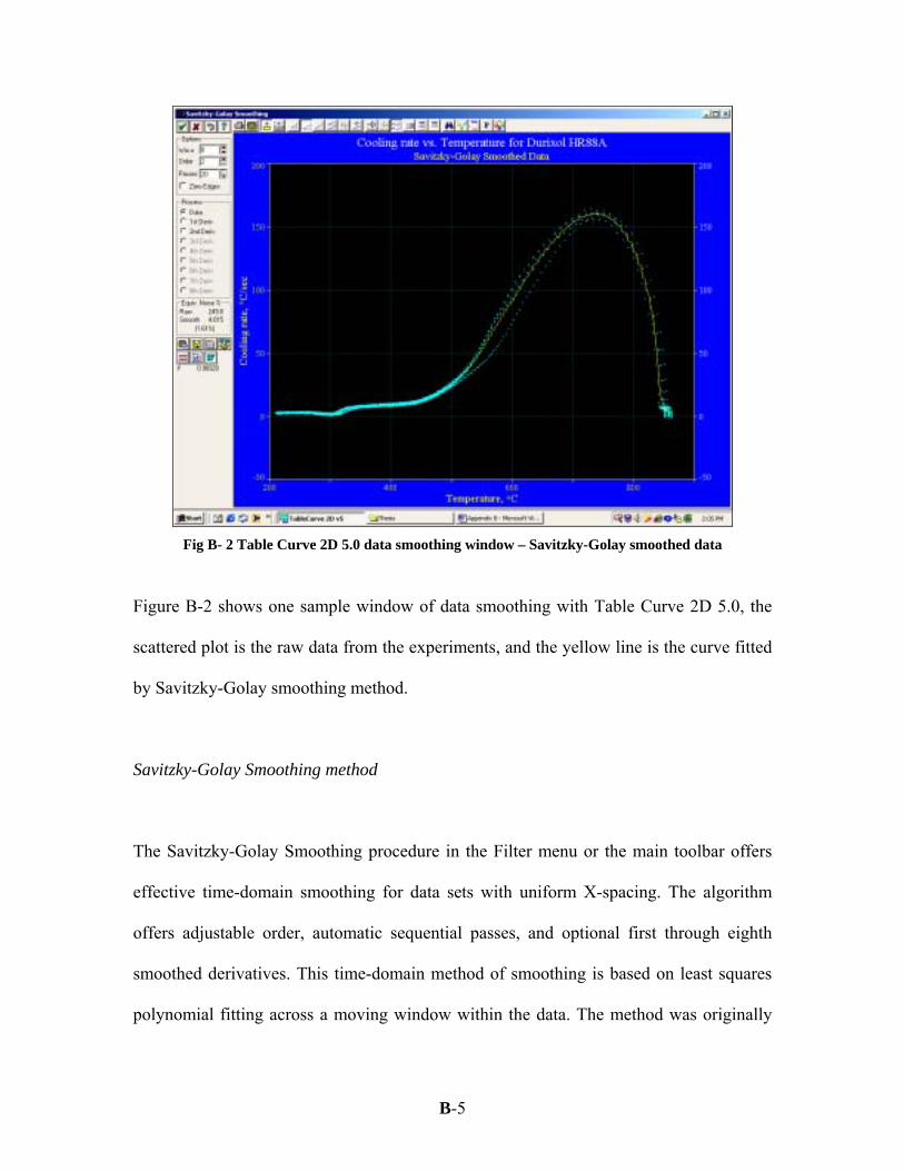
B-5
Fig B- 2 Table Curve 2D 5.0 data smoothing window – Savitzky-Golay smoothed data
Figure B-2 shows one sample window of data smoothing with Table Curve 2D 5.0, the
scattered plot is the raw data from the experiments, and the yellow line is the curve fitted
by Savitzky-Golay smoothing method.
Savitzky-Golay Smoothing method
The Savitzky-Golay Smoothing procedure in the Filter menu or the main toolbar offers
effective time-domain smoothing for data sets with uniform X-spacing. The algorithm
offers adjustable order, automatic sequential passes, and optional first through eighth
smoothed derivatives. This time-domain method of smoothing is based on least squares
polynomial fitting across a moving window within the data. The method was originally

B-6
designed to preserve the higher moments within time-domain spectral peak data. The
TableCurve 2D implementation of the Savitzky-Golay algorithm offers sequential
internal smoothing passes to improve overall noise reduction. The fitted curve by
Savitzky-Golay smoothing method and raw data are given in figure B-3.
Fig B- 3 Savitzky-Golay smoothed cooling rate-temperature data –CHTE 4140 steel probe in HR88A
High Precision Polynomial Smoothing method
TableCurve 2D 5.0 provides high precision polynomial equations from 4th order through
20th order, which has such standard format as Y=a+bx+cx2+dx3+…. One of the
advantages of this smoothing method is not only the fitted data but also the prediction
limits and confidence limits can be obtained directly from the smoothing result.
Confidence intervals indicate how accurately the fitted curve can be achieved using
TableCurve; a 99% confidence interval is the Y-range for a given X that has a 99%
0
50
100
150
200
100 200 300 400 500 600 700 800 900
Temperature, oC
Coo
ling
rate
, o C/s
ec
Raw data
SG smoothed data

B-7
probability for containing the true Y value. While Prediction intervals are useful for
predicting, for a given X, the Y value of the next experiment. It is often used when a fit
represents a single experiment, where each Y value is a single observation rather than an
average. In this case, the weight for each Y value isn't based upon a standard deviation
from multiple observations, but rather is inversely related to the experimental uncertainty
for the individual measurement, if such is known. If the uncertainty of the Y
measurement is unknown or thought to be equal for all X, all points can use equal 1.0
weight.
Fig B- 4 Sample of data smoothing using High Precision Polynomial Equation A 99% prediction interval is the Y range for a given X where there is a 99% probability
that the next experiment's Y value will occur, based upon the fit of the present
experiment's data. Figure B-4 is a sample graph with 99% confidence and prediction
limits. The data are generated using high precision polynomial smoothing method.
0
50
100
150
200
100 200 300 400 500 600 700 800 900
Temperature, oC
Coo
ling
Rat
e, o C
/sec
Average of raw data99% prediction lower limit99% prediction upper limitRaw data99% confidence lower limit99% confidence upper limit

B-8
Therefore, the experimental results can be presented as the average curve with the
confidence and prediction limit bands instead of five individual curves.
Fig B- 5 Comparison of two different smoothing methods –CHTE4140 steel probe in Durixol HR88A
Two different ways of data smoothing are compared in figure B-5. It can be clearly seen
that two lines are very close to each other. Which one to use in practice depends on the
specific requirement and condition.
0
50
100
150
200
100 200 300 400 500 600 700 800 900
Temperature, oC
Coo
ling
Rat
e, o
C/s
ec
Raw dataPolynomial regression lineSG Regression line