characterization and modeling of a flexible matrix
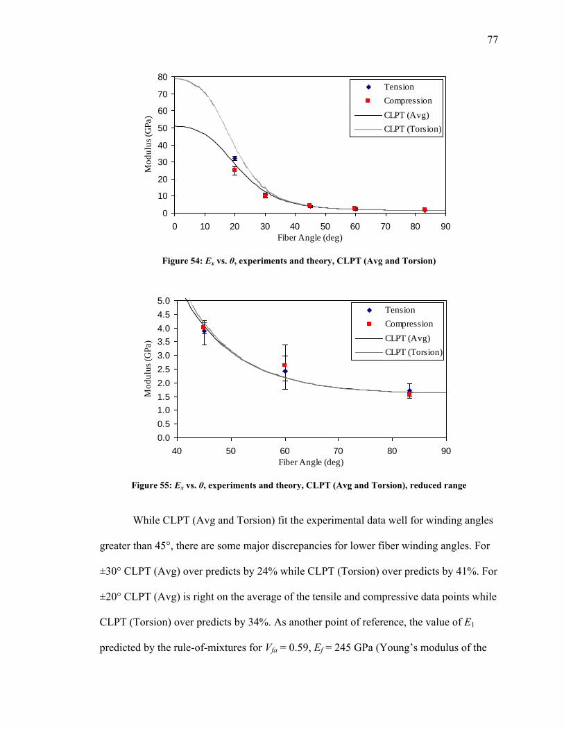
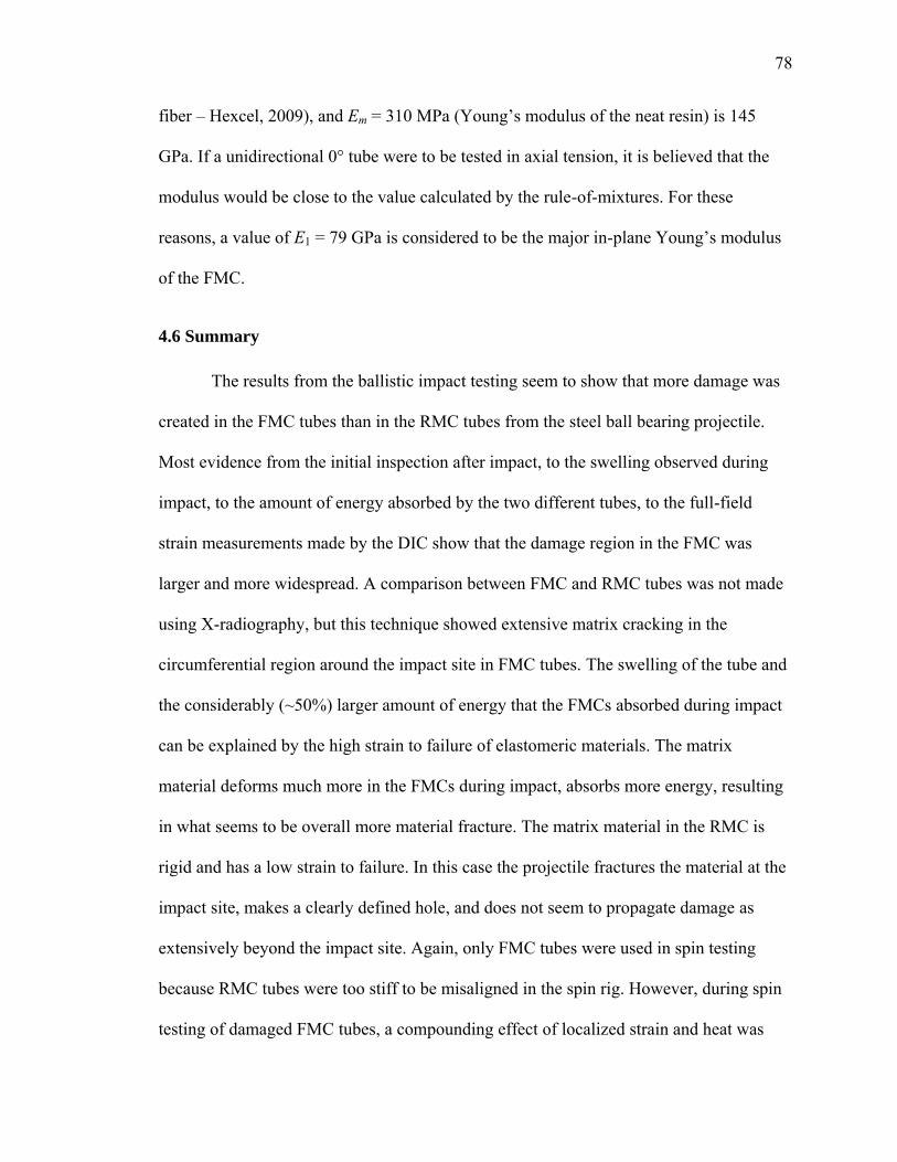
TRANSCRIPT
The Pennsylvania State University
The Graduate School
Department of Engineering Science and Mechanics
CHARACTERIZATION AND MODELING OF A FLEXIBLE MATRIX
COMPOSITE MATERIAL FOR ADVANCED ROTORCRAFT DRIVELINES
A Thesis in
Engineering Mechanics
by
Stanton G Sollenberger
2010 Stanton G Sollenberger
Submitted in Partial Fulfillment
of the Requirements
for the Degree of
Master of Science
August 2010
ii
The thesis of Stanton G Sollenberger was reviewed and approved by the following
Charles E Bakis
Distinguished Professor of Engineering Science and Mechanics
Thesis Advisor
Edward C Smith
Professor of Aerospace Engineering
Renata S Engel
Professor of Engineering Science and Mechanics
Judith A Todd
P B Breneman Department Head Chair
Professor Department of Engineering Science and Mechanics
Signatures are on file in the Graduate School
iii
ABSTRACT
Most of the current driveline designs for rotory wing aircraft (rotorcraft) consist
of rigid aluminum shafts joined by flexible mechanical couplings to account for
misalignment in the driveline The couplings are heavy and incur maintenance and cost
penalties because these parts wear and need frequent replacement A possible solution is
to replace the current design with a continuous flexurally-soft torsionally-stiff flexible
matrix composite (FMC) shaft This design could eliminate the flexible couplings and
reduce the overall weight of the driveline Previous research studies on this topic using
preliminary materials have found design solutions that meet operational criteria
however these designs employed thick-walled heavy shafts In order to significantly
reduce the weight of the driveline a stiffer FMC material resulting in a lighter shaft
design is required A new FMC with a matrix material that is stiffer than the previous
preliminary material by a factor of five is characterized in this thesis It is believed that
future design solutions with this new material will increase weight savings on the final
driveline design
For rotorcraft operated in hostile environments a topic of concern regarding FMC
shafts is ballistic impact tolerance This topic has not yet been explored for these new
kinds of composite materials and is pursued here on a coupon-level basis Results show
that tubular FMC test coupons absorb more energy and suffer larger reductions in
torsional strength than their conventional composite counterpart although reductions in
tensile and compressive strengths are similar in both materials This difference is
attributed to the greater pull-out of fibers in the FMC material Coupon-level testing is a
good first step in understanding ballistic tolerance in FMCs although additional testing
iv
using fully sized and designed shafts is suggested so that proper comparisons between
driveshafts can be made
Self-heating of FMC shafts is an important issue because many design criteria are
dependent on temperature A model has already been developed to simulate self-heating
in FMC shafts although it is limited to analyzing composite layups with one fiber angle
and no ballistic damage New closed-form and finite element models are developed in the
current investigation that are capable of analyzing self-heating in FMC shafts with
multiple fiber angles through the thickness The newly developed models have been
validated with comparisons against experiments and one another Experiments using
simple angle-ply tubes made with the new FMC suggest that for a shaft operating under
real service strains temperature increase due to self-heating can be less than 10degC
Material development characterization of the ballistic tolerance of FMCs and improved
analytical tools are contributions from the current investigation to the implementation of
FMC driveshafts in rotorcraft
v
TABLE OF CONTENTS
LIST OF FIGURES vii
LIST OF TABLES xi
ACKNOWLEDGEMENTS xii
Chapter 1 Introduction 1
Chapter 2 Literature Review 4
21 Flexible Matrix Composites 5
22 Damage Tolerance in Fiber Reinforced Composites 8
23 Calculating Temperature Increase due to Hysteresis 10
24 Limitations of Previous Work 17
25 Problem StatementResearch Goal 19
Chapter 3 Materials and Fabrication Methods 22
31 Matrix Materials 24
32 Tube Fabrication 26
33 Flat Plate Fabrication 32
Chapter 4 Ballistic Tolerance and Determination of Quasi-Static Properties 37
41 Ballistic Impact Testing 37
411 Testing Set-Up 38
412 Damage Evaluation 40
4121 Spin Testing Damaged FMC Tubes 46
42 Quasi-Static Testing 49
421 Tension and Compression 50
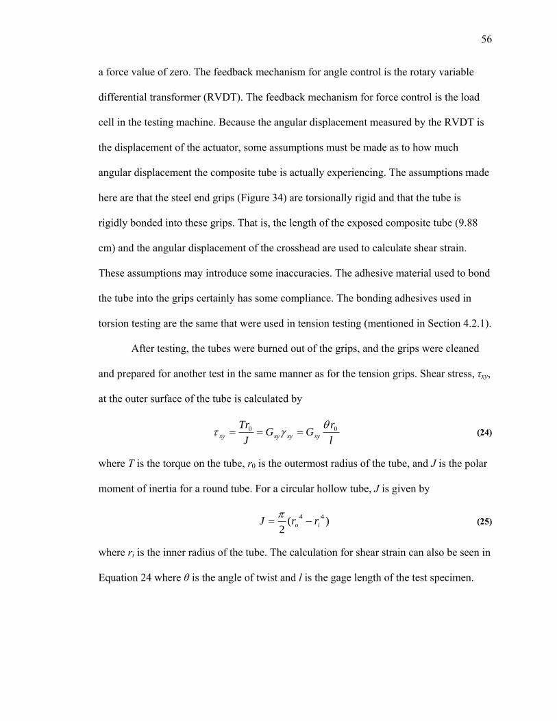
422 Torsion 55
43 Quasi-Static Test Results 57
45 Determination of Ply Elastic Properties 71
46 Summary 78
Chapter 5 Determination of Viscoelastic Lamina Properties 82
51 Material Property Model 82
52 Damping Model 84
53 Experimental Methods for Dynamic Properties 85
54 Master Curves and Model Parameters for Dynamic Properties 92
Chapter 6 Self-heating of Fiber Reinforced Composites 99
61 Modeling 99
611 Closed-Form Analysis 104
vi
612 Finite Element Model 108
6121 The Finite Element ―Building Macro 109
6122 The Finite Element ―Simulation Macro 115
62 Spin Testing 117
621 Experimental Set-Up 117
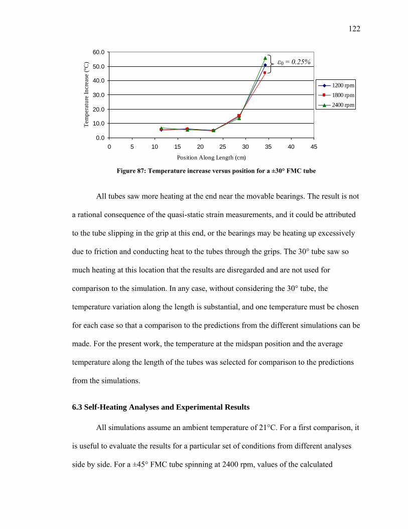
622 Temperature Increase 119
63 Self-Heating Analyses and Experimental Results 122
64 Summary 132
Chapter 7 Conclusions and Recommendations for Future Work 134
References 141
Appendix A ANSYS Macros 147
A1 build1200maclsquo 147
A2 tempincr3maclsquo 158
Appendix B MATLAB Codes 163
B1 main_fraction_2_termmlsquo 163
B2 propsmlsquo 165
Appendix C FEA Mesh Sensitivity Analysis 167
Appendix D Flash Videos 169
D1 Flexible Tube Impactswflsquo 169
D2 Flexible Tube Impact frontswflsquo 170
D3 Rigid Tube Impactswflsquo 171
D4 Flexible 45 Tension Damage strain map frontswflsquo 172
Appendix E Nontechnical Abstract 173
vii
LIST OF FIGURES
Figure 1 Schematic of current driveline design (top) and proposed design (bottom) (Mayrides
2005) 2
Figure 2 Structural (x-y) and principal (1-2) coordinate systems 6
Figure 3 Axial stiffness (Ex) of [plusmnθ]s FMC and RMC laminates 6
Figure 4 Shear stiffness (Gxy) of [plusmnθ]s FMC and RMC laminates 7
Figure 5 Poissonlsquos ratio (νxy) of [plusmnθ]s FMC and RMC laminates 7
Figure 6 Temperature increase for a plusmn60deg T700L100 FMC tube for various speeds and flexural
strain (Shan and Bakis 2009) 11
Figure 7 Rheological model of the fractional derivative standard linear model 15
Figure 8 Schematic of the filament winding machine 24
Figure 9 Filament winder overview (left) and detailed view (right) 27
Figure 10 Glass tow illustrating configuration for hoopwound tubes (left) and
helicalunidirectional tubes (right) 28
Figure 11 Illustration of two cross-hatching diamond patterns around the circumference of a
filament-wound tube 29
Figure 12 Shrink tape application 31
Figure 13 Winding onto a flat plate mandrel to make pre-impregnated sheets of carbon fiber 33
Figure 14 Schematic of the cutting and arranging process of pre-preg in flat specimen mold 34
Figure 15 Closed mold used to make flat plate coupons 35
Figure 16 Composite test specimens left to right 1984 mm tube 991 mm tube 30 mm plate 36
Figure 17 Large Vacuum Gun (LVG) in the NASA GRC ballistic lab 39
Figure 18 Chamber of the LVG 40
Figure 19 FMC tube swelling (left) and contracting (right) after impact plusmn45deg 41
Figure 20 Sequential set of stills FMC tube during impact 25 μs intervals 42
Figure 21 Sequential set of stills RMC tube during impact 25 μs intervals 43
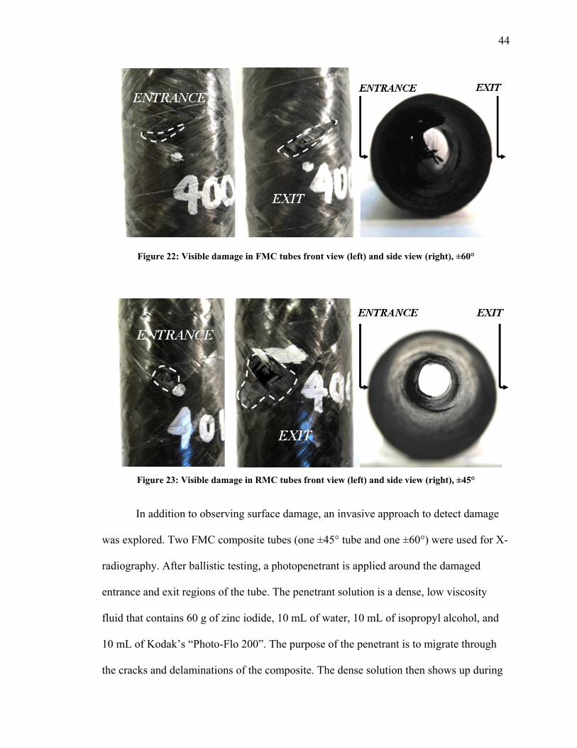
Figure 22 Visible damage in FMC tubes front view (left) and side view (right) plusmn60deg 44
Figure 23 Visible damage in RMC tubes front view (left) and side view (right) plusmn45deg 44
Figure 24 X-radiography image of a flexible plusmn45deg tube after ballistic impact event 45
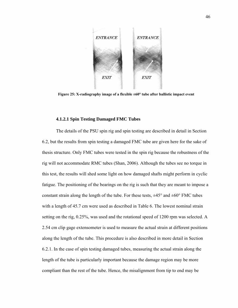
Figure 25 X-radiography image of a flexible plusmn60deg tube after ballistic impact event 46
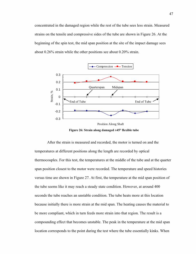
Figure 26 Strain along damaged plusmn45deg flexible tube 47
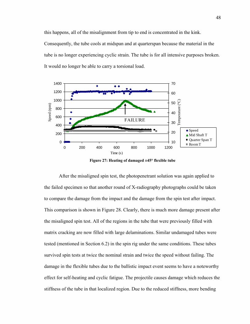
Figure 27 Heating of damaged plusmn45deg flexible tube 48
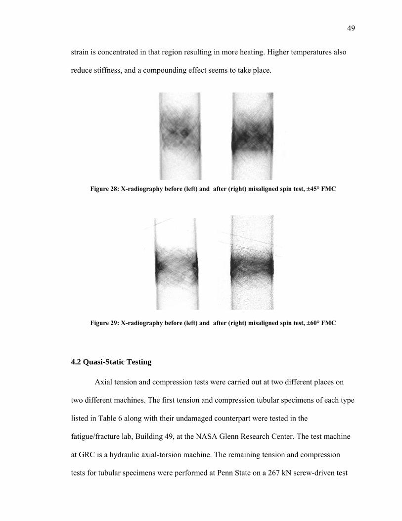
Figure 28 X-radiography before (left) and after (right) misaligned spin test plusmn45deg FMC 49
Figure 29 X-radiography before (left) and after (right) misaligned spin test plusmn60deg FMC 49
viii
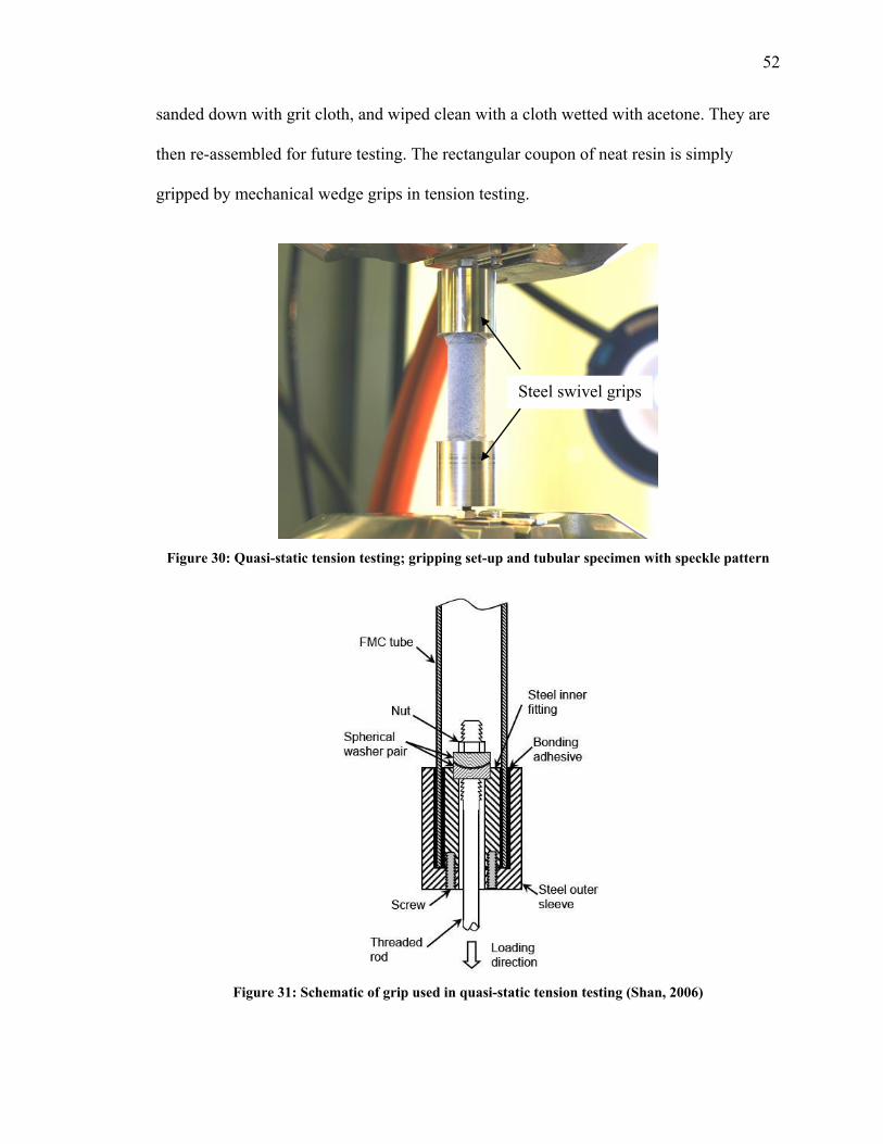
Figure 30 Quasi-static tension testing gripping set-up and tubular specimen with speckle pattern
52
Figure 31 Schematic of grip used in quasi-static tension testing (Shan 2006) 52
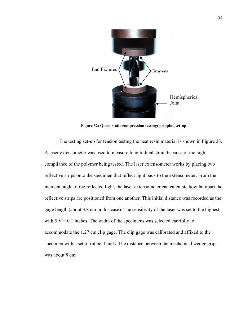
Figure 32 Quasi-static compression testing gripping set-up 54
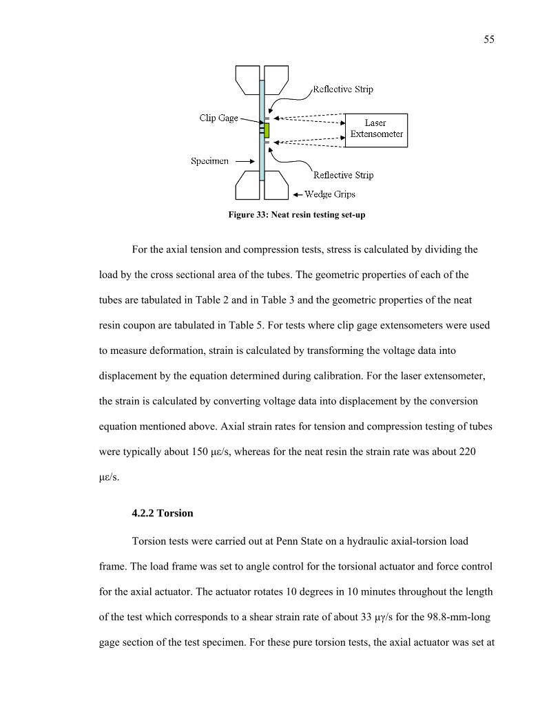
Figure 33 Neat resin testing set-up 55
Figure 34 Steel end grips used in torsion testing 57
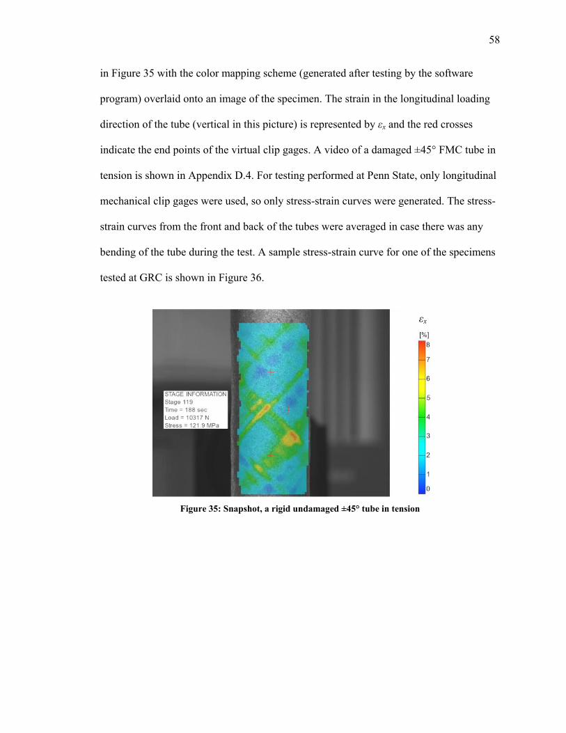
Figure 35 Snapshot a rigid undamaged plusmn45deg tube in tension 58
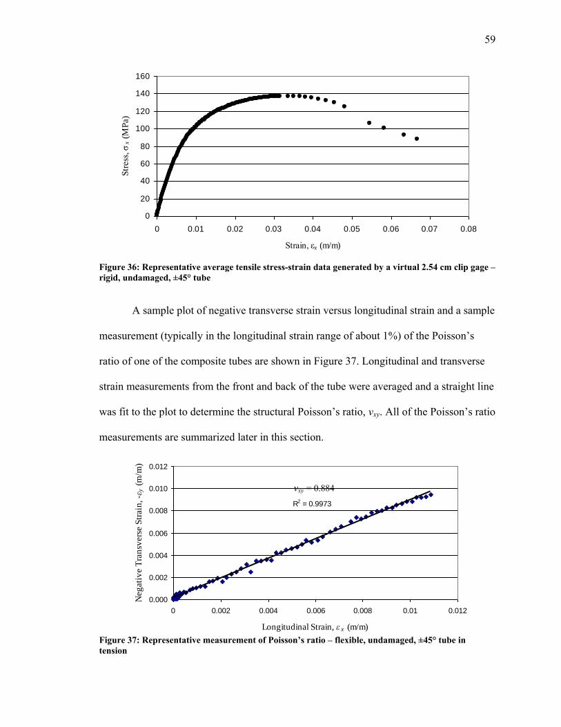
Figure 36 Representative average tensile stress-strain data generated by a virtual 254 cm clip
gage ndash rigid undamaged plusmn45deg tube 59
Figure 37 Representative measurement of Poissonlsquos ratio ndash flexible undamaged plusmn45deg tube in
tension 59
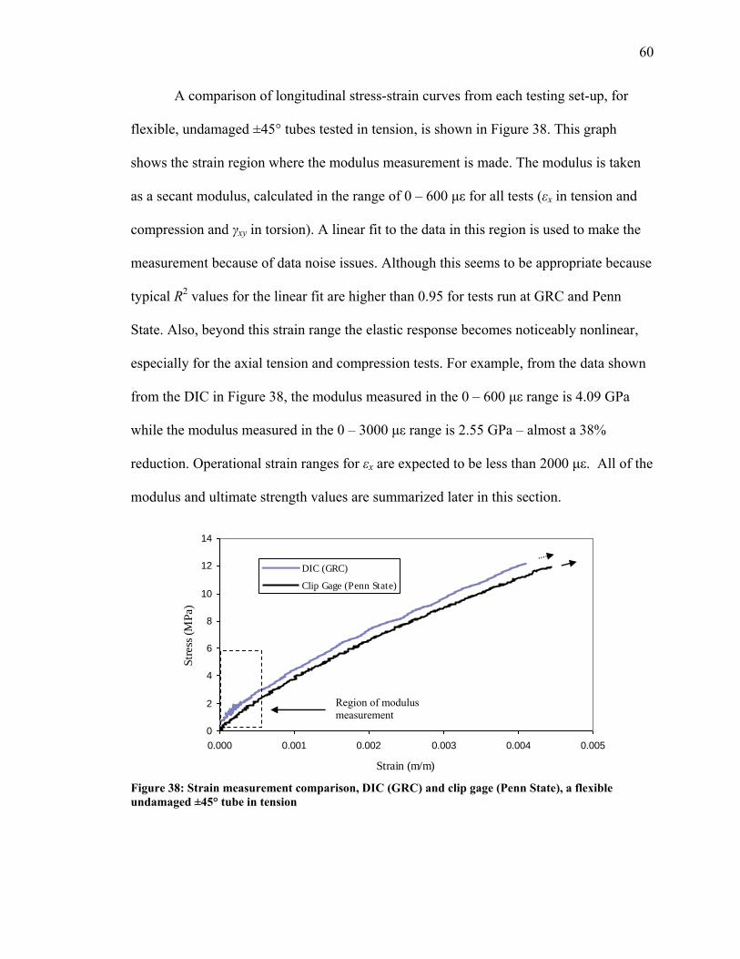
Figure 38 Strain measurement comparison DIC (GRC) and clip gage (Penn State) a flexible
undamaged plusmn45deg tube in tension 60
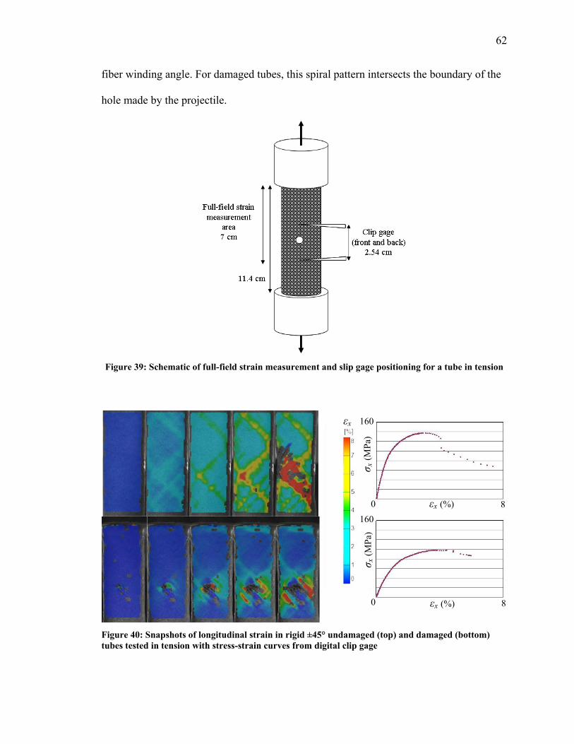
Figure 39 Schematic of full-field strain measurement and slip gage positioning for a tube in
tension 62
Figure 40 Snapshots of longitudinal strain in rigid plusmn45deg undamaged (top) and damaged (bottom)
tubes tested in tension with stress-strain curves from digital clip gage 62
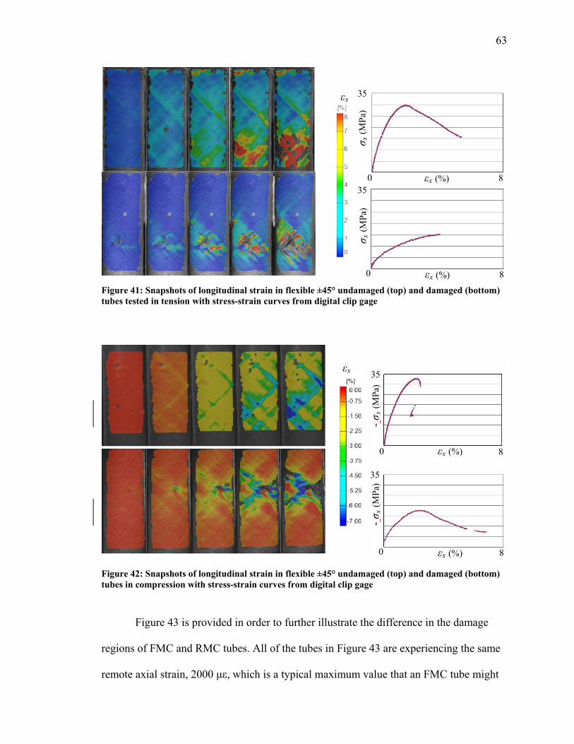
Figure 41 Snapshots of longitudinal strain in flexible plusmn45deg undamaged (top) and damaged
(bottom) tubes tested in tension with stress-strain curves from digital clip gage 63
Figure 42 Snapshots of longitudinal strain in flexible plusmn45deg undamaged (top) and damaged
(bottom) tubes in compression with stress-strain curves from digital clip gage 63
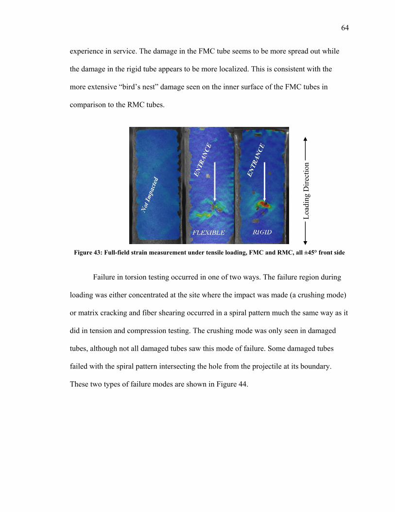
Figure 43 Full-field strain measurement under tensile loading FMC and RMC all plusmn45deg front
side 64
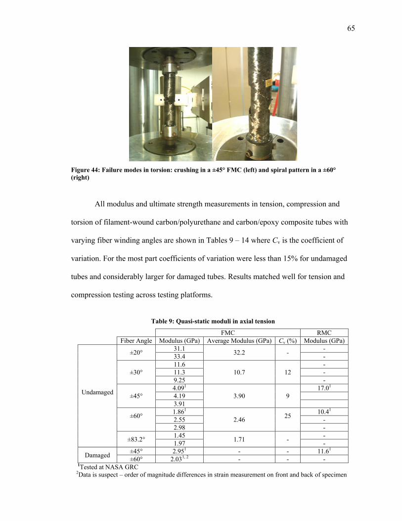
Figure 44 Failure modes in torsion crushing in a plusmn45deg FMC (left) and spiral pattern in a plusmn60deg
(right) 65
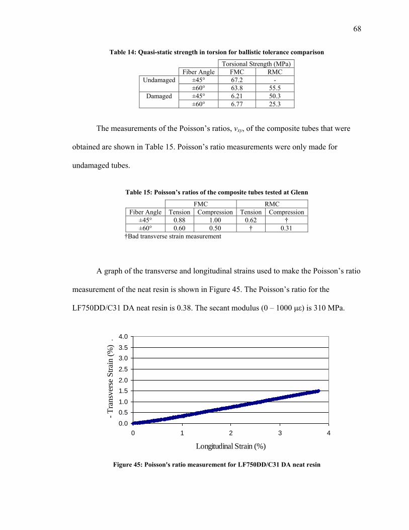
Figure 45 Poissons ratio measurement for LF750DDC31 DA neat resin 68
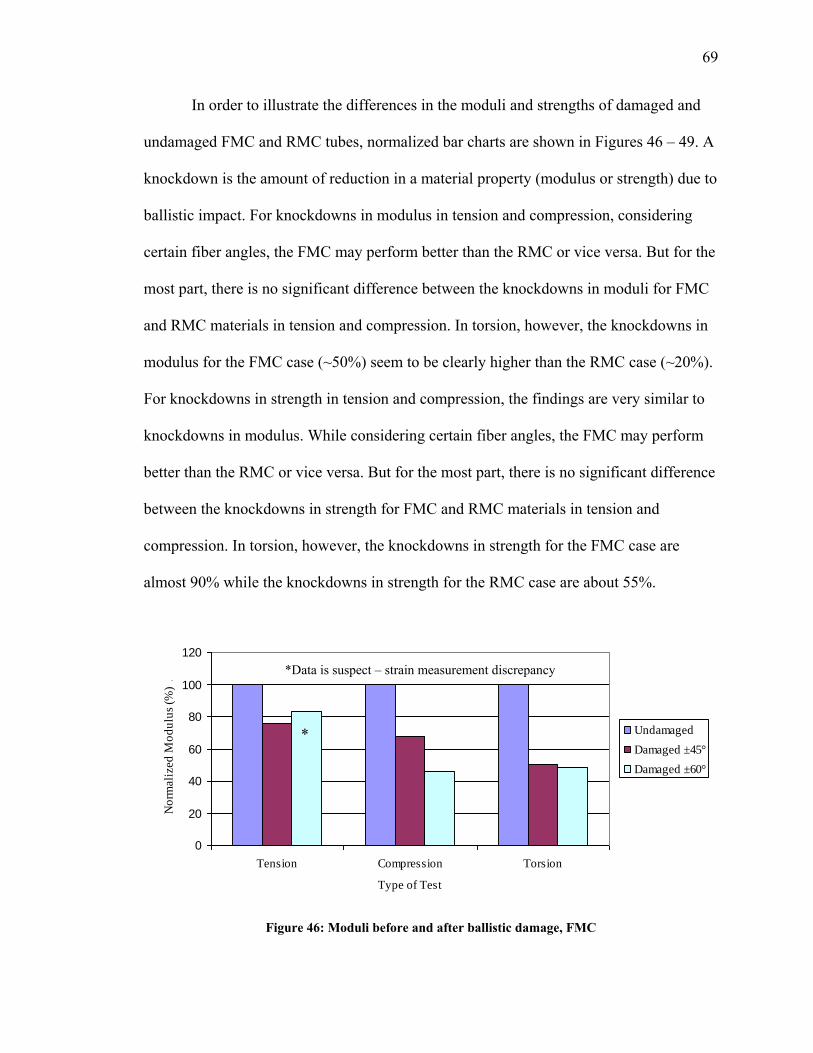
Figure 46 Moduli before and after ballistic damage FMC 69
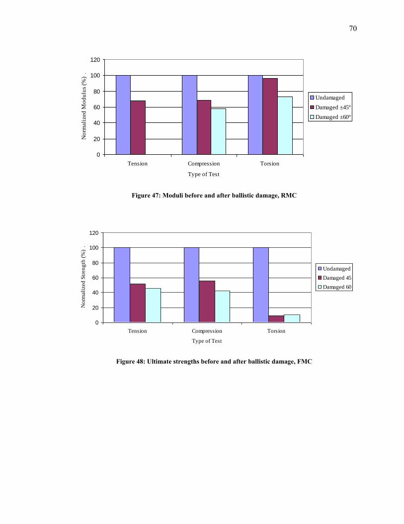
Figure 47 Moduli before and after ballistic damage RMC 70
Figure 48 Ultimate strengths before and after ballistic damage FMC 70
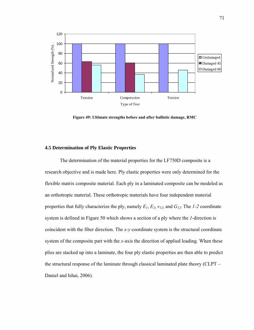
Figure 49 Ultimate strengths before and after ballistic damage RMC 71
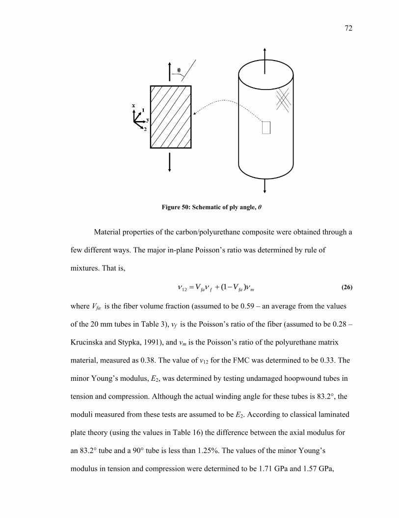
Figure 50 Schematic of ply angle θ 72
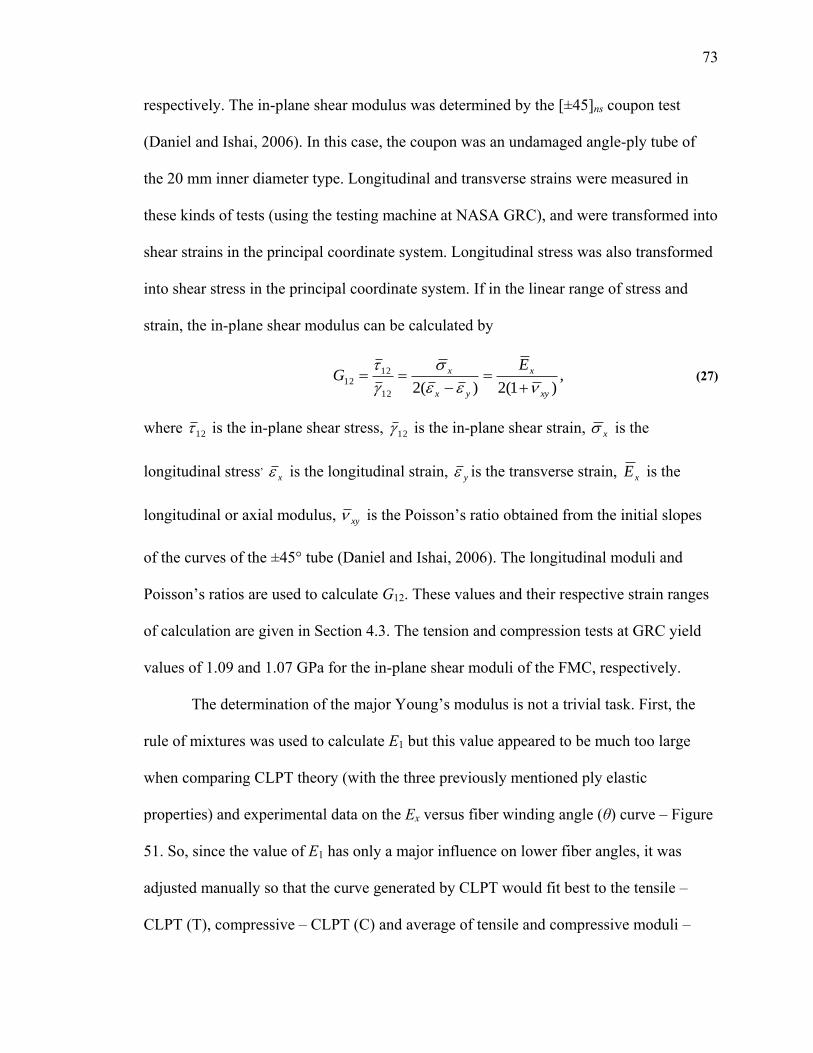
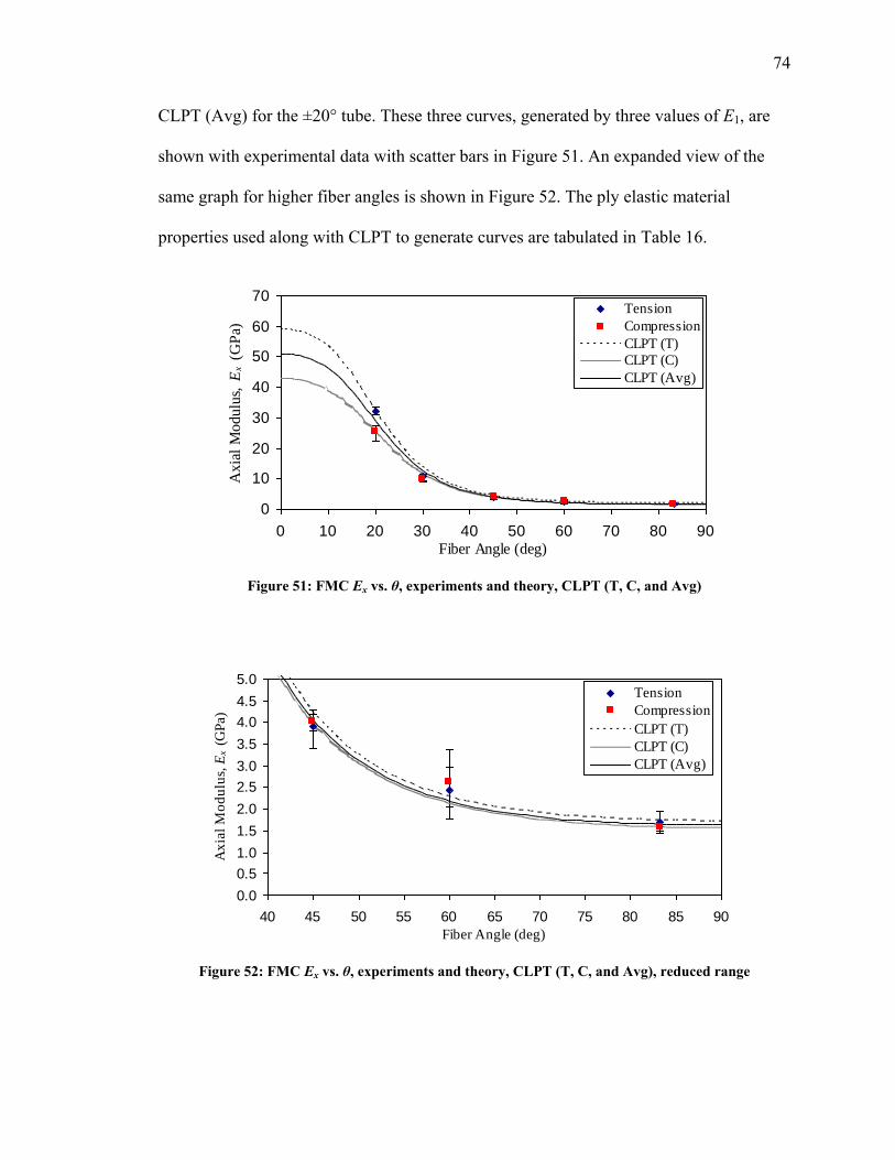
Figure 51 FMC Ex vs θ experiments and theory CLPT (T C and Avg) 74
Figure 52 FMC Ex vs θ experiments and theory CLPT (T C and Avg) reduced range 74
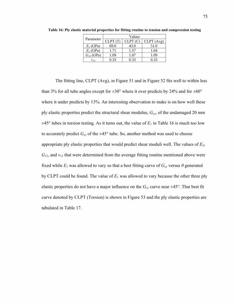
Figure 53 Gxy vs θ experiments and theory CLPT (Torsion) 76
ix
Figure 54 Ex vs θ experiments and theory CLPT (Avg and Torsion) 77
Figure 55 Ex vs θ experiments and theory CLPT (Avg and Torsion) reduced range 77
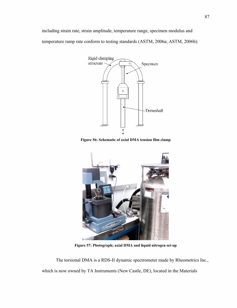
Figure 56 Schematic of axial DMA tension film clamp 87
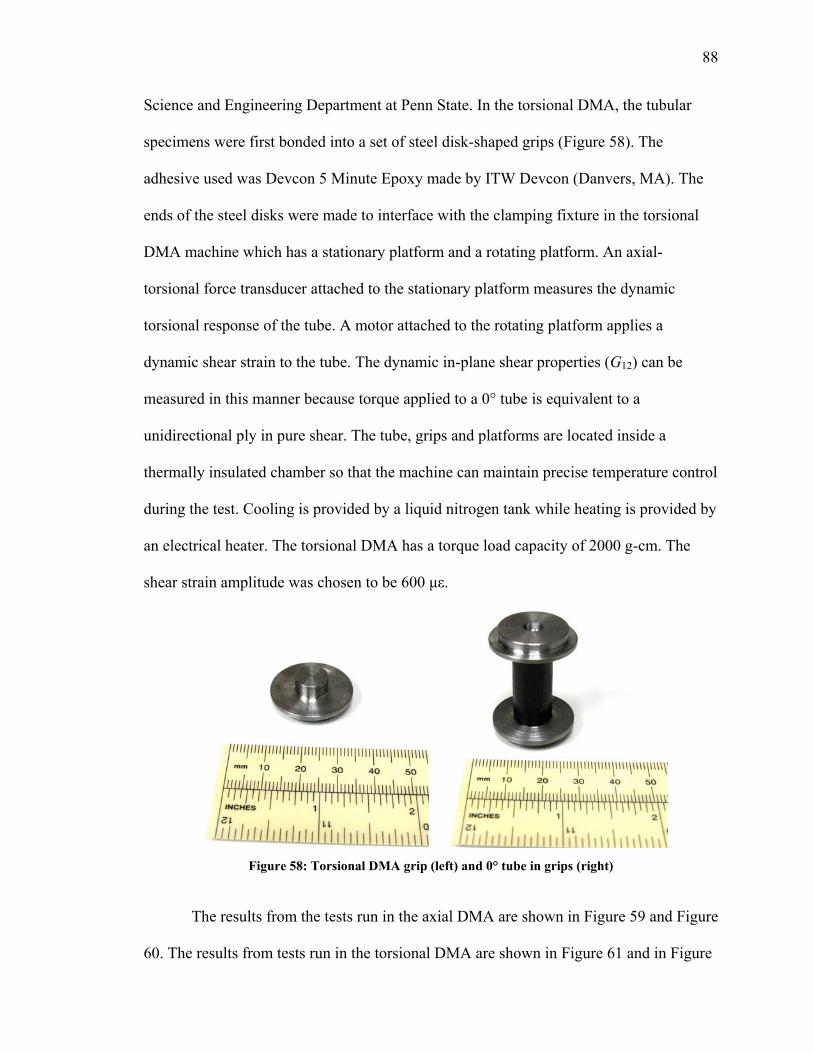
Figure 57 Photograph axial DMA and liquid nitrogen set-up 87
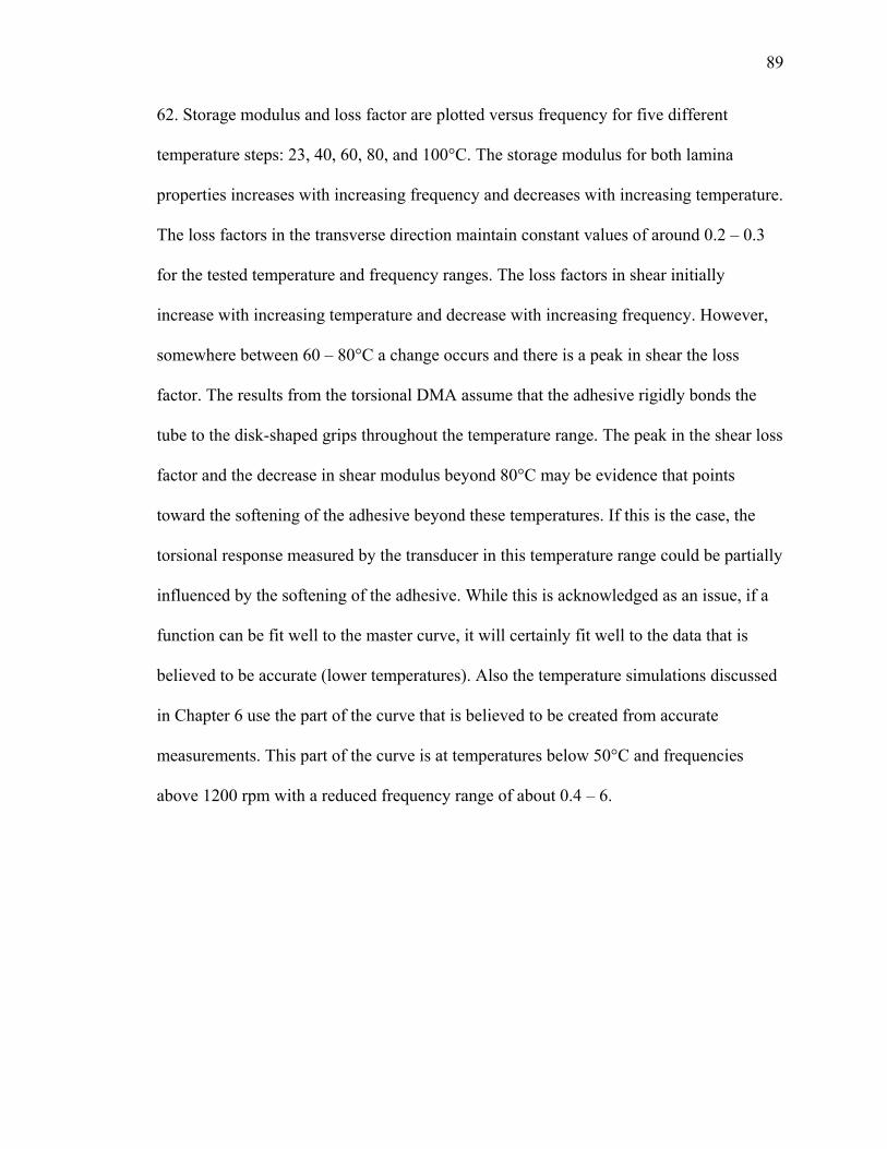
Figure 58 Torsional DMA grip (left) and 0deg tube in grips (right) 88
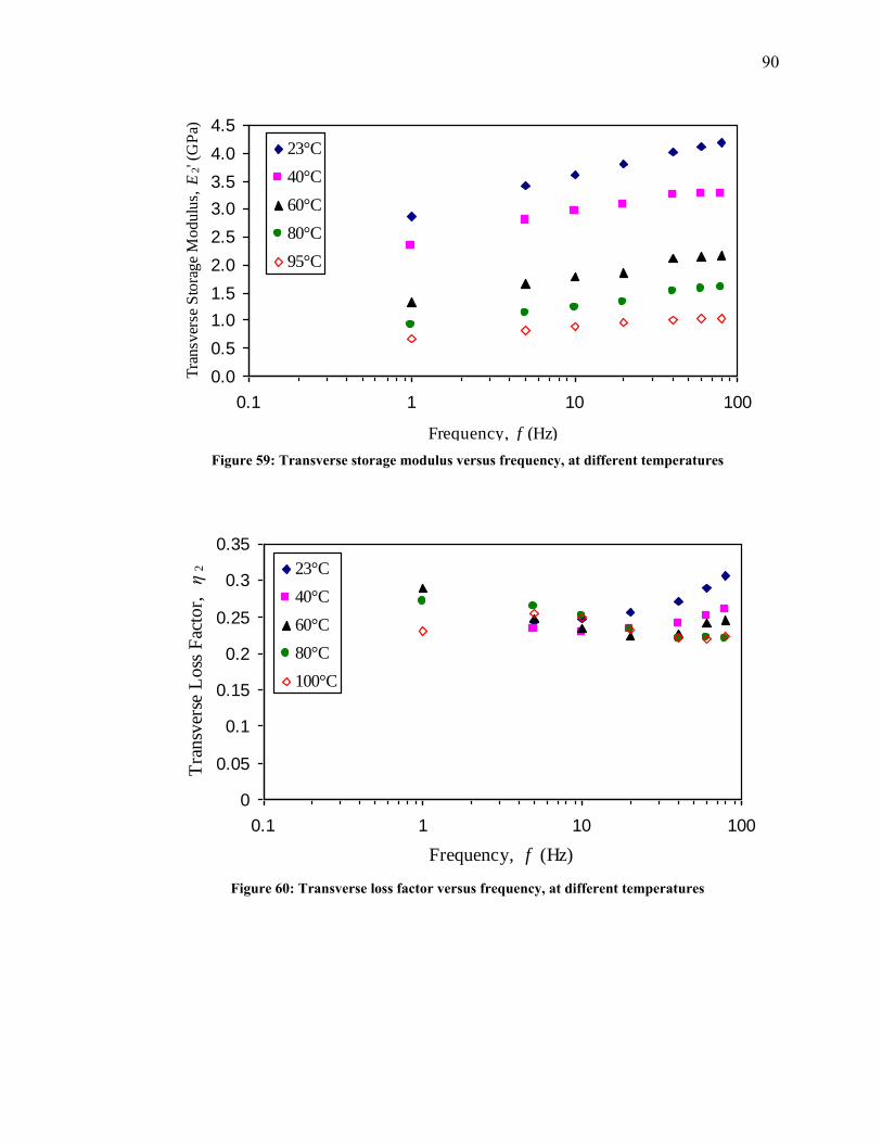
Figure 59 Transverse storage modulus versus frequency at different temperatures 90
Figure 60 Transverse loss factor versus frequency at different temperatures 90
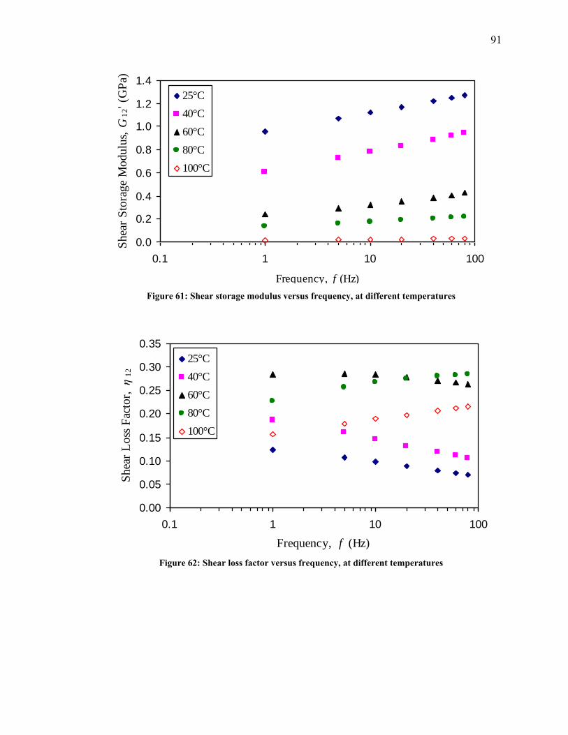
Figure 61 Shear storage modulus versus frequency at different temperatures 91
Figure 62 Shear loss factor versus frequency at different temperatures 91
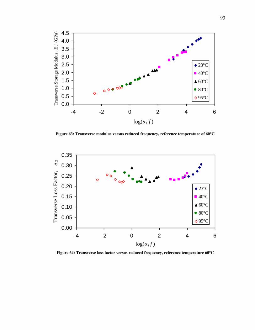
Figure 63 Transverse modulus versus reduced frequency reference temperature of 60degC 93
Figure 64 Transverse loss factor versus reduced frequency reference temperature 60degC 93
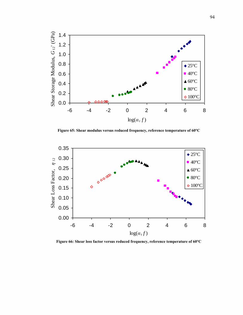
Figure 65 Shear modulus versus reduced frequency reference temperature of 60degC 94
Figure 66 Shear loss factor versus reduced frequency reference temperature of 60degC 94
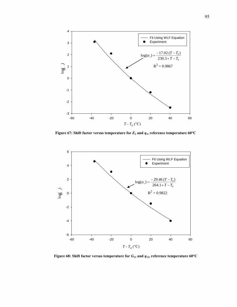
Figure 67 Shift factor versus temperature for E2 and η2 reference temperature 60degC 95
Figure 68 Shift factor versus temperature for G12 and η12 reference temperature 60degC 95
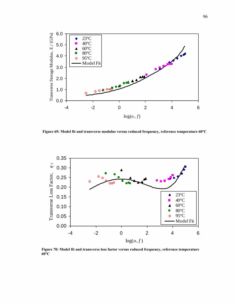
Figure 69 Model fit and transverse modulus versus reduced frequency reference temperature
60degC 96
Figure 70 Model fit and transverse loss factor versus reduced frequency reference temperature
60degC 96
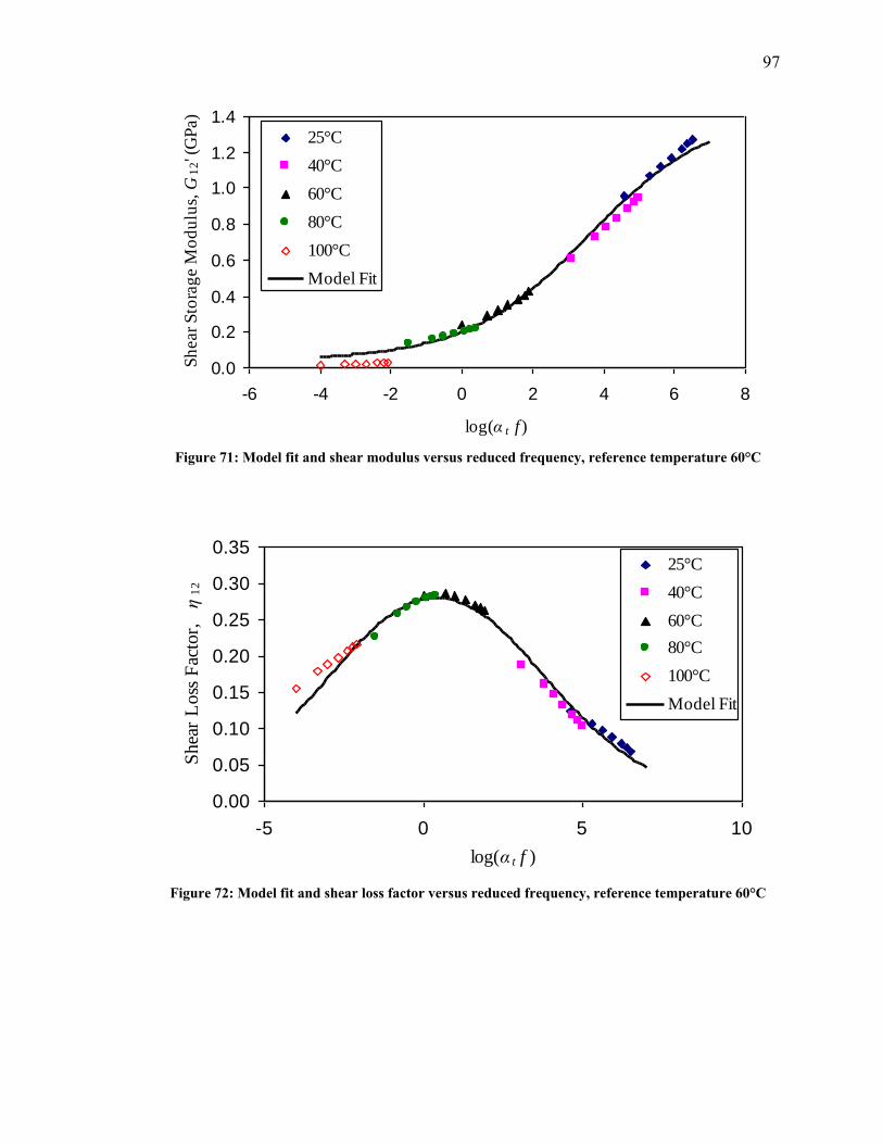
Figure 71 Model fit and shear modulus versus reduced frequency reference temperature 60degC 97
Figure 72 Model fit and shear loss factor versus reduced frequency reference temperature 60degC
97
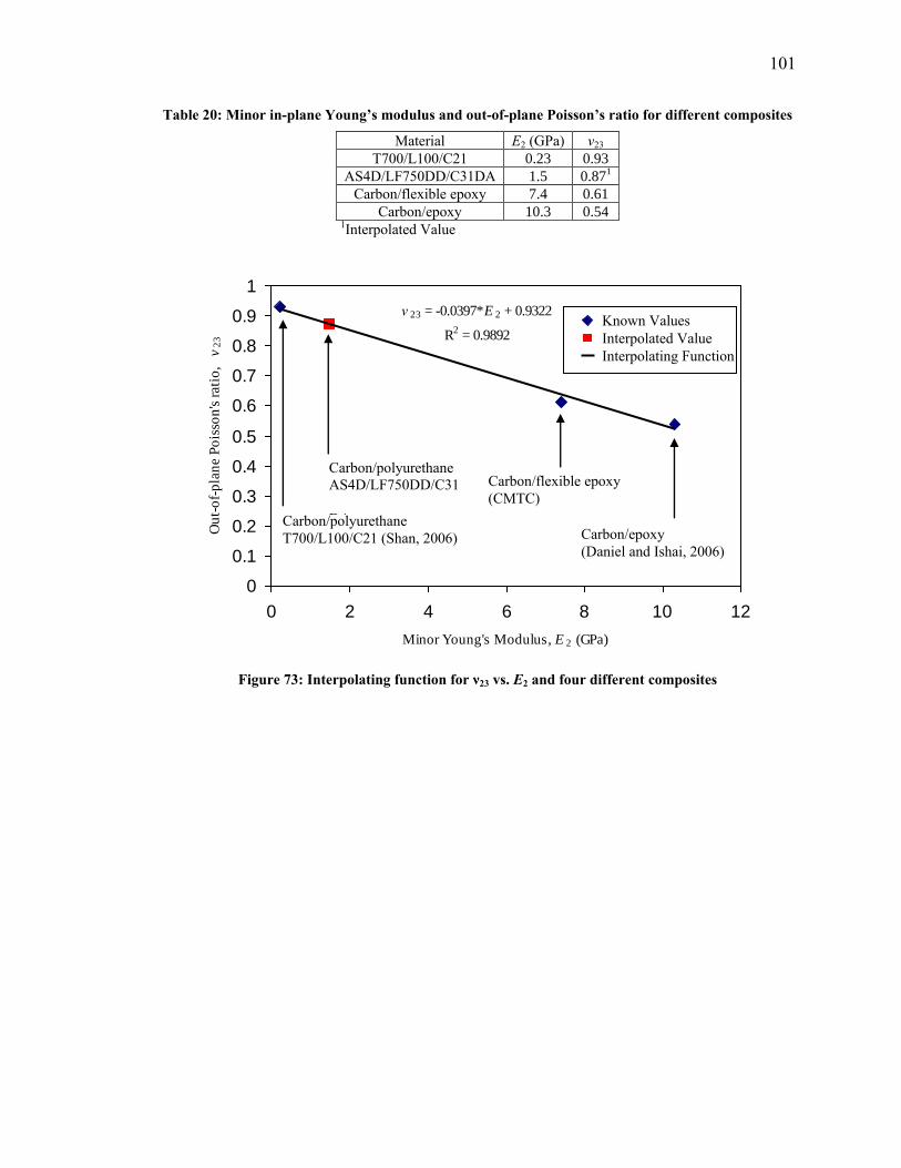
Figure 73 Interpolating function for ν23 vs E2 and four different composites 101
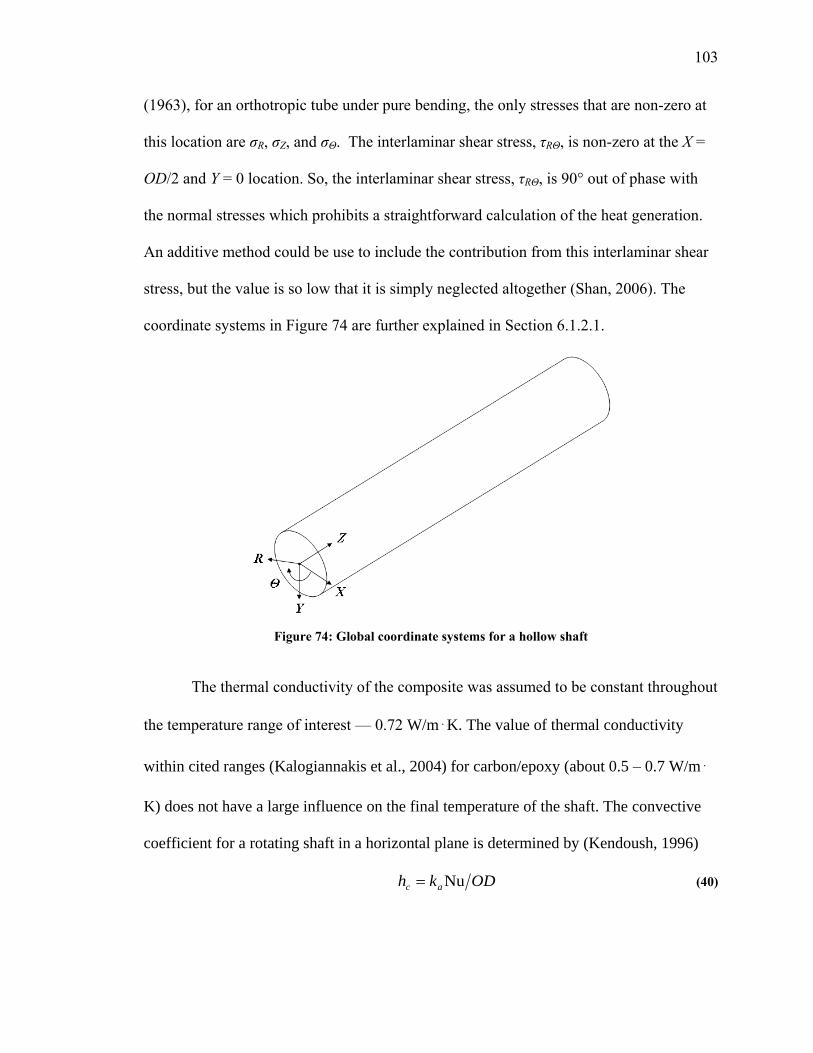
Figure 74 Global coordinate systems for a hollow shaft 103
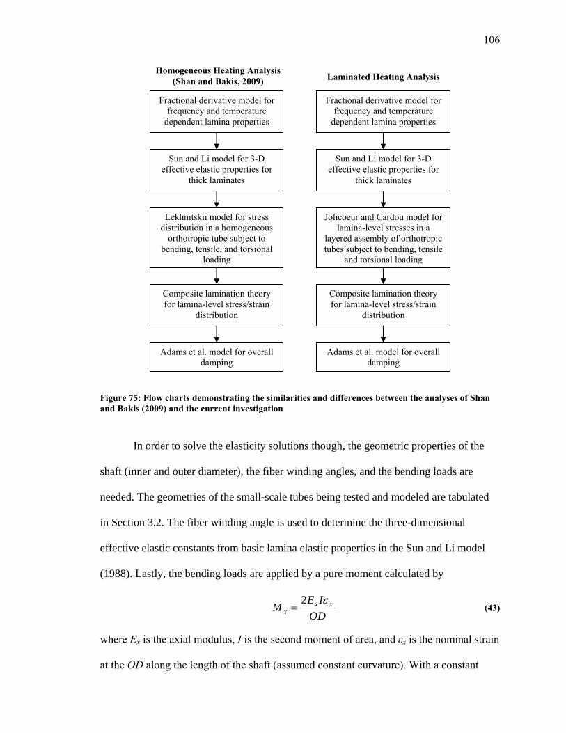
Figure 75 Flow charts demonstrating the similarities and differences between the analyses of
Shan and Bakis (2009) and the current investigation 106
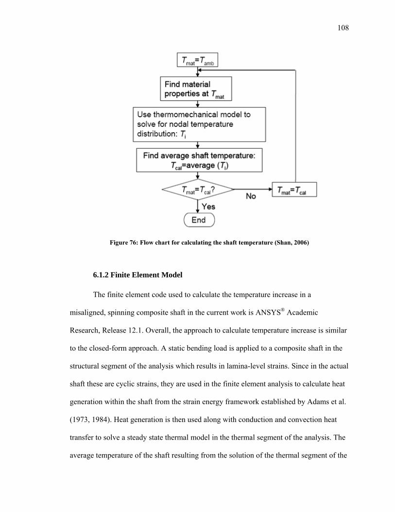
Figure 76 Flow chart for calculating the shaft temperature (Shan 2006) 108
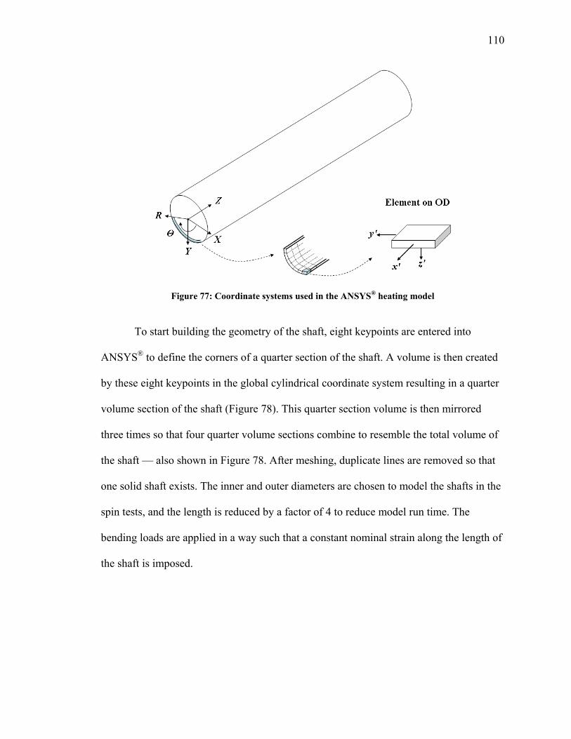
Figure 77 Coordinate systems used in the ANSYSreg heating model 110
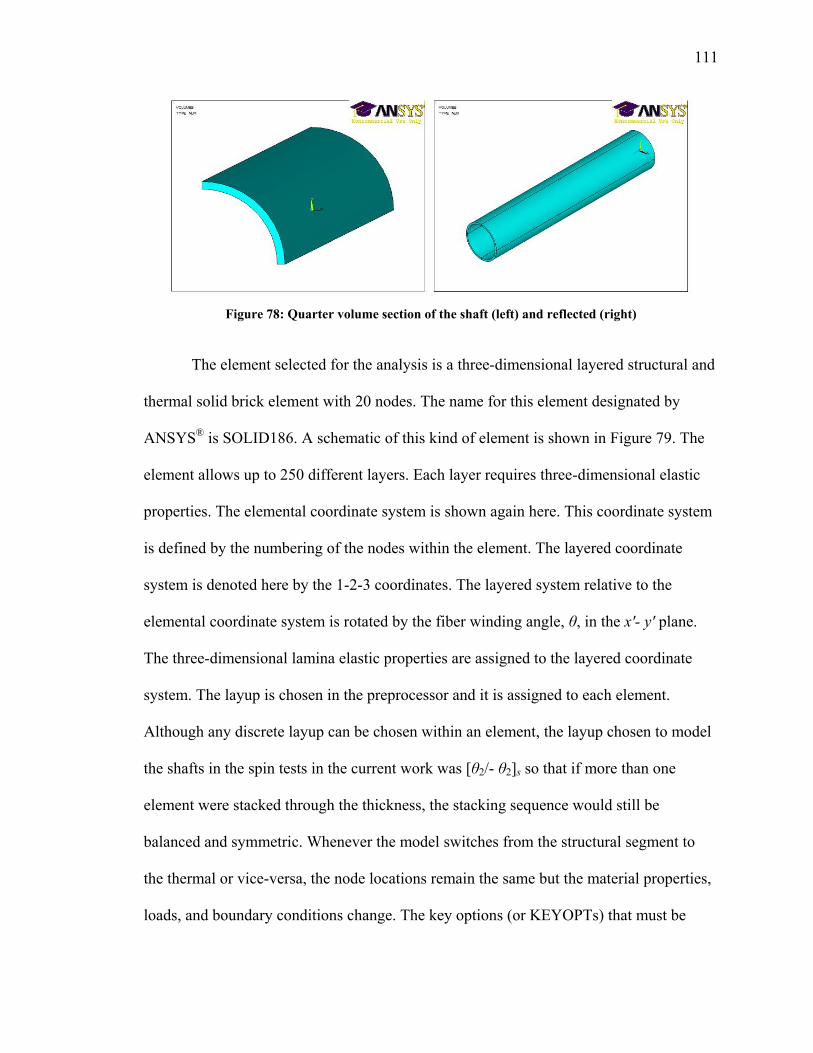
Figure 78 Quarter volume section of the shaft (left) and reflected (right) 111
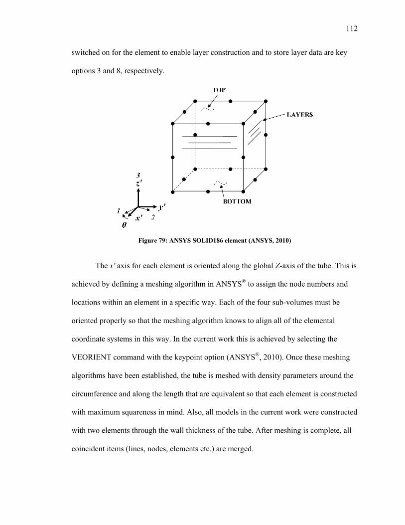
Figure 79 ANSYS SOLID186 element (ANSYS 2010) 112
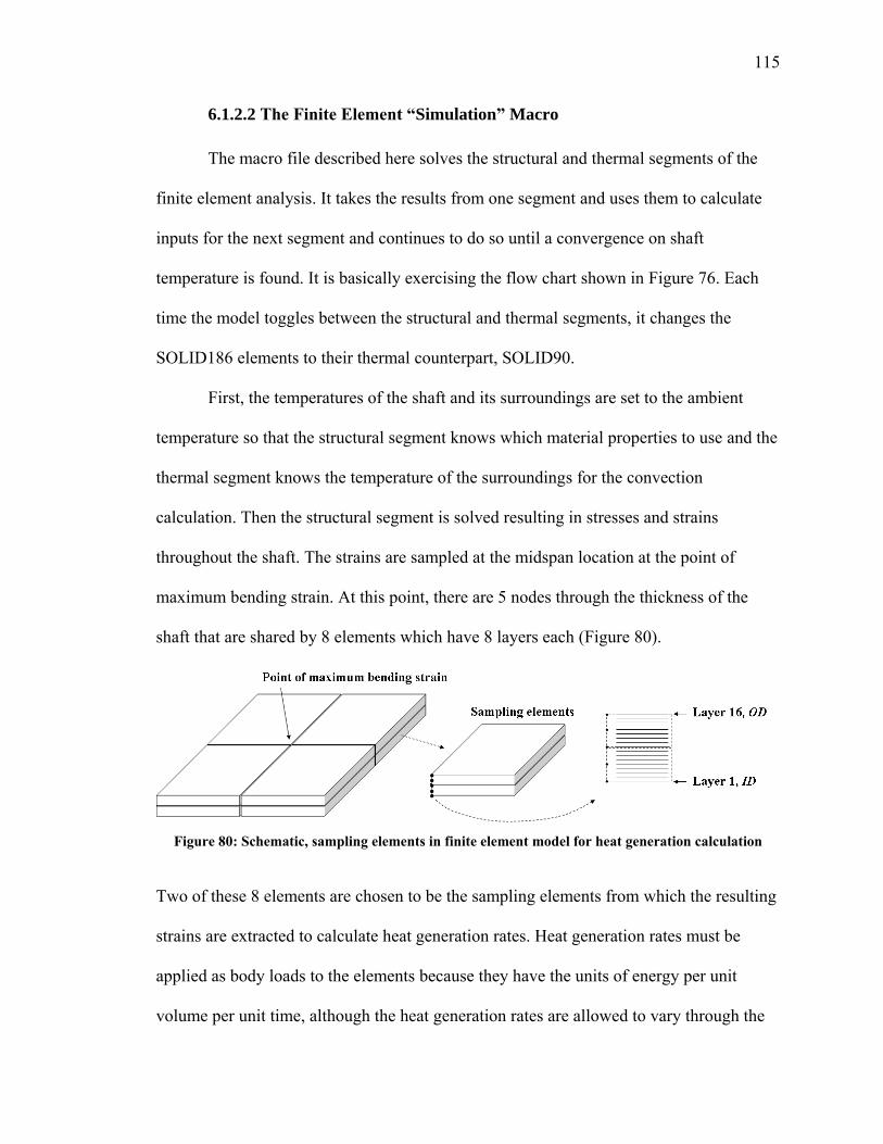
Figure 80 Schematic sampling elements in finite element model for heat generation calculation
115
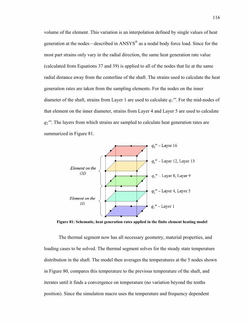
Figure 81 Schematic heat generation rates applied in the finite element heating model 116
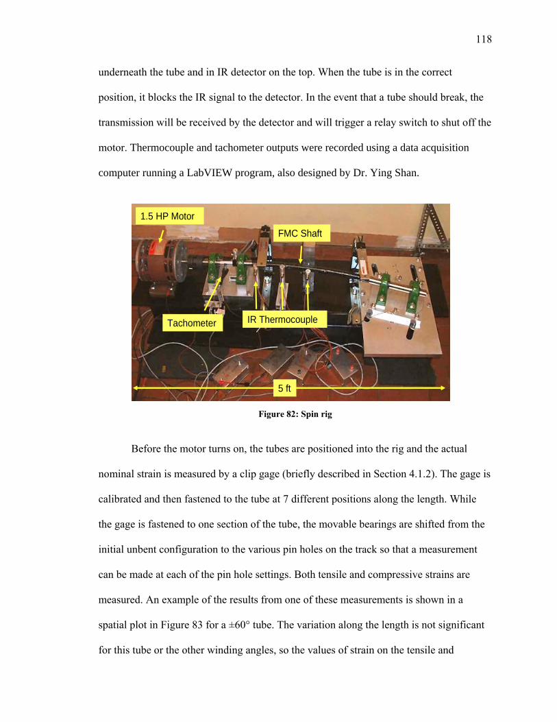
Figure 82 Spin rig 118
x
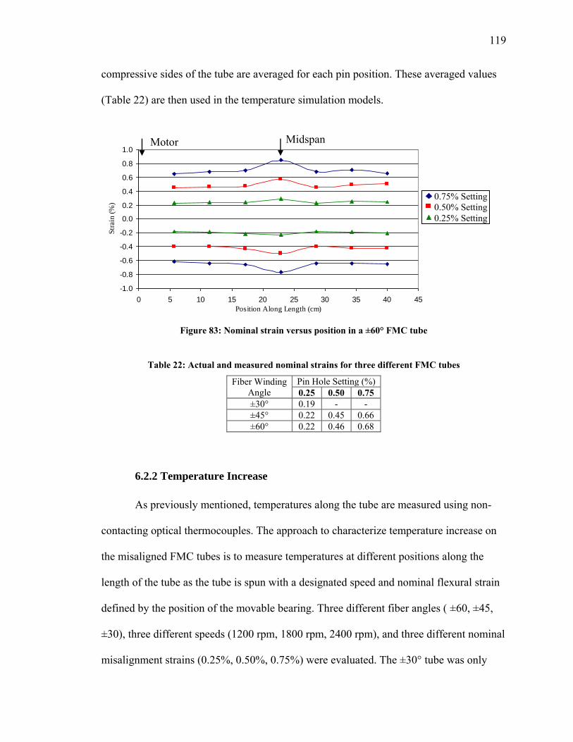
Figure 83 Nominal strain versus position in a plusmn60deg FMC tube 119
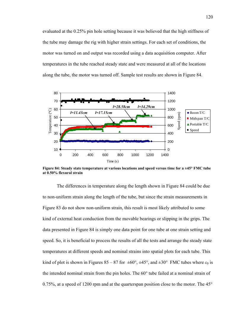
Figure 84 Steady state temperature at various locations and speed versus time for a plusmn45deg FMC
tube at 050 flexural strain 120
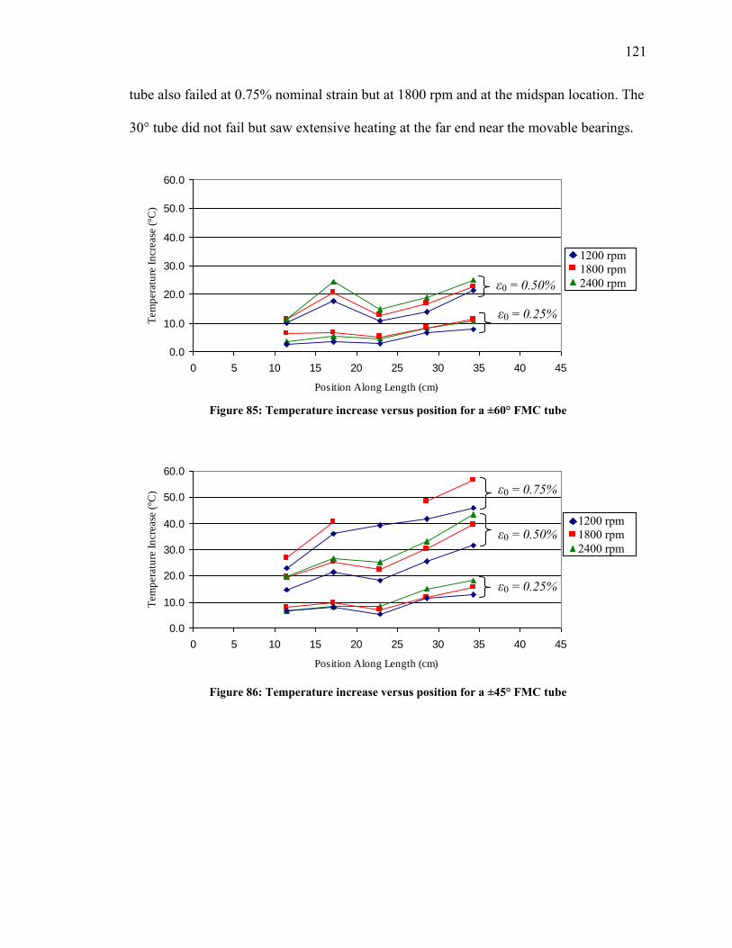
Figure 85 Temperature increase versus position for a plusmn60deg FMC tube 121
Figure 86 Temperature increase versus position for a plusmn45deg FMC tube 121
Figure 87 Temperature increase versus position for a plusmn30deg FMC tube 122
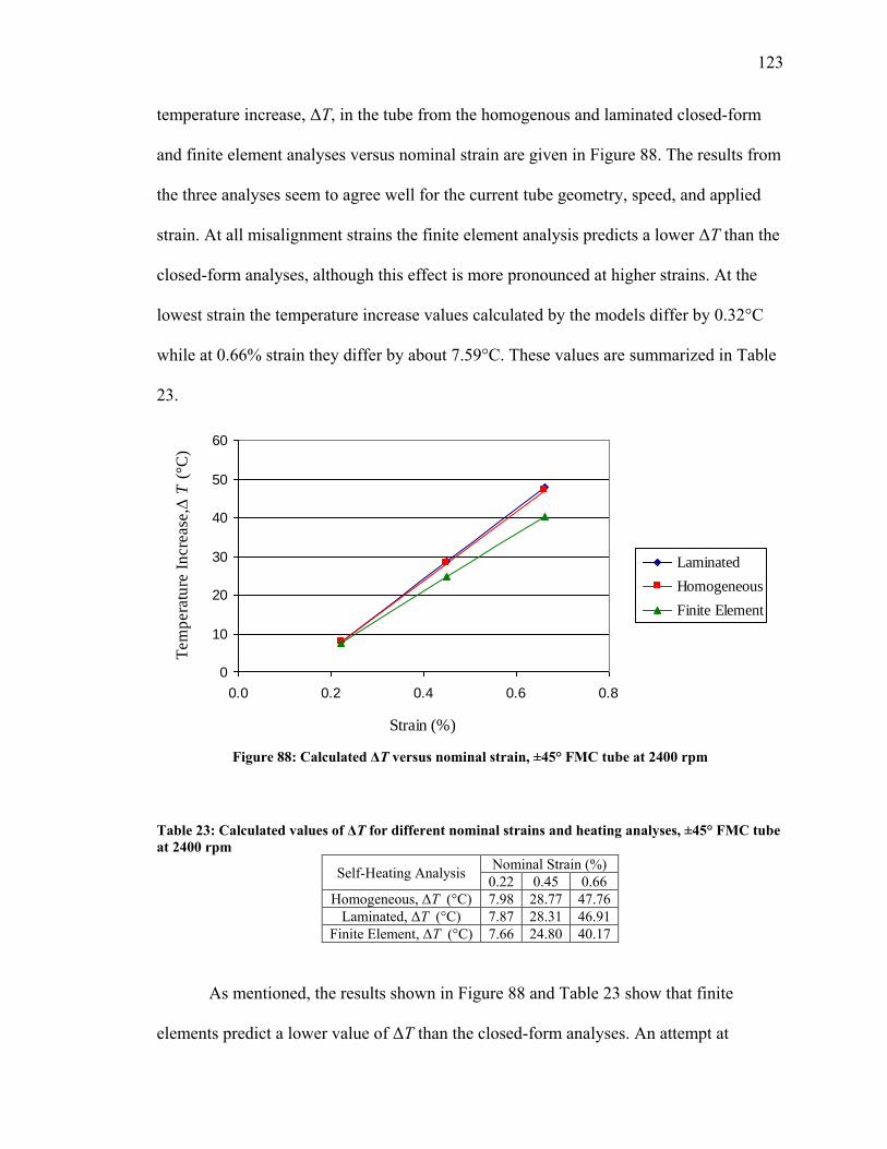
Figure 88 Calculated ΔT versus nominal strain plusmn45deg FMC tube at 2400 rpm 123
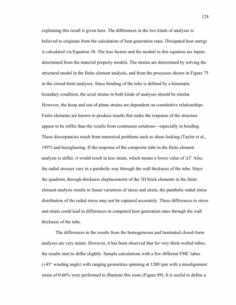
Figure 89 Calculations of ΔT by the closed-form heating analyses for different tube geometries
plusmn45deg FMC at 1200 rpm and 066 misalignment strain 125
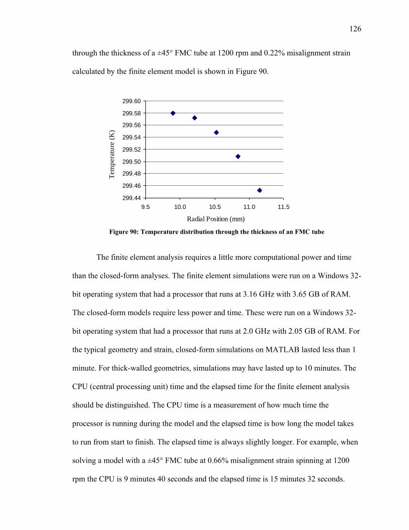
Figure 90 Temperature distribution through the thickness of an FMC tube 126
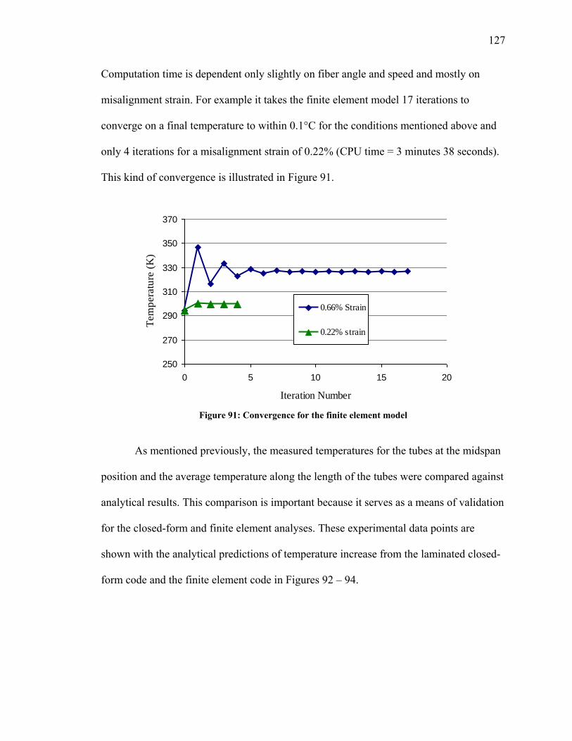
Figure 91 Convergence for the finite element model 127
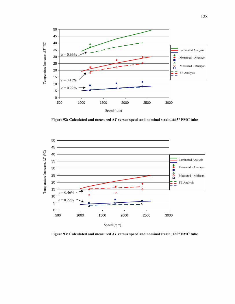
Figure 92 Calculated and measured ΔT versus speed and nominal strain plusmn45deg FMC tube 128
Figure 93 Calculated and measured ΔT versus speed and nominal strain plusmn60deg FMC tube 128
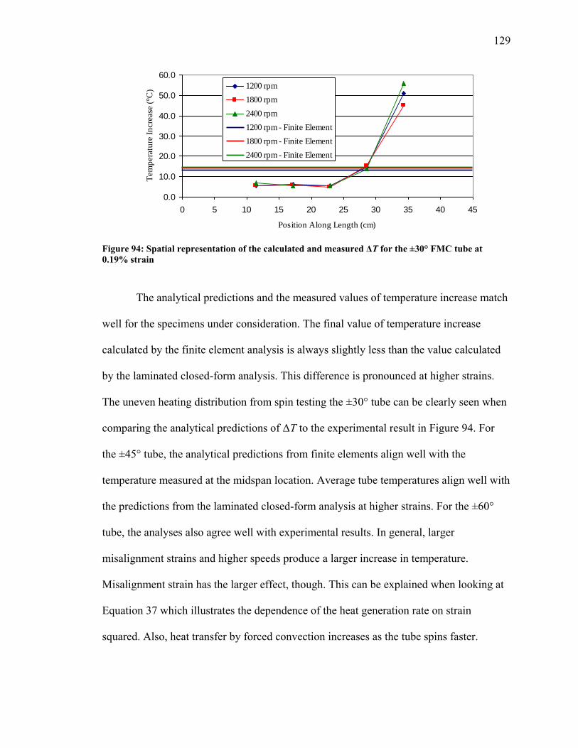
Figure 94 Spatial representation of the calculated and measured ΔT for the plusmn30deg FMC tube at
019 strain 129
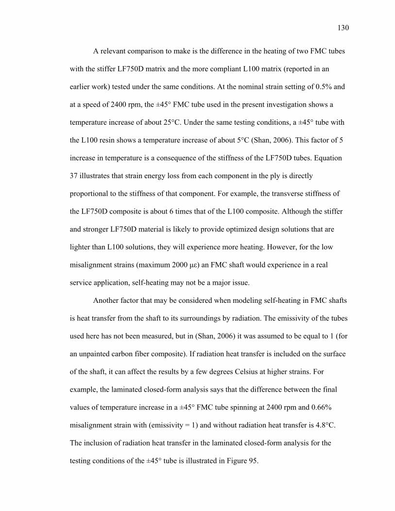
Figure 95 Calculated ΔT with and without radiation versus speed and nominal strain plusmn45deg FMC
tube 131
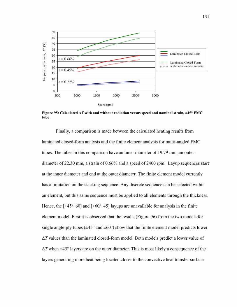
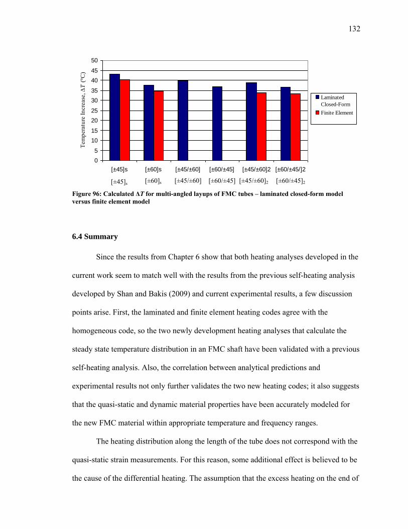
Figure 96 Calculated ΔT for multi-angled layups of FMC tubes ndash laminated closed-form model
versus finite element model 132
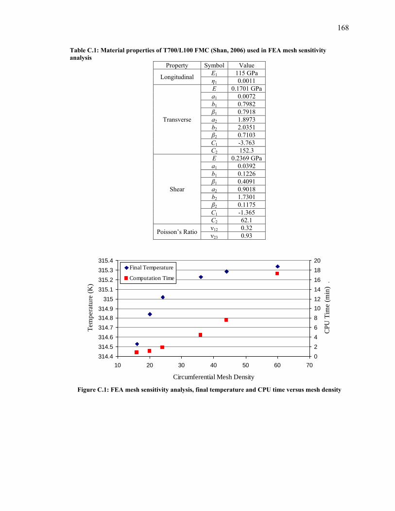
Figure C1 FEA mesh sensitivity analysis final temperature and CPU time versus mesh density
helliphelliphelliphelliphelliphelliphelliphelliphelliphelliphelliphelliphelliphelliphelliphelliphelliphelliphelliphelliphelliphelliphelliphelliphelliphelliphelliphelliphelliphelliphelliphelliphelliphelliphelliphelliphellip168
xi
LIST OF TABLES
Table 1 Quasi-static ply elastic properties for an FMC and RMC 6
Table 2 Geometric properties and fiber volume fractions of the carbonepoxy tubes 30
Table 3 Geometric properties and fiber volume fractions of the carbonpolyurethane tubes 31
Table 4 Geometric properties of the 90deg flat plate coupons used in dynamic testing 35
Table 5 Geometric properties of neat resin testing coupon 35
Table 6 Quantity of each specimen type used in ballistic testing 38
Table 7 Pre and post impact velocities energies 42
Table 8 Test matrix for undamaged composite tubes 57
Table 9 Quasi-static moduli in axial tension 65
Table 10 Quasi-static moduli in axial compression 66
Table 11 Quasi-static moduli in torsion 66
Table 12 Quasi-static ultimate strength in axial tension 67
Table 13 Quasi-static ultimate strength in axial compression 67
Table 14 Quasi-static strength in torsion for ballistic tolerance comparison 68
Table 15 Poissonlsquos ratios of the composite tubes tested at Glenn 68
Table 16 Ply elastic material properties for fitting routine to tension and compression testing 75
Table 17 Ply elastic material properties for fitting routine to torsion testing 76
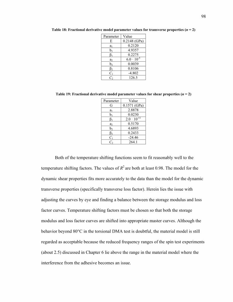
Table 18 Fractional derivative model parameter values for transverse properties (n = 2) 98
Table 19 Fractional derivative model parameter values for shear properties (n = 2) 98
Table 20 Minor in-plane Younglsquos modulus and out-of-plane Poissonlsquos ratio for different
composites 101
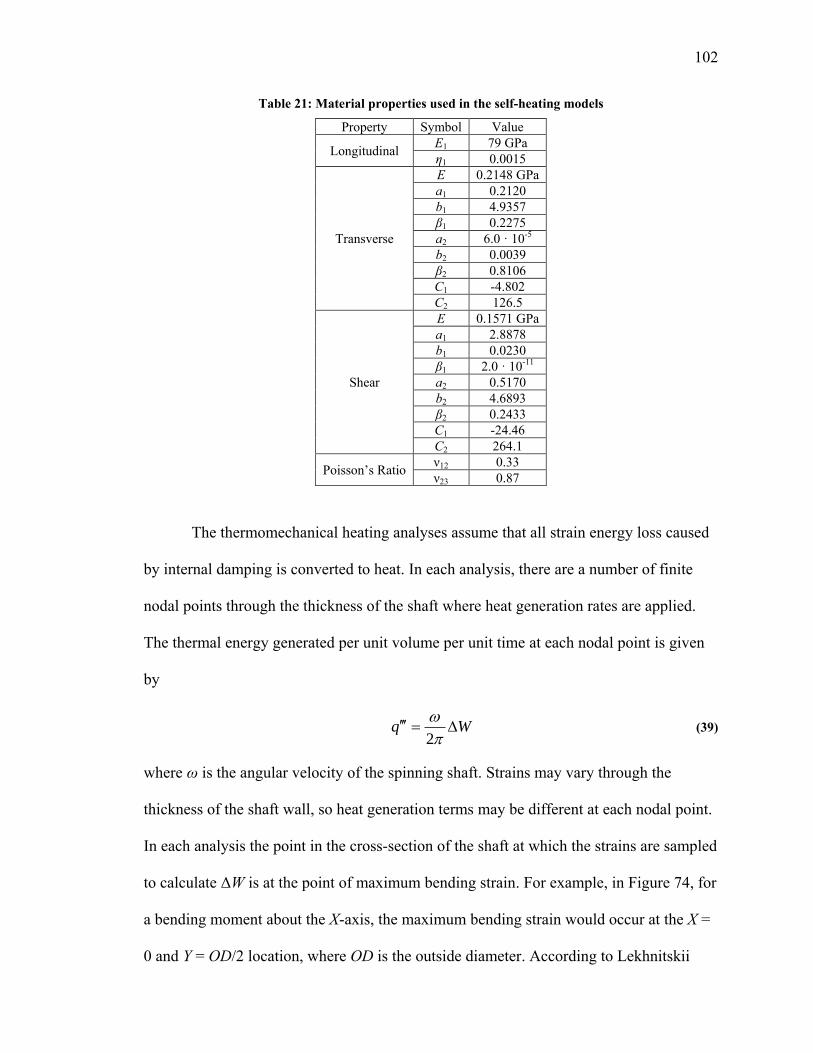
Table 21 Material properties used in the self-heating models 102
Table 22 Actual and measured nominal strains for three different FMC tubes 119
Table 23 Calculated values of ΔT for different nominal strains and heating analyses plusmn45deg FMC
tube at 2400 rpm 123
Table C1 Material properties of T700L100 FMC (Shan 2006) used in FEA mesh sensitivity
analysishelliphelliphelliphelliphelliphelliphelliphelliphelliphelliphelliphelliphelliphelliphelliphelliphelliphelliphelliphelliphelliphelliphelliphelliphelliphelliphelliphelliphelliphelliphelliphelliphelliphellip168
xii
ACKNOWLEDGEMENTS
First I would like to thank my advisor Dr Charles Bakis for always finding time
to provide thoughtful guidance for me during the course of my studies at Penn State I
would like to acknowledge Dr Edward Smith Dr Gary Roberts Mr Monte McGlaun
and Mr Russell Mueller for their valuable technical discussions and support I would like
to thank Dr Clifford Lissenden Dr Bo Kasal Dr Ralph Colby and Dr Nicole Brown
for the use of their laboratory equipment Also Dr Mike Pereira Mr Justin Bail Mr
Chuck Ruggeri Mr Simon Miller Mr U Hyeok Choi Mr Todd Henry Mr Steve Smith
and Mr Robert Blass provided a great deal of help to me in the laboratories that were
used to conduct this research Harish Chandra and Ian Laskowitz from the Chemtura
Corporation were very helpful in providing some materials for this research some on a
free sample basis
This research was funded in part by the Center for Rotorcraft Innovation (CRI)
and the National Rotorcraft Technology Center (NRTC) US Army Aviation and Missile
Research Development and Engineering Center (AMRDEC) under Technology
Investment Agreement W911W6-05-2-0003 entitled National Rotorcraft Technology
Center Research Program The author would like to acknowledge that this research and
development was accomplished with the support and guidance of the NRTC and CRI
Additional sources of funding include Bell Helicopter Textron through the Bell
Helicopter Fellowship the American Helicopter Society through their Vertical Flight
Foundation scholarship and the American Helicopter Society in conjunction with NASA
through their Summer Internship Award
xiii
The views and conclusions contained in this document are those of the author and
should not be interpreted as representing the official policies either expressed or implied
of the AMRDEC or the US Government The US Government is authorized to
reproduce and distribute reprints for Government purposes notwithstanding any copyright
notation thereon
1
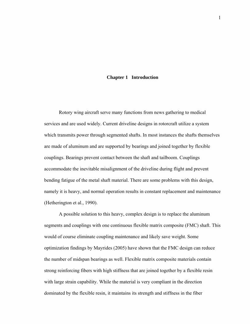
Chapter 1 Introduction
Rotory wing aircraft serve many functions from news gathering to medical
services and are used widely Current driveline designs in rotorcraft utilize a system
which transmits power through segmented shafts In most instances the shafts themselves
are made of aluminum and are supported by bearings and joined together by flexible
couplings Bearings prevent contact between the shaft and tailboom Couplings
accommodate the inevitable misalignment of the driveline during flight and prevent
bending fatigue of the metal shaft material There are some problems with this design
namely it is heavy and normal operation results in constant replacement and maintenance
(Hetherington et al 1990)
A possible solution to this heavy complex design is to replace the aluminum
segments and couplings with one continuous flexible matrix composite (FMC) shaft This
would of course eliminate coupling maintenance and likely save weight Some
optimization findings by Mayrides (2005) have shown that the FMC design can reduce
the number of midspan bearings as well Flexible matrix composite materials contain
strong reinforcing fibers with high stiffness that are joined together by a flexible resin
with large strain capability While the material is very compliant in the direction
dominated by the flexible resin it maintains its strength and stiffness in the fiber
2
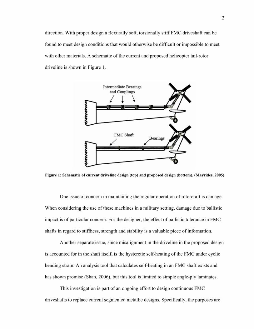
direction With proper design a flexurally soft torsionally stiff FMC driveshaft can be
found to meet design conditions that would otherwise be difficult or impossible to meet
with other materials A schematic of the current and proposed helicopter tail-rotor
driveline is shown in Figure 1
Figure 1 Schematic of current driveline design (top) and proposed design (bottom) (Mayrides 2005)
One issue of concern in maintaining the regular operation of rotorcraft is damage
When considering the use of these machines in a military setting damage due to ballistic
impact is of particular concern For the designer the effect of ballistic tolerance in FMC
shafts in regard to stiffness strength and stability is a valuable piece of information
Another separate issue since misalignment in the driveline in the proposed design
is accounted for in the shaft itself is the hysteretic self-heating of the FMC under cyclic
bending strain An analysis tool that calculates self-heating in an FMC shaft exists and
has shown promise (Shan 2006) but this tool is limited to simple angle-ply laminates
This investigation is part of an ongoing effort to design continuous FMC
driveshafts to replace current segmented metallic designs Specifically the purposes are
3
to contribute to design by means of material development investigate the effects of a
ballistic impact event on flexible matrix composites and refine analytical tools that
calculate the self-heating behavior in FMC driveshafts The objectives are summarized in
more detail following the literature review
4
Chapter 2 Literature Review
The current design for a driveline in rotorcraft consists of a series of aluminum
segmented shafts that are connected with flexible couplings and supported by hanger
bearings Flexible couplings are needed to account for the misalignment between the
main transmission and the tail rotor transmission Depending on the specific aircraft this
misalignment may be inherent or it could be due to aerodynamic and maneuvering loads
Due to fatigue limitations of metallic materials the design ensures there is no bending in
the aluminum segments and all of the misalignment in the driveline is accounted for in
the couplings Suggestions to improve this design have been to replace the aluminum
segments with rigid matrix composite (RMC) segments ndash the conventional structural
composite which is usually a carbonepoxy system (Darlow and Creonte 1995) There
were some weight savings in these studies but reduction in parts maintenance and
reliability was not observed A proposed design to improve and replace the segmented-
coupling design is one with a continuous FMC driveshaft (Hannibal and Avila 1984
Shan and Bakis 2005 Mayrides 2005) This design will reduce parts weight (Mayrides
et al 2005) and vibrations (DeSmidt 2005) and the high degree of anisotropy of FMCs
will allow for design parameters in stiffness to be met that would otherwise be difficult or
impossible to achieve with conventional RMCs
5
21 Flexible Matrix Composites
The term flexible matrix composites (FMCs) is used to identify composite
materials that are comprised of high strength high stiffness reinforcing fibers embedded
in a deformable flexible elastomeric polymer with a high yield strain and a glass
transition temperature that is usually significantly below ambient room temperature
Examples of these matrix materials include rubbers silicones and polyurethanes When
combined with the stiff reinforcing fibers the composite materials have very high
degrees of anisotropy because the stiffness of the material in the fiber direction can be
500 times greater (Shan 2002 Shan 2005) than the stiffness in the direction transverse to
the fibers This ratio for RMCs is typically around 20 (Daniel and Ishai 2006) Also the
ultimate transverse tensile strain of FMCs has been observed to be as high as 28 (Shan
2006) whereas for RMCs it is typically around 06 (Daniel and Ishai 2006) The
compressive strain at which fibers experience micro-buckling in FMCs has been
observed to be as low as 900 με (Shan 2006) whereas for RMCs it is typically around
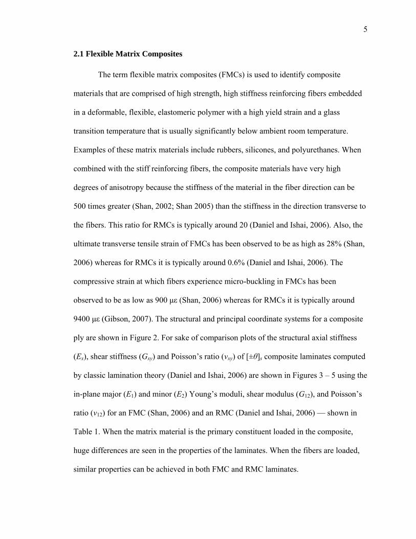
9400 με (Gibson 2007) The structural and principal coordinate systems for a composite
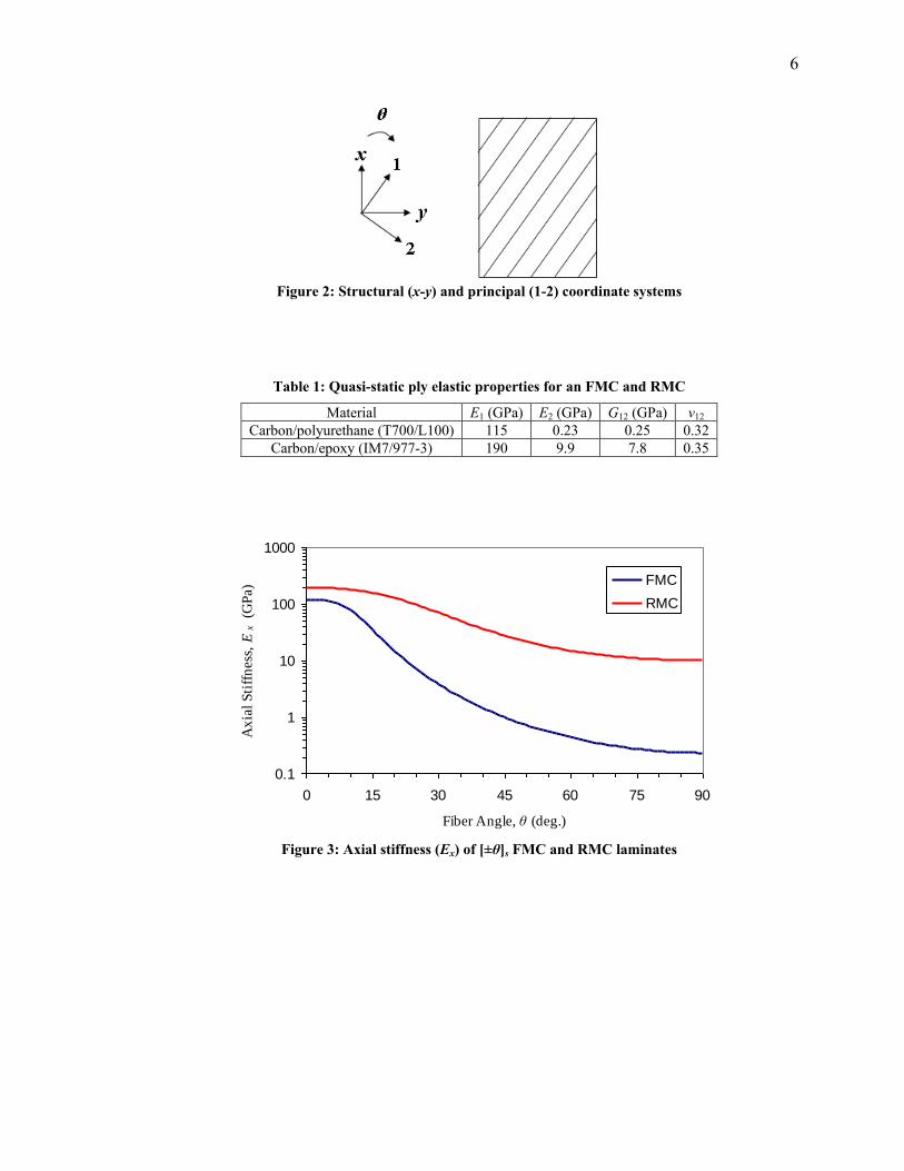
ply are shown in Figure 2 For sake of comparison plots of the structural axial stiffness
(Ex) shear stiffness (Gxy) and Poissonlsquos ratio (νxy) of [plusmnθ]s composite laminates computed
by classic lamination theory (Daniel and Ishai 2006) are shown in Figures 3 ndash 5 using the
in-plane major (E1) and minor (E2) Younglsquos moduli shear modulus (G12) and Poissonlsquos
ratio (ν12) for an FMC (Shan 2006) and an RMC (Daniel and Ishai 2006) mdash shown in
Table 1 When the matrix material is the primary constituent loaded in the composite
huge differences are seen in the properties of the laminates When the fibers are loaded
similar properties can be achieved in both FMC and RMC laminates
6
Figure 2 Structural (x-y) and principal (1-2) coordinate systems
Table 1 Quasi-static ply elastic properties for an FMC and RMC
Material E1 (GPa) E2 (GPa) G12 (GPa) ν12
Carbonpolyurethane (T700L100) 115 023 025 032
Carbonepoxy (IM7977-3) 190 99 78 035
01
1
10
100
1000
0 15 30 45 60 75 90
Fiber Angle θ (deg)
Ax
ial
Sti
ffn
ess
E
x (G
Pa) FMC
RMC
Figure 3 Axial stiffness (Ex) of [plusmnθ]s FMC and RMC laminates
7
01
1
10
100
0 15 30 45 60 75 90
Fiber Angle θ (deg)
Sh
ear
Sti
ffn
ess
G
xy (G
Pa)
FMC
RMC
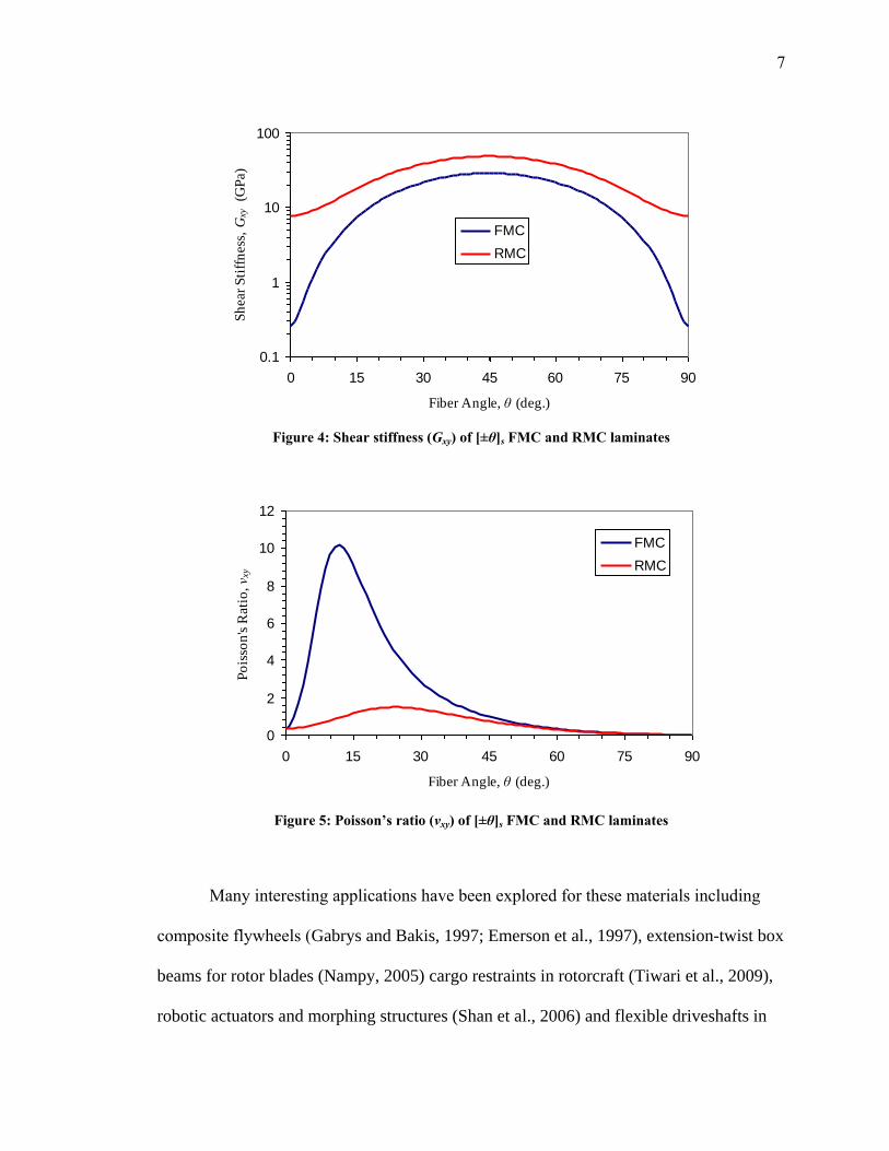
Figure 4 Shear stiffness (Gxy) of [plusmnθ]s FMC and RMC laminates
0
2
4
6
8
10
12
0 15 30 45 60 75 90
Fiber Angle θ (deg)
Po
isso
ns
Rati
o ν
xy
FMC
RMC
Figure 5 Poissonrsquos ratio (νxy) of [plusmnθ]s FMC and RMC laminates
Many interesting applications have been explored for these materials including
composite flywheels (Gabrys and Bakis 1997 Emerson et al 1997) extension-twist box
beams for rotor blades (Nampy 2005) cargo restraints in rotorcraft (Tiwari et al 2009)
robotic actuators and morphing structures (Shan et al 2006) and flexible driveshafts in
8
rotorcraft In the work on the internal heating behavior of FMC driveshafts (Shan and
Bakis 2002 Shan and Bakis 2009) a candidate material system was used for analysis
and experiments This system combined Toray T700 carbon fibers with a polyurethane
matrix made of Adiprenereg L100 prepolymer and Cayturreg 21 curing agent
22 Damage Tolerance in Fiber Reinforced Composites
A good deal of work has been done on examining the effects of impact damage in
RMCs over the years Most of the work focuses on carbonepoxy systems in a laminated
plate configuration Many advanced numerical simulations and analytical methods that
predict the effects of a ballistic impact event on a composite laminate have been
developed (Lee and Sun 1993 Silva et al 2005 Naik and Shrirao 2004) including
damage evolution damage size and the ballistic limit
Some investigators have studied the effects of impact damage on carbonepoxy
composite tubes (Christiansen et al 1988 Christoforou and Swanson 1988 Shivakumar
et al 1985 Valle 1989) Most of these investigations concentrate on the reduction in
strength due to low velocity impact which increases exponentially with increased area of
damage according to Valle (1989) Although a study conducted by Christiansen et al
(1988) using various impactors at hyper-velocity impact (4000 ndash 7500 ms) on
carbonepoxy tubes shows that projectile parameters such as size density velocity and
impact inclination have notable effects on target damage
The damage tolerance of carbonepoxy tubes made by hand layup with drilled
holes and medium-velocity (330 ndash 530 ms) impact damage loaded in compression was
studied by Ochoa et al (1991) at Texas AampM University The impact damage was
introduced by a 22 caliber rifle shot at normal and oblique angles to the composite tubes
9
Interestingly enough the compressive strengths after impact for the two tubes with
normal and oblique impact damage were no different Also the reported reduction in
strength due to the ballistic impact was equal to the reduction in strength due to a drilled
hole with a diameter that is 50 of the tube diameter (22 caliber projectile diameter is
55 of tube diameter) This ratio (drilled hole or projectile diameter to tube diameter) is
referred to as the hole-tube ratio dhdt Ochoa et al (1991) report that for dhdt values of
013 and 050 knockdowns in compressive strength for carbonepoxy tubes were 52
and 78 respectively Tubes in this investigation had an outer diameter of 1016 cm a
wall thickness of 140 mm and a stacking sequence of [plusmn18902plusmn18902plusmn18]
A study on the failure mode of carbonepoxy tubes made by hand layup with
drilled holes in torsion was performed by Bauchau et al at Rensselaer Polytechnic
Institute (1988) In this study the authors concluded that the failure mode for tubes that
had dhdt values of 030 ndash 046 was torsional buckling When this ratio increased to 060
the mode observed was material failure This trend was observed for tubes with outer
diameters of about 42 mm wall thicknesses of about 11 mm and two different stacking
sequences of [15-15-45-151545] and [4515-15-45-1515]
The effect of drilled holes as stress concentrations in filament-wound flexible
matrix composite tubes was examined by Sollenberger et al (2009) In this case the
quasi-static moduli and strength of notched and unnotched tubes were compared in
tension and compression For dhdt values of 025 and 030 the maximum knockdowns in
compression strength (multiple layups) for the carbonflexible epoxy tubes were 25 and
40 respectively Different angle-ply layups were tested from plusmn23deg to plusmn90deg with the
hoopwound configuration seeing the maximum knockdown The plusmn23deg configuration saw
knockdowns of only 5 and 13 The outer diameter of these tubes was about 22 mm and
10
wall thicknesses were about 1 mm Although it is recognized that the geometries layups
and stacking sequences are quite different in the two studies of RMCs (Ochoa et al
1991) and FMCs (Sollenberger et al 2009) in regard to the drilled hole-tube ratio the
knockdowns in compression strength for the rigid matrix composites seem to be higher
than those for the flexible matrix composites Fatigue testing of FMC tubes subjected to
over 3 million cycles with drilled holes was also performed by Sollenberger et al (2009)
Using X-radiography the author found no observable fatigue crack growth
23 Calculating Temperature Increase due to Hysteresis
Flexible matrix composite driveshafts that are misaligned and rotating experience
self-heating due to hysteretic damping and cyclic bending strain Most of the damping
occurs in the polymer matrix material although as pointed out by many investigators
(eg Gibson et al 1982) fibers do have a small amount of damping that contribute to the
overall damping of the composite Hysteretic damping refers to the behavior in materials
where the resultant force lags behind the applied strain In each cycle of loading a finite
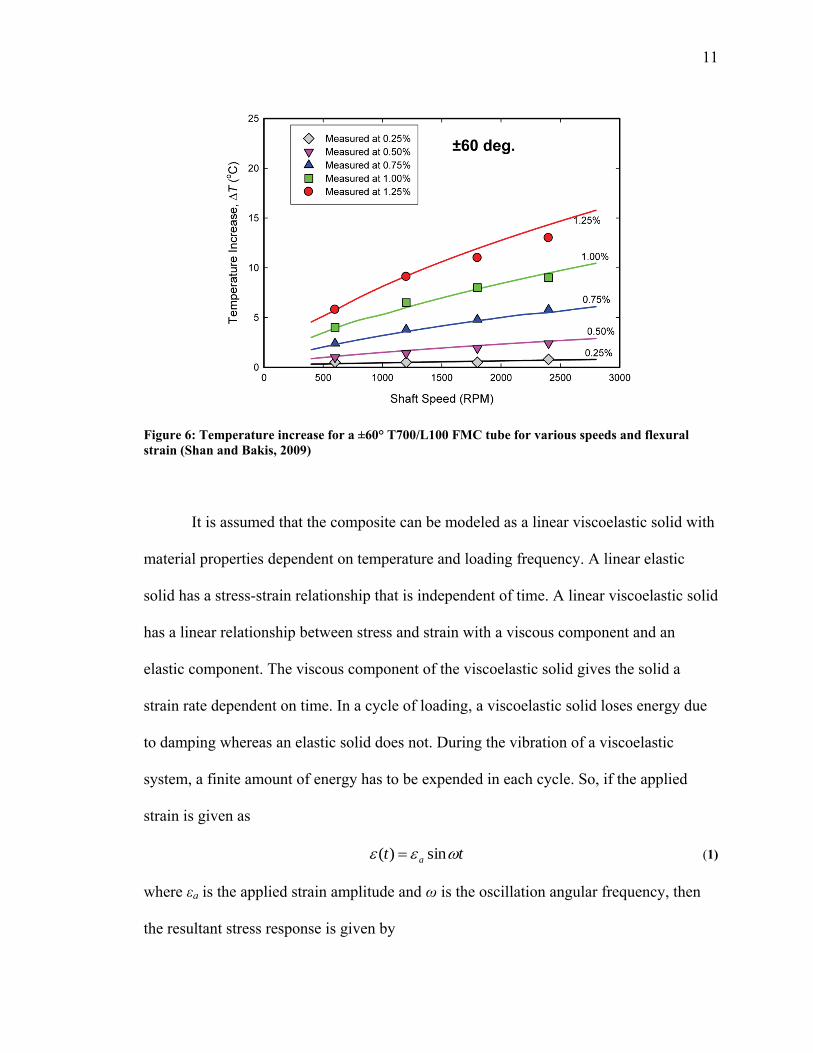
amount of energy is lost as heat due to damping A thermomechanical model that
calculates self-heating in FMC driveshafts has been developed (Shan and Bakis 2009)
and shows good correlation with experimental results mdash shown in Figure 6 Since the
self-heating model agrees well with experimental data the approach to model and
measure the damping behavior of FMCs is chosen to be the same in the current work A
review of some of the most common material damping models is given here ndash including
the specific damping models used in the work of Shan and Bakis (2009)
11
Figure 6 Temperature increase for a plusmn60deg T700L100 FMC tube for various speeds and flexural
strain (Shan and Bakis 2009)
It is assumed that the composite can be modeled as a linear viscoelastic solid with
material properties dependent on temperature and loading frequency A linear elastic
solid has a stress-strain relationship that is independent of time A linear viscoelastic solid
has a linear relationship between stress and strain with a viscous component and an
elastic component The viscous component of the viscoelastic solid gives the solid a
strain rate dependent on time In a cycle of loading a viscoelastic solid loses energy due
to damping whereas an elastic solid does not During the vibration of a viscoelastic
system a finite amount of energy has to be expended in each cycle So if the applied
strain is given as
tt a sin)( (1)
where εa is the applied strain amplitude and ω is the oscillation angular frequency then
the resultant stress response is given by
12
)sin()( tt a (2)
where ζa is the resultant stress amplitude and is the phase angle difference between the
applied strain and resultant stress For an elastic material the phase difference between
the stress and strain is zero For a viscoelastic material is non-zero The work done
per cycle is then
sin)()()()(2
0
aadttttdtW (3)
and the maximum strain energy in the system can be defined as half the product of the
maximum strain and the corresponding instantaneous value of stress
cos2
1)
2sin(
2sin
2
1
aaaaW (4)
The loss factor is then defined by
tan2
1
W
W (5)
which is a measure of the energy lost during each cycle The loss factor can be
determined by measuring the phase difference between the sinusoidal waveforms of the
applied strain and the resulting stress This approach to measuring the loss factor is called
the phase lag method and is described by Kinra and Wren (1992a 1992b) An FFT
analysis is done on the waveforms to determine the phase difference
Another result of the phase lag method is the complex modulus ndash which relates
the applied strain to the resultant stress The complex modulus is comprised of two parts
the storage modulus and the loss modulus The storage modulus is a measurement of the
ratio of the in-phase resultant stress to the applied strain The loss modulus is a
measurement of the out-of-phase ratio of the resultant stress to the applied strain Using
trigonometric identities Equation 2 can be re-written as
13
sincoscossin)( ttt aa (6)
From Equation 6 it is clear that the stress is resolved into two quantities one that is in
phase with the applied strain and one that is out of phase with the applied strain These
quantities can be related to the storage and loss moduli by Equations 7 and 8
respectively
cos
a
aE (7)
sin
a
aE (8)
Hence Equation 6 can be re-written as
aaaa EiEEtEtEt )(cossin)( (9)
where E is called the complex modulus By dividing Equation 8 by Equation 7 one
obtains the loss factor
tan
E
E (10)
Complex moduli can be determined from the phase lag method but also from methods
like the forced vibration of a cantilever beam (viscoelastic flexural modulus) where the
phase angle by which the tip deflection of the beam lags behind the displacement of a
shaker at the base measures damping (Paxson 1975)
Other measures of damping include the logarithmic decrement δ which is a
measure of the exponential free decay of oscillation with time in a damped system It is
determined by the free vibration method which measures the decay in the vibration
amplitude of an initially excited cantilever beam (Paxson 1975 Chandra et al 2003)
Some researchers use the inverse quality factor Q-1
which relates to the steady state
14
amplitude attained by a structure excited by a harmonically oscillating force It is
determined by
121
n
Q
(11)
where ωn is the resonant frequency and ω1 and ω2 are the frequencies on either side of ωn
for which the response amplitude is 21 times the resonant amplitude ndash ie the half
power points The inverse quality factor can determined by the impulse technique where
a transfer function for the specimen is found by tapping a beam or a cubic specimen with
a hammer which has a force transducer attached to its head A motion transducer is used
to measure the response of the specimen The signals from the two transducers are fed
into an FFT analysis to determine the response versus frequency The inverse quality
factor Q-1
is obtained by using half-power-band-width technique (Suarez et al 1984
Crane and Gillespie 1991 Chandra et al 2003) The inverse quality factor can also be
determined from the torsional vibration method (Adams et al 1969 White and Abdin
1985) where a composite rod is undergoing steady state torsional vibration A vibrational
load is applied to the bar by a two coil-magnet system undergoing an alternating current
The alternating current is compared to the response from the surface strain gages and the
damping is determined by Equation 11
In order to accurately represent the behavior of the matrix-dominated properties
of the composite for ranging frequencies a fractional derivative model (Bagley and
Torvik 1979 Bagley and Torvik 1983 Papoulia and Kelly 1997 Rogers 1983) was
used by Shan and Bakis (2009) The fractional derivative model is a variation from the
standard linear model or the Zener model (Nashif et al 1985 Ferry 1970) Instead of the
classic representation of the state equation between σ and ε which is given by
15
dt
dbEE
dt
da
(12)
the integral derivatives are replaced by fractional derivatives
)()()()( tDbEtEtDat (13)
where 0ltβlt1 and the fractional derivative of order β is defined as
t
dt
x
dt
dtxD
0
)(
)(
)1(
1)]([
(14)
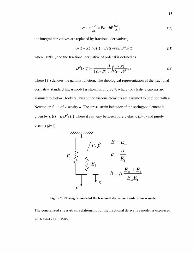
where Γ(middot) denotes the gamma function The rheological representation of the fractional
derivative standard linear model is shown in Figure 7 where the elastic elements are
assumed to follow Hookelsquos law and the viscous elements are assumed to be filled with a
Newtonian fluid of viscosity μ The stress-strain behavior of the springpot element is
given by )()( tDt where it can vary between purely elastic (β=0) and purely
viscous (β=1)
Figure 7 Rheological model of the fractional derivative standard linear model
The generalized stress-strain relationship for the fractional derivative model is expressed
as (Nashif et al 1985)
ζ ε
E1
E
唴
_
μ β
1Ea
1
1
EE
EEb
EE
16
)()()(11
tDbEEtDat kk
n
k
k
n
k
k
(15)
For a harmonic response of the form tie 0 and tie 0 Equation 15 gives
)(1
)(1
1
100
k
k
ia
ib
En
k
k
n
k
k
(16)
So the storage and loss moduli are
E
ia
ib
Ek
k
n
k
k
n
k
k
)(1
)(1
Re
1
1 (17)
E
ia
ib
Ek
k
n
k
k
n
k
k
)(1
)(1
Im
1
1 (18)
In order to account for the differences in storage and loss moduli throughout
varying temperature ranges the temperature-frequency superposition principle (Ferry
1970) is used (Shan and Bakis 2009) Temperature shifting factors translate storage
modulus and loss factor curves versus frequency at different temperatures toward a
reference temperature into one master curve The master curve contains information for
the complex modulus at different temperatures and frequencies To model damping in the
composite a macro-mechanical strain energy method developed by Adams et al (Adams
and Bacon 1973a 1973b Ni and Adams 1984) was used in the work of Shan and Bakis
(2009) to calculate the dissipated strain energy If the overall damping in the composite is
a sum of all of the strain energy losses from each of the elements of the composite then
the overall dissipated strain energy is represented by
17
2 i
ii
i
i WW (19)
where the index i represents the individual elements of the composite Contributions from
the three normal and in-plane shear stresses and strains were included in the
thermomechanical model (Shan and Bakis 2009)
Other methods to model damping in composites include the viscoelastic
correspondence approach first proposed by Hashin (Hashin 1970a Hashin 1970b)
which says that a quasi-static linear viscoelastic analysis can be converted to a dynamic
linear viscoelastic analysis by replacing static stresses and strains with the corresponding
dynamic stresses and strains and by replacing elastic moduli with complex moduli
Micro-mechanical approaches to model damping in composites have been also been
examined that model damping mechanisms on the fibermatrix level Many of these
models have examined short fiber reinforced composite material (Gibson et al 1982
Sun et al 1987 White and Abdin 1985) but some have also modeled continuous fiber
reinforced materials (Caruso and Chamis 1986 Saravanos and Chamis 1992) The
continuous fiber models include fiber matrix and volume fraction properties They also
predict damping behavior of the composite based on temperature absorbed moisture
fibermatrix interface friction and fiber breakage
24 Limitations of Previous Work
Although the flexible matrix material ndash Adiprenereg L100 ndash used in Shan and
Bakis (2002 2009) exhibited good dynamic and fatigue behavior experimental and
design work at Penn State has shown that this system may be too soft for an actual shaft
application Some testing and analytical work revealed the onset of fiber micro-buckling
to be about 900 με (Shan 2006) This is a failure mode that jeopardizes the stiffness of
18
the composite and is the result of fibers being loaded in compression while being
supported by a soft matrix Designing with the L100 system would require a thick-
walled heavy shaft This is not ideal when the goal of the design is to minimize weight
The micro-buckling strain and weight issues certainly have an adverse effect on design
and a stiffer matrix may improve the end result A stiffer matrix material with a flexible
epoxy formulation was used in studying the effect of stress concentrations in FMCs
(Sollenberger et al 2009) but upon further inspection the dynamic behavior of the
flexible epoxy chemistry turned out to have major disadvantages The matrix was
overdamped and exhibited a large increase in stiffness with increasing frequency For
these reasons the possibility of testing and designing with a stiffer polyurethane matrix is
an attractive option This approach would maintain the good dynamic properties of the
Adiprenereg L100 system while alleviating some of the issues of the very soft and
compliant matrix Because many design such as heating strength buckling and whirl
instability of the shaft constraints are dependent on material properties material selection
and property determination is an important task and is pursued here
As far as the author knows all of the previous work on ballistic testing of
composites has been carried out with RMC systems like carbonepoxy and glassepoxy
For this reason the ballistic tolerance of FMC materials will be investigated here
Damage tolerance in FMC tubes was studied in Sollenberger et al (2009) but it was
limited to drilled holes A drilled hole does not necessarily represent the damage due to a
ballistic impact event The dynamics of a high velocity impact can cause material to
deform and fracture in ways that are highly unpredictable In this work (Sollenberger et
al 2009) the post-impact testing was also limited to quasi-static tension and
compression and a bending fatigue test So in the current work the effect of ballistic
19
damage on the quasi-static torsional strength of a small-scale FMC tube will be studied in
addition to quasi-static tension and compression along with bending fatigue Since torsion
is the primary quasi-static loading case of a driveshaft this effect will be of key interest
The thermomechanical model that predicts the steady state temperature of a
rotating misaligned composite shaft developed by Shan and Bakis (2009) is limited to
one fiber angle in the layup sequence In the optimization work of Mayrides (2005) it was
found that layups with more than one angle were sometimes preferred So an
improvement to Shan and Bakislsquos (2009) analysis tool that allows for the calculation of
self-heating in a multi-angled tube seems to be relevant and is pursued Also a finite
element model that calculates self-heating in an FMC driveshaft could easily model
multi-angled layups and could prove to be valuable when considering FMC shaft design
in industry With a framework to calculate self-heating in finite elements aspects of FMC
shaft design like bearing support and complicated misalignment loadings could be
introduced with some minor additional effort For these reasons the development of a
finite element model is also pursued in the present investigation
25 Problem StatementResearch Goal
The objectives of the current investigation are to characterize the material
property parameters of a stiff carbonpolyurethane composite characterize the ballistic
tolerance of FMC tubes and improve and add to analytical tools used to calculate self-
heating in FMC driveshafts A stiff polyurethane may simultaneously reduce the weight
of an optimized FMC driveshaft in a final design while keeping the superior dynamic
behavior observed in previous research Although the actual design of an FMC shaft for
a rotorcraft is beyond the scope of the present investigation Characterizing the ballistic
20
tolerance of FMC tubes will provide preliminary information about how an FMC
driveshaft may perform during and after an impact event in service As far as the author
knows testing the ballistic tolerance of flexible matrix composite materials is unique
Because design tools have suggested optimized layups that contain multiple fiber angles
an improvement on the established analytical tool to calculate heating in FMC driveshafts
to include these conditions is considered worthwhile and relevant These objectives will
be achieved by the following task list
1 Select an appropriate material system on which to perform quasi-static and
dynamic testing for material property characterization
2 Perform ballistic testing on filament-wound tube coupons to determine the
effects of a ballistic impact event on FMC tubes
3 Alter the existing thermomechanical model that calculates self-heating of
undamaged FMC driveshafts to include multi-angled layups Also
develop a finite element model to calculate the self-heating
4 Carry out quasi-static and dynamic testing on FMC materials to determine
the material properties need to predict the quasi-static and self-heating
behavior of FMC tubes
5 Use the material property parameters and the self-heating models to
compare the calculations of self-heating (from models) and the
measurements of self-heating (from experiments) for undamaged FMC
tubes
The following chapters describe the approach of the current investigation
Materials and fabrication methods are covered in Chapter 3 Chapter 4 covers ballistic
testing quasi-static testing and quasi-static material property determination Note that
21
Chapter 4 is the only chapter addressing ballistic testing Chapter 5 describes dynamic
testing and material property determination Chapter 6 reviews the self-heating results
from the models and experiments Finally conclusions and recommendations for future
work are given in Chapter 7 Computer codes used in the current research a sensitivity
analysis and a few relevant videos are given in the appendices
22
Chapter 3 Materials and Fabrication Methods
For this investigation carbon fiber reinforced composites with a rigid matrix
material and a flexible matrix material were fabricated so that comparisons in
performance between RMCs and FMCs can be made The rigid matrix material in the
RMCs is an epoxy while the flexible matrix material in the FMCs is a flexible
polyurethane (described later) Tubes will be used to describe small hollow cylindrical
test coupons and shafts will be used to describe a cylindrical fully-designed load-bearing
structure in this thesis Filament-wound tubes were made for spin testing ballistic testing
as well as quasi-static and dynamic material property characterization Flat plate coupons
were also made by filament winding for additional dynamic material property
characterization For flat plate coupons instead of winding wet carbon tows onto a
cylindrical mandrel (as in tube fabrication) the tows were wound onto a flat steel plate to
create unidirectional composite plies These plies were then cut and arranged in a closed
mold and cured in a hot-press
The filament winding process is a method of fabricating fiber reinforced polymer
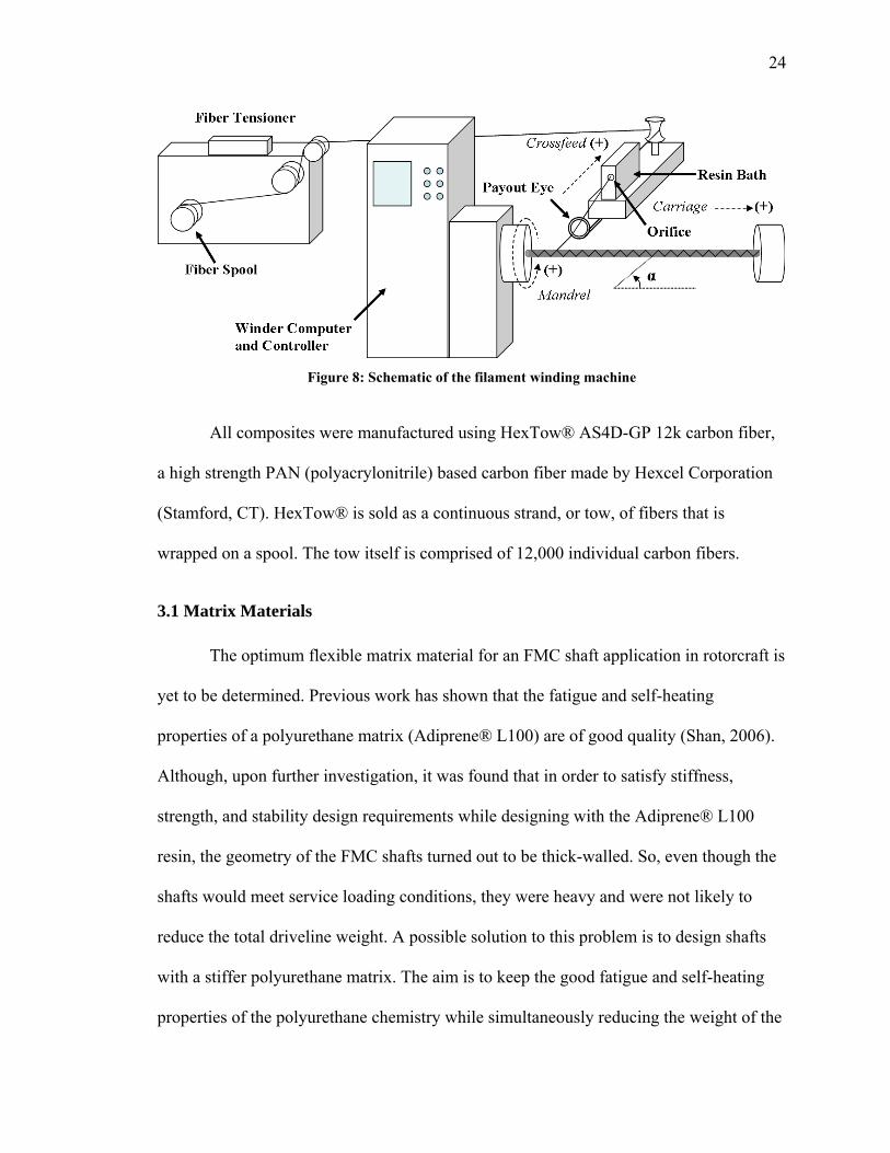
composites A schematic of the filament winding process can be seen in Figure 8 To
start the carbon fiber tow unwinds from the original fiber spool The tow then runs over a
set of two pulleys that are attached to the fiber tensioning machine The normal force
exerted on these pulleys from the tow is used as feedback information for the tensioner so
23
that it can apply the constant user-defined amount of tension on the tow The tow then
makes a turn at the rear end of the crossfeed just before it enters the first orifice in the
resin bath The first orifice is usually selected to be considerably larger than the second
because it does not affect the amount of resin that is impregnated into the tow ndash a major
factor affecting the final fiber volume fraction of the part Once the tow enters the resin
bath it is spread out on three polished static rods while simultaneously being immersed
in the liquid resin The spreading of the tow ensures proper impregnation When the tow
leaves the resin bath a prescribed amount of the impregnated resin is squeezed out of the
tow by the second orifice The size of the second orifice is selected to achieve the
appropriate fiber volume fraction in the composite Once the tow leaves the resin bath it
is fed through the payout eye The payout eye lays the wet tow onto the mandrel in the
proper position The linear speed at which the carriage moves relative to the rotational
speed of the mandrel dictates the fiber winding angle which is shown as α in Figure 8
Once the mandrel is completely covered with the composite material it is wrapped with a
heat shrinking tape that consolidates the part during cure The mandrel with the
composite and shrinking tape is then transported to an oven for curing Once the
composite is cured the tape is removed from the composite and the composite is
removed from the mandrel
24
Figure 8 Schematic of the filament winding machine
All composites were manufactured using HexTowreg AS4D-GP 12k carbon fiber
a high strength PAN (polyacrylonitrile) based carbon fiber made by Hexcel Corporation
(Stamford CT) HexTowreg is sold as a continuous strand or tow of fibers that is
wrapped on a spool The tow itself is comprised of 12000 individual carbon fibers
31 Matrix Materials
The optimum flexible matrix material for an FMC shaft application in rotorcraft is
yet to be determined Previous work has shown that the fatigue and self-heating
properties of a polyurethane matrix (Adiprenereg L100) are of good quality (Shan 2006)
Although upon further investigation it was found that in order to satisfy stiffness
strength and stability design requirements while designing with the Adiprenereg L100
resin the geometry of the FMC shafts turned out to be thick-walled So even though the
shafts would meet service loading conditions they were heavy and were not likely to
reduce the total driveline weight A possible solution to this problem is to design shafts
with a stiffer polyurethane matrix The aim is to keep the good fatigue and self-heating
properties of the polyurethane chemistry while simultaneously reducing the weight of the
25
final optimally designed shaft A stiffer matrix material will not require such a thick wall
to meet all of the design requirements although it may generate more hysteretic heating
than a softer matrix
The Chemtura Corporation (Middlebury CT) was consulted for material
development and they suggested Adiprenereg LF750D a liquid polyether prepolymer
They also suggested using a curative with this prepolymer called Cayturreg 31 DA a
delayed-action diamine curative The polymer is made by mixing the prepolymer and the
curative at a mass mixing ratio of 100 503 This mixture is then heated to 140degC for 2
hours followed by a 16 hour post-cure at 100degC Cayturreg 31 DA is described as a
delayed-action curative because at room temperature it is nearly non-reactive However
when Cayturreg 31 DA is heated to 115 ndash 160degC the salt complex in the curative dissolves
which frees the methylene dianiline (MDA) complex The MDA then reacts quickly with
the toluene diisocyanate (TDI) terminated prepolymer to form an elastomeric
polyurethane (Chemtura 2007) The temperature of the resin bath during fabrication was
kept at 50degC to reduce viscosity Since this stiffer polyurethane may show promise in
designing FMC shafts for operational rotorcraft it will be used for all testing of flexible
matrix composites in this investigation A sample sheet of the cured polyurethane was
provided by Chemtura for material property evaluation
Another research goal for the current investigation is to make a comparative
examination between the ballistic tolerance of RMCs and FMCs For the rigid matrix
composites a low viscosity liquid epoxy resin system was selected for use because of its
availability and good processing characteristics The rigid matrix material is made by
combining EPONtrade 862 a liquid bisphenol A epoxide made by Hexion Specialty
Chemicals Inc (Columbus OH) with Baytec Curative W a liquid aromatic diamine
26
curative also made by Hexion with a mass mixing ratio of 100 264 This mixture is
heated to 121degC for a 1 hour soak followed by a 2 hour cure at 177degC The resin bath was
kept at room temperature during fabrication
32 Tube Fabrication
Small-scale FMC and RMC composite tubes were made by the wet filament
winding fabrication process on a McLean-Anderson Filament Winder photographs of
which can be seen in Figure 9 Before winding a target fiber volume fraction Vft is
chosen to calculate the size of the orifice on the resin bath The relationship between
target fiber volume fraction and orifice diameter Do is calculated as follows
2
2
o
ff
ftD
NDV
(20)
where Df is the diameter of the fibers and Nf is the number of fibers per tow For a target
fiber volume fraction of 060 calculations indicate a 0940 mm (0037 in) diameter
orifice for 12K (12000 filaments) tow with a fiber diameter of 67 μm (Hexcel 2009)
Due to limitations on orifice selection a 0965 mm (0038 in) diameter orifice is used
which provides a volume fraction of 058 The actual fiber volume fraction of the
specimen after it is cured Vfa is calculated using the following equation
tb
DNNV
w
ffp
fa
2
2
(21)
where Np is the number of plies bw is the programmed bandwidth of each tow and t is the
total thickness of the wound part following cure Each coverage of a helically wound tube
is considered to be 2 layers for this calculation
27
Figure 9 Filament winder overview (left) and detailed view (right)
Two different sized mandrels were used for tube fabrication A solid steel
mandrel with a 1984 mm outer diameter is used to make tubes for spin testing ballistic
testing and quasi-static material property characterization A smaller solid steel mandrel
with an outer diameter of 991 mm was used to make FMC tubes for dynamic material
property measurements Both mandrels have tapped holes on either end so that end plugs
can be attached These end plugs then interface with and are gripped by the two chucks
on the filament winder From now on tubes with winding angles between 0deg and 60deg will
be referred to as helical tubes while tubes with a winding angle of 0deg will be referred to
as unidirectional tubes and tubes with a winding angle close to 90deg will be referred to as
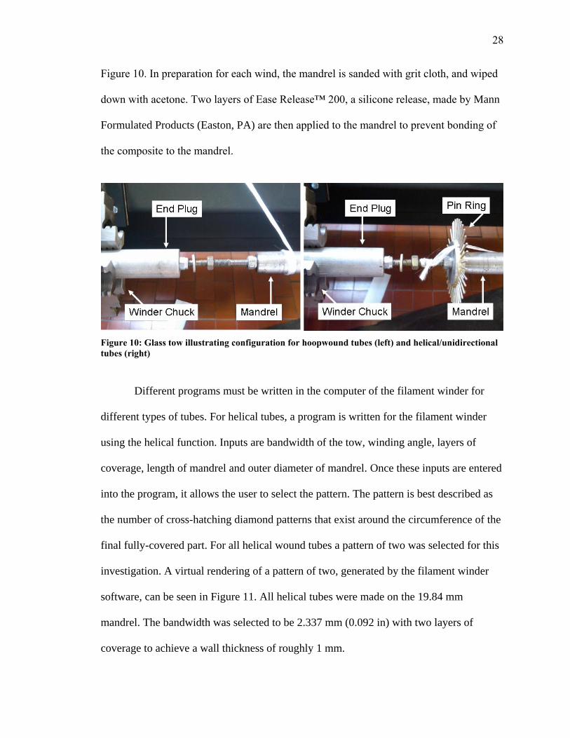
hoopwound tubes For helical and unidirectional tubes pin rings are used on the end
plugs (Figure 10) Pin rings eliminate the sharp curvature of the end of the cylindrical
mandrel which could fray the fibers and lead to tow breakage and they provide a
hooking point at the end of the mandrel so that the tow does not slip ndash a feature that is
particularly important and useful for fiber winding angles less than 30deg The winding
angle for hoopwound tubes is very close to 90deg but is always slightly less An illustration
of the hoopwound configuration and the helicalunidirectional configuration is shown in
28
Figure 10 In preparation for each wind the mandrel is sanded with grit cloth and wiped
down with acetone Two layers of Ease Releasetrade 200 a silicone release made by Mann
Formulated Products (Easton PA) are then applied to the mandrel to prevent bonding of
the composite to the mandrel
Figure 10 Glass tow illustrating configuration for hoopwound tubes (left) and helicalunidirectional
tubes (right)
Different programs must be written in the computer of the filament winder for
different types of tubes For helical tubes a program is written for the filament winder
using the helical function Inputs are bandwidth of the tow winding angle layers of
coverage length of mandrel and outer diameter of mandrel Once these inputs are entered
into the program it allows the user to select the pattern The pattern is best described as
the number of cross-hatching diamond patterns that exist around the circumference of the
final fully-covered part For all helical wound tubes a pattern of two was selected for this
investigation A virtual rendering of a pattern of two generated by the filament winder
software can be seen in Figure 11 All helical tubes were made on the 1984 mm
mandrel The bandwidth was selected to be 2337 mm (0092 in) with two layers of
coverage to achieve a wall thickness of roughly 1 mm
29
Figure 11 Illustration of two cross-hatching diamond patterns around the circumference of a
filament-wound tube
For unidirectional tubes since all of the fiber tows are oriented in the axial
direction of the cylindrical mandrel the carriage moves from one end of the mandrel to
the other while the mandrel remains stationary The mandrel rotates (through its index)
only while the carriage dwells at one end or the other The inputs for writing a
unidirectional program are length and outer diameter of the mandrel index number of
strokes and the plunge distance The index ι is measured in degrees and is expressed as
follows
S
360360 (22)
where S is the number of strokes The number of strokes is how many total times the
winder traverses the mandrel In a unidirectional wind the winder lays tows sequentially
next to one another until the entire mandrel is covered The plunge distance is how far the
crossfeed moves in toward the mandrel when the carriage is located at either end of the
mandrel This translation of the crossfeed allows the pin rings to hook the tow at the ends
of the mandrel after each pass All unidirectional tubes were made on the 991 mm
mandrel with an index of 3667deg and 54 strokes totaling one layer
30
For hoopwound tubes the inputs to the program are bandwidth of the tow layers
of coverage length of mandrel and outer diameter of mandrel The bandwidth of the tow
for hoopwound tubes was also selected to be 2337 mm (0092 in) All hoopwound tubes
were made on the 1984 mm mandrel with four layers of coverage to achieve a wall
thickness of roughly 1 mm The actual fiber angle of the hoopwound tubes in this
investigation was 832deg
For all tube types a tension force of 445 N was applied to the tow All helical
and hoopwound tubes were wound on the 1984 mm mandrel while all unidirectional
tubes were wound on the 991 mm mandrel Two different angles were wound with the
carbonepoxy system (Table 2) Six different fiber angles were wound with the
carbonpolyurethane system (Table 3) Measured geometric properties of the tubes after
cure and the actual (calculated) fiber volume fractions (assuming no voids) for the
carbonepoxy and carbonurethane tubes are shown in Table 2 and in Table 3 The inner
diameters of the plusmn60deg and plusmn832deg tubes are slightly larger than the mandrel size which is
a consequence of the dependence of the thermal expansion characteristics of the tubes on
the fiber winding angle
Table 2 Geometric properties and fiber volume fractions of the carbonepoxy tubes
Fiber Angle
(deg) plusmn 45deg plusmn 60deg
ID (cm) 198 198
OD (cm) 221 221
Cross-sectional
Area (mm2) 75 74
Vfa 064 063
31
Table 3 Geometric properties and fiber volume fractions of the carbonpolyurethane tubes
Fiber Angle
(deg) plusmn 20deg plusmn 30deg plusmn 45deg plusmn 60deg plusmn 832deg 0deg
ID (cm) 198 198 198 199 199 0991
OD (cm) 222 223 223 223 224 1201
Cross-sectional
Area (mm2) 80 80 83 79 84 36
Vfa 059 060 058 059 058 065
After the filament winder finished covering the mandrel the program was stopped
and shrink-tape was wrapped around the specimen in order to help consolidate the
composite and provide a smooth finish The shrink-tape is called Hi-Shrink Tape
Release Coated (25 mm wide 005 mm thick 80degC activation temperature) from
Dunstone Inc (Charlotte NC) Careful attention must be paid to the tension on the tape
the angle at which it is applied and the width of the tape versus over-lap width when
being applied This idea is more clearly understood by examining Figure 12 Over-lap
width was selected to be roughly half the width of the shrink-tape
Figure 12 Shrink tape application
After the tubes were cured and the shrink tape was removed the tubes were
pulled off the mandrel The ends were cut off using a water-cooled circular saw with a
diamond tipped blade and discarded The 1984 mm sized tubes were 90 cm in length
From the 90 cm tubes 76 cm sections were cut for compression testing 127 cm sections
32
were cut for tension and torsion testing and 457 cm sections were cut for spin testing
The 991 mm mandrels were 38 cm in length From the 38 cm tubes 25 mm sections
were cut for torsional dynamic mechanical analysis
33 Flat Plate Fabrication
Flat plate coupons were made for dynamic material property characterization for
the FMC material Pre-impregnated sheets of carbon fiber (referred to as pre-preg sheets
or simply pre-pregs from now on) were made by using the wet filament winding process
much the same way tubes are made Instead of winding the wet tow onto a cylindrical
mandrel the tow was wound onto a flat mandrel To generate motion of the machine a
circumferential (hoopwound) winding program was chosen Since the flat mandrel is not
cylindrical in shape the diameter input is nonsensical So a diameter was chosen such
that the distance that the tow will travel while winding around the flat mandrel (the
perimeter) is equal to the circumference of an imaginary cylindrical mandrel Selecting
the diameter and bandwidth properly ensured that fibers were spaced appropriately with
no gaps The diameter and bandwidth used were 194 cm and 2337 mm respectively A
photograph of the set-up used to wind pre-preg sheets of carbon fiber is shown in Figure
13 In this photograph the carriage is hidden behind the flat mandrel and the program has
just started its first circuit
33
Figure 13 Winding onto a flat plate mandrel to make pre-impregnated sheets of carbon fiber
Two layers of coverage were used to cover the flat mandrel For a circumferential
wind one layer of coverage is defined as a sweep of the carriage from the headstock to
tailstock Once the flat mandrel was covered it and the composite material wound onto it
were placed between two pressure platens so that the continuous strands could be cut on
the edges of the flat mandrel ndash resulting in two sheets of pre-preg These two sheets of
pre-preg were roughly 20 x 28 cm in size Because the closed steel mold used to cure the
flat plate coupons is roughly 10 x 56 cm in size the two sheets of pre-preg were cut in
half and stacked on top of one another so they fit the mold The broken-fiber seam at the
mid-length position of themold was excluded from the testing program This process is
summarized in Figure 14
34
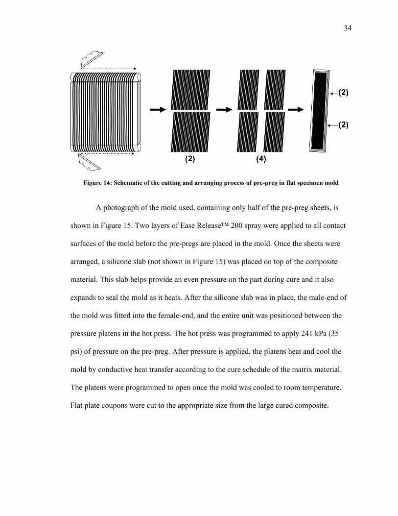
Figure 14 Schematic of the cutting and arranging process of pre-preg in flat specimen mold
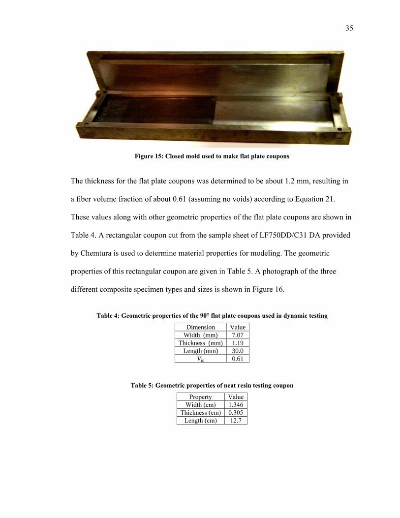
A photograph of the mold used containing only half of the pre-preg sheets is
shown in Figure 15 Two layers of Ease Releasetrade 200 spray were applied to all contact
surfaces of the mold before the pre-pregs are placed in the mold Once the sheets were
arranged a silicone slab (not shown in Figure 15) was placed on top of the composite
material This slab helps provide an even pressure on the part during cure and it also
expands to seal the mold as it heats After the silicone slab was in place the male-end of
the mold was fitted into the female-end and the entire unit was positioned between the
pressure platens in the hot press The hot press was programmed to apply 241 kPa (35
psi) of pressure on the pre-preg After pressure is applied the platens heat and cool the
mold by conductive heat transfer according to the cure schedule of the matrix material
The platens were programmed to open once the mold was cooled to room temperature
Flat plate coupons were cut to the appropriate size from the large cured composite
35
Figure 15 Closed mold used to make flat plate coupons
The thickness for the flat plate coupons was determined to be about 12 mm resulting in
a fiber volume fraction of about 061 (assuming no voids) according to Equation 21
These values along with other geometric properties of the flat plate coupons are shown in
Table 4 A rectangular coupon cut from the sample sheet of LF750DDC31 DA provided
by Chemtura is used to determine material properties for modeling The geometric
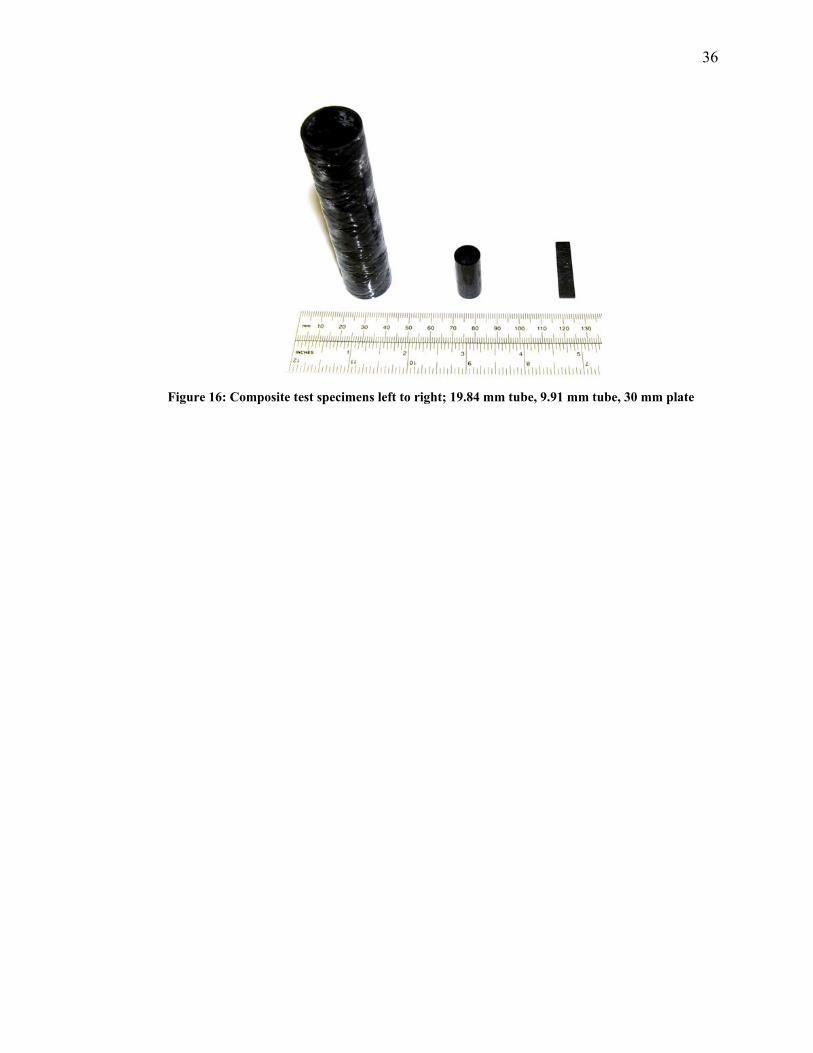
properties of this rectangular coupon are given in Table 5 A photograph of the three
different composite specimen types and sizes is shown in Figure 16
Table 4 Geometric properties of the 90deg flat plate coupons used in dynamic testing
Dimension Value
Width (mm) 707
Thickness (mm) 119
Length (mm) 300
Vfa 061
Table 5 Geometric properties of neat resin testing coupon
Property Value
Width (cm) 1346
Thickness (cm) 0305
Length (cm) 127
36
Figure 16 Composite test specimens left to right 1984 mm tube 991 mm tube 30 mm plate
37
Chapter 4 Ballistic Tolerance and Determination of Quasi-Static Properties
Several test methods and test results are described in this chapter The ballistic
impact testing of FMC and RMC materials is discussed first The stress-strain behavior of
damaged and undamaged tubes is discussed next This behavior provides a means to
quantify ballistic tolerance Also analysis of the quasi-static stress-strain behavior of
undamaged flexible carbonpolyurethane composites yields ply elastic properties that
characterize the composite material Dynamic material properties are presented in
Chapter 5
41 Ballistic Impact Testing
FMC and RMC tubes of the 20 mm inner diameter type were used to characterize
the ballistic tolerance of flexible and rigid matrix composites The composite tubes were
impacted with a steel ball bearing fired from a pressurized air gun In this section the
impact testing set-up and method are described first followed by a discussion about the
behavior of the projectile and the tube before during and after impact as well as damage
evaluation After the specimens were impacted they were tested in four different tests
quasi-static tension compression and torsion as well as dynamic spin testing These tests
and their results with the damaged composite tubes are described in subsequent sections
38
411 Testing Set-Up
Ballistic impact testing was performed in the ballistic lab of the NASA Glenn
Research Center (GRC) in Cleveland OH Composite tubes of both resin types
(polyurethane and epoxy) were used so that the ballistic tolerance of FMC and RMC
materials could be compared Only tubes with plusmn45deg and plusmn60deg fiber winding angles were
used in impact testing The quantity and length (corresponding to a planned subsequent
testing method) of each type of specimen tested in ballistic impact is summarized in
Table 6 Tubes 457 cm in length were only made with the carbonpolyurethane material
because spin testing in the current rig with RMC tubes especially under large
misalignment strains has proven difficult or impossible (Shan 2006)
Table 6 Quantity of each specimen type used in ballistic testing
Material Fiber Angle TensionDagger Compression
dagger Torsion
Dagger Spin
sect
CarbonEpoxy plusmn45deg 1 3 2 -
plusmn60deg 1 3 2 -
CarbonPolyurethane plusmn45deg 1 3 2 1
plusmn60deg 1 3 2 1 daggerLength of 762 cm DaggerLength of 127 cm sectLength of 457 cm
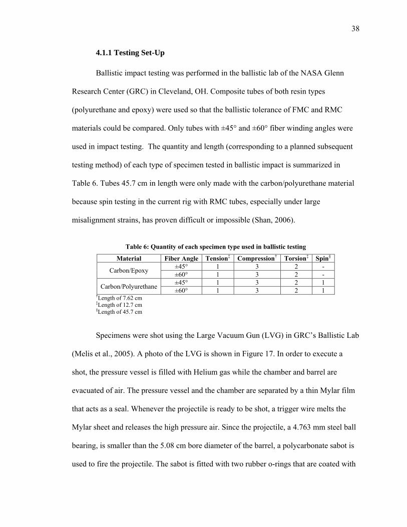
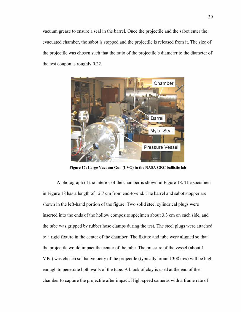
Specimens were shot using the Large Vacuum Gun (LVG) in GRClsquos Ballistic Lab
(Melis et al 2005) A photo of the LVG is shown in Figure 17 In order to execute a
shot the pressure vessel is filled with Helium gas while the chamber and barrel are
evacuated of air The pressure vessel and the chamber are separated by a thin Mylar film
that acts as a seal Whenever the projectile is ready to be shot a trigger wire melts the
Mylar sheet and releases the high pressure air Since the projectile a 4763 mm steel ball
bearing is smaller than the 508 cm bore diameter of the barrel a polycarbonate sabot is
used to fire the projectile The sabot is fitted with two rubber o-rings that are coated with
39
vacuum grease to ensure a seal in the barrel Once the projectile and the sabot enter the
evacuated chamber the sabot is stopped and the projectile is released from it The size of
the projectile was chosen such that the ratio of the projectilelsquos diameter to the diameter of
the test coupon is roughly 022
Figure 17 Large Vacuum Gun (LVG) in the NASA GRC ballistic lab
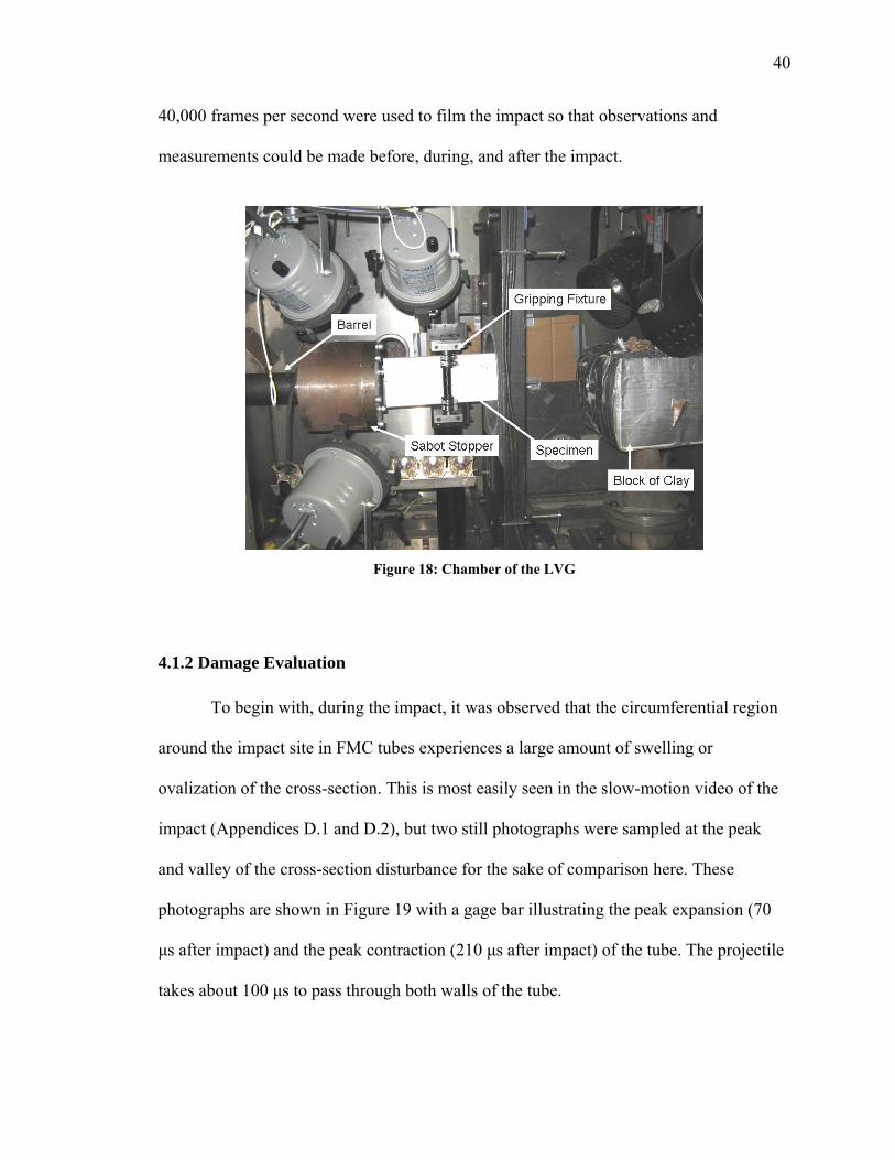
A photograph of the interior of the chamber is shown in Figure 18 The specimen
in Figure 18 has a length of 127 cm from end-to-end The barrel and sabot stopper are
shown in the left-hand portion of the figure Two solid steel cylindrical plugs were
inserted into the ends of the hollow composite specimen about 33 cm on each side and
the tube was gripped by rubber hose clamps during the test The steel plugs were attached
to a rigid fixture in the center of the chamber The fixture and tube were aligned so that
the projectile would impact the center of the tube The pressure of the vessel (about 1
MPa) was chosen so that velocity of the projectile (typically around 308 ms) will be high
enough to penetrate both walls of the tube A block of clay is used at the end of the
chamber to capture the projectile after impact High-speed cameras with a frame rate of
40
40000 frames per second were used to film the impact so that observations and
measurements could be made before during and after the impact
Figure 18 Chamber of the LVG
412 Damage Evaluation
To begin with during the impact it was observed that the circumferential region
around the impact site in FMC tubes experiences a large amount of swelling or
ovalization of the cross-section This is most easily seen in the slow-motion video of the
impact (Appendices D1 and D2) but two still photographs were sampled at the peak
and valley of the cross-section disturbance for the sake of comparison here These
photographs are shown in Figure 19 with a gage bar illustrating the peak expansion (70
μs after impact) and the peak contraction (210 μs after impact) of the tube The projectile
takes about 100 μs to pass through both walls of the tube
41
Figure 19 FMC tube swelling (left) and contracting (right) after impact plusmn45deg
Swelling or ovalization deformation of the RMC tubes under impact is not noticed
in the slow-motion videos (Appendix D3) This difference could suggest that the FMC
absorbs more energy during impact although drawing a definite conclusion from
deformation information alone is difficult because the tubes have different stiffnesses A
quantifiable calculation can be made to determine just how much energy is absorbed in
the FMC and RMC tubes during impact This calculation is made by measuring the
velocities of the projectiles before and after they enter the FMC and RMC tubes The
measurement is done by counting the number of pixels the projectile travels in each
subsequent image captured by the camera and comparing it to the frame rate of the
camera Pixels are converted into a distance via a calibration image containing a rod with
a known length For this calculation the interval between each image was 25 μs and the
exposure time was 1 μs Energy is calculated by Equation 23 where m is the mass of the
projectile (0444 g) and v is the velocity of the projectile The energy absorbed in both
tube types is shown in Table 7 The velocity measurements were made for plusmn45deg 762 cm
long tubes of both resin types (one data point each)
42
2
2
1mvE (23)
Table 7 Pre and post impact velocities energies
Velocity (ms) Energy (J)
Tube Type Rigid Flexible Rigid Flexible
Pre 304 304 206 205
Post 228 152 115 51
Absorbed - - 91 154
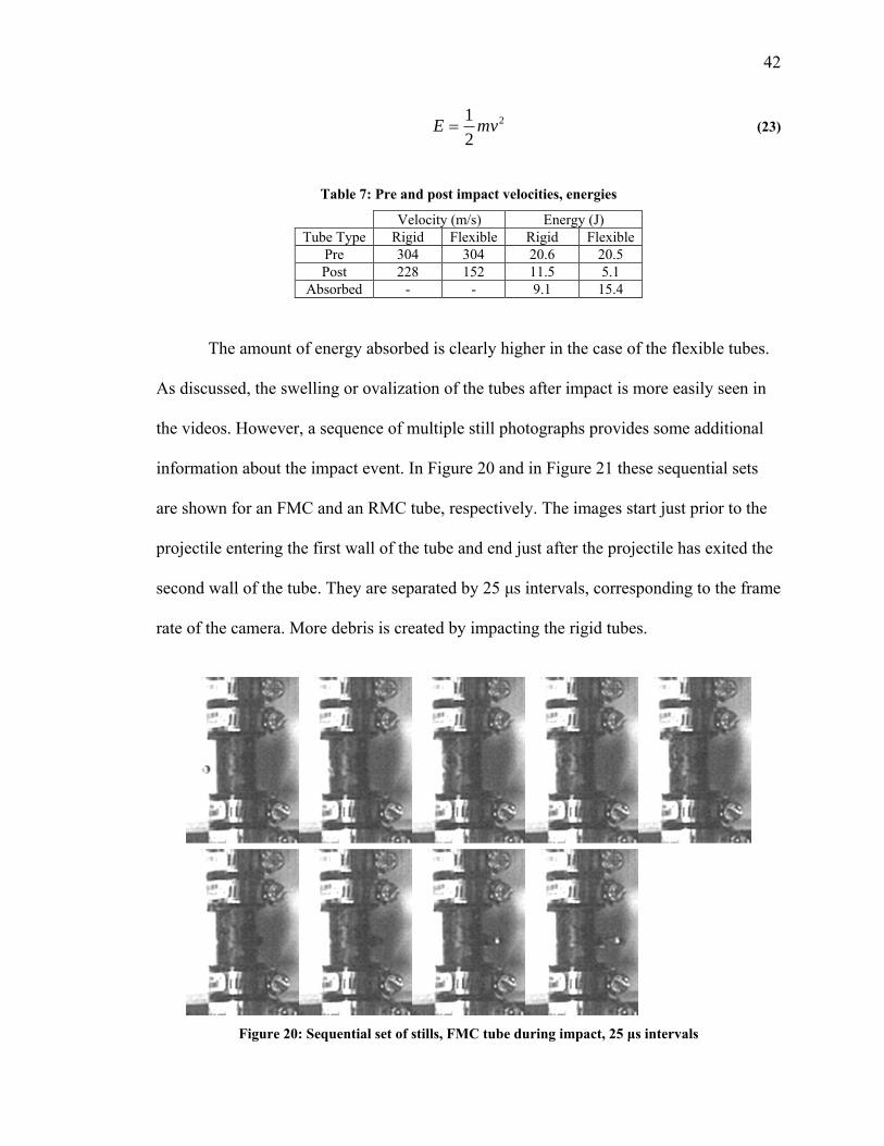
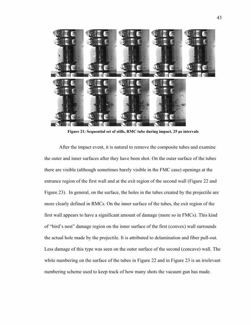
The amount of energy absorbed is clearly higher in the case of the flexible tubes
As discussed the swelling or ovalization of the tubes after impact is more easily seen in
the videos However a sequence of multiple still photographs provides some additional
information about the impact event In Figure 20 and in Figure 21 these sequential sets
are shown for an FMC and an RMC tube respectively The images start just prior to the
projectile entering the first wall of the tube and end just after the projectile has exited the
second wall of the tube They are separated by 25 μs intervals corresponding to the frame
rate of the camera More debris is created by impacting the rigid tubes
Figure 20 Sequential set of stills FMC tube during impact 25 μs intervals
43
Figure 21 Sequential set of stills RMC tube during impact 25 μs intervals
After the impact event it is natural to remove the composite tubes and examine
the outer and inner surfaces after they have been shot On the outer surface of the tubes
there are visible (although sometimes barely visible in the FMC case) openings at the
entrance region of the first wall and at the exit region of the second wall (Figure 22 and
Figure 23) In general on the surface the holes in the tubes created by the projectile are
more clearly defined in RMCs On the inner surface of the tubes the exit region of the
first wall appears to have a significant amount of damage (more so in FMCs) This kind
of ―birdlsquos nest damage region on the inner surface of the first (convex) wall surrounds
the actual hole made by the projectile It is attributed to delamination and fiber pull-out
Less damage of this type was seen on the outer surface of the second (concave) wall The
white numbering on the surface of the tubes in Figure 22 and in Figure 23 is an irrelevant
numbering scheme used to keep track of how many shots the vacuum gun has made
44
Figure 22 Visible damage in FMC tubes front view (left) and side view (right) plusmn60deg
Figure 23 Visible damage in RMC tubes front view (left) and side view (right) plusmn45deg
In addition to observing surface damage an invasive approach to detect damage
was explored Two FMC composite tubes (one plusmn45deg tube and one plusmn60deg) were used for X-
radiography After ballistic testing a photopenetrant is applied around the damaged
entrance and exit regions of the tube The penetrant solution is a dense low viscosity
fluid that contains 60 g of zinc iodide 10 mL of water 10 mL of isopropyl alcohol and
10 mL of Kodaklsquos ―Photo-Flo 200 The purpose of the penetrant is to migrate through
the cracks and delaminations of the composite The dense solution then shows up during
45
X-radiography where it penetrated the composite X-radiography pictures were taken
with an ICM X-ray emitter that was shot at the specimen with a phosphorous film that
was positioned behind the specimen The scanner SCANX12 ndash Portable the emitter and
film were made by All Pro Imaging and Air Techniques (Melville NY) The emitter was
placed 38 inches from the detector in order to achieve the best resolution possible The
emitter was set at 40 kV and the exposure time was anywhere from 25 ndash 35 seconds
The results of the X-radiography are shown in Figure 24 and in Figure 25 The hazy lines
in the photographs are micro cracks along the fiber winding angle whereas the dark
shaded areas are delaminations Although only one FMC tube of each angle type was
used in X-radiography it would seem that the region around the impact sites in FMC
tubes develops a substantial amount of matrix cracking all the way around the
circumference X-radiography was not performed on RMC tubes
Figure 24 X-radiography image of a flexible plusmn45deg tube after ballistic impact event
46
Figure 25 X-radiography image of a flexible plusmn60deg tube after ballistic impact event
4121 Spin Testing Damaged FMC Tubes
The details of the PSU spin rig and spin testing are described in detail in Section
62 but the results from spin testing a damaged FMC tube are given here for the sake of
thesis structure Only FMC tubes were tested in the spin rig because the robustness of the
rig will not accommodate RMC tubes (Shan 2006) Although the tubes see no torque in
this test the results will shed some light on how damaged shafts might perform in cyclic
fatigue The positioning of the bearings on the rig is such that they are meant to impose a
constant strain along the length of the tube For these tests plusmn45deg and plusmn60deg FMC tubes
with a length of 457 cm were used as described in Table 6 The lowest nominal strain
setting on the rig 025 was used and the rotational speed of 1200 rpm was selected A
254 cm clip gage extensometer is used to measure the actual strain at different positions
along the length of the tube This procedure is also described in more detail in Section
621 In the case of spin testing damaged tubes measuring the actual strain along the
length of the tube is particularly important because the damage region may be more
compliant than the rest of the tube Hence the misalignment from tip to end may be
47
concentrated in the damaged region while the rest of the tube sees less strain Measured
strains on the tensile and compressive sides of the tube are shown in Figure 26 At the
beginning of the spin test the mid span position at the site of the impact damage sees
about 026 strain while the other positions see about 020 strain
-03
-02
-01
0
01
02
03
Position Along Shaft
Str
ain
Compression Tension
Figure 26 Strain along damaged plusmn45deg flexible tube
After the strain is measured and recorded the motor is turned on and the
temperatures at different positions along the length are recorded by optical
thermocouples For this test the temperatures at the middle of the tube and at the quarter
span position closest to the motor were recorded The temperature and speed histories
versus time are shown in Figure 27 At first the temperature at the mid span position of
the tube seems like it may reach a steady state condition However at around 400
seconds the tube reaches an unstable condition The tube heats more at this location
because initially there is more strain at the mid span The heating causes the material to
be more compliant which in turn feeds more strain into that region The result is a
compounding effect that becomes unstable The peak in the temperature at the mid span
location corresponds to the point during the test where the tube essentially kinks When
Midspan Quarterspan
End of Tube End of Tube
48
this happens all of the misalignment from tip to end is concentrated in the kink
Consequently the tube cools at midspan and at quarterspan because the material in the
tube is no longer experiencing cyclic strain The tube is for all intensive purposes broken
It would no longer be able to carry a torsional load
0
200
400
600
800
1000
1200
1400
0 200 400 600 800 1000 1200
Time (s)
Sp
eed
(rp
m)
10
20
30
40
50
60
70
Tem
pera
ture
(degC
)
Speed
Mid Shaft T
Quarter Span T
Room T
Figure 27 Heating of damaged plusmn45deg flexible tube
After the misaligned spin test the photopenetrant solution was again applied to
the failed specimen so that another round of X-radiography photographs could be taken
to compare the damage from the impact and the damage from the spin test after impact
This comparison is shown in Figure 28 Clearly there is much more damage present after
the misaligned spin test All of the regions in the tube that were previously filled with
matrix cracking are now filled with large delaminations Similar undamaged tubes were
tested (mentioned in Section 62) in the spin rig under the same conditions These tubes
survived spin tests at twice the nominal strain and twice the speed without failing The
damage in the flexible tubes due to the ballistic impact event seems to have a noteworthy
effect for self-heating and cyclic fatigue The projectile causes damage which reduces the
stiffness of the tube in that localized region Due to the reduced stiffness more bending
FAILURE
49
strain is concentrated in that region resulting in more heating Higher temperatures also
reduce stiffness and a compounding effect seems to take place
Figure 28 X-radiography before (left) and after (right) misaligned spin test plusmn45deg FMC
Figure 29 X-radiography before (left) and after (right) misaligned spin test plusmn60deg FMC
42 Quasi-Static Testing
Axial tension and compression tests were carried out at two different places on
two different machines The first tension and compression tubular specimens of each type
listed in Table 6 along with their undamaged counterpart were tested in the
fatiguefracture lab Building 49 at the NASA Glenn Research Center The test machine
at GRC is a hydraulic axial-torsion machine The remaining tension and compression
tests for tubular specimens were performed at Penn State on a 267 kN screw-driven test
50
machine All torsion testing was performed at Penn State on a hydraulic axial-torsion
machine Quasi-static tension testing of the neat resin material was also performed on the
screw-driven test machine at Penn State
421 Tension and Compression
At NASA GRC load data were recorded by the load cell (222 kN range) in the
testing machine and strain was recorded by two pairs of cameras (two viewing the front
of the specimen and two viewing the back) These cameras take successive sets of
pictures during the test that are sent to a software program after the test where they are
compared to one another to make full-field strain measurements on both sides of the
specimen This technique is called digital image correlation and in this case is performed
by an optical deformation analysis software package called ARAMIS made by GOM
International AG (Widen Switzerland) The software can also pick two points in the field
of view and measure the relative displacement between them mimicking a strain
measurement by a clip gage For these tests longitudinal (254 cm) and transverse (127
cm) virtual clip gages were used For the case where tubes with ballistic damage were
being tested the damage regions were aligned with the front (entrance side) and back
(exit side) cameras and the virtual clip gage spanned the damage region Since the
surface of the composite is black and reflective ultra flat white and black spray paints are
used to create a speckle pattern on the surface of the composite This pattern and correct
lighting of the specimen allows for more accurate measurements by the ARAMIS
software when comparing two images
At Penn State load data were recorded by the load cell (267 kN range) while
strain data for tubular specimens was recorded by two 254 cm clip gage extensometers
51
located 180deg from each other Longitudinal strain data for the neat resin coupon was
recorded by a laser extensometer whereas transverse strain data was recorded by a 127
cm clip gage extensometer For the case where tubes with ballistic damage were being
tested an extensometer spanned the holes made by the projectile on either side Voltage
outputs from the extensometers and load cell were recorded by a data acquisition
computer running a LabVIEW program
An example of the gripping set-up used in tension testing of tubes is shown in
Figure 30 This photograph shows a composite tube with the black and white speckle
pattern bonded into a set of steel swivel grips that are held by the hydraulic-powered
grips on the testing machine at GRC The tension testing set-up for tubes would appear
much the same at Penn State except the testing machine grips at Penn State are
mechanical wedge grips For tension testing of tubes the specimens were first prepared
by wiping down the inside and outside of the tube with a cloth wet with acetone This
removes any dust and silicon release that is left over from fabrication The tube
specimens were then bonded into a set of grips using a bonding adhesive The adhesive
used with the carbonepoxy system is called Loctite Weld made by Henkel Corporation
(Avon OH) The adhesive used with the carbonpolyurethane system is called Devcon
Plastic Weldertrade made by ITW Devcon (Danvers MA) The swivel grips are further
illustrated in Figure 31 They can be taken apart and have a set of swivel bearings to
eliminate spurious moments during testing After the binding adhesive is applied the
specimen and the grips are placed in an oven at 60degC for at least 6 hours to allow the
adhesive to cure When the test is complete the specimen is cut out of the grips and the
steel inner and outer sleeves are placed in a burnout oven at 510degC for approximately 30
minutes Once the sleeves have cooled down to room temperature they are taken apart
52
sanded down with grit cloth and wiped clean with a cloth wetted with acetone They are
then re-assembled for future testing The rectangular coupon of neat resin is simply
gripped by mechanical wedge grips in tension testing
Figure 30 Quasi-static tension testing gripping set-up and tubular specimen with speckle pattern
Figure 31 Schematic of grip used in quasi-static tension testing (Shan 2006)
Steel swivel grips
53
An example of the gripping set-up used in compression testing is shown in Figure
32 This photograph shows a composite tube potted into grooves in a pair of disk-shaped
steel end fixtures These end fixtures serve as platens that are compressed by the load
frame of the testing machine at Penn State The hemispherical joint shown at the bottom
of the photograph was used to eliminate the possibility of moments being introduced due
to misalignment of the load train The compression testing set-up would appear much the
same at GRC For compression testing the disk-shaped steel end fixtures are heated to
about 80degC on a hot plate As the fixtures heat a fusible alloy contained within the
grooves of the fixtures melts The commercial name of the alloy in this case is
Cerrobend Melting of the alloy allows the composite tubes to fit into the grooves of the
end fixtures Once the tube was fitted into the groove the fixture and the tube were
removed from the hot plate and allowed to cool When the alloy cools it also expands
which clasps the composite tube tightly and helps prevent end-brooming during
compression testing When a test is complete the end fixtures are heated again the alloy
melts the test specimens are removed from the fixtures and the fixtures are ready to be
used again
54
Figure 32 Quasi-static compression testing gripping set-up
The testing set-up for tension testing the neat resin material is shown in Figure 33
A laser extensometer was used to measure longitudinal strain because of the high
compliance of the polymer being tested The laser extensometer works by placing two
reflective strips onto the specimen that reflect light back to the extensometer From the
incident angle of the reflected light the laser extensometer can calculate how far apart the
reflective strips are positioned from one another This initial distance was recorded as the
gage length (about 38 cm in this case) The sensitivity of the laser was set to the highest
with 5 V = 01 inches The width of the specimens was selected carefully to
accommodate the 127 cm clip gage The clip gage was calibrated and affixed to the
specimen with a set of rubber bands The distance between the mechanical wedge grips
was about 8 cm
Grooves End Fixtures
Hemispherical
Joint
55
Figure 33 Neat resin testing set-up
For the axial tension and compression tests stress is calculated by dividing the
load by the cross sectional area of the tubes The geometric properties of each of the
tubes are tabulated in Table 2 and in Table 3 and the geometric properties of the neat
resin coupon are tabulated in Table 5 For tests where clip gage extensometers were used
to measure deformation strain is calculated by transforming the voltage data into
displacement by the equation determined during calibration For the laser extensometer
the strain is calculated by converting voltage data into displacement by the conversion
equation mentioned above Axial strain rates for tension and compression testing of tubes
were typically about 150 μεs whereas for the neat resin the strain rate was about 220
μεs
422 Torsion
Torsion tests were carried out at Penn State on a hydraulic axial-torsion load
frame The load frame was set to angle control for the torsional actuator and force control
for the axial actuator The actuator rotates 10 degrees in 10 minutes throughout the length
of the test which corresponds to a shear strain rate of about 33 μγs for the 988-mm-long
gage section of the test specimen For these pure torsion tests the axial actuator was set at
56
a force value of zero The feedback mechanism for angle control is the rotary variable
differential transformer (RVDT) The feedback mechanism for force control is the load
cell in the testing machine Because the angular displacement measured by the RVDT is
the displacement of the actuator some assumptions must be made as to how much
angular displacement the composite tube is actually experiencing The assumptions made
here are that the steel end grips (Figure 34) are torsionally rigid and that the tube is
rigidly bonded into these grips That is the length of the exposed composite tube (988
cm) and the angular displacement of the crosshead are used to calculate shear strain
These assumptions may introduce some inaccuracies The adhesive material used to bond
the tube into the grips certainly has some compliance The bonding adhesives used in
torsion testing are the same that were used in tension testing (mentioned in Section 421)
After testing the tubes were burned out of the grips and the grips were cleaned
and prepared for another test in the same manner as for the tension grips Shear stress ηxy
at the outer surface of the tube is calculated by
l
rGG
J
Trxyxyxyxy
00 (24)
where T is the torque on the tube r0 is the outermost radius of the tube and J is the polar
moment of inertia for a round tube For a circular hollow tube J is given by
)(2
44
io rrJ
(25)
where ri is the inner radius of the tube The calculation for shear strain can also be seen in
Equation 24 where θ is the angle of twist and l is the gage length of the test specimen
57
Figure 34 Steel end grips used in torsion testing
43 Quasi-Static Test Results
Stress-strain curves were generated in tension compression and torsion testing
for damaged and undamaged tubes Values of Younglsquos modulus and ultimate strength
were determined from these curves and are tabulated here In a few cases where
transverse strains were measured the Poissonlsquos ratios were also determined Generally
speaking the test matrix for damaged specimens follows the outline shown in Table 6
although not all of the tests represented in Table 6 were completed successfully due to
some laboratory mishaps The test matrix for undamaged specimens is shown in Table 8
Observations about how the specimens deformed during testing and their failure modes
as well as the results from testing the neat resin in quasi-static tension are covered here
Table 8 Test matrix for undamaged composite tubes
Material Winding Angle Tension Compression Torsion Spin Testing
CarbonPolyurethane plusmn20deg plusmn30deg plusmn45deg plusmn60deg plusmn832 3 3 11 12
CarbonEpoxy plusmn45deg plusmn60deg 1 3 1 - 1plusmn45deg and plusmn60deg tubes only 2plusmn30deg plusmn45deg and plusmn60deg tubes
For testing performed at GRC the information from the longitudinal and
transverse virtual clip gages generated stress-strain curves and plots of negative
transverse strain versus longitudinal strain A snapshot during one of these tests is shown
58
in Figure 35 with the color mapping scheme (generated after testing by the software
program) overlaid onto an image of the specimen The strain in the longitudinal loading
direction of the tube (vertical in this picture) is represented by εx and the red crosses
indicate the end points of the virtual clip gages A video of a damaged plusmn45deg FMC tube in
tension is shown in Appendix D4 For testing performed at Penn State only longitudinal
mechanical clip gages were used so only stress-strain curves were generated The stress-
strain curves from the front and back of the tubes were averaged in case there was any
bending of the tube during the test A sample stress-strain curve for one of the specimens
tested at GRC is shown in Figure 36
Figure 35 Snapshot a rigid undamaged plusmn45deg tube in tension
εx
59
0
20
40
60
80
100
120
140
160
0 001 002 003 004 005 006 007 008
Strain εx (mm)
Str
ess
σ
x (M
Pa)
Figure 36 Representative average tensile stress-strain data generated by a virtual 254 cm clip gage ndash
rigid undamaged plusmn45deg tube
A sample plot of negative transverse strain versus longitudinal strain and a sample
measurement (typically in the longitudinal strain range of about 1) of the Poissonlsquos
ratio of one of the composite tubes are shown in Figure 37 Longitudinal and transverse
strain measurements from the front and back of the tube were averaged and a straight line
was fit to the plot to determine the structural Poissonlsquos ratio νxy All of the Poissonlsquos ratio
measurements are summarized later in this section
R2 = 09973
0000
0002
0004
0006
0008
0010
0012
0 0002 0004 0006 0008 001 0012
Longitudinal Strain ε x (mm)
Neg
ati
ve T
ran
svers
e S
train
-ε
y (
mm
)
Figure 37 Representative measurement of Poissonrsquos ratio ndash flexible undamaged plusmn45deg tube in
tension
νxy = 0884
60
A comparison of longitudinal stress-strain curves from each testing set-up for
flexible undamaged plusmn45deg tubes tested in tension is shown in Figure 38 This graph
shows the strain region where the modulus measurement is made The modulus is taken
as a secant modulus calculated in the range of 0 ndash 600 με for all tests (εx in tension and
compression and γxy in torsion) A linear fit to the data in this region is used to make the
measurement because of data noise issues Although this seems to be appropriate because
typical R2 values for the linear fit are higher than 095 for tests run at GRC and Penn
State Also beyond this strain range the elastic response becomes noticeably nonlinear
especially for the axial tension and compression tests For example from the data shown
from the DIC in Figure 38 the modulus measured in the 0 ndash 600 με range is 409 GPa
while the modulus measured in the 0 ndash 3000 με range is 255 GPa ndash almost a 38
reduction Operational strain ranges for εx are expected to be less than 2000 με All of the
modulus and ultimate strength values are summarized later in this section
0
2
4
6
8
10
12
14
0000 0001 0002 0003 0004 0005
Strain (mm)
Str
ess
(M
Pa)
DIC (GRC)
Clip Gage (Penn State)
Figure 38 Strain measurement comparison DIC (GRC) and clip gage (Penn State) a flexible
undamaged plusmn45deg tube in tension
Region of modulus
measurement
61
In tension and compression testing the full-field strain measurement at GRC
allows for observations to be made about deformation patterns that arise on the entire
surface of the tube during loading This information is not captured with a simple clip
gage and it provides insight into the evolution of damage in impacted and non-impacted
composite tubes Due to the size of the field of view of the cameras the entire specimen
could not be photographed during testing The area of the full-field strain measurement
and the positioning of the clip gage for a damaged tube in tension are shown in Figure 39
The configuration for tubes in compression and undamaged tubes is very similar
Sequential photographs with longitudinal strain overlay of tubes being loaded are shown
in Figures 40 ndash 42 These photographs simply show the development of damage during
loading and are not sampled at similar rates from one test to another These images show
the front side (projectile entrance) of the tubes In both FMC and RMC tubes regions of
high strain seem to accumulate in patterns that resemble the tow pattern in which the tube
was fabricated The regions of highest strain in the undamaged tubes appear to follow the
last or next to last tow that was wound onto the part Also in undamaged tubes strain is
distributed throughout the entire tube whereas in damaged tubes material deformation
seems to be concentrated in the damage region Because of this localized material
deformation the modulus measurements mentioned later in this section are really a
smeared stiffness over the gage length of the extensometer Modeling reductions in
stiffness and strength may require a more in-depth analysis When comparing the tensile
behavior of the RMC tubes and FMC tubes it appears that the damage region in the
RMC is fairly localized and in the FMC it is more spread out Similar material
deformation and failure behavior is observed in tension and compression Failure in the
form of matrix cracking and fiber shearing occurs in a spiral pattern oriented along the
62
fiber winding angle For damaged tubes this spiral pattern intersects the boundary of the
hole made by the projectile
Figure 39 Schematic of full-field strain measurement and slip gage positioning for a tube in tension
Figure 40 Snapshots of longitudinal strain in rigid plusmn45deg undamaged (top) and damaged (bottom)
tubes tested in tension with stress-strain curves from digital clip gage
ζx
(MP
a)
εx ()
160
0
ζx
(MP
a)
0
0
εx () 8
8
εx 160
0
63
Figure 41 Snapshots of longitudinal strain in flexible plusmn45deg undamaged (top) and damaged (bottom)
tubes tested in tension with stress-strain curves from digital clip gage
Figure 42 Snapshots of longitudinal strain in flexible plusmn45deg undamaged (top) and damaged (bottom)
tubes in compression with stress-strain curves from digital clip gage
Figure 43 is provided in order to further illustrate the difference in the damage
regions of FMC and RMC tubes All of the tubes in Figure 43 are experiencing the same
remote axial strain 2000 με which is a typical maximum value that an FMC tube might
- ζ
x (M
Pa)
εx ()
35
0
- ζ
x (M
Pa)
35
0
0
εx () 8
8
ζx
(MP
a)
εx ()
35
0
ζx
(MP
a)
35
0
0
εx () 8
8
εx
εx
64
experience in service The damage in the FMC tube seems to be more spread out while
the damage in the rigid tube appears to be more localized This is consistent with the
more extensive ―birdlsquos nest damage seen on the inner surface of the FMC tubes in
comparison to the RMC tubes
Figure 43 Full-field strain measurement under tensile loading FMC and RMC all plusmn45deg front side
Failure in torsion testing occurred in one of two ways The failure region during
loading was either concentrated at the site where the impact was made (a crushing mode)
or matrix cracking and fiber shearing occurred in a spiral pattern much the same way as it
did in tension and compression testing The crushing mode was only seen in damaged
tubes although not all damaged tubes saw this mode of failure Some damaged tubes
failed with the spiral pattern intersecting the hole from the projectile at its boundary
These two types of failure modes are shown in Figure 44
Load
ing D
irec
tion
65
Figure 44 Failure modes in torsion crushing in a plusmn45deg FMC (left) and spiral pattern in a plusmn60deg
(right)
All modulus and ultimate strength measurements in tension compression and
torsion of filament-wound carbonpolyurethane and carbonepoxy composite tubes with
varying fiber winding angles are shown in Tables 9 ndash 14 where Cv is the coefficient of
variation For the most part coefficients of variation were less than 15 for undamaged
tubes and considerably larger for damaged tubes Results matched well for tension and
compression testing across testing platforms
Table 9 Quasi-static moduli in axial tension
FMC RMC
Fiber Angle Modulus (GPa) Average Modulus (GPa) Cv () Modulus (GPa)
Undamaged
plusmn20deg 311
322 - -
334 -
plusmn30deg
116
107 12
-
113 -
925 -
plusmn45deg
4091
390 9
1701
419
391
plusmn60deg 1861
246 25
1041
255 -
298 -
plusmn832deg 145
171 - -
197 -
Damaged plusmn45deg 2951 - - 1161
plusmn60deg 2031 2 - - -
1Tested at NASA GRC
2Data is suspect ndash order of magnitude differences in strain measurement on front and back of specimen
66
Table 10 Quasi-static moduli in axial compression
FMC RMC
Fiber Angle Modulus
(GPa)
Average
Modulus
(GPa)
Cv () Modulus
(GPa)
Average
Modulus
(GPa)
Cv ()
Undamaged
plusmn20deg
224
254 10
-
- - 273 -
264 -
plusmn30deg
109
983 10
-
- - 960 -
898 -
plusmn45deg
4281
401 6
1511
154 - 395 157
380 -
plusmn60deg 2061
262 26
1021
101 - 241 103
338 975
plusmn832deg 164
157 7 -
- - 149 -
Damaged
plusmn45deg
1641
273 40
9881
106 - 274 114
381 -
plusmn60deg
1081
120 17
4371
584 22 144 645
110 670
1Tested at NASA GRC
Table 11 Quasi-static moduli in torsion
Shear Modulus (GPa)
Fiber Angle FMC RMC
Undamaged plusmn45deg 187 218
plusmn60deg 162 206
Damaged plusmn45deg 945 210
plusmn60deg 780 150
67
Table 12 Quasi-static ultimate strength in axial tension
FMC RMC
Fiber Angle Strength (MPa) Average Strength (MPa) Cv () Strength (MPa)
Undamaged
plusmn20deg -
- - -
- -
plusmn30deg
701
706 5
-
677 -
74 -
plusmn45deg
2971
296 1
13721
297 -
295 -
plusmn60deg 2151
249 13
6471
252 -
281 -
plusmn832deg 100
101 - -
102 -
Damaged plusmn45deg 1531 - - 8711
plusmn60deg 1141 - - 3631
1Tested at NASA GRC
Table 13 Quasi-static ultimate strength in axial compression
FMC RMC
Fiber Angle Strength
(MPa)
Average
Strength
(MPa)
Cv () Strength
(MPa)
Average
Strength
(MPa)
Cv ()
Undamaged
plusmn20deg
821
765 7
-
- - 725 -
75 -
plusmn30deg
507
501 4
-
- - 48 -
517 -
plusmn45deg
3281
369 11
1341
139 - 408 145
37 -
plusmn60deg 3221
362 10
1451
145 1 366 144
397 145
plusmn832deg
315
275 23
-
- - 308 -
203 -
Damaged
plusmn45deg
1761
206 20
8511
837 2 188 822
253 -
plusmn60deg
1391
154 10
4281
529 21 153 511
169 648
1Tested at NASA GRC
68
Table 14 Quasi-static strength in torsion for ballistic tolerance comparison
Torsional Strength (MPa)
Fiber Angle FMC RMC
Undamaged plusmn45deg 672 -
plusmn60deg 638 555
Damaged plusmn45deg 621 503
plusmn60deg 677 253
The measurements of the Poissonlsquos ratios νxy of the composite tubes that were
obtained are shown in Table 15 Poissonlsquos ratio measurements were only made for
undamaged tubes
Table 15 Poissonrsquos ratios of the composite tubes tested at Glenn
FMC RMC
Fiber Angle Tension Compression Tension Compression
plusmn45deg 088 100 062 dagger
plusmn60deg 060 050 dagger 031
daggerBad transverse strain measurement
A graph of the transverse and longitudinal strains used to make the Poissonlsquos ratio
measurement of the neat resin is shown in Figure 45 The Poissonlsquos ratio for the
LF750DDC31 DA neat resin is 038 The secant modulus (0 ndash 1000 με) is 310 MPa
00
05
10
15
20
25
30
35
40
0 1 2 3 4
Longitudinal Strain ()
- T
ran
sver
se S
trai
n (
)
Figure 45 Poissons ratio measurement for LF750DDC31 DA neat resin
69
In order to illustrate the differences in the moduli and strengths of damaged and
undamaged FMC and RMC tubes normalized bar charts are shown in Figures 46 ndash 49 A
knockdown is the amount of reduction in a material property (modulus or strength) due to
ballistic impact For knockdowns in modulus in tension and compression considering
certain fiber angles the FMC may perform better than the RMC or vice versa But for the
most part there is no significant difference between the knockdowns in moduli for FMC
and RMC materials in tension and compression In torsion however the knockdowns in
modulus for the FMC case (~50) seem to be clearly higher than the RMC case (~20)
For knockdowns in strength in tension and compression the findings are very similar to
knockdowns in modulus While considering certain fiber angles the FMC may perform
better than the RMC or vice versa But for the most part there is no significant difference
between the knockdowns in strength for FMC and RMC materials in tension and
compression In torsion however the knockdowns in strength for the FMC case are
almost 90 while the knockdowns in strength for the RMC case are about 55
0
20
40
60
80
100
120
Tension Compression Torsion
Type of Test
No
rmali
zed
Mo
du
lus
()
Undamaged
Damaged plusmn45deg
Damaged plusmn60deg
Figure 46 Moduli before and after ballistic damage FMC
Data is suspect ndash strain measurement discrepancy
70
0
20
40
60
80
100
120
Tension Compression Torsion
Type of Test
No
rmali
zed
Mo
du
lus
()
Undamaged
Damaged plusmn45deg
Damaged plusmn60deg
Figure 47 Moduli before and after ballistic damage RMC
0
20
40
60
80
100
120
Tension Compression Torsion
Type of Test
No
rmali
zed
Str
en
gth
(
)
Undamaged
Damaged 45
Damaged 60
Figure 48 Ultimate strengths before and after ballistic damage FMC
71
0
20
40
60
80
100
120
Tension Compression Torsion
Type of Test
No
rmali
zed
Str
en
gth
(
)
Undamaged
Damaged 45
Damaged 60
Figure 49 Ultimate strengths before and after ballistic damage RMC
45 Determination of Ply Elastic Properties
The determination of the material properties for the LF750D composite is a
research objective and is made here Ply elastic properties were only determined for the
flexible matrix composite material Each ply in a laminated composite can be modeled as
an orthotropic material These orthotropic materials have four independent material
properties that fully characterize the ply namely E1 E2 v12 and G12 The 1-2 coordinate
system is defined in Figure 50 which shows a section of a ply where the 1-direction is
coincident with the fiber direction The x-y coordinate system is the structural coordinate
system of the composite part with the x-axis the direction of applied loading When these
plies are stacked up into a laminate the four ply elastic properties are then able to predict
the structural response of the laminate through classical laminated plate theory (CLPT ndash
Daniel and Ishai 2006)
72
Figure 50 Schematic of ply angle θ
Material properties of the carbonpolyurethane composite were obtained through a
few different ways The major in-plane Poissonlsquos ratio was determined by rule of
mixtures That is
mfaffa VV )1(12 (26)
where Vfa is the fiber volume fraction (assumed to be 059 ndash an average from the values
of the 20 mm tubes in Table 3) νf is the Poissonlsquos ratio of the fiber (assumed to be 028 ndash
Krucinska and Stypka 1991) and νm is the Poissonlsquos ratio of the polyurethane matrix
material measured as 038 The value of ν12 for the FMC was determined to be 033 The
minor Younglsquos modulus E2 was determined by testing undamaged hoopwound tubes in
tension and compression Although the actual winding angle for these tubes is 832deg the
moduli measured from these tests are assumed to be E2 According to classical laminated
plate theory (using the values in Table 16) the difference between the axial modulus for
an 832deg tube and a 90deg tube is less than 125 The values of the minor Younglsquos
modulus in tension and compression were determined to be 171 GPa and 157 GPa
73
respectively The in-plane shear modulus was determined by the [plusmn45]ns coupon test
(Daniel and Ishai 2006) In this case the coupon was an undamaged angle-ply tube of
the 20 mm inner diameter type Longitudinal and transverse strains were measured in
these kinds of tests (using the testing machine at NASA GRC) and were transformed into
shear strains in the principal coordinate system Longitudinal stress was also transformed
into shear stress in the principal coordinate system If in the linear range of stress and
strain the in-plane shear modulus can be calculated by
)1(2)(212
1212
xy
x
yx
x EG
(27)
where 12 is the in-plane shear stress 12 is the in-plane shear strain x is the
longitudinal stress x is the longitudinal strain y is the transverse strain xE is the
longitudinal or axial modulus xy is the Poissonlsquos ratio obtained from the initial slopes
of the curves of the plusmn45deg tube (Daniel and Ishai 2006) The longitudinal moduli and
Poissonlsquos ratios are used to calculate G12 These values and their respective strain ranges
of calculation are given in Section 43 The tension and compression tests at GRC yield
values of 109 and 107 GPa for the in-plane shear moduli of the FMC respectively
The determination of the major Younglsquos modulus is not a trivial task First the
rule of mixtures was used to calculate E1 but this value appeared to be much too large
when comparing CLPT theory (with the three previously mentioned ply elastic
properties) and experimental data on the Ex versus fiber winding angle (θ) curve ndash Figure
51 So since the value of E1 has only a major influence on lower fiber angles it was
adjusted manually so that the curve generated by CLPT would fit best to the tensile ndash
CLPT (T) compressive ndash CLPT (C) and average of tensile and compressive moduli ndash
74
CLPT (Avg) for the plusmn20deg tube These three curves generated by three values of E1 are
shown with experimental data with scatter bars in Figure 51 An expanded view of the
same graph for higher fiber angles is shown in Figure 52 The ply elastic material
properties used along with CLPT to generate curves are tabulated in Table 16
0
10
20
30
40
50
60
70
0 10 20 30 40 50 60 70 80 90Fiber Angle (deg)
Axia
l M
odulu
s E
x (
GP
a)
Tension
Compression
CLPT (T)
CLPT (C)
CLPT (Avg)
Figure 51 FMC Ex vs θ experiments and theory CLPT (T C and Avg)
00
05
10
15
20
25
30
35
40
45
50
40 45 50 55 60 65 70 75 80 85 90
Fiber Angle (deg)
Ax
ial
Mo
du
lus
Ex (
GP
a)
Tension
Compression
CLPT (T)
CLPT (C)
CLPT (Avg)
Figure 52 FMC Ex vs θ experiments and theory CLPT (T C and Avg) reduced range
75
Table 16 Ply elastic material properties for fitting routine to tension and compression testing
Parameter Values
CLPT (T) CLPT (C) CLPT (Avg)
E1 (GPa) 690 430 510
E2 (GPa) 171 157 164
G12 (GPa) 109 107 109
ν12 033 033 033
The fitting line CLPT (Avg) in Figure 51 and in Figure 52 fits well to within less
than 3 for all tube angles except for plusmn30deg where it over predicts by 24 and for plusmn60deg
where it under predicts by 13 An interesting observation to make is on how well these
ply elastic properties predict the structural shear modulus Gxy of the undamaged 20 mm
plusmn45deg tubes in torsion testing As it turns out the value of E1 in Table 16 is much too low
to accurately predict Gxy of the plusmn45deg tube So another method was used to choose
appropriate ply elastic properties that would predict shear moduli well The values of E2
G12 and ν12 that were determined from the average fitting routine mentioned above were
fixed while E1 was allowed to vary so that a best fitting curve of Gxy versus θ generated
by CLPT could be found The value of E1 was allowed to vary because the other three ply
elastic properties do not have a major influence on the Gxy curve near plusmn45deg That best fit
curve denoted by CLPT (Torsion) is shown in Figure 53 and the ply elastic properties are
tabulated in Table 17
76
0
5
10
15
20
25
0 15 30 45 60 75 90
Fiber Angle (deg)
Sh
ear
Mo
du
lus
Gxy
(G
Pa) Torsion
CLPT (Torsion)
Figure 53 Gxy vs θ experiments and theory CLPT (Torsion)
Table 17 Ply elastic material properties for fitting routine to torsion testing
Parameter Values
CLPT (Torsion)
E1 (GPa) 790
E2 (GPa) 164
G12 (GPa) 109
ν12 033
The fitting line in Figure 53 agrees well with the limited experimental data with
deviations of 7 However the value of E1 for CLPT (Torsion) is considerably higher
than the value of E1 for CLPT (Avg) For comparison the value of E1 that is chosen to fit
to the Gxy experimental data is used to generate an Ex versus θ curve This is shown in
Figure 54 with an expanded view of the same graph for higher fiber winding angles
shown in Figure 55
77
0
10
20
30
40
50
60
70
80
0 10 20 30 40 50 60 70 80 90
Fiber Angle (deg)
Mo
du
lus
(GP
a)
Tension
Compression
CLPT (Avg)
CLPT (Torsion)
Figure 54 Ex vs θ experiments and theory CLPT (Avg and Torsion)
00
05
10
15
20
25
30
35
40
45
50
40 50 60 70 80 90
Fiber Angle (deg)
Mo
du
lus
(GP
a)
Tension
Compression
CLPT (Avg)
CLPT (Torsion)
Figure 55 Ex vs θ experiments and theory CLPT (Avg and Torsion) reduced range
While CLPT (Avg and Torsion) fit the experimental data well for winding angles
greater than 45deg there are some major discrepancies for lower fiber winding angles For
plusmn30deg CLPT (Avg) over predicts by 24 while CLPT (Torsion) over predicts by 41 For
plusmn20deg CLPT (Avg) is right on the average of the tensile and compressive data points while
CLPT (Torsion) over predicts by 34 As another point of reference the value of E1
predicted by the rule-of-mixtures for Vfa = 059 Ef = 245 GPa (Younglsquos modulus of the
78
fiber ndash Hexcel 2009) and Em = 310 MPa (Younglsquos modulus of the neat resin) is 145
GPa If a unidirectional 0deg tube were to be tested in axial tension it is believed that the
modulus would be close to the value calculated by the rule-of-mixtures For these
reasons a value of E1 = 79 GPa is considered to be the major in-plane Younglsquos modulus
of the FMC
46 Summary
The results from the ballistic impact testing seem to show that more damage was
created in the FMC tubes than in the RMC tubes from the steel ball bearing projectile
Most evidence from the initial inspection after impact to the swelling observed during
impact to the amount of energy absorbed by the two different tubes to the full-field
strain measurements made by the DIC show that the damage region in the FMC was
larger and more widespread A comparison between FMC and RMC tubes was not made
using X-radiography but this technique showed extensive matrix cracking in the
circumferential region around the impact site in FMC tubes The swelling of the tube and
the considerably (~50) larger amount of energy that the FMCs absorbed during impact
can be explained by the high strain to failure of elastomeric materials The matrix
material deforms much more in the FMCs during impact absorbs more energy resulting
in what seems to be overall more material fracture The matrix material in the RMC is
rigid and has a low strain to failure In this case the projectile fractures the material at the
impact site makes a clearly defined hole and does not seem to propagate damage as
extensively beyond the impact site Again only FMC tubes were used in spin testing
because RMC tubes were too stiff to be misaligned in the spin rig However during spin
testing of damaged FMC tubes a compounding effect of localized strain and heat was
79
observed at the impact site where the tube eventually kinked and failed Similar
undamaged tubes were also tested (mentioned in Section 62) that survived tests at twice
the nominal strain and twice the speed Interestingly enough the knockdowns in the
tensile and compressive quasi-static modulus and strength for FMCs and RMCs were
comparable For some fiber angles one material seemed to perform better than the other
but across the board there was no material that seemed to outperform the other in
modulus and strength knockdowns in tension and compression
In torsion while RMCs saw about a 20 knockdown in shear modulus FMCs
saw about a 50 knockdown In terms of ultimate strength RMCs saw about a 55
knockdown where FMCs saw about a 90 knockdown An interesting result of torsion
testing is that no tubes failed by torsional buckling Either the spiral pattern of sheared or
buckled fibers at a local level or the crushing of damaged material at the impact site was
seen as failure modes This contrasts to the results seen by Bauchau et al (1988) and
may be due to the differences in geometries of the test specimens In torsion testing of the
plusmn45deg and plusmn60deg tubes the fibers are primarily loaded In tension and compression testing
of the same angles the matrix tends to be the primary constituent that is loaded For this
reason the large knockdowns in torsional modulus and strength in FMC tubes may be
attributed to the larger regions of fiber pull-out seen on the inside of impacted tubes
Quasi-static testing was carried out in tension compression and torsion on two
different load frames Results agreed well across testing platforms Where applicable
coefficients of variation for undamaged tubes were less than 15 for quasi-static
modulus and strength measurements (with a few minor exceptions) The variation among
damaged tubes was considerably more
80
It is clear that conventional laminated plate theory does not accurately predict the
axial and torsional stiffnesses of angle-ply FMC tubes First of all the differences in the
tensile and compressive axial moduli for the same fiber winding angle can be anywhere
from 3 ndash 27 different In general a larger discrepancy is seen between tension and
compression for lower winding angles While appropriate values for E2 G12 and ν12
coupled with laminated plate theory may predict the axial moduli of higher angled tubes
(above plusmn45deg) laminated plate theory fails when predicting axial moduli of tubes with
winding angles close to 0deg and torsional moduli of tubes with winding angles close to
45deg The common denominator between these two scenarios is the majority of the load is
applied in the fiber direction Perhaps the fact that the fibers in these composites are
woven in an undulated manner and surrounded by a soft flexible matrix is the reason
why there is such a discrepancy between CLPT and experiments The composites in the
current investigation do not have stacked discrete composite plies comprised of stiff
fibers surrounded by a stiff matrix ndash the situation upon which classical laminated plate
theory was developed
The values of E1 shown in Tables 16 ndash 17 (51 and 79 GPa) are significantly less
than the value of E1 calculated by rule of mixtures (145 GPa) If tensile and compressive
axial moduli of angle-ply tubes were measured for fiber winding angles less than 20deg it
is believed that the value of E1 to accurately predict the moduli of these tubes would
increase (from 51 GPa for a plusmn20deg tube) So perhaps a modified version of laminated plate
theory with a major in-plane Younglsquos modulus that is dependent on the fiber winding
angle would accurately predict the structural response of angle-ply FMC tubes for all
fiber winding angles Developing a modified version of classic lamination theory to
predict the axial and torsional stiffnesses of FMC tubes is beyond the scope of the current
81
work although a previous attempt effects to model axial stiffness of FMC tubes
considering fiber undulation has been made with moderate success (Zindel 2009)
82
Chapter 5 Determination of Viscoelastic Lamina Properties
The viscoelastic material properties in the transverse and shear directions of a
composite lamina are sensitive to temperature and frequency Because these properties
are used over varying temperature and frequency ranges to calculate the steady state
temperature in misaligned spinning composite shafts it is necessary to model these
variations accurately The approach for modeling and the experimental determination of
these properties for the carbonpolyurethane composite is described in this chapter The
RMC was not included in this aspect of the investigation because its high rigidity
prevented good experimental measurements from being obtained
51 Material Property Model
The viscoelastic matrix dominated properties ndash transverse and shear moduli and
loss factors ndash are modeled using the fractional derivative constitutive model (Bagley and
Torvick 1979) In the heating model the fiber dominated properties in the longitudinal
direction of the lamina are considered to be constant throughout the frequency range
Also all of the Poissonlsquos ratios are considered to be independent of frequency The
fractional derivative model used to model frequency-dependent properties was also used
in the earlier work that modeled temperature increase in FMC shafts (Shan and Bakis
83
2009) and is described in further detail there The storage modulus loss modulus and
loss factor are determined from Equations 10 17 and 18 and are given by
EDC
BDACE
22
(28)
EDC
ADBCE
22
(29)
and
BDAC
ADBC
E
E
(30)
where
)2
cos()2
cos()2
cos(1 22
11
21 nn
nbbbA
(31)
)2
sin()2
sin()2
sin( 22
11
21 nn
nbbbB
(32)
)2
cos()2
cos()2
cos(1 22
11
21 nn
naaaC
(33)
)2
sin()2
sin()2
sin( 22
11
21 nn
naaaD
(34)
The parameters E an bn and βn are material parameters for each lamina property and
ω is the angular velocity of the shaft (radians per second) These are determined by
matching best-fit curves (generated by Equations 28 and 30) to the experimentally
determined storage modulus and loss factor master curves respectively Since fitting
curves to the data involves multiple parameters an optimization process must be used
This optimization process was developed in the previous work (Shan and Bakis 2009)
and a modified version of that process developed by Dr Shan is used here (Appendix
B1) The optimum number of fractional derivatives in the previous work was determined
to be two (n = 2) and this same number was used in the present investigation Master
84
curves were generated using the temperature-frequency superposition principle (Ferry
1970) After experimental testing plots of material properties versus frequency are
adjusted for different temperatures via temperature shifting factors αt The temperature
shifting factors translate the individual curves for one temperature horizontally on the
logarithmic frequency axis so that they align into one master curve Shifting factors are
functions of temperature T and were determined by shifting the curves by eye in this
case The Williams-Landel-Ferry (WLF) temperature shifting function was used It is
given by
02
01 )(log
TTC
TTCt
(35)
where C1 and C2 are material parameters that are chosen by a curve fitting program and
T0 is the reference temperature (taken in this case to be 60degC) to which all other curves
are shifted To apply temperature shifting the angular frequency ω in Equations 31 ndash 34
is replaced by the reduced frequency ωαt or fαt in this case (where f =ω2π) By making
this replacement functions for storage modulus loss modulus and loss factor that are
dependent on frequency and temperature are obtained
52 Damping Model
Overall damping in the composite tubes was modeled the same way as in the
previous work (Shan and Bakis 2009) The approach combines the fractional derivative
model for dynamic lamina properties with the strain energy structure developed by
Adams et al (Adams and Bacon 1973a 1973b Ni and Adams 1984) The loss factor is
given by
W
W
2
(36)
85
where ΔW is the amount of energy dissipated per cycle per unit volume and W is the
maximum strain energy per unit volume in that cycle So for a given volume of a ply in
the shaft the energy dissipation per unit volume is given by
)(
)(2
2
121212
2
333
2
222
2
111
1212332211
GEEE
WWWWW
(37)
where ηi are the loss factors and εi and γi are the strains in the 1-2-3 coordinate system
Contributions to energy dissipation from out-of-plane shear strains are disregarded due to
their insignificance (Shan 2006) For material parameters that are independent of
frequency or temperature static values were used for the modulus and loss factor For
material parameters that are dependent on temperature and frequency the appropriate
storage modulus and loss factor were used These loss factors can be determined
experimentally in dynamic mechanical testing If stroke or angle control is used in the
test loss factors can be determined by measuring the phase difference between the
waveform of the applied strain and the resulting waveform from the load or torque cell
The storage modulus can be determined by measuring the phase difference and
comparing the amplitude of the resulting waveform from the load or torque cell to the
amplitude of the applied strain
53 Experimental Methods for Dynamic Properties
Dynamic tests were performed on two different dynamic mechanical analyzers
(DMA) For determination of the temperature and frequency-dependent transverse
dynamic properties (E2rsquo E2rsquorsquo and η2) a machine was used that applies an oscillating
normal strain ndash referred to from now on as the axial DMA For determination of the shear
86
properties (G12rsquo G12rsquorsquo and η12) a machine was used that applies a shearing strain to a
thin-walled tube ndash referred to from now on as the torsional DMA
The axial DMA is a Q800 dynamic mechanical analyzer made by TA Instruments
(New Castle DE) located in the Wood Chemistry Laboratory in the School of Forest
Resources at Penn State In the axial DMA a tension film clamping set-up is used for the
flat 90deg carbonpolyurethane specimens to measure the dynamic transverse properties
(E2) The specimen was clamped by a stationary grip and by a grip attached to an
oscillating driveshaft A schematic of this clamping set-up is shown in Figure 56 One
must pay proper attention when tightening the screws that adjust the grip pressure on the
specimen Too much pressure may break the specimen while too little may allow the
specimen to slip during the test For the current investigation 2 in-lb of torque was used
to tighten the screws on the tension film clamps Specimens that are aligned well and
have unvarying width and thickness contribute to good results The driveshaft is driven
by air pressure and very precise care must be taken not to damage the shaft while
installing specimens or tightening grips The grips are located inside a thermally insulated
chamber so that the machine can maintain accurate control of temperature during the test
An external liquid nitrogen tank is connected to the machine to provide cool air while an
electrical heater that is attached to the machine provides warm air The liquid nitrogen
tank and the axial DMA can be seen in Figure 57 The temperature range used during the
tests varied from about 23degC to 100degC As temperature was ramped sinusoidal loading
was applied at seven different frequencies in sequence 1 5 10 20 40 60 and 80 Hz
The strain amplitude at which the driveshaft oscillates must be chosen so that the 18 N
load capacity on the load cell is not exceeded For the current investigation a strain
amplitude of 200 με was chosen The testing apparatus and all of the testing parameters
87
including strain rate strain amplitude temperature range specimen modulus and
temperature ramp rate conform to testing standards (ASTM 2006a ASTM 2006b)
Figure 56 Schematic of axial DMA tension film clamp
Figure 57 Photograph axial DMA and liquid nitrogen set-up
The torsional DMA is a RDS-II dynamic spectrometer made by Rheometrics Inc
which is now owned by TA Instruments (New Castle DE) located in the Materials
88
Science and Engineering Department at Penn State In the torsional DMA the tubular
specimens were first bonded into a set of steel disk-shaped grips (Figure 58) The
adhesive used was Devcon 5 Minute Epoxy made by ITW Devcon (Danvers MA) The
ends of the steel disks were made to interface with the clamping fixture in the torsional
DMA machine which has a stationary platform and a rotating platform An axial-
torsional force transducer attached to the stationary platform measures the dynamic
torsional response of the tube A motor attached to the rotating platform applies a
dynamic shear strain to the tube The dynamic in-plane shear properties (G12) can be
measured in this manner because torque applied to a 0deg tube is equivalent to a
unidirectional ply in pure shear The tube grips and platforms are located inside a
thermally insulated chamber so that the machine can maintain precise temperature control
during the test Cooling is provided by a liquid nitrogen tank while heating is provided by
an electrical heater The torsional DMA has a torque load capacity of 2000 g-cm The
shear strain amplitude was chosen to be 600 με
Figure 58 Torsional DMA grip (left) and 0deg tube in grips (right)
The results from the tests run in the axial DMA are shown in Figure 59 and Figure
60 The results from tests run in the torsional DMA are shown in Figure 61 and in Figure
89
62 Storage modulus and loss factor are plotted versus frequency for five different
temperature steps 23 40 60 80 and 100degC The storage modulus for both lamina
properties increases with increasing frequency and decreases with increasing temperature
The loss factors in the transverse direction maintain constant values of around 02 ndash 03
for the tested temperature and frequency ranges The loss factors in shear initially
increase with increasing temperature and decrease with increasing frequency However
somewhere between 60 ndash 80degC a change occurs and there is a peak in shear the loss
factor The results from the torsional DMA assume that the adhesive rigidly bonds the
tube to the disk-shaped grips throughout the temperature range The peak in the shear loss
factor and the decrease in shear modulus beyond 80degC may be evidence that points
toward the softening of the adhesive beyond these temperatures If this is the case the
torsional response measured by the transducer in this temperature range could be partially
influenced by the softening of the adhesive While this is acknowledged as an issue if a
function can be fit well to the master curve it will certainly fit well to the data that is
believed to be accurate (lower temperatures) Also the temperature simulations discussed
in Chapter 6 use the part of the curve that is believed to be created from accurate
measurements This part of the curve is at temperatures below 50degC and frequencies
above 1200 rpm with a reduced frequency range of about 04 ndash 6
90
00
05
10
15
20
25
30
35
40
45
01 1 10 100
Frequency f (Hz)
Tra
nsv
erse
Sto
rag
e M
od
ulu
s E
2 (
GP
a)
23degC
40degC
60degC
80degC
95degC
Figure 59 Transverse storage modulus versus frequency at different temperatures
0
005
01
015
02
025
03
035
01 1 10 100
Frequency f (Hz)
Tra
nsv
erse
Loss
Fac
tor
η
2
23degC
40degC
60degC
80degC
100degC
Figure 60 Transverse loss factor versus frequency at different temperatures
91
00
02
04
06
08
10
12
14
01 1 10 100
Frequency f (Hz)
Shea
r S
tora
ge
Modulu
s G
12 (G
Pa)
25degC
40degC
60degC
80degC
100degC
Figure 61 Shear storage modulus versus frequency at different temperatures
000
005
010
015
020
025
030
035
01 1 10 100
Frequency f (Hz)
Sh
ear
Lo
ss F
acto
r η
12
25degC
40degC
60degC
80degC
100degC
Figure 62 Shear loss factor versus frequency at different temperatures
92
54 Master Curves and Model Parameters for Dynamic Properties
Using the dynamic measurements from the previous section each temperature
data set was shifted horizontally on the logarithmic frequency axis to create continuous
smooth master curves for each dynamic lamina material property The shifting factors are
specific to one material property but are applied (by eye) simultaneously to the storage
modulus and loss factors for that property For this reason a balance must be achieved
between aligning the shifted data in the storage modulus and loss factor graphs A
reference temperature of 60degC was chosen to which all other data sets are shifted The
master curves for the transverse properties are shown in Figure 63 and in Figure 64 while
the master curves for the shear properties are shown in Figure 65 and in Figure 66
Shifting factors are functions of temperature T So in order to determine the shifting
factor for any arbitrary temperature a shifting function must be fit to the data The
Williams-Landel-Ferry (WLF) function (Equation 36) was used for this purpose
Parameters for the WLF function were determined by linear regression The temperature
shifting function for the transverse dynamic properties is shown in Figure 67 while the
shifting function for the shear dynamic properties is shown in Figure 68 Once the data is
shifted into the master curves an optimization process (Appendix B1) is used to
determine a best fit curve to the data This process chooses the E an bn and βn material
parameters for each property These parameters for the transverse and shear dynamic
lamina properties as well as the temperature shifting parameters are given in Table 18 and
in Table 19 while the curves generated by these parameters for the storage modulus and
loss factor are shown plotted against experimental data in Figures 69 ndash 72
93
00
05
10
15
20
25
30
35
40
45
-4 -2 0 2 4 6
log(α t f )
Tra
nsv
erse
Sto
rag
e M
od
ulu
s E
2 (
GP
a)
23degC
40degC
60degC
80degC
95degC
Figure 63 Transverse modulus versus reduced frequency reference temperature of 60degC
000
005
010
015
020
025
030
035
-4 -2 0 2 4 6
log(α t f )
Tra
nsv
erse
Loss
Fac
tor
η
2
23degC
40degC
60degC
80degC
95degC
Figure 64 Transverse loss factor versus reduced frequency reference temperature 60degC
94
00
02
04
06
08
10
12
14
-6 -4 -2 0 2 4 6 8
log(α t f )
Shea
r S
tora
ge
Mo
dulu
s G
12 (G
Pa)
25degC
40degC
60degC
80degC
100degC
Figure 65 Shear modulus versus reduced frequency reference temperature of 60degC
000
005
010
015
020
025
030
035
-6 -4 -2 0 2 4 6 8
log(α t f )
Sh
ear
Lo
ss F
acto
r η
12
25degC
40degC
60degC
80degC
100degC
Figure 66 Shear loss factor versus reduced frequency reference temperature of 60degC
95
-60 -40 -20 0 20 40 60
-3
-2
-1
0
1
2
3
4
0
0
3230
)(0217)log(
TT
TTt
Fit Using WLF Equation
Experiment
R2 = 09867lo
g(
t)
T - T0 (degC)
Figure 67 Shift factor versus temperature for E2 and η2 reference temperature 60degC
T - T0 (degC)
-60 -40 -20 0 20 40 60
log(
t)
-6
-4
-2
0
2
4
6
Fit Using WLF Equation
Experiment
0
0
1264
)(4629)log(
TT
TTt
R2 = 09822
Figure 68 Shift factor versus temperature for G12 and η12 reference temperature 60degC
96
00
10
20
30
40
50
60
-4 -2 0 2 4 6
log(α t f )
Tra
nsv
erse
Sto
rag
e M
od
ulu
s E
2 (
GP
a)
23degC40degC60degC80degC95degCModel Fit
Figure 69 Model fit and transverse modulus versus reduced frequency reference temperature 60degC
000
005
010
015
020
025
030
035
-4 -2 0 2 4 6
log(α t f )
Tra
nsv
erse
Loss
Fac
tor
η
2
23degC
40degC60degC
80degC95degC
Model Fit
Figure 70 Model fit and transverse loss factor versus reduced frequency reference temperature
60degC
97
00
02
04
06
08
10
12
14
-6 -4 -2 0 2 4 6 8
log(α t f )
Sh
ear
Sto
rag
e M
od
ulu
s G
12 (
GP
a)
25degC
40degC
60degC
80degC
100degC
Model Fit
Figure 71 Model fit and shear modulus versus reduced frequency reference temperature 60degC
000
005
010
015
020
025
030
035
-5 0 5 10
log(α t f )
Shea
r L
oss
Fac
tor
η
12
25degC
40degC
60degC
80degC
100degC
Model Fit
Figure 72 Model fit and shear loss factor versus reduced frequency reference temperature 60degC
98
Table 18 Fractional derivative model parameter values for transverse properties (n = 2)
Parameter Value
E 02148 (GPa)
a1 02120
b1 49357
β1 02275
a2 60 middot 10-5
b2 00039
β2 08106
C1 -4802
C2 1265
Table 19 Fractional derivative model parameter values for shear properties (n = 2)
Parameter Value
G 01571 (GPa)
a1 28878
b1 00230
β1 20 middot 10-11
a2 05170
b2 46893
β2 02433
C1 -2446
C2 2641
Both of the temperature shifting functions seem to fit reasonably well to the
temperature shifting factors The values of R2
are both at least 098 The model for the
dynamic shear properties fits more accurately to the data than the model for the dynamic
transverse properties (specifically transverse loss factor) Herein lies the issue with
adjusting the curves by eye and finding a balance between the storage modulus and loss
factor curves Temperature shifting factors must be chosen so that both the storage
modulus and loss factor curves are shifted into appropriate master curves Although the
behavior beyond 80degC in the torsional DMA test is doubtful the material model is still
regarded as acceptable because the reduced frequency ranges of the spin test experiments
(about 25) discussed in Chapter 6 lie above the range in the material model where the
interference from the adhesive becomes an issue
99
Chapter 6 Self-heating of Fiber Reinforced Composites
It is important to be able to predict the self-heating characteristics of misaligned
spinning FMC shafts due to internal damping for the rotorcraft application Material
properties such as stiffness strength and loss can be dependent on temperature The
ability to predict temperature increase in the shaft accurately will allow designers to
enforce constraints on the shaft so that it will not fail during service This calculation was
explored in an earlier work (Shan and Bakis 2002 Shan and Bakis 2009) with a closed-
form code using MATLAB That code has been slightly modified in the current work so
that it can analyze self-heating in shafts with multi-angled layups In addition a finite
element analysis is also developed in the current investigation The results from the
analyses and experiments of spinning misaligned FMC tubes are compared in this
chapter This comparison is of primary interest because it serves as a means of validating
the newly developed self-heating analyses
61 Modeling
Many aspects of the self-heating analyses in the current work are similar to the
analysis developed by Shan and Bakis (2009) Each of the analyses uses the same
approach to model the basic lamina elastic and damping properties of the composites
Strain energy loss caused by internal damping is calculated via Equation 38 and
100
converted to heat generation Each analysis assumes the same thermal conductivity and
convective coefficients of the FMC shaft These aspects of the models are briefly
explained next
The transverse and shear properties of the composite are assumed to be
temperature and frequency dependent according to the fractional derivative model as
outlined in the previous chapter Determination of the major in-plane Younglsquos modulus
was discussed in Section 44 and the value used in the self-heating models is 79 GPa The
major in-plane loss factor η1 was selected to be 00015 (Gibson 2007) The value of the
major in-plane Poissonlsquos ratio is determined by rule of mixtures (discussed in Section
44) and is calculated to be 033 The composite ply is considered to be transversely
isotropic so the 2-direction is considered to be the same as the 3-direction The out-of-
plane shear modulus G23 is calculated from E2 and ν23 values
)1(2 23
223
EG (38)
and the out-of-plane Poissonlsquos ratio ν23 for the carbonpolyurethane material under
investigation was determined by an interpolating function that was fitted to data of ν23
versus the minor Younglsquos modulus for three different types of composites (Figure 73 and
Table 20) The value of ν23 for the carbonpolyurethane material under investigation was
calculated to be 087 The value for the carbonflexible epoxy material was measured in
the Composites Manufacturing Technology Center (CMTC) at Penn State by Ms Ye Zhu
in separate unpublished research All of the material properties used in the self-heating
models are summarized in Table 21 The properties that would be repeated in the 3-
direction due to transverse isotropy and the properties that are calculated are not shown
for brevity
101
Table 20 Minor in-plane Youngrsquos modulus and out-of-plane Poissonrsquos ratio for different composites
Material E2 (GPa) ν23
T700L100C21 023 093
AS4DLF750DDC31DA 15 0871
Carbonflexible epoxy 74 061
Carbonepoxy 103 054
1Interpolated Value
ν 23 = -00397E 2 + 09322
R2 = 09892
0
01
02
03
04
05
06
07
08
09
1
0 2 4 6 8 10 12
Minor Youngs Modulus E 2 (GPa)
Ou
t-o
f-p
lan
e P
ois
son
s r
ati
o
v2
3
Figure 73 Interpolating function for ν23 vs E2 and four different composites
Known Values
Interpolated Value
Interpolating Function
Carbonpolyurethane
T700L100C21 (Shan 2006)
Carbonpolyurethane
AS4DLF750DDC31
DA
Carbonflexible epoxy
(CMTC)
Carbonepoxy
(Daniel and Ishai 2006)
102
Table 21 Material properties used in the self-heating models
Property Symbol Value
Longitudinal E1 79 GPa
η1 00015
Transverse
E 02148 GPa
a1 02120
b1 49357
β1 02275
a2 60 middot 10-5
b2 00039
β2 08106
C1 -4802
C2 1265
Shear
E 01571 GPa
a1 28878
b1 00230
β1 20 middot 10-11
a2 05170
b2 46893
β2 02433
C1 -2446
C2 2641
Poissonlsquos Ratio ν12 033
ν23 087
The thermomechanical heating analyses assume that all strain energy loss caused
by internal damping is converted to heat In each analysis there are a number of finite
nodal points through the thickness of the shaft where heat generation rates are applied
The thermal energy generated per unit volume per unit time at each nodal point is given
by
Wq
2 (39)
where ω is the angular velocity of the spinning shaft Strains may vary through the
thickness of the shaft wall so heat generation terms may be different at each nodal point
In each analysis the point in the cross-section of the shaft at which the strains are sampled
to calculate ΔW is at the point of maximum bending strain For example in Figure 74 for
a bending moment about the X-axis the maximum bending strain would occur at the X =
0 and Y = OD2 location where OD is the outside diameter According to Lekhnitskii
103
(1963) for an orthotropic tube under pure bending the only stresses that are non-zero at
this location are ζR ζZ and ζΘ The interlaminar shear stress ηRΘ is non-zero at the X =
OD2 and Y = 0 location So the interlaminar shear stress ηRΘ is 90deg out of phase with
the normal stresses which prohibits a straightforward calculation of the heat generation
An additive method could be use to include the contribution from this interlaminar shear
stress but the value is so low that it is simply neglected altogether (Shan 2006) The
coordinate systems in Figure 74 are further explained in Section 6121
Figure 74 Global coordinate systems for a hollow shaft
The thermal conductivity of the composite was assumed to be constant throughout
the temperature range of interest mdash 072 WmsdotK The value of thermal conductivity
within cited ranges (Kalogiannakis et al 2004) for carbonepoxy (about 05 ndash 07 Wmsdot
K) does not have a large influence on the final temperature of the shaft The convective
coefficient for a rotating shaft in a horizontal plane is determined by (Kendoush 1996)
ODkh ac Nu (40)
104
where ka is the thermal conductivity of air taken to be 00251 WmsdotK at 20degC The
expression for Nu (the average Nusselt number) is
21Re5330Nu (41)
where Re is the rotation Reynolds number defined as
2Re 2OD (42)
where ν is the kinematic viscosity of air At 20degC ν has a value of 157times10-5
m2s
Finally the emissivity ε of the surface of the shaft was assumed to be equal to 1 for an
unpainted carbon fiber composite
611 Closed-Form Analysis
The closed-form analysis developed here is similar to the analysis developed in
the previous work on heating in FMC shafts (Shan and Bakis 2009) The fundamental
difference between the two is the way each model calculates resulting stresses and strains
in a shaft from applied bending loads The previous analysis uses Lekhnitskiirsquos elastic
theory (Lekhnitskii 1963) for a thick homogenous cylindrically-orthotropic shaft under
bending tensile and torsional loading to calculate laminate level stresses This analysis
cannot accommodate laminates with differing fiber angles through the wall thickness In
the present investigation a three-dimensional elasticity solution for a thick layered
composite shaft under bending tensile and torsional loading (Jolicoeur and Cardou
1994) is used to determine layer-wise three-dimensional stress The assembly of coaxial
circular tubes is created by joining the tubes at an interface with a no slip condition The
material of each tube is considered to be cylindrically orthotropic Therefore the current
heating analysis can calculate the temperature increase in mixed angle-ply laminates The
105
layered tube elasticity solution was coded in MATLAB by Dr Ying Shan of the CMTC
at Penn State in unpublished work
Besides the differences in the elasticity solutions the analysis developed by Shan
and Bakis (2009) and the analysis in the present investigation share many similarities For
example both analyses use the fractional derivative model for frequency and temperature
dependent lamina properties and both analyses use a material model for thick laminates
proposed by Sun and Li (1988) for calculating the three-dimensional effective elastic
constants for a laminate from knowledge of transversely isotropic ply elastic properties
and laminate stacking sequence While the previous analysis (Shan and Bakis 2009)
calculates effective laminate elastic constants once for an entire plusmn angle-ply tube the
analysis developed in the current investigation calculates effective elastic constants for
each layer of the laminated tube Lamina level stresses and strains are calculated via
classical lamination theory and general coordinate transformations Flow charts for the
homogeneous and laminated heating analyses starting from basic lamina elastic
properties are illustrated in Figure 75
106
Figure 75 Flow charts demonstrating the similarities and differences between the analyses of Shan
and Bakis (2009) and the current investigation
In order to solve the elasticity solutions though the geometric properties of the
shaft (inner and outer diameter) the fiber winding angles and the bending loads are
needed The geometries of the small-scale tubes being tested and modeled are tabulated
in Section 32 The fiber winding angle is used to determine the three-dimensional
effective elastic constants from basic lamina elastic properties in the Sun and Li model
(1988) Lastly the bending loads are applied by a pure moment calculated by
OD
IEM xx
x
2 (43)
where Ex is the axial modulus I is the second moment of area and εx is the nominal strain
at the OD along the length of the shaft (assumed constant curvature) With a constant
Fractional derivative model for
frequency and temperature
dependent lamina properties
Sun and Li model for 3-D
effective elastic properties for
thick laminates
Lekhnitskii model for stress
distribution in a homogeneous
orthotropic tube subject to
bending tensile and torsional
loading
Composite lamination theory
for lamina-level stressstrain
distribution
Adams et al model for overall
damping
Fractional derivative model for
frequency and temperature
dependent lamina properties
Sun and Li model for 3-D
effective elastic properties for
thick laminates
Jolicoeur and Cardou model for
lamina-level stresses in a
layered assembly of orthotropic
tubes subject to bending tensile
and torsional loading
Composite lamination theory
for lamina-level stressstrain
distribution
Adams et al model for overall
damping
Homogeneous Heating Analysis
(Shan and Bakis 2009) Laminated Heating Analysis
107
curvature the stresses and strains and hence temperatures do not vary along the axial
direction of the shaft The nominal strain is held constant (kinematic boundary condition)
in the model Therefore since the axial modulus of the tube is a function of temperature
and frequency so is the applied bending moment
In the closed-form analyses the heat transfer problem is one-dimensional in the
radial direction The heat transfer problem makes a few assumptions The shaft has a
constant thermal conductivity the inner surface is insulated the outer surface transfers
heat to the surrounding air by convection and heat generation rates are applied to finite
volumes through the thickness of the shaft In the homogeneous analysis shafts with only
one fiber angle are studied so the total number of finite volumes through the thickness
could be changed arbitrarily to improve discretization However in the laminated
analysis the total number of finite volumes through the wall thickness of the shaft must
be chosen in integer multiples of the number of layers
Once the thermal segment of the model solves the heat transfer problem the
resulting temperature distribution through the radial direction of the shaft is averaged to
one value Tcal On the initial iteration this average temperature of the shaft is compared
to the starting ambient temperature Tamb If it is different than the starting temperature
Tmat is assigned the value of Tcal and the material properties in the structural segment are
changed based on the new temperature Tmat The structural model is then solved again
based on the new material properties The process continues until the model converges on
a final steady state temperature of the shaft This process is illustrated in Figure 76
108
Figure 76 Flow chart for calculating the shaft temperature (Shan 2006)
612 Finite Element Model
The finite element code used to calculate the temperature increase in a
misaligned spinning composite shaft in the current work is ANSYSreg
Academic
Research Release 121 Overall the approach to calculate temperature increase is similar
to the closed-form approach A static bending load is applied to a composite shaft in the
structural segment of the analysis which results in lamina-level strains Since in the actual
shaft these are cyclic strains they are used in the finite element analysis to calculate heat
generation within the shaft from the strain energy framework established by Adams et al
(1973 1984) Heat generation is then used along with conduction and convection heat
transfer to solve a steady state thermal model in the thermal segment of the analysis The
average temperature of the shaft resulting from the solution of the thermal segment of the
109
model is then used to change the material properties in the structural segment of the
model The process iterates until the model converges on a final temperature of the shaft
The finite element self-heating analysis shares similarities with the current laminated
closed-form analysis in MATLAB in that it has the ability to model self-heating in multi-
angled shafts The added advantage of the finite element code is that it contains the
necessary framework for modeling full-sized shafts with any kind of boundary
conditions In the following sub-sections two different macro files that are used to run the
finite element self-heating analysis are described
6121 The Finite Element ldquoBuildingrdquo Macro
A macro is a simple computer text file with a mac file extension It contains a
list of recognized commands and is written in the basic programming language used in
the ANSYSreg
software mdash the ANSYS Parametric Design Language (APDL) All of the
commands can also be executed by using the graphical user interface (GUI) in the finite
element software Once defined and located in the home directory the filename can be
entered and executed in the command window in ANSYSreg
The first macro file described
here defines the geometry material properties layup loads and meshing parameters for
the finite element analysis To begin it is beneficial to define a few different coordinate
systems in the finite element model The global Cartesian coordinates are X-Y-Z while the
global cylindrical coordinate are R-Θ-Z The Z axis is oriented in the axial direction of the
composite shaft This coincides with the x-axis mentioned in previous chapters The
elemental coordinate system is defined by the x- y- z coordinates These three
coordinate systems are summarized in Figure 77
110
Figure 77 Coordinate systems used in the ANSYSreg heating model
To start building the geometry of the shaft eight keypoints are entered into
ANSYSreg
to define the corners of a quarter section of the shaft A volume is then created
by these eight keypoints in the global cylindrical coordinate system resulting in a quarter
volume section of the shaft (Figure 78) This quarter section volume is then mirrored
three times so that four quarter volume sections combine to resemble the total volume of
the shaft mdash also shown in Figure 78 After meshing duplicate lines are removed so that
one solid shaft exists The inner and outer diameters are chosen to model the shafts in the
spin tests and the length is reduced by a factor of 4 to reduce model run time The
bending loads are applied in a way such that a constant nominal strain along the length of
the shaft is imposed
111
Figure 78 Quarter volume section of the shaft (left) and reflected (right)
The element selected for the analysis is a three-dimensional layered structural and
thermal solid brick element with 20 nodes The name for this element designated by
ANSYSreg
is SOLID186 A schematic of this kind of element is shown in Figure 79 The
element allows up to 250 different layers Each layer requires three-dimensional elastic
properties The elemental coordinate system is shown again here This coordinate system
is defined by the numbering of the nodes within the element The layered coordinate
system is denoted here by the 1-2-3 coordinates The layered system relative to the
elemental coordinate system is rotated by the fiber winding angle θ in the x- y plane
The three-dimensional lamina elastic properties are assigned to the layered coordinate
system The layup is chosen in the preprocessor and it is assigned to each element
Although any discrete layup can be chosen within an element the layup chosen to model
the shafts in the spin tests in the current work was [θ2- θ2]s so that if more than one
element were stacked through the thickness the stacking sequence would still be
balanced and symmetric Whenever the model switches from the structural segment to
the thermal or vice-versa the node locations remain the same but the material properties
loads and boundary conditions change The key options (or KEYOPTs) that must be
112
switched on for the element to enable layer construction and to store layer data are key
options 3 and 8 respectively
Figure 79 ANSYS SOLID186 element (ANSYS 2010)
The x axis for each element is oriented along the global Z-axis of the tube This is
achieved by defining a meshing algorithm in ANSYSreg
to assign the node numbers and
locations within an element in a specific way Each of the four sub-volumes must be
oriented properly so that the meshing algorithm knows to align all of the elemental
coordinate systems in this way In the current work this is achieved by selecting the
VEORIENT command with the keypoint option (ANSYSreg
2010) Once these meshing
algorithms have been established the tube is meshed with density parameters around the
circumference and along the length that are equivalent so that each element is constructed
with maximum squareness in mind Also all models in the current work were constructed
with two elements through the wall thickness of the tube After meshing is complete all
coincident items (lines nodes elements etc) are merged
113
For a frequency value of interest the 9 three-dimensional lamina elastic material
properties are either entered into ANSYSreg
in a table format via the graphical user
interface or they are entered by a macro file A sample macro file for the current material
system at a frequency of 1200 rpm is shown in Appendix A1 and these values are
generated by a MATLAB program (Appendix B2) from the fractional derivative model
Material properties are only able to be entered into ANSYSreg
as functions of temperature
So for each frequency value of interest a set of temperature-dependent materials
properties must be entered into the analysis The material property equivalent in the
thermal segment is thermal conductivity The value mentioned previously for thermal
conductivity in the closed-form analyses is also used in the finite element analysis The
difference between the finite element and closed-form analyses is that the closed-form
model solves a 1D heat transfer problem and the finite element model solves a 3D
problem The in-plane thermal conductivity would have an effect on the heat transfer
surfaces at the ends of the shaft which relative to the rest of the shaft is a very small
surface area Although the in-plane and out-of-plane thermal conductivities of a fiber
reinforced polymer composite are quite different it is assumed that the sampling position
for temperature (Z = l2) is far enough away from the ends of the shaft that any effect the
end surfaces of the shaft might have on the steady state temperature would be
insignificant For this reason thermal conductivity is assumed to be isotropic in the shaft
Once the model of the shaft has been built with the appropriate geometry layup
element orientation mesh density and material property set loading is applied to both
the structural and thermal segments of the model In the structural segment a constant
bending strain is introduced into the shaft by rotating both faces of the shaft by an angle
about the X-axis This angle is given by
114
OD
l (44)
where l is the length of the shaft in the model and ε is the nominal strain along the length
of the shaft This is a kinematic boundary condition So regardless of the stiffness of the
shaft which is dependent on temperature the nominal strain along the length will be the
same Rotation of the end faces is achieved by creating two pilot nodes in the center of
the shaft at either end (X = 0 Y = 0 Z = 0 l) The node at either end is tied to all of the
other nodes at that location that lie within the same X-Y plane After this contact is made
the roation angle is applied to the pilot node only To summarize all of the structural
boundary conditions at both ends of the tube are as follows for pure bending
Z = 0 Z = l
0 ZYX uuu 0 YX uu (45)
xrot xrot
where u are displacements and rot are angles (in radians) of rotation of the pilot nodes In
the thermal segment the inner surface and the two end surfaces of the shaft are considered
to be insulated so a zero heat flux condition is applied to these surfaces The outer
surface in the finite element model is assumed to transfer heat to its surroundings by
convection The temperature of the surroundings is assumed to be the ambient room
temperature and the temperature of the shaft is calculated by the model The convective
coefficient is determined in the same way as mentioned previously in this chapter A
body load in the form of a heat generation rate is also applied to the shaft The heat
generation rates are calculated in the same way as mentioned previously in this chapter
and the details of how they are applied to the shaft are described in the following section
115
6122 The Finite Element ldquoSimulationrdquo Macro
The macro file described here solves the structural and thermal segments of the
finite element analysis It takes the results from one segment and uses them to calculate
inputs for the next segment and continues to do so until a convergence on shaft
temperature is found It is basically exercising the flow chart shown in Figure 76 Each
time the model toggles between the structural and thermal segments it changes the
SOLID186 elements to their thermal counterpart SOLID90
First the temperatures of the shaft and its surroundings are set to the ambient
temperature so that the structural segment knows which material properties to use and the
thermal segment knows the temperature of the surroundings for the convection
calculation Then the structural segment is solved resulting in stresses and strains
throughout the shaft The strains are sampled at the midspan location at the point of
maximum bending strain At this point there are 5 nodes through the thickness of the
shaft that are shared by 8 elements which have 8 layers each (Figure 80)
Figure 80 Schematic sampling elements in finite element model for heat generation calculation
Two of these 8 elements are chosen to be the sampling elements from which the resulting
strains are extracted to calculate heat generation rates Heat generation rates must be
applied as body loads to the elements because they have the units of energy per unit
volume per unit time although the heat generation rates are allowed to vary through the
116
volume of the element This variation is an interpolation defined by single values of heat
generation at the nodesmdashdescribed in ANSYSreg
as a nodal body force load Since for the
most part strains only vary in the radial direction the same heat generation rate value
(calculated from Equations 37 and 39) is applied to all of the nodes that lie at the same
radial distance away from the centerline of the shaft The strains used to calculate the heat
generation rates are taken from the sampling elements For the nodes on the inner
diameter of the shaft strains from Layer 1 are used to calculate q1 For the mid-nodes of
that element on the inner diameter strains from Layer 4 and Layer 5 are used to calculate
q2 The layers from which strains are sampled to calculate heat generation rates are
summarized in Figure 81
Figure 81 Schematic heat generation rates applied in the finite element heating model
The thermal segment now has all necessary geometry material properties and
loading cases to be solved The thermal segment solves for the steady state temperature
distribution in the shaft The model then averages the temperatures at the 5 nodes shown
in Figure 80 compares this temperature to the previous temperature of the shaft and
iterates until it finds a convergence on temperature (no variation beyond the tenths
position) Since the simulation macro uses the temperature and frequency dependent
117
material properties to calculate heat generation rates and the building macro uses these
same material properties to solve the structural segment of the model they must be
updated in both files when modeling different materials
62 Spin Testing
Spin testing allows for experimental validation of the heating models Only FMC
tubes were tested The nominal strains along the length of the tubes are measured and
then the tubes are spun while the rig measures the change in temperature of the tube The
strains measured are used as inputs for the heating models The final steady state
temperature of the tubes in the models is compared to the final temperature of the tube in
the experiment Spin testing also gives an idea about the strain speed and temperature at
which the tubes will fail
621 Experimental Set-Up
The spin rig was built by Dr Ying Shan Penn State during his doctorate work for
investigating dynamic behavior of FMC tubes Basically there are four bearings two on
each side One set of bearings is fixed in place These are located by the motor (Figure
82) The other set can move on a track that has different pin holes corresponding to an
intended nominal flexural strain on the tube The flexural strain on the tube in Figure 82
is about 075 The positions of the movable bearings are designed to impose pure
bending on the tube Speed is measured by an infrared tachometer Temperature is
measured optically using infrared thermocouples at the various distances along the tube
A conventional constantan-iron J-type thermocouple is used to measure the ambient air
temperature End fittings extend from the bearings and are fit onto the ends of the tube
There are also two position detectors on the rig each consisting of an IR emitter
118
underneath the tube and in IR detector on the top When the tube is in the correct
position it blocks the IR signal to the detector In the event that a tube should break the
transmission will be received by the detector and will trigger a relay switch to shut off the
motor Thermocouple and tachometer outputs were recorded using a data acquisition
computer running a LabVIEW program also designed by Dr Ying Shan
Figure 82 Spin rig
Before the motor turns on the tubes are positioned into the rig and the actual
nominal strain is measured by a clip gage (briefly described in Section 412) The gage is
calibrated and then fastened to the tube at 7 different positions along the length While
the gage is fastened to one section of the tube the movable bearings are shifted from the
initial unbent configuration to the various pin holes on the track so that a measurement
can be made at each of the pin hole settings Both tensile and compressive strains are
measured An example of the results from one of these measurements is shown in a
spatial plot in Figure 83 for a plusmn60deg tube The variation along the length is not significant
for this tube or the other winding angles so the values of strain on the tensile and
15 HP Motor
FMC Shaft
5 ft
IR ThermocoupleTachometer
15 HP Motor
FMC Shaft
5 ft
IR ThermocoupleTachometer
119
compressive sides of the tube are averaged for each pin position These averaged values
(Table 22) are then used in the temperature simulation models
-10
-08
-06
-04
-02
00
02
04
06
08
10
0 5 10 15 20 25 30 35 40 45
Position Along Length (cm)
Str
ain
(
)
Figure 83 Nominal strain versus position in a plusmn60deg FMC tube
Table 22 Actual and measured nominal strains for three different FMC tubes
Fiber Winding
Angle
Pin Hole Setting ()
025 050 075
plusmn30deg 019 - -
plusmn45deg 022 045 066
plusmn60deg 022 046 068
622 Temperature Increase
As previously mentioned temperatures along the tube are measured using non-
contacting optical thermocouples The approach to characterize temperature increase on
the misaligned FMC tubes is to measure temperatures at different positions along the
length of the tube as the tube is spun with a designated speed and nominal flexural strain
defined by the position of the movable bearing Three different fiber angles ( plusmn60 plusmn45
plusmn30) three different speeds (1200 rpm 1800 rpm 2400 rpm) and three different nominal
misalignment strains (025 050 075) were evaluated The plusmn30deg tube was only
075 Setting
050 Setting
025 Setting
Midspan Motor
120
evaluated at the 025 pin hole setting because it was believed that the high stiffness of
the tube may damage the rig with higher strain settings For each set of conditions the
motor was turned on and output was recorded using a data acquisition computer After
temperatures in the tube reached steady state and were measured at all of the locations
along the tube the motor was turned off Sample test results are shown in Figure 84
10
20
30
40
50
60
70
80
0 200 400 600 800 1000 1200 1400
Time (s)
Tem
pera
ture
(degC
)
0
200
400
600
800
1000
1200
1400
Sp
eed
(rp
m) Room TC
Midspan TC
Portable TC
Speed
Figure 84 Steady state temperature at various locations and speed versus time for a plusmn45deg FMC tube
at 050 flexural strain
The differences in temperature along the length shown in Figure 84 could be due
to non-uniform strain along the length of the tube but since the strain measurements in
Figure 83 do not show non-uniform strain this result is most likely attributed to some
kind of external heat conduction from the movable bearings or slipping in the grips The
data presented in Figure 84 is simply one data point for one tube at one strain setting and
speed So it is beneficial to process the results of all the tests and arrange the steady state
temperatures at different speeds and nominal strains into spatial plots for each tube This
kind of plot is shown in Figures 85 ndash 87 for plusmn60deg plusmn45deg and plusmn30deg FMC tubes where ε0 is
the intended nominal strain from the pin holes The 60deg tube failed at a nominal strain of
075 at a speed of 1200 rpm and at the quarterspan position close to the motor The 45deg
l=1143cm l=1715cm
l=2858cm l=3429cm
121
tube also failed at 075 nominal strain but at 1800 rpm and at the midspan location The
30deg tube did not fail but saw extensive heating at the far end near the movable bearings
00
100
200
300
400
500
600
0 5 10 15 20 25 30 35 40 45
Position Along Length (cm)
Tem
pera
ture
In
cre
ase
(degC
)
Figure 85 Temperature increase versus position for a plusmn60deg FMC tube
00
100
200
300
400
500
600
0 5 10 15 20 25 30 35 40 45
Position Along Length (cm)
Tem
pera
ture
In
cre
ase
(degC
)
Figure 86 Temperature increase versus position for a plusmn45deg FMC tube
ε0 = 025
ε0 = 050
ε0 = 075
ε0 = 025
ε0 = 050
1200 rpm
1800 rpm
2400 rpm
1200 rpm
1800 rpm
2400 rpm
122
00
100
200
300
400
500
600
0 5 10 15 20 25 30 35 40 45
Position Along Length (cm)
Tem
pera
ture
In
cre
ase
(degC
)1200 rpm
1800 rpm
2400 rpm
Figure 87 Temperature increase versus position for a plusmn30deg FMC tube
All tubes saw more heating at the end near the movable bearings The result is not
a rational consequence of the quasi-static strain measurements and it could be attributed
to the tube slipping in the grip at this end or the bearings may be heating up excessively
due to friction and conducting heat to the tubes through the grips The 30deg tube saw so
much heating at this location that the results are disregarded and are not used for
comparison to the simulation In any case without considering the 30deg tube the
temperature variation along the length is substantial and one temperature must be chosen
for each case so that a comparison to the predictions from the different simulations can be
made For the present work the temperature at the midspan position and the average
temperature along the length of the tubes was selected for comparison to the predictions
from the simulations
63 Self-Heating Analyses and Experimental Results
All simulations assume an ambient temperature of 21degC For a first comparison it
is useful to evaluate the results for a particular set of conditions from different analyses
side by side For a plusmn45deg FMC tube spinning at 2400 rpm values of the calculated
ε0 = 025
123
temperature increase ΔT in the tube from the homogenous and laminated closed-form
and finite element analyses versus nominal strain are given in Figure 88 The results from
the three analyses seem to agree well for the current tube geometry speed and applied
strain At all misalignment strains the finite element analysis predicts a lower ΔT than the
closed-form analyses although this effect is more pronounced at higher strains At the
lowest strain the temperature increase values calculated by the models differ by 032degC
while at 066 strain they differ by about 759degC These values are summarized in Table
23
0
10
20
30
40
50
60
00 02 04 06 08
Strain ()
Tem
pera
ture
In
cre
ase
Δ T
(degC
)
Laminated
Homogeneous
Finite Element
Figure 88 Calculated ΔT versus nominal strain plusmn45deg FMC tube at 2400 rpm
Table 23 Calculated values of ΔT for different nominal strains and heating analyses plusmn45deg FMC tube
at 2400 rpm
Self-Heating Analysis Nominal Strain ()
022 045 066
Homogeneous ΔT (degC) 798 2877 4776
Laminated ΔT (degC) 787 2831 4691
Finite Element ΔT (degC) 766 2480 4017
As mentioned the results shown in Figure 88 and Table 23 show that finite
elements predict a lower value of ΔT than the closed-form analyses An attempt at
124
explaining this result is given here The differences in the two kinds of analyses is
believed to originate from the calculation of heat generation rates Dissipated heat energy
is calculated via Equation 38 The loss factors and the moduli in this equation are inputs
determined from the material property models The strains are determined by solving the
structural model in the finite element analysis and from the processes shown in Figure 75
in the closed-form analyses Since bending of the tube is defined by a kinematic
boundary condition the axial strains in both kinds of analyses should be similar
However the hoop and out-of-plane strains are dependent on constitutive relationships
Finite elements are known to produce results that make the response of the structure
appear to be stiffer than the results from continuum solutionsmdashespecially in bending
These discrepancies result from numerical problems such as shear-locking (Taylor et al
1997) and hourglassing If the response of the composite tube in the finite element
analysis is stiffer it would result in less strain which means a lower value of ΔT Also
the radial stresses vary in a parabolic way through the wall thickness of the tube Since
the quadratic through-thickness displacements of the 3D brick elements in the finite
element analysis results in linear variations of stress and strain the parabolic radial stress
distribution of the radial stress may not be captured accurately These differences in stress
and strain could lead to differences in computed heat generation rates through the wall
thickness of the tube
The differences in the results from the homogeneous and laminated closed-form
analyses are very minor However it has been observed that for very thick-walled tubes
the results start to differ slightly Sample calculations with a few different FMC tubes
(plusmn45deg winding angle) with ranging geometries spinning at 1200 rpm with a misalignment
strain of 066 were performed to illustrate this issue (Figure 89) It is useful to define a
125
geometric ratio rmt where rm is the mean radius and t is the thickness of the tube that
describes how thick or thin a tube may be This ratio is about 84 for the geometry of the
tubes under investigation The outer diameter from the current tube geometry was held
constant At an rm t value of 10 the percent difference between the two final values of
ΔT is only 03 For an rm t value of 2 the percent difference between the calculations
from the homogenous and laminated heating models is about 11 This difference is
illustrated in Figure 89 It must originate from some slight dissimilarities of the stress
distribution in the elasticity solutions for the homogeneous tube and the assembly of
orthotropic hollow cylinders The difference is substantial but not radical and shaft
designs with rm t values of 5 or less are not likely
0
10
20
30
40
50
60
70
0 5 10 15r m t
Tem
per
ature
Incr
ease
Δ
T (
degC)
Laminated
Homogeneous
Figure 89 Calculations of ΔT by the closed-form heating analyses for different tube geometries plusmn45deg
FMC at 1200 rpm and 066 misalignment strain
A slight discrepancy between the finite element analysis and the closed-form
analysis is that the average temperature is reported as the final temperature in the finite
element model In the closed-form models the temperature at the outermost surface of
the tube is reported The temperature difference through the wall thickness of the tube is
quite small in both models however (less than 07degC) The temperature difference
Current geometry
THICK-WALLED THIN-WALLED
126
through the thickness of a plusmn45deg FMC tube at 1200 rpm and 022 misalignment strain
calculated by the finite element model is shown in Figure 90
29944
29946
29948
29950
29952
29954
29956
29958
29960
95 100 105 110 115
Radial Position (mm)
Tem
pera
ture
(K
)
Figure 90 Temperature distribution through the thickness of an FMC tube
The finite element analysis requires a little more computational power and time
than the closed-form analyses The finite element simulations were run on a Windows 32-
bit operating system that had a processor that runs at 316 GHz with 365 GB of RAM
The closed-form models require less power and time These were run on a Windows 32-
bit operating system that had a processor that runs at 20 GHz with 205 GB of RAM For
the typical geometry and strain closed-form simulations on MATLAB lasted less than 1
minute For thick-walled geometries simulations may have lasted up to 10 minutes The
CPU (central processing unit) time and the elapsed time for the finite element analysis
should be distinguished The CPU time is a measurement of how much time the
processor is running during the model and the elapsed time is how long the model takes
to run from start to finish The elapsed time is always slightly longer For example when
solving a model with a plusmn45deg FMC tube at 066 misalignment strain spinning at 1200
rpm the CPU is 9 minutes 40 seconds and the elapsed time is 15 minutes 32 seconds
127
Computation time is dependent only slightly on fiber angle and speed and mostly on
misalignment strain For example it takes the finite element model 17 iterations to
converge on a final temperature to within 01degC for the conditions mentioned above and
only 4 iterations for a misalignment strain of 022 (CPU time = 3 minutes 38 seconds)
This kind of convergence is illustrated in Figure 91
250
270
290
310
330
350
370
0 5 10 15 20
Iteration Number
Tem
pera
ture
(K
)
066 Strain
022 strain
Figure 91 Convergence for the finite element model
As mentioned previously the measured temperatures for the tubes at the midspan
position and the average temperature along the length of the tubes were compared against
analytical results This comparison is important because it serves as a means of validation
for the closed-form and finite element analyses These experimental data points are
shown with the analytical predictions of temperature increase from the laminated closed-
form code and the finite element code in Figures 92 ndash 94
128
0
5
10
15
20
25
30
35
40
45
50
500 1000 1500 2000 2500 3000
Speed (rpm)
Tem
pera
ture
In
cre
ase
Δ
T (
degC)
Figure 92 Calculated and measured ΔT versus speed and nominal strain plusmn45deg FMC tube
0
5
10
15
20
25
30
35
40
45
50
500 1000 1500 2000 2500 3000
Speed (rpm)
Tem
pera
ture
In
cre
ase
Δ
T (
degC)
Figure 93 Calculated and measured ΔT versus speed and nominal strain plusmn60deg FMC tube
ε = 022
ε = 045
ε = 066
Laminated Analysis
Measured - Average
Measured - Midspan
FE Analysis
ε = 022
ε = 046
Laminated Analysis
Measured - Average
Measured - Midspan
FE Analysis
129
00
100
200
300
400
500
600
0 5 10 15 20 25 30 35 40 45
Position Along Length (cm)
Tem
pera
ture
In
cre
ase
(degC
) 1200 rpm
1800 rpm
2400 rpm
1200 rpm - Finite Element
1800 rpm - Finite Element
2400 rpm - Finite Element
Figure 94 Spatial representation of the calculated and measured ΔT for the plusmn30deg FMC tube at
019 strain
The analytical predictions and the measured values of temperature increase match
well for the specimens under consideration The final value of temperature increase
calculated by the finite element analysis is always slightly less than the value calculated
by the laminated closed-form analysis This difference is pronounced at higher strains
The uneven heating distribution from spin testing the plusmn30deg tube can be clearly seen when
comparing the analytical predictions of ΔT to the experimental result in Figure 94 For
the plusmn45deg tube the analytical predictions from finite elements align well with the
temperature measured at the midspan location Average tube temperatures align well with
the predictions from the laminated closed-form analysis at higher strains For the plusmn60deg
tube the analyses also agree well with experimental results In general larger
misalignment strains and higher speeds produce a larger increase in temperature
Misalignment strain has the larger effect though This can be explained when looking at
Equation 37 which illustrates the dependence of the heat generation rate on strain
squared Also heat transfer by forced convection increases as the tube spins faster
130
A relevant comparison to make is the difference in the heating of two FMC tubes
with the stiffer LF750D matrix and the more compliant L100 matrix (reported in an
earlier work) tested under the same conditions At the nominal strain setting of 05 and
at a speed of 2400 rpm the plusmn45deg FMC tube used in the present investigation shows a
temperature increase of about 25degC Under the same testing conditions a plusmn45deg tube with
the L100 resin shows a temperature increase of about 5degC (Shan 2006) This factor of 5
increase in temperature is a consequence of the stiffness of the LF750D tubes Equation
37 illustrates that strain energy loss from each component in the ply is directly
proportional to the stiffness of that component For example the transverse stiffness of
the LF750D composite is about 6 times that of the L100 composite Although the stiffer
and stronger LF750D material is likely to provide optimized design solutions that are
lighter than L100 solutions they will experience more heating However for the low
misalignment strains (maximum 2000 με) an FMC shaft would experience in a real
service application self-heating may not be a major issue
Another factor that may be considered when modeling self-heating in FMC shafts
is heat transfer from the shaft to its surroundings by radiation The emissivity of the tubes
used here has not been measured but in (Shan 2006) it was assumed to be equal to 1 (for
an unpainted carbon fiber composite) If radiation heat transfer is included on the surface
of the shaft it can affect the results by a few degrees Celsius at higher strains For
example the laminated closed-form analysis says that the difference between the final
values of temperature increase in a plusmn45deg FMC tube spinning at 2400 rpm and 066
misalignment strain with (emissivity = 1) and without radiation heat transfer is 48degC
The inclusion of radiation heat transfer in the laminated closed-form analysis for the
testing conditions of the plusmn45deg tube is illustrated in Figure 95
131
0
5
10
15
20
25
30
35
40
45
50
500 1000 1500 2000 2500 3000
Speed (rpm)
Tem
pera
ture
In
cre
ase
Δ
T (
degC)
Figure 95 Calculated ΔT with and without radiation versus speed and nominal strain plusmn45deg FMC
tube
Finally a comparison is made between the calculated heating results from
laminated closed-form analysis and the finite element analysis for multi-angled FMC
tubes The tubes in this comparison have an inner diameter of 1979 mm an outer
diameter of 2230 mm a strain of 066 and a speed of 2400 rpm Layup sequences start
at the inner diameter and end at the outer diameter The finite element model currently
has a limitation on the stacking sequence Any discrete sequence can be selected within
an element but this same sequence must be applied to all elements through the thickness
Hence the [plusmn45plusmn60] and [plusmn60plusmn45] layups are unavailable for analysis in the finite
element model First it is observed that the results (Figure 96) from the two models for
single angle-ply tubes (plusmn45deg and plusmn60deg) show that the finite element model predicts lower
ΔT values than the laminated closed-form model Both models predict a lower value of
ΔT when plusmn45deg layers are on the outer diameter This is most likely a consequence of the
layers generating more heat being located closer to the convective heat transfer surface
Laminated Closed-Form
Laminated Closed-Form
with radiation heat transfer
ε = 066
ε = 045
ε = 022
132
0
5
10
15
20
25
30
35
40
45
50
[plusmn45]s [plusmn60]s [plusmn45plusmn60] [plusmn60plusmn45] [plusmn45plusmn60]2 [plusmn60plusmn45]2
Layup Sequence
Tem
pera
ture
In
cre
ase
Δ
T (
degC)
Laminated
Closed-Form
Finite Element
Figure 96 Calculated ΔT for multi-angled layups of FMC tubes ndash laminated closed-form model
versus finite element model
64 Summary
Since the results from Chapter 6 show that both heating analyses developed in the
current work seem to match well with the results from the previous self-heating analysis
developed by Shan and Bakis (2009) and current experimental results a few discussion
points arise First the laminated and finite element heating codes agree with the
homogeneous code so the two newly development heating analyses that calculate the
steady state temperature distribution in an FMC shaft have been validated with a previous
self-heating analysis Also the correlation between analytical predictions and
experimental results not only further validates the two new heating codes it also suggests
that the quasi-static and dynamic material properties have been accurately modeled for
the new FMC material within appropriate temperature and frequency ranges
The heating distribution along the length of the tube does not correspond with the
quasi-static strain measurements For this reason some additional effect is believed to be
the cause of the differential heating The assumption that the excess heating on the end of
[plusmn45]s [plusmn60]s [plusmn45plusmn60] [plusmn60plusmn45] [plusmn60plusmn45]2 [plusmn45plusmn60]2
133
the tube located near the movable bearings was due to some kind of slipping or external
heat transfer seems to be valid because the calculated values from the model align well
with the temperatures measured at the midspan
For single angle-ply laminates the homogeneous and laminated closed-form
codes are in good agreement These codes run faster than the finite element code For this
kind of analysis either one can be selected for accuracy and convenience The modeling
of multi-angled layups has been done for both codes No experiments exist to-date
against which these calculations could be compared
134
Chapter 7 Conclusions and Recommendations for Future Work
Material development characterization of the ballistic tolerance of FMCs and
improved analytical tools are contributions from the current investigation to the
implementation of FMC driveshafts in rotorcraft Details of these contributions and
recommendations for future work on this research topic are given in the following
sections
Materials and Fabrication Methods
High volume fraction filament wound tubes and flat plate coupons appeared to be
of good consistency in this investigation on the basis of uniform ply thicknesses near
target values However future work should assess void content in the FMC materials
manufactured by the various employed methods since voids that vary by specimen type
could lead to inconsistencies in measured properties
The use of heat-activated shrink tape for consolidation of tubes causes slight
variations in outside radius point-by-point which may be an issue for the dynamic
balance of FMC shafts in a real application A potential solution to the uneven outer
surface could be fabricating shafts in a closed mold using vacuum assisted resin transfer
molding
135
Another issue that can arise from the application of shrink tape is a disturbance of
the 0deg orientation of the fibers in thin-wall unidirectional tubes for shear DMA testing
Local disturbances can not only alter the orientation of the fibers they can also result in
an uneven final geometry of the part Applying a more uniform pressure by the use of an
automated tape wrapping device could alleviate the uneven cross-sectional geometries of
the small unidirectional tubes
Ballistic Testing
A few aspects of the ballistic testing program must be considered before
conclusions can be drawn The two types of tubes (with rigid and flexible matrix
materials) are test couponsmdashnot driveshafts The tubes have the same geometry and fiber
winding angles but they were definitely not designed to carry the same axial and
torsional loads Also the size and shape of the projectile were chosen out of convenience
and do not correspond to any particular threat So while much was learned about the
specific testing conditions carried out in this research extrapolating the conclusions to
full-scale driveshafts must be done with caution As discussed in the literature review
Ochoa et al (1991) observed that the effective hole diameter in ballistically impacted
RMC tubes was about 10 times the diameter of the projectile In the present
investigation the projectile diameter was around one-fourth the tube diameter meaning
that the effective hole size might be well over the diameter of the tube Ochoalsquos tests
were quite different than those of the current investigation in regard to materials
geometry layup and projectile energy but the effective hole diameter results of Ochoa
suggest that the tube diameter selected in the current investigation was too small or the
projectile diameter was too large
136
From the methods of damage detection explored in the current investigation such
as visual inspection energy absorption X-radiography and full-field strain
measurements damage in the composite tubes due to the selected projectile was
extensive Although the number of data points is limited the full-field strain energy
absorption and residual strength measurements all suggested that the FMC tubes
sustained more damage than the RMC tubes In spin testing localized heating and failure
of damaged FMC tubes was observed The FMC and RMC tubes saw knockdowns in
stiffness and strength of roughly 50 in tension and compression In torsion the FMC
knockdowns in stiffness (50) and strength (90) were substantially larger than the
RMC knockdowns in stiffness (15) and strength (50) The noticeable reduction in
structural properties of the FMC in torsion is attributed to the fact that the fibers take
much of the torsional load with the fibers at plusmn45deg and plusmn60deg Because the fibers were
ripped out more in the FMC as evidenced by the ―birdlsquos nest failure the reduction in
properties is most easily seen when the fibers are loaded
For future investigations some alterations from the current testing program
namely a larger tube-to-projectile ratio may provide a better understanding of the
ballistic tolerance of flexible matrix composites The use of different types of fibers or
matrix materials at strategic locations through the thickness of the tubes is another idea
that might reduce the ―birdlsquos nest damage mode caused by ballistic impact
Quasi-Static Characterization
It is felt that adequate results for determining the minor Younglsquos modulus and in-
plane shear modulus of undirectional FMC material were obtained by testing hoopwound
and plusmn45deg tubes in tension and compression However a good way to determine the
137
major Younglsquos modulus of an FMC ply that accurately predicts the axial modulus of
filament wound tubes in tension and compression was not found The classical approach
of modeling the modulus of a laminated composite using lamination theory does not
match experimental results of angle-ply filament-wound FMC tubes in quasi-static
tension compression and torsion for loadings and fiber orientations that stress the fibers
the most Values of major ply modulus backed out of lamination theory can be as low as
on third that predicted by the rule of mixtures for unidirectional composites Matrix-
dominated laminate stiffness behavior was able to be predicted well with lamination
theory despite the questionable values for the major ply modulus
An examination of the elastic response of composites with undulated fibers
supported in a soft flexible matrix is recommended to accurately model the behavior of
filament wound FMC tubes The assumptions made in classical lamination theory were
not made in consideration of fiber undulation effects A recent investigation by Zindel
(2009) modeled with moderate success the effect of undulations in filament wound tubes
with soft matrix materials In order to improve tools used for FMC shaft design it is
suggested to implement a newly developed model for the elastic response of FMC tubes
into the self-heating analysis developed in the current investigation and into the
optimization analysis developed by Mayrides (2005)
Dynamic Characterization
The fractional derivative model developed by Shan and Bakis (2009) continues to
be a good way to characterize the dependency of the material properties of flexible matrix
composites on temperature and frequency The axial dynamic mechanical analyzer used
in the current investigation is a convenient tool for measuring the viscoelastic behavior of
138
E2 using a flat 90deg FMC coupons although the load limit of the machine and the
difficulty of making extremely thin coupons prevented measurements of stiffer
composites such as those made with epoxy The torsional dynamic mechanical analyzer
used in the current investigation is an appropriate tool for measuring the viscoelastic
behavior of G12 using a 0deg filament-wound tube However experimental evidence
suggested that the adhesive used to bond the tubes into the disk-shaped grips (Devcon 5
Minute Epoxy made by ITW Devcon) softened above 80degC and limited the temperature
range of valid test results for dynamic G12
For stiff materials a machine with a high load limit could be used to characterize
the viscoelastic response of 90deg flat plate FMC coupons or alternate gripping methods
could be used on the same DMA machinemdashsuch as a bending set-up An adhesive that
has a higher glass transition temperature (perhaps cyanoacrylate) is recommended for use
in the future where additional data on the dynamic shear properties of an FMC above
80degC is required Note that in a typical aerospace application the highest temperature of
interest is typically 71degC (160degF) In the torsional DMA a similar approach to Mead and
Cudmorelsquos (1992) free vibration method of measuring the two shear moduli of a
transversely isotropic rectangular cross-sectioned composite bar could be used as another
possible means of measuring the dynamic shear behavior of FMC materials Also
measuring dynamic material properties as a function of strain level might lead to
improved predictions for the heating models since the strain range used in the axial and
torsional DMA tests in this investigation were roughly an order of magnitude less than
those sustained in the tube spin tests
139
Self-Heating
Misalignment strain was able to be quasi-statically measured in FMC tubes in the
Penn State spin rig At the far end of the rig (opposite the motor) tubes saw excess
heating that was most likely due to slipping in the grips or heating conduction from the
bearings Temperature measurements by optical non-contacting thermocouples during the
tests showed that stiffer tubes experienced more heating Although FMC tubes with
LF750D were stiffer and stronger than similar L100 tubes tested by Shan (2006) at the
same speed and strain the LF750D tubes saw temperature increases that were higher than
the L100 tubes by about a factor of 5 Although for speeds of up to 2400 rpm and strains
of up to 2500 με midspan temperature increases in 45 and 60 degree angle-ply FMC
tubes with the LF750D matrix were less than 10degC The 30deg tubes were too stiff to be
properly tested with uniform strain in the PSU spin test rig
The two self-heating models developed in the current investigation (laminated
closed-form and finite element) agree with the homogeneous self-heating model of FMC
shafts developed by Shan and Bakis (2009) and with the current experimental results to
within a few tenths of a degree for low strain and a few degrees for higher strains Based
on a sample calculation the two newly developed models agree for analyzing self-
heating in shafts with multiple fiber winding angles
A few additional aspects could be included in the self-heating analyses that may
contribute to improved results One value of the major in-plane Younglsquos modulus E1
must be chosen to run the self-heating analyses Quasi-static material property
characterization showed that the classical approach to modeling the stiffness of FMC
tubes did not work well So perhaps implementing a refined structural response theory
into the heating code would more accurately predict stress and strain and consequently
140
temperature increase The convective heat transfer coefficient determined from the model
developed by Kendoush (1996) has a large influence on the final temperature of the shaft
An experimental measurement of the convective coefficient may also contribute to
improved results Additional measurements of the dynamic shear properties of the
composite will also enable the improved calculation of self-heating for high temperatures
The generality of the algorithm in the finite element model that picks strains from
the structural results to calculate heat generation could be improved If this algorithm
were general for all through-thickness and circumferential mesh densities it could be
useful in capturing the variation of the radial stress through the wall thickness Additions
to the finite element framework developed in the present investigation to include
complicated boundary conditions and bearing support may be useful in the future
141
References
Adams RD and Bacon DGC 1973 ldquoThe dynamic properties of unidirectional fibre
reinforced composites in flexure and torsionrdquo Journal of Composite Materials
v7 pp 53-67
Adams RD and Bacon DGC 1973 ldquoEffect of fibre orientation and laminate
geometry on the dynamic properties of CFRPrdquo Journal of Composite Materials
v7 pp 402-428
Adams RD Fox MAO Flood RJL Friend RJ and Hewitt RL 1969 ―The
dynamic properties of unidirectional carbon and glass fiber reinforced plastics in
torsion and flexure Journal of Composite Materials v3 pp 594-603
ASTM D4065 2006a ―Standard Practice for Plastics Dynamic Mechanical Properties
Determination and Report of Procedures West Conshohocken PA
ASTM D5026 2006b ―Standard Test Method for Plastics Dynamic Mechanical
Properties In Tension West Conshohocken PA
ANSYSreg
Academic Research Release 110 2010 Help Documentation for ANSYS
ANSYS Inc
Bagley RL and Torvik PJ 1979 ldquoA generalized derivative model for an elastomeric
damperrdquo Shock and Vibration Bulletin v49 pp 135-143
Bagley RL and Torvik PJ 1983 ldquoA theoretical basis for the application of fractional
calculus to viscoelasticityrdquo Journal of Rheology v27 n3 pp 201-210
Bauchau OA Krafchack TM and Hayes JF 1988 ―Torsional buckling analysis and
damage tolerance of graphiteepoxy shafts Journal of Composite Materials v22
pp 258-270
Caruso JJ and Chamis CC 1986 ldquoAssessment of simplified composite
micromechanics using three-dimensional finite-element analysisrdquo Journal of
Composites Technology and Research v8 n3 pp 77-83
Chandra R Singh SP and Gupta K 2003 ldquoExperimental evaluation of damping of
fiber-reinforced compositesrdquo Journal of Composites Technology amp Research
v25 n2 pp 96-107
Chemtura 2007 ―Cayturreg 31 DA Technical Data Sheet Chemtura Corporation
Middlebury CT
142
Christiansen EL Stump WR and Varner CC 1988 ―Investigation of hyper-
velocity impact damage to space station truss tubes Eagle Report Number 88-
176 NASA Houston Texas
Christoforou AP and Swanson SR 1988 ―Strength loss in composite cylinders under
impact Journal of Engineering Materials and Technology v110 pp 180-184
Crane RM and Gillespie Jr JW 1991 ldquoCharacterization of the vibration damping
loss factor of glass and graphite fiber compositesrdquo Composites Science and
Technology v40 pp 355-375
Daniel I M and Ishai O 2006 Engineering Mechanics of Composite Materials 2nd
Ed Oxford University Press New York
Darlow M S and Creonte J 1995 ―Optimal Design of Composite Helicopter Power
Transmission Shafts with Axially Varying Fiber Layup Journal of American
Helicopter Society v40 n2 pp 50-56
DeSmidt H A 2005 Robust-Adaptive Active Vibration Control of Alloy and Flexible
Matrix Composite Rotorcraft Driveshafts via Magnetic Bearings Theory and
Experiment PhD Thesis Deparment of Mechanical and Nuclear Engineering
Penn State University Park PA
Emerson R P Orlet M W and Bakis C E 1997 ―Fabrication and characterization
of filament wound elastomeric matrix composite materials Proc 42nd
International SAMPE Symposium and Exhibition Anaheim CA May 4-8 pp
342-353
Ferry JD 1970 Viscoelastic Properties of Polymers 2nd
ed Wiley New York
Gabrys C W and Bakis C E 1997 ―Design and manufacturing of filament wound
elastomeric matrix composite flywheels Journal of Reinforced Plastics and
Composites Vol 16 No 6 pp 488-502
Gibson RF Chaturvedi SK and Sun CT 1982 ldquoComplex moduli of aligned
discontinuous fibre-reinforced polymer compositesrdquo Journal of Materials
Science v17 pp 3499-3509
Gibson R F 2007 Principles of Composite Material Mechanics CRC Press Boca
Raton FL
Hannibal A J and Avila J A 1984 ―A torsionally stiff-bending soft driveshaft Proc
39th
Annual Conference Reinforced PlasticsComposites Institute The Society of
the Plastics Industry Inc January 16-19
143
Hashin Z 1970a ldquoComplex moduli of viscoelastic composites-I General theory and
application to particulate compositesrdquo International Journal of Solids and
Structures v6 pp 539-552
Hashin Z 1970b ldquoComplex moduli of viscoelastic composites-II fibre reinforced
materialsrdquo International Journal of Solids and Structures v6 pp 797-807
Hetherington P Kraus R and Darlow M 1990 ldquoDemonstration of a supercritical
composite helicopter power transmission shaftrdquo Journal of American Helicopter
Society v35 n1 pp 23-28
Hexcel 2009 ―HexTowreg AS4D Product Data Sheet Hexcel Corporation Stamford
CT
Jolicoeur C and Cardou A 1994 ldquoAnalytical solution for bending of coaxial orthotropic
cylindersrdquo Journal of Engineering Mechanics v120 n12 pp 2556-2574
Kalogiannakis G Van Hemelrijck D and Van Assche G 2004 ldquoMeasurements of
thermal properties of carbonepoxy and glassepoxy using modulated temperature
differential scanning calorimetryrdquo Journal of Composite Materials v38 n2 pp
163-175
Kendoush AA 1996 ldquoAn approximate solution of the convective heat transfer from an
isothermal rotating cylinderrdquo International Journal of Heat and Fluid Flow v17
pp 439-441
Kinra VK and Wren GG 1992 ldquoAxial damping in metal-matrix composites I a new
technique for measuring phase difference to 10-4
radiansrdquo Experimental
Mechanics v32 n2 pp 163-171
Kinra VK and Wren GG 1992 ldquoAxial damping in metal-matrix composites II
theoretical model and its experimental verificationrdquo Experimental Mechanics
v32 n2 pp172-178
Krucinska I and Stypka T 1991 ―Direct measurement of the axial Poissonlsquos ratio of
single carbon fibres Composites Science and Technology v41 pp 1-12
Lee S-W R and Sun CT 1993 ―Dynamic penetration of graphite epoxy laminates
impacted by a blunt-ended projectile Composites Science and Technology v49
pp 369-380
Lekhnitskii SG 1963 Theory of Elasticity of an Anisotropic Body Holden-Day Inc
San Francisco
Mayrides B 2005 Analysis and Synthesis of Highly Flexible Rotorcraft Drivelines with
Flexible Matrix Composite Shafting MS Thesis Department of Mechanical and
Nuclear Engineering Penn State University Park PA
144
Mayrides B Wang KW and Smith EC 2005 ldquoAnalysis and synthesis of highly
flexible helicopter drivelines with flexible matrix composite shaftingrdquo Proc 61st
Annual Forum American Helicopter Society Grapevine Texas June 1-3
Mead DJ and Cudmore AM 1992 ldquoMeasurement of the dynamic shear moduli of a
transversely isotropic fibre-reinforced plasticrdquo Composites v23 n4 pp 223-234
Melis ME Pereira M Revilock D and Carney KS 2005 ldquoA summary of the
NASA Glenn Ballistic Impact Lab contributions to the Columbia Accident
Investigation Proc Annual Reliability and Maintainability Symposium pp 284-
290
Naik NK and Shrirao P 2004 ldquoComposite structures under ballistic impactrdquo
Composite Structures v66 pp 579-590
Nashif AD Jones DIG and Henderson JP 1985 Vibration Damping John Wiley
and Sons New York
Ni RG and Adams RD 1984 ldquoThe damping and dynamic moduli of symmetric
laminated composite beams-theoretical and experimental resultsrdquo Journal of
Composite Materials v18 n2 pp 104-121
Ocalan M 2002 High Flexibility Rotorcraft Driveshafts Using Flexible Matrix
Composites and Active Bearing Control MS Thesis Department of Mechanical
Engineering Penn State University Park PA
Ochoa OO Roschke P and Bafrali R 1991 ―Damage tolerance of composite tubes
under compressive loading Composite Structures v19 pp 1-14
Papoulia KD and Kelly JM 1997 ldquoVisco-hyperelastic model for filled rubbers used
in vibration isolationrdquo Journal of Engineering Materials and Technology
Transactions of the ASME v119 pp 292-297
Paxson Jr EB 1975 ldquoReal and imaginary parts of the complex viscoelastic modulus
for boron fiber reinforced plastics (BFRP)rdquo Journal of the Acoustical Society of
America v57 n4 pp 891-898
Nampy SN 2005 Structural Behavior and Design of Flexible Matrix Composite Box
Beams with Extension Twist Coupling MS Thesis Department of Aerospace
Engineering Penn State University Park PA
Ni RG and Adams RD 1984 ldquoThe damping and dynamic moduli of symmetric
laminated composite beams-theoretical and experimental resultsrdquo Journal of
Composite Materials v18 n2 pp 104-121
145
Rogers L 1983 ldquoOperators and fractional derivatives for viscoelastic constitutive
equationsrdquo Journal of Rheology v27 n4 pp 351-372
Saravanos DA and Chamis CC 1992 ldquoIntegrated mechanics for the passive damping
of polymer-matrix composites and composite structuresrdquo in M3D Mechanics and
Mechanisms of Material Damping ASTM STP 1169 American Society for
Testing and Materials Philadelphia pp 471-489
Shan Y 2006 Flexible Matrix Composites Dynamic Characterization Modeling and
Potential for Driveshaft Applications PhD Thesis Department of Engineering
Science and Mechanics Penn State University Park PA
Shan Y and Bakis C E 2002 ―Static and dynamic characterization of a flexible matrix
composite material Proc 58th
Annual Forum American Helicopter Society
Montreal Canada June 11-13
Shan Y and Bakis C E 2005 ―Internal heating behavior of flexible matrix composite
driveshaft Proc 61st Annual Forum American Helicopter Society Grapevine
TX June 1-3
Shan Y and Bakis CE 2009 ―Viscoelastic Characterization and Self-Heating
Behavior of a Flexible Matrix Composite Driveshaftrdquo Journal of Composite
Materials v43 n12 pp 1335-1360
Shan Y Philen MP Bakis CE Wang K W and Rahn CD 2006 ―Nonlinear-
elastic finite axisymmetric deformation of flexible matrix composite membranes
under internal pressure and axial force Composites Science and Technology
v66 n15 pp 3053-3063
Shivakumar KN Elber W and Illg W 1985 ―Prediction of impact force and
duration due to low-velocity impact on circular composite laminates Journal of
Applied Mechanics ASME v52 pp 674-680
Silva M A G Cismasie C and Chiorean C G 2005 ―Numerical simulation of
ballistic impact on composite laminates International Journal of Impact
Engineering Vol 31 pp 289-306
Sollenberger SG Bakis CE and Smith EC 2009 ldquoEffect of stress concentrations
on flexible matrix composite driveshaftsrdquo Proc 65th
Annual Forum American
Helicopter Society Grapevine Texas May 27-29
Suarez SA Gibson RF Deobald LR 1984 ldquoRandom and impulse techniques for
measurement of damping in composite materialsrdquo Experimental Techniques v22
pp 19-24
146
Sun CT Wu JL and Gibson RF 1987 ldquoPrediction of material damping of
laminated polymer matrix compositesrdquo Journal of Materials Science v22 pp
1006-1012
Sun CT and Li S 1988 ldquoThree dimensional effective elastic constants for thick
Laminates Journal of Composite Materials v22 pp 629-645
Taylor MW Vasiliev VV and Dillard DA 1997 ―On the problem of shear-locking
in finite elements based on shear deformable plat theory International Journal of
Solid Structures v34 n7 pp 859-875
Tiwari C Smith EC and Bakis CE 2009 ―Multi-mechanism energy absorption in
extension-twist coupled composite tubes Proc 65th
Annual Forum American
Helicopter Society Grapevine Texas May 27-29
Ulven C Vaidya UK and Hosur MV 2003 ―Effect of projectile shape during
ballistic perforation of VARTM carbonepoxy composite panels Composite
Structures v61 pp 143-150
Valle GD 1989 ―Effects of wall damage on space station graphiteepoxy truss tubes
Structural Mechanics Branch Report NASA Houston Texas
White RG and Abdin EMY 1985 ldquoDynamic properties of aligned short carbon
fibre-reinforced plastics in flexure and torsionrdquo Composites v16 n4 pp 293-
306
Zindel D 2009 Mechanical Modeling of Filament Wound Flexible Matrix
Composites MSc Thesis Ref 09-0005 ETH Swiss Federal Institute of
Technology Zuumlrich
147
Appendix A ANSYS Macros
A1 bdquobuild1200mac‟
PREP7
_pi=31415926535897932384626433832795
SETid019818
SETod022336
SETl1143
SETtheta45
SET_tref294
SETkt072
SETeps00022
SETrpm1200
SETcircleng0002
SETthruthick2
_f=rpm60
_omega=_f2_pi
renold=odod_omega200000157
nusselt=0533renold05
hconv=nusselt00251od
phi=epslod
csys0
kid2
k20id2
aut
rep
k0id2l
rep
kid2l
kod2
k0id2
k60od2
k0od2l
kod2l
csys1
v12345678
MPTEMP
MPTEMP1294
MPTEMP2296
MPTEMP3298
MPTEMP4300
MPTEMP5302
MPTEMP6304
MPTEMP7306
MPTEMP8308
MPTEMP9310
MPTEMP10312
MPTEMP11314
MPTEMP12316
MPTEMP13318
MPTEMP14320
MPTEMP15322
MPTEMP16324
MPTEMP17326
MPTEMP18328
MPTEMP19330
MPTEMP20332
MPTEMP21334
MPTEMP22336
148
MPTEMP23338
MPTEMP24340
MPTEMP25342
MPTEMP26344
MPTEMP27346
MPTEMP28348
MPTEMP29350
MPTEMP30352
MPDATAEX179000000000
MPDATAEX179000000000
MPDATAEX179000000000
MPDATAEX179000000000
MPDATAEX179000000000
MPDATAEX179000000000
MPDATAEX179000000000
MPDATAEX179000000000
MPDATAEX179000000000
MPDATAEX179000000000
MPDATAEX179000000000
MPDATAEX179000000000
MPDATAEX179000000000
MPDATAEX179000000000
MPDATAEX179000000000
MPDATAEX179000000000
MPDATAEX179000000000
MPDATAEX179000000000
MPDATAEX179000000000
MPDATAEX179000000000
MPDATAEX179000000000
MPDATAEX179000000000
MPDATAEX179000000000
MPDATAEX179000000000
MPDATAEX179000000000
MPDATAEX179000000000
MPDATAEX179000000000
MPDATAEX179000000000
MPDATAEX179000000000
MPDATAEX179000000000
MPDATAEY12542000000
MPDATAEY12478000000
MPDATAEY12416000000
MPDATAEY12356000000
MPDATAEY12298000000
MPDATAEY12242000000
MPDATAEY12188000000
MPDATAEY12135000000
MPDATAEY12084000000
MPDATAEY12035000000
MPDATAEY11987000000
MPDATAEY11941000000
MPDATAEY11896000000
MPDATAEY11853000000
MPDATAEY11811000000
MPDATAEY11771000000
MPDATAEY11732000000
MPDATAEY11694000000
MPDATAEY11657000000
MPDATAEY11622000000
MPDATAEY11587000000
MPDATAEY11554000000
MPDATAEY11522000000
MPDATAEY11491000000
MPDATAEY11461000000
MPDATAEY11432000000
MPDATAEY11404000000
MPDATAEY11376000000
MPDATAEY11350000000
MPDATAEY11325000000
MPDATAEZ12542000000
MPDATAEZ12478000000
MPDATAEZ12416000000
MPDATAEZ12356000000
149
MPDATAEZ12298000000
MPDATAEZ12242000000
MPDATAEZ12188000000
MPDATAEZ12135000000
MPDATAEZ12084000000
MPDATAEZ12035000000
MPDATAEZ11987000000
MPDATAEZ11941000000
MPDATAEZ11896000000
MPDATAEZ11853000000
MPDATAEZ11811000000
MPDATAEZ11771000000
MPDATAEZ11732000000
MPDATAEZ11694000000
MPDATAEZ11657000000
MPDATAEZ11622000000
MPDATAEZ11587000000
MPDATAEZ11554000000
MPDATAEZ11522000000
MPDATAEZ11491000000
MPDATAEZ11461000000
MPDATAEZ11432000000
MPDATAEZ11404000000
MPDATAEZ11376000000
MPDATAEZ11350000000
MPDATAEZ11325000000
MPDATAPRXY1033
MPDATAPRXY1033
MPDATAPRXY1033
MPDATAPRXY1033
MPDATAPRXY1033
MPDATAPRXY1033
MPDATAPRXY1033
MPDATAPRXY1033
MPDATAPRXY1033
MPDATAPRXY1033
MPDATAPRXY1033
MPDATAPRXY1033
MPDATAPRXY1033
MPDATAPRXY1033
MPDATAPRXY1033
MPDATAPRXY1033
MPDATAPRXY1033
MPDATAPRXY1033
MPDATAPRXY1033
MPDATAPRXY1033
MPDATAPRXY1033
MPDATAPRXY1033
MPDATAPRXY1033
MPDATAPRXY1033
MPDATAPRXY1033
MPDATAPRXY1033
MPDATAPRXY1033
MPDATAPRXY1033
MPDATAPRXY1033
MPDATAPRXY1033
MPDATAPRYZ1087
MPDATAPRYZ1087
MPDATAPRYZ1087
MPDATAPRYZ1087
MPDATAPRYZ1087
MPDATAPRYZ1087
MPDATAPRYZ1087
MPDATAPRYZ1087
MPDATAPRYZ1087
MPDATAPRYZ1087
MPDATAPRYZ1087
MPDATAPRYZ1087
MPDATAPRYZ1087
MPDATAPRYZ1087
MPDATAPRYZ1087
MPDATAPRYZ1087
150
MPDATAPRYZ1087
MPDATAPRYZ1087
MPDATAPRYZ1087
MPDATAPRYZ1087
MPDATAPRYZ1087
MPDATAPRYZ1087
MPDATAPRYZ1087
MPDATAPRYZ1087
MPDATAPRYZ1087
MPDATAPRYZ1087
MPDATAPRYZ1087
MPDATAPRYZ1087
MPDATAPRYZ1087
MPDATAPRYZ1087
MPDATAPRXZ1033
MPDATAPRXZ1033
MPDATAPRXZ1033
MPDATAPRXZ1033
MPDATAPRXZ1033
MPDATAPRXZ1033
MPDATAPRXZ1033
MPDATAPRXZ1033
MPDATAPRXZ1033
MPDATAPRXZ1033
MPDATAPRXZ1033
MPDATAPRXZ1033
MPDATAPRXZ1033
MPDATAPRXZ1033
MPDATAPRXZ1033
MPDATAPRXZ1033
MPDATAPRXZ1033
MPDATAPRXZ1033
MPDATAPRXZ1033
MPDATAPRXZ1033
MPDATAPRXZ1033
MPDATAPRXZ1033
MPDATAPRXZ1033
MPDATAPRXZ1033
MPDATAPRXZ1033
MPDATAPRXZ1033
MPDATAPRXZ1033
MPDATAPRXZ1033
MPDATAPRXZ1033
MPDATAPRXZ1033
MPDATAGXY1716300000
MPDATAGXY1689800000
MPDATAGXY1663900000
MPDATAGXY1638600000
MPDATAGXY1614000000
MPDATAGXY1590100000
MPDATAGXY1567000000
MPDATAGXY1544700000
MPDATAGXY1523100000
MPDATAGXY1502400000
MPDATAGXY1482400000
MPDATAGXY1463300000
MPDATAGXY1444900000
MPDATAGXY1427300000
MPDATAGXY1410400000
MPDATAGXY1394300000
MPDATAGXY1379000000
MPDATAGXY1364300000
MPDATAGXY1350300000
MPDATAGXY1336900000
MPDATAGXY1324200000
MPDATAGXY1312000000
MPDATAGXY1300500000
MPDATAGXY1289500000
MPDATAGXY1279000000
MPDATAGXY1269100000
MPDATAGXY1259600000
MPDATAGXY1250600000
151
MPDATAGXY1242000000
MPDATAGXY1233800000
MPDATAGYZ1679800000
MPDATAGYZ1662600000
MPDATAGYZ1646000000
MPDATAGYZ1630000000
MPDATAGYZ1614500000
MPDATAGYZ1599500000
MPDATAGYZ1584900000
MPDATAGYZ1570900000
MPDATAGYZ1557300000
MPDATAGYZ1544100000
MPDATAGYZ1531300000
MPDATAGYZ1519000000
MPDATAGYZ1507000000
MPDATAGYZ1495500000
MPDATAGYZ1484300000
MPDATAGYZ1473500000
MPDATAGYZ1463000000
MPDATAGYZ1452900000
MPDATAGYZ1443100000
MPDATAGYZ1433600000
MPDATAGYZ1424400000
MPDATAGYZ1415500000
MPDATAGYZ1407000000
MPDATAGYZ1398600000
MPDATAGYZ1390600000
MPDATAGYZ1382800000
MPDATAGYZ1375300000
MPDATAGYZ1368000000
MPDATAGYZ1361000000
MPDATAGYZ1354100000
MPDATAGXZ1716300000
MPDATAGXZ1689800000
MPDATAGXZ1663900000
MPDATAGXZ1638600000
MPDATAGXZ1614000000
MPDATAGXZ1590100000
MPDATAGXZ1567000000
MPDATAGXZ1544700000
MPDATAGXZ1523100000
MPDATAGXZ1502400000
MPDATAGXZ1482400000
MPDATAGXZ1463300000
MPDATAGXZ1444900000
MPDATAGXZ1427300000
MPDATAGXZ1410400000
MPDATAGXZ1394300000
MPDATAGXZ1379000000
MPDATAGXZ1364300000
MPDATAGXZ1350300000
MPDATAGXZ1336900000
MPDATAGXZ1324200000
MPDATAGXZ1312000000
MPDATAGXZ1300500000
MPDATAGXZ1289500000
MPDATAGXZ1279000000
MPDATAGXZ1269100000
MPDATAGXZ1259600000
MPDATAGXZ1250600000
MPDATAGXZ1242000000
MPDATAGXZ1233800000
SAVE
USER 1
vplot
REPFAST
FLST544ORDE4
FITEM51
FITEM53
FITEM56
FITEM510
152
CM_YLINE
LSEL P51X
CM_Y1LINE
CMSEL_Y
LESIZE_Y1 20 1
FLST534ORDE3
FITEM51
FITEM56
FITEM5-7
CM_YLINE
LSEL P51X
CM_Y1LINE
CMSEL_Y
FLST544ORDE4
FITEM52
FITEM54
FITEM58
FITEM512
CM_YLINE
LSEL P51X
CM_Y1LINE
CMSEL_Y
LESIZE_Y1 200 1
lplo
REPFAST
FLST544ORDE4
FITEM52
FITEM54
FITEM58
FITEM512
CM_YLINE
LSEL P51X
CM_Y1LINE
CMSEL_Y
LESIZE_Y1 300 1
rep
ET1SOLID186
KEYOPT120
KEYOPT131
KEYOPT160
KEYOPT1100
sect1shellangl
secdata 1251theta3
secdata 1251theta3
secdata 1251-theta3
secdata 1251-theta3
secdata 1251-theta3
secdata 1251-theta3
secdata 1251theta3
secdata 1251theta3
secoffsetMID
seccontrol
csys0
FLST316ORDE1
FITEM31
VSYMMXP51X 00
REPLO
FLST316ORDE1
FITEM32
VSYMMYP51X 00
REPLO
FLST316ORDE1
FITEM33
153
VSYMMXP51X 00
AUTO1
REPFAST
VIEW1111
ANG1
REPFAST
VEORIENT1KP26
VEORIENT2KP914
VEORIENT3KP1821
VEORIENT4KP2530
VIEW11
ANG1
REPFAST
FLST5164ORDE16
FITEM52
FITEM54
FITEM58
FITEM512
FITEM514
FITEM516
FITEM521
FITEM524
FITEM526
FITEM528
FITEM533
FITEM536
FITEM538
FITEM540
FITEM545
FITEM548
CM_YLINE
LSEL P51X
CM_Y1LINE
CMSEL_Y
LESIZE_Y1circleng 0 1
VIEW1123
ANG1
REPFAST
FLST5164ORDE16
FITEM51
FITEM53
FITEM56
FITEM510
FITEM513
FITEM515
FITEM518
FITEM522
FITEM525
FITEM527
FITEM530
FITEM534
FITEM537
FITEM539
FITEM542
FITEM546
CM_YLINE
LSEL P51X
CM_Y1LINE
CMSEL_Y
LESIZE_Y1circleng 0 1
FLST584ORDE8
FITEM59
FITEM511
154
FITEM520
FITEM523
FITEM532
FITEM535
FITEM544
FITEM547
CM_YLINE
LSEL P51X
CM_Y1LINE
CMSEL_Y
LESIZE_Y10 thruthick 1
REPLO
FLST584ORDE8
FITEM55
FITEM57
FITEM517
FITEM519
FITEM529
FITEM531
FITEM541
FITEM543
CM_YLINE
LSEL P51X
CM_Y1LINE
CMSEL_Y
LESIZE_Y10 thruthick 1
MSHAPE13D
MSHKEY0
FLST546ORDE2
FITEM51
FITEM5-4
CM_YVOLU
VSEL P51X
CM_Y1VOLU
CHKMSHVOLU
CMSELS_Y
VMESH_Y1
CMDELE_Y
CMDELE_Y1
CMDELE_Y2
NUMMRGALL LOW
nplo
FLST52881ORDE27
FITEM51
FITEM5-19
FITEM51702
FITEM5-1759
FITEM56285
FITEM56535
FITEM5-6551
FITEM57985
FITEM5-7988
FITEM57990
FITEM5-8006
FITEM58010
FITEM5-8042
FITEM512568
FITEM5-12585
FITEM514268
FITEM5-14271
FITEM514273
FITEM5-14289
FITEM514293
155
FITEM5-14325
FITEM519101
FITEM5-19117
FITEM520556
FITEM5-20572
FITEM520576
FITEM5-20608
NSELS P51X
cmnend1node
allselect
FLST52881ORDE25
FITEM520
FITEM5136
FITEM5-153
FITEM51760
FITEM5-1763
FITEM52108
FITEM5-2161
FITEM56284
FITEM56402
FITEM5-6418
FITEM58391
FITEM5-8444
FITEM512586
FITEM512703
FITEM5-12719
FITEM514326
FITEM5-14329
FITEM514675
FITEM5-14691
FITEM514695
FITEM5-14727
FITEM518968
FITEM5-18984
FITEM520961
FITEM5-21010
NSELS P51X
cmnend2node
allselect
eplo
COM CONTACT PAIR CREATION - START
CM_NODECMNODE
CM_ELEMCMELEM
CM_KPCMKP
CM_LINECMLINE
CM_AREACMAREA
CM_VOLUCMVOLU
GSAVcwzgsavtemp
Define surface-based constraint type of pair
MAT1
R3
REAL3
ET2170
ET3175
KEYOPT3125
KEYOPT341
KEYOPT322
KEYOPT220
KEYOPT24111111
TYPE2
Create a pilot node
N25133 000
TSHAPPILO
E25133
Generate the contact surface
NSELSNEND1
CM_CONTACTNODE
TYPE3
ESLNS0
ESURF
ALLSEL
ESELALL
156
ESELSTYPE2
ESELATYPE3
ESELRREAL3
PSYMBESYS1
PNUMTYPE1
NUM1
EPLOT
ESELALL
ESELSTYPE2
ESELATYPE3
ESELRREAL3
CMSELA_NODECM
CMDEL_NODECM
CMSELA_ELEMCM
CMDEL_ELEMCM
CMSELS_KPCM
CMDEL_KPCM
CMSELS_LINECM
CMDEL_LINECM
CMSELS_AREACM
CMDEL_AREACM
CMSELS_VOLUCM
CMDEL_VOLUCM
GREScwzgsav
CMDEL_TARGET
CMDEL_CONTACT
COM CONTACT PAIR CREATION - END
COM CONTACT PAIR CREATION - START
CM_NODECMNODE
CM_ELEMCMELEM
CM_KPCMKP
CM_LINECMLINE
CM_AREACMAREA
CM_VOLUCMVOLU
GSAVcwzgsavtemp
Define surface-based constraint type of pair
MAT1
R4
REAL4
ET4170
ET5175
KEYOPT5125
KEYOPT541
KEYOPT522
KEYOPT420
KEYOPT44111111
TYPE4
Create a pilot node
N25134 00l
TSHAPPILO
E25134
Generate the contact surface
NSELSNEND2
CM_CONTACTNODE
TYPE5
ESLNS0
ESURF
ALLSEL
ESELALL
ESELSTYPE4
ESELATYPE5
ESELRREAL4
PSYMBESYS1
PNUMTYPE1
NUM1
EPLOT
ESELALL
ESELSTYPE4
ESELATYPE5
ESELRREAL4
CMSELA_NODECM
CMDEL_NODECM
157
CMSELA_ELEMCM
CMDEL_ELEMCM
CMSELS_KPCM
CMDEL_KPCM
CMSELS_LINECM
CMDEL_LINECM
CMSELS_AREACM
CMDEL_AREACM
CMSELS_VOLUCM
CMDEL_VOLUCM
GREScwzgsav
CMDEL_TARGET
CMDEL_CONTACT
COM CONTACT PAIR CREATION - END
eplo
FLST211ORDE1
FITEM225133
GO
DP51X 0 UXUYUZ
FLST211ORDE1
FITEM225133
GO
DP51X phi ROTX
FLST211ORDE1
FITEM225134
GO
DP51X -phi ROTX
FLST211ORDE1
FITEM225134
GO
DP51X 0 UXUY
VIEW1111
ANG1
REPFAST
AUTO1
REPFAST
prep7
eselsename186
keyopt181
MPTEMP
MPTEMP10
MPDATAKXX1kt
etchgstt
FLST245ORDE4
FITEM26
FITEM212
FITEM218
FITEM224
GO
SFAP51X1CONVhconv_tref
FLST2165ORDE11
FITEM21
FITEM2-5
FITEM27
FITEM2-8
FITEM210
FITEM2-11
FITEM213
FITEM2-16
FITEM219
FITEM2-20
FITEM222
GO
SFAP51X1HFLUX0
158
A2 bdquotempincr3mac‟
_tconv=01
_maxiter=5
_tol=(od-id)20
csys1
nsellocxid2-_tolid2+_tol
cmnodes1node
nsellocxod2-_tolod2+_tol
cmnodes5node
nsellocx(id+od)4-_tol(id+od)4+_tol
cmnodes3node
nsellocx((id+od)4+id2)2-_tol((id+od)4+id2)2+_tol
cmnodes2node
nsellocx((id+od)4+od2)2-_tol((id+od)4+od2)2+_tol
cmnodes4node
csys0
nselloczl2-000001l2+000001
nselrlocx-000001000001
nselrlocy0od
cmtempnodesnode
esln
cmsenodes1
eslnr
_elid=elnext(0)
cmsetempnodes
esln
cmsenodes5
eslnr
_elod=elnext(0)
eselelem_elid
eselaelem_elod
cmmaxelemelem
alls
csys
prep7
tref_tref
tunif_tref
_tavg=_tref
etchgtts
keyopt131
keyopt181
outputtemp_itertxt
vwrite0_tref
(F101 F101)
output
do_iter1_maxiter
solu
solve
_ee=271828183
_E=021481e9
_a1=0212
_b1=49357
_beta1=02275
_a2=599e-5
_b2=00039
_beta2=08106
159
_alpha1=_beta1
_alpha2=_beta2
_c01=-1702
_c02=2303
_at=_ee(_c01(_tavg-333)(_c02+_tavg-333))
_aa=_b1cos(_pi_beta12)_f_at_beta1+_b2cos(_pi_beta22)_f_at_beta2
_cc=_a1cos(_pi_alpha12)_f_at_alpha1+_a2cos(_pi_alpha22)_f_at_alpha2
_A=_aa+1
_B=_b1sin(_pi_beta12)_f_at_beta1+_b2sin(_pi_beta22)_f_at_beta2
_C=_cc+1
_D=_a1sin(_pi_alpha12)_f_at_alpha1+_a2sin(_pi_alpha22)_f_at_alpha2
_Ey=_E(_A_C+_B_D)(_C2+_D2)
_etay=(_B_C-_A_D)(_A_C+_B_D)
_G=015711e9
_a1=28878
_b1=0023
_beta1=2e-11
_a2=0517
_b2=46893
_beta2=02433
_alpha1=_beta1
_alpha2=_beta2
_c01=-2946
_c02=2641
_at=_ee(_c01(_tavg-333)(_c02+_tavg-333))
_aa=_b1cos(_pi_beta12)_f_at_beta1+_b2cos(_pi_beta22)_f_at_beta2
_cc=_a1cos(_pi_alpha12)_f_at_alpha1+_a2cos(_pi_alpha22)_f_at_alpha2
_A=_aa+1
_B=_b1sin(_pi_beta12)_f_at_beta1+_b2sin(_pi_beta22)_f_at_beta2
_C=_cc+1
_D=_a1sin(_pi_alpha12)_f_at_alpha1+_a2sin(_pi_alpha22)_f_at_alpha2
_Gxy=_G(_A_C+_B_D)(_C2+_D2)
_etaxy=(_B_C-_A_D)(_A_C+_B_D)
_etax=00011
_Ex=79e9
_Ez=_Ey
_etaz=_etay
post1
cmsemaxelem
rsyssolu
layer1
etabepelx
etabepely
etabepelz
etabepelxy
get_epelx1etab1elem_elid
get_epely1etab2elem_elid
get_epelz1etab3elem_elid
get_epelxy1etab4elem_elid
_qx=_pi_etax_Ex_epelx12
_qy=_pi_etay_Ey_epely12
_qz=_pi_etaz_Ez_epelz12
_qxy=_pi_etaxy_Gxy_epelxy12
_Q1=(_qx+_qy+_qz+_qxy)_f
layer4
160
etabepelx
etabepely
etabepelz
etabepelxy
get_epelx4etab1elem_elid
get_epely4etab2elem_elid
get_epelz4etab3elem_elid
get_epelxy4etab4elem_elid
_qx=_pi_etax_Ex_epelx42
_qy=_pi_etay_Ey_epely42
_qz=_pi_etaz_Ez_epelz42
_qxy=_pi_etaxy_Gxy_epelxy42
_qq4=(_qx+_qy+_qz+_qxy)_f
layer5
etabepelx
etabepely
etabepelz
etabepelxy
get_epelx5etab1elem_elid
get_epely5etab2elem_elid
get_epelz5etab3elem_elid
get_epelxy5etab4elem_elid
_qx=_pi_etax_Ex_epelx52
_qy=_pi_etay_Ey_epely52
_qz=_pi_etaz_Ez_epelz52
_qxy=_pi_etaxy_Gxy_epelxy52
_qq5=(_qx+_qy+_qz+_qxy)_f
_Q2=(_qq4+_qq5)2
layer8
etabepelx
etabepely
etabepelz
etabepelxy
get_epelx8etab1elem_elid
get_epely8etab2elem_elid
get_epelz8etab3elem_elid
get_epelxy8etab4elem_elid
_qx=_pi_etax_Ex_epelx82
_qy=_pi_etay_Ey_epely82
_qz=_pi_etaz_Ez_epelz82
_qxy=_pi_etaxy_Gxy_epelxy82
_qq8=(_qx+_qy+_qz+_qxy)_f
layer1
etabepelx
etabepely
etabepelz
etabepelxy
get_epelx1etab1elem_elod
get_epely1etab2elem_elod
get_epelz1etab3elem_elod
get_epelxy1etab4elem_elod
_qx=_pi_etax_Ex_epelx12
_qy=_pi_etay_Ey_epely12
_qz=_pi_etaz_Ez_epelz12
_qxy=_pi_etaxy_Gxy_epelxy12
_qq1=(_qx+_qy+_qz+_qxy)_f
_Q3=(_qq8+_qq1)2
layer4
161
etabepelx
etabepely
etabepelz
etabepelxy
get_epelx4etab1elem_elod
get_epely4etab2elem_elod
get_epelz4etab3elem_elod
get_epelxy4etab4elem_elod
_qx=_pi_etax_Ex_epelx42
_qy=_pi_etay_Ey_epely42
_qz=_pi_etaz_Ez_epelz42
_qxy=_pi_etaxy_Gxy_epelxy42
_qq4=(_qx+_qy+_qz+_qxy)_f
layer5
etabepelx
etabepely
etabepelz
etabepelxy
get_epelx5etab1elem_elod
get_epely5etab2elem_elod
get_epelz5etab3elem_elod
get_epelxy5etab4elem_elod
_qx=_pi_etax_Ex_epelx52
_qy=_pi_etay_Ey_epely52
_qz=_pi_etaz_Ez_epelz52
_qxy=_pi_etaxy_Gxy_epelxy52
_qq5=(_qx+_qy+_qz+_qxy)_f
_Q4=(_qq4+_qq5)2
layer8
etabepelx
etabepely
etabepelz
etabepelxy
get_epelx8etab1elem_elod
get_epely8etab2elem_elod
get_epelz8etab3elem_elod
get_epelxy8etab4elem_elod
_qx=_pi_etax_Ex_epelx82
_qy=_pi_etay_Ey_epely82
_qz=_pi_etaz_Ez_epelz82
_qxy=_pi_etaxy_Gxy_epelxy82
_Q5=(_qx+_qy+_qz+_qxy)_f
prep7
alls
etchgstt
bfnodes1hgen_Q1
bfnodes2hgen_Q2
bfnodes3hgen_Q3
bfnodes4hgen_Q4
bfnodes5hgen_Q5
solu
solve
post1
cmsetempnodes
_n=0
_tsum=0
do_i15
_n=ndnext(_n)
162
_t=TEMP(_n)
_tsum=_tsum+_t
enddo
_told=_tavg
_tavg=_tsum5
outputtemp_itertxtappend
vwrite_iter_tavg
( F101 F103)
output
_delt=abs(_tavg-_told)
if_deltLT_tconvthen
STOP
endif
prep7
etchgtts
alls
keyopt131
keyopt181
tunif_tavg
enddo
163
Appendix B MATLAB Codes
B1 bdquomain_fraction_2_termm‟
ampampampampampampampampampampampampampampampampampampampampampampampampampampampampSTART OF MAIN PROGRAMampampampampampampampampampampampampampampampampampampampampampampampampampampamp
2-term expression optimization process to determine the fractional
derivation parameters
function main
m=csvread(ctempE2DataE2_datacsv)
E_log_freq=m(1)
E_store=m(2)
for i=1length(E_log_freq)
E_freq(i)=10^E_log_freq(i)
end
m=csvread(ctempE2Datayita2_datacsv)
yita_log_freq=m(1)
yita=m(2)
for i=1length(yita_log_freq)
yita_freq(i)=10^yita_log_freq(i)
end
m=csvread(ctempE2DataE2_losscsv)
disp(Input Data)
loss_freq=m(1)
E_loss=m(2)
optoptions=optimset(TolFun 1e-10 Display iter LevenbergMarquardt on
MaxFunEvals
5000 MaxIter 5000)
para=fminsearch(opti_fun_2[111051105] optoptions E_freq
E_store yita_freq yita loss_freq E_loss) You might need to change these value
for best optimization
log_freq=-2014
E=para(1)
a1=para(2)
b1=para(3)
beta1=para(4)
a2=para(5)
b2=para(6)
beta2=para(7)
alpha1=beta1
alpha2=beta2
for i=1length(log_freq)
freq(i)=10^log_freq(i)
A=1+b1cos(pibeta12)freq(i)^beta1+b2cos(pibeta22)freq(i)^beta2
B=b1sin(pibeta12)freq(i)^beta1+b2sin(pibeta22)freq(i)^beta2
C=1+a1cos(pialpha12)freq(i)^alpha1+a2cos(pialpha22)freq(i)^alpha2
D=a1sin(pialpha12)freq(i)^alpha1+a2sin(pialpha22)freq(i)^alpha2
E_cal(i)=E(AC+BD)(C^2+D^2)
loss_cal(i)=E(BC-AD)(C^2+D^2)
yita_cal(i)=(BC-AD)(AC+BD)
endfor
figure(1)
plot(log_freq E_cal g log10(E_freq) E_store rx)
164
figure(2)
plot(log_freq yita_cal g log10(yita_freq) yita rx)
m=[log_freq E_cal yita_cal]
csvwrite(ctempE2DataE_2paracsv m)
endmain programme
ampampampampampampampampampampampampampampampampampampampampampampampampampampampampampampEND OF MAIN PROGRAMampampampampampampampampampampampampampampampampampampampampampampampampamp
function y=opti_fun_2(para E_freq E_store yita_freq yita loss_freq E_loss)
parameter number n=2
penalty=0
for i=1length(para)
if para(i)lt00
penalty=09
endif
endfor
E=para(1)
a1=para(2)
b1=para(3)
beta1=para(4)
a2=para(5)
b2=para(6)
beta2=para(7)
alpha1=beta1
alpha2=beta2
y_total1=0
y_total2=0
y_total3=0
E2_norm=0
yita_norm=0
E2_loss_norm=0
for i=1length(E_freq)
A=1+b1cos(pibeta12)E_freq(i)^beta1+b2cos(pibeta22)E_freq(i)^beta2
B=b1sin(pibeta12)E_freq(i)^beta1+b2sin(pibeta22)E_freq(i)^beta2
C=1+a1cos(pialpha12)E_freq(i)^alpha1+a2cos(pialpha22)E_freq(i)^alpha2
D=a1sin(pialpha12)E_freq(i)^alpha1+a2sin(pialpha22)E_freq(i)^alpha2
E_cal=E(AC+BD)(C^2+D^2)
y_total1=y_total1+(E_cal-E_store(i))^2
E2_norm=E2_norm+E_store(i)^2
end
for i=1length(yita_freq)
A=1+b1cos(pibeta12)yita_freq(i)^beta1+b2cos(pibeta22)yita_freq(i)^beta2
B=b1sin(pibeta12)yita_freq(i)^beta1+b2sin(pibeta22)yita_freq(i)^beta2
C=1+a1cos(pialpha12)yita_freq(i)^alpha1+a2cos(pialpha22)yita_freq(i)^alpha2
D=a1sin(pialpha12)yita_freq(i)^alpha1+a2sin(pialpha22)yita_freq(i)^alpha2
yita_cal=(BC-AD)(AC+BD)
y_total2=y_total2+(yita_cal-yita(i))^2
yita_norm=yita_norm+yita(i)^2
end
for i=1length(loss_freq)
A=1+b1cos(pibeta12)loss_freq(i)^beta1+b2cos(pibeta22)loss_freq(i)^beta2
B=b1sin(pibeta12)loss_freq(i)^beta1+b2sin(pibeta22)loss_freq(i)^beta2
C=1+a1cos(pialpha12)loss_freq(i)^alpha1+a2cos(pialpha22)loss_freq(i)^alpha2
D=a1sin(pialpha12)loss_freq(i)^alpha1+a2sin(pialpha22)loss_freq(i)^alpha2
loss_cal=E(BC-AD)(C^2+D^2)
y_total3=y_total3+(loss_cal-E_loss(i))^2
E2_loss_norm=E2_loss_norm+E_loss(i)^2
end
y=y_total1E2_norm+y_total2yita_norm+0y_total3E2_loss_norm+penalty
endfunction opti_fun_1
165
B2 bdquopropsm‟
clear
close all
clc
i=0
k=0
j=0
TEMP=[]
history = []
format short e
RPM=1200
freq=RPM60
Tamb=21 Ambient Temperature in Degree C
Temp=Tamb
i=i+1
for j=1122
TEMP(j)=Temp
all unit should be in SI unit
Temp=95old_Tavg+32
k=k+1
E22
E=02148
a1=0212
b1=49357
beta1=02275
a2=599e-5
b2=00039
beta2=08106
alpha1=beta1
alpha2=beta2
c01=-1702 shift factor matl const
c02=2303 shift factor matl const
at=exp(c01(Temp-60)(c02+Temp-60)) shift factor
reduced_freq=atfreq
A=1+b1cos(pibeta12)reduced_freq^beta1+b2cos(pibeta22)reduced_freq^beta2
B=b1sin(pibeta12)reduced_freq^beta1+b2sin(pibeta22)reduced_freq^beta2
C=1+a1cos(pialpha12)reduced_freq^alpha1+a2cos(pialpha22)reduced_freq^alpha
2
D=a1sin(pialpha12)reduced_freq^alpha1+a2sin(pialpha22)reduced_freq^alpha2
E2_cal=E(AC+BD)(C^2+D^2)1e9
eta2_cal=(BC-AD)(AC+BD)
G12
G=01571
a1=28878
b1=0023
beta1=2e-11
a2=0517
b2=46893
beta2=02433
alpha1=beta1
alpha2=beta2
c01=-2946 matl const
c02=2641 matl const
at=exp(c01(Temp-60)(c02+Temp-60)) shift factor
reduced_freq=atfreq
A=1+b1cos(pibeta12)reduced_freq^beta1+b2cos(pibeta22)reduced_freq^beta2
B=b1sin(pibeta12)reduced_freq^beta1+b2sin(pibeta22)reduced_freq^beta2
166
C=1+a1cos(pialpha12)reduced_freq^alpha1+a2cos(pialpha22)reduced_freq^alpha
2
D=a1sin(pialpha12)reduced_freq^alpha1+a2sin(pialpha22)reduced_freq^alpha2
G12_cal=G(AC+BD)(C^2+D^2)1e9
eta12_cal=(BC-AD)(AC+BD)
all unit should be in SI unit
E11=79e9
E22=E2_cal0275e9
E33=E220275e9
G12=G12_cal0250e9
v12=03340038 03145
v21=E22v12E11
v13=03340
v23=087082
G23=E222(1+v23)
h2=eta2_cal
h12=eta12_cal
prop(k1i)=E22
prop(k2i)=G12
prop(k3i)=G23
sprop(k1i)=v21
sprop(k2i)=h2
sprop(k3i)=h12
history = [history Temp E22 G12 G23 v21 h2 h12]
Temp=Temp+2
end
disp( Temp (C) E2 (GPa) G12 (GPa) G23 (GPa) v21 h2
h12)
disp(history)
167
Appendix C FEA Mesh Sensitivity Analysis
In order to verify that a circumferential mesh density of 36 (36 elements around
the circumference of the tube) is satisfactory a sensitivity analysis was carried out The
models used in the sensitivity analysis are similar to the model defined by the macro files
in Appendix A1 and A2 These models used a slightly different material mdash the flexible
matrix composite studied in the doctorate work of Dr Ying Shan (2006) It is also a
carbonpolyurethane composite comprised of Toray T700 fibers in a resin made by
combining an Adiprenereg L100 prepolymer and a Cayturreg 21 curative The material
properties of this composite are summarized in Table C1 This composite was only used
in the sensitivity analysis Everywhere else in the thesis ―the FMC refers to the
AS4DLF750DDC31 DA composite In the sensitivity analysis a plusmn30deg L100 shaft is
studied with an inner diameter of 1984 mm and an outer diameter of 2184 mm The
shaft has a speed of 2400 rpm and a misalignment strain of 07 The results of the
sensitivity analysis are shown in Figure C1 Beyond a circumferential mesh density of
60 the final temperature does not vary in the tenths position of degrees Celsius The final
temperature value for a mesh density of 36 only differs from the value for a mesh density
of 60 by 01degC so it is selected to run simulations based on convenience in regard to
CPU run time
168
Table C1 Material properties of T700L100 FMC (Shan 2006) used in FEA mesh sensitivity
analysis
Property Symbol Value
Longitudinal E1 115 GPa
η1 00011
Transverse
E 01701 GPa
a1 00072
b1 07982
β1 07918
a2 18973
b2 20351
β2 07103
C1 -3763
C2 1523
Shear
E 02369 GPa
a1 00392
b1 01226
β1 04091
a2 09018
b2 17301
β2 01175
C1 -1365
C2 621
Poissonlsquos Ratio ν12 032
ν23 093
3144
3145
3146
3147
3148
3149
315
3151
3152
3153
3154
10 20 30 40 50 60 70
Circumferential Mesh Density
Tem
pera
ture
(K
)
0
2
4
6
8
10
12
14
16
18
20
CP
U T
ime (
min
)
Final Temperature
Computation Time
Figure C1 FEA mesh sensitivity analysis final temperature and CPU time versus mesh density
169
Appendix D Flash Videos
The playback features of all clips can be modified by right-clicking on the images
and selecting options from the drop-down menu The clips will play continuously and
start when the reader enters the page in which they are embedded
D1 bdquoFlexible Tube Impactswf‟
This is a side-view of a 4763 mm steel ball bearing penetrating through both
walls of a hollow plusmn45deg FMC tube This test was carried out in the ballistic impact lab
Building 49 at NASA Glenn Research Center Frame rate and size are 40000 frames per
second and 320x240 respectively The duration of the clip is 3 seconds
ii
The thesis of Stanton G Sollenberger was reviewed and approved by the following
Charles E Bakis
Distinguished Professor of Engineering Science and Mechanics
Thesis Advisor
Edward C Smith
Professor of Aerospace Engineering
Renata S Engel
Professor of Engineering Science and Mechanics
Judith A Todd
P B Breneman Department Head Chair
Professor Department of Engineering Science and Mechanics
Signatures are on file in the Graduate School
iii
ABSTRACT
Most of the current driveline designs for rotory wing aircraft (rotorcraft) consist
of rigid aluminum shafts joined by flexible mechanical couplings to account for
misalignment in the driveline The couplings are heavy and incur maintenance and cost
penalties because these parts wear and need frequent replacement A possible solution is
to replace the current design with a continuous flexurally-soft torsionally-stiff flexible
matrix composite (FMC) shaft This design could eliminate the flexible couplings and
reduce the overall weight of the driveline Previous research studies on this topic using
preliminary materials have found design solutions that meet operational criteria
however these designs employed thick-walled heavy shafts In order to significantly
reduce the weight of the driveline a stiffer FMC material resulting in a lighter shaft
design is required A new FMC with a matrix material that is stiffer than the previous
preliminary material by a factor of five is characterized in this thesis It is believed that
future design solutions with this new material will increase weight savings on the final
driveline design
For rotorcraft operated in hostile environments a topic of concern regarding FMC
shafts is ballistic impact tolerance This topic has not yet been explored for these new
kinds of composite materials and is pursued here on a coupon-level basis Results show
that tubular FMC test coupons absorb more energy and suffer larger reductions in
torsional strength than their conventional composite counterpart although reductions in
tensile and compressive strengths are similar in both materials This difference is
attributed to the greater pull-out of fibers in the FMC material Coupon-level testing is a
good first step in understanding ballistic tolerance in FMCs although additional testing
iv
using fully sized and designed shafts is suggested so that proper comparisons between
driveshafts can be made
Self-heating of FMC shafts is an important issue because many design criteria are
dependent on temperature A model has already been developed to simulate self-heating
in FMC shafts although it is limited to analyzing composite layups with one fiber angle
and no ballistic damage New closed-form and finite element models are developed in the
current investigation that are capable of analyzing self-heating in FMC shafts with
multiple fiber angles through the thickness The newly developed models have been
validated with comparisons against experiments and one another Experiments using
simple angle-ply tubes made with the new FMC suggest that for a shaft operating under
real service strains temperature increase due to self-heating can be less than 10degC
Material development characterization of the ballistic tolerance of FMCs and improved
analytical tools are contributions from the current investigation to the implementation of
FMC driveshafts in rotorcraft
v
TABLE OF CONTENTS
LIST OF FIGURES vii
LIST OF TABLES xi
ACKNOWLEDGEMENTS xii
Chapter 1 Introduction 1
Chapter 2 Literature Review 4
21 Flexible Matrix Composites 5
22 Damage Tolerance in Fiber Reinforced Composites 8
23 Calculating Temperature Increase due to Hysteresis 10
24 Limitations of Previous Work 17
25 Problem StatementResearch Goal 19
Chapter 3 Materials and Fabrication Methods 22
31 Matrix Materials 24
32 Tube Fabrication 26
33 Flat Plate Fabrication 32
Chapter 4 Ballistic Tolerance and Determination of Quasi-Static Properties 37
41 Ballistic Impact Testing 37
411 Testing Set-Up 38
412 Damage Evaluation 40
4121 Spin Testing Damaged FMC Tubes 46
42 Quasi-Static Testing 49
421 Tension and Compression 50
422 Torsion 55
43 Quasi-Static Test Results 57
45 Determination of Ply Elastic Properties 71
46 Summary 78
Chapter 5 Determination of Viscoelastic Lamina Properties 82
51 Material Property Model 82
52 Damping Model 84
53 Experimental Methods for Dynamic Properties 85
54 Master Curves and Model Parameters for Dynamic Properties 92
Chapter 6 Self-heating of Fiber Reinforced Composites 99
61 Modeling 99
611 Closed-Form Analysis 104
vi
612 Finite Element Model 108
6121 The Finite Element ―Building Macro 109
6122 The Finite Element ―Simulation Macro 115
62 Spin Testing 117
621 Experimental Set-Up 117
622 Temperature Increase 119
63 Self-Heating Analyses and Experimental Results 122
64 Summary 132
Chapter 7 Conclusions and Recommendations for Future Work 134
References 141
Appendix A ANSYS Macros 147
A1 build1200maclsquo 147
A2 tempincr3maclsquo 158
Appendix B MATLAB Codes 163
B1 main_fraction_2_termmlsquo 163
B2 propsmlsquo 165
Appendix C FEA Mesh Sensitivity Analysis 167
Appendix D Flash Videos 169
D1 Flexible Tube Impactswflsquo 169
D2 Flexible Tube Impact frontswflsquo 170
D3 Rigid Tube Impactswflsquo 171
D4 Flexible 45 Tension Damage strain map frontswflsquo 172
Appendix E Nontechnical Abstract 173
vii
LIST OF FIGURES
Figure 1 Schematic of current driveline design (top) and proposed design (bottom) (Mayrides
2005) 2
Figure 2 Structural (x-y) and principal (1-2) coordinate systems 6
Figure 3 Axial stiffness (Ex) of [plusmnθ]s FMC and RMC laminates 6
Figure 4 Shear stiffness (Gxy) of [plusmnθ]s FMC and RMC laminates 7
Figure 5 Poissonlsquos ratio (νxy) of [plusmnθ]s FMC and RMC laminates 7
Figure 6 Temperature increase for a plusmn60deg T700L100 FMC tube for various speeds and flexural
strain (Shan and Bakis 2009) 11
Figure 7 Rheological model of the fractional derivative standard linear model 15
Figure 8 Schematic of the filament winding machine 24
Figure 9 Filament winder overview (left) and detailed view (right) 27
Figure 10 Glass tow illustrating configuration for hoopwound tubes (left) and
helicalunidirectional tubes (right) 28
Figure 11 Illustration of two cross-hatching diamond patterns around the circumference of a
filament-wound tube 29
Figure 12 Shrink tape application 31
Figure 13 Winding onto a flat plate mandrel to make pre-impregnated sheets of carbon fiber 33
Figure 14 Schematic of the cutting and arranging process of pre-preg in flat specimen mold 34
Figure 15 Closed mold used to make flat plate coupons 35
Figure 16 Composite test specimens left to right 1984 mm tube 991 mm tube 30 mm plate 36
Figure 17 Large Vacuum Gun (LVG) in the NASA GRC ballistic lab 39
Figure 18 Chamber of the LVG 40
Figure 19 FMC tube swelling (left) and contracting (right) after impact plusmn45deg 41
Figure 20 Sequential set of stills FMC tube during impact 25 μs intervals 42
Figure 21 Sequential set of stills RMC tube during impact 25 μs intervals 43
Figure 22 Visible damage in FMC tubes front view (left) and side view (right) plusmn60deg 44
Figure 23 Visible damage in RMC tubes front view (left) and side view (right) plusmn45deg 44
Figure 24 X-radiography image of a flexible plusmn45deg tube after ballistic impact event 45
Figure 25 X-radiography image of a flexible plusmn60deg tube after ballistic impact event 46
Figure 26 Strain along damaged plusmn45deg flexible tube 47
Figure 27 Heating of damaged plusmn45deg flexible tube 48
Figure 28 X-radiography before (left) and after (right) misaligned spin test plusmn45deg FMC 49
Figure 29 X-radiography before (left) and after (right) misaligned spin test plusmn60deg FMC 49
viii
Figure 30 Quasi-static tension testing gripping set-up and tubular specimen with speckle pattern
52
Figure 31 Schematic of grip used in quasi-static tension testing (Shan 2006) 52
Figure 32 Quasi-static compression testing gripping set-up 54
Figure 33 Neat resin testing set-up 55
Figure 34 Steel end grips used in torsion testing 57
Figure 35 Snapshot a rigid undamaged plusmn45deg tube in tension 58
Figure 36 Representative average tensile stress-strain data generated by a virtual 254 cm clip
gage ndash rigid undamaged plusmn45deg tube 59
Figure 37 Representative measurement of Poissonlsquos ratio ndash flexible undamaged plusmn45deg tube in
tension 59
Figure 38 Strain measurement comparison DIC (GRC) and clip gage (Penn State) a flexible
undamaged plusmn45deg tube in tension 60
Figure 39 Schematic of full-field strain measurement and slip gage positioning for a tube in
tension 62
Figure 40 Snapshots of longitudinal strain in rigid plusmn45deg undamaged (top) and damaged (bottom)
tubes tested in tension with stress-strain curves from digital clip gage 62
Figure 41 Snapshots of longitudinal strain in flexible plusmn45deg undamaged (top) and damaged
(bottom) tubes tested in tension with stress-strain curves from digital clip gage 63
Figure 42 Snapshots of longitudinal strain in flexible plusmn45deg undamaged (top) and damaged
(bottom) tubes in compression with stress-strain curves from digital clip gage 63
Figure 43 Full-field strain measurement under tensile loading FMC and RMC all plusmn45deg front
side 64
Figure 44 Failure modes in torsion crushing in a plusmn45deg FMC (left) and spiral pattern in a plusmn60deg
(right) 65
Figure 45 Poissons ratio measurement for LF750DDC31 DA neat resin 68
Figure 46 Moduli before and after ballistic damage FMC 69
Figure 47 Moduli before and after ballistic damage RMC 70
Figure 48 Ultimate strengths before and after ballistic damage FMC 70
Figure 49 Ultimate strengths before and after ballistic damage RMC 71
Figure 50 Schematic of ply angle θ 72
Figure 51 FMC Ex vs θ experiments and theory CLPT (T C and Avg) 74
Figure 52 FMC Ex vs θ experiments and theory CLPT (T C and Avg) reduced range 74
Figure 53 Gxy vs θ experiments and theory CLPT (Torsion) 76
ix
Figure 54 Ex vs θ experiments and theory CLPT (Avg and Torsion) 77
Figure 55 Ex vs θ experiments and theory CLPT (Avg and Torsion) reduced range 77
Figure 56 Schematic of axial DMA tension film clamp 87
Figure 57 Photograph axial DMA and liquid nitrogen set-up 87
Figure 58 Torsional DMA grip (left) and 0deg tube in grips (right) 88
Figure 59 Transverse storage modulus versus frequency at different temperatures 90
Figure 60 Transverse loss factor versus frequency at different temperatures 90
Figure 61 Shear storage modulus versus frequency at different temperatures 91
Figure 62 Shear loss factor versus frequency at different temperatures 91
Figure 63 Transverse modulus versus reduced frequency reference temperature of 60degC 93
Figure 64 Transverse loss factor versus reduced frequency reference temperature 60degC 93
Figure 65 Shear modulus versus reduced frequency reference temperature of 60degC 94
Figure 66 Shear loss factor versus reduced frequency reference temperature of 60degC 94
Figure 67 Shift factor versus temperature for E2 and η2 reference temperature 60degC 95
Figure 68 Shift factor versus temperature for G12 and η12 reference temperature 60degC 95
Figure 69 Model fit and transverse modulus versus reduced frequency reference temperature
60degC 96
Figure 70 Model fit and transverse loss factor versus reduced frequency reference temperature
60degC 96
Figure 71 Model fit and shear modulus versus reduced frequency reference temperature 60degC 97
Figure 72 Model fit and shear loss factor versus reduced frequency reference temperature 60degC
97
Figure 73 Interpolating function for ν23 vs E2 and four different composites 101
Figure 74 Global coordinate systems for a hollow shaft 103
Figure 75 Flow charts demonstrating the similarities and differences between the analyses of
Shan and Bakis (2009) and the current investigation 106
Figure 76 Flow chart for calculating the shaft temperature (Shan 2006) 108
Figure 77 Coordinate systems used in the ANSYSreg heating model 110
Figure 78 Quarter volume section of the shaft (left) and reflected (right) 111
Figure 79 ANSYS SOLID186 element (ANSYS 2010) 112
Figure 80 Schematic sampling elements in finite element model for heat generation calculation
115
Figure 81 Schematic heat generation rates applied in the finite element heating model 116
Figure 82 Spin rig 118
x
Figure 83 Nominal strain versus position in a plusmn60deg FMC tube 119
Figure 84 Steady state temperature at various locations and speed versus time for a plusmn45deg FMC
tube at 050 flexural strain 120
Figure 85 Temperature increase versus position for a plusmn60deg FMC tube 121
Figure 86 Temperature increase versus position for a plusmn45deg FMC tube 121
Figure 87 Temperature increase versus position for a plusmn30deg FMC tube 122
Figure 88 Calculated ΔT versus nominal strain plusmn45deg FMC tube at 2400 rpm 123
Figure 89 Calculations of ΔT by the closed-form heating analyses for different tube geometries
plusmn45deg FMC at 1200 rpm and 066 misalignment strain 125
Figure 90 Temperature distribution through the thickness of an FMC tube 126
Figure 91 Convergence for the finite element model 127
Figure 92 Calculated and measured ΔT versus speed and nominal strain plusmn45deg FMC tube 128
Figure 93 Calculated and measured ΔT versus speed and nominal strain plusmn60deg FMC tube 128
Figure 94 Spatial representation of the calculated and measured ΔT for the plusmn30deg FMC tube at
019 strain 129
Figure 95 Calculated ΔT with and without radiation versus speed and nominal strain plusmn45deg FMC
tube 131
Figure 96 Calculated ΔT for multi-angled layups of FMC tubes ndash laminated closed-form model
versus finite element model 132
Figure C1 FEA mesh sensitivity analysis final temperature and CPU time versus mesh density
helliphelliphelliphelliphelliphelliphelliphelliphelliphelliphelliphelliphelliphelliphelliphelliphelliphelliphelliphelliphelliphelliphelliphelliphelliphelliphelliphelliphelliphelliphelliphelliphelliphelliphelliphelliphellip168
xi
LIST OF TABLES
Table 1 Quasi-static ply elastic properties for an FMC and RMC 6
Table 2 Geometric properties and fiber volume fractions of the carbonepoxy tubes 30
Table 3 Geometric properties and fiber volume fractions of the carbonpolyurethane tubes 31
Table 4 Geometric properties of the 90deg flat plate coupons used in dynamic testing 35
Table 5 Geometric properties of neat resin testing coupon 35
Table 6 Quantity of each specimen type used in ballistic testing 38
Table 7 Pre and post impact velocities energies 42
Table 8 Test matrix for undamaged composite tubes 57
Table 9 Quasi-static moduli in axial tension 65
Table 10 Quasi-static moduli in axial compression 66
Table 11 Quasi-static moduli in torsion 66
Table 12 Quasi-static ultimate strength in axial tension 67
Table 13 Quasi-static ultimate strength in axial compression 67
Table 14 Quasi-static strength in torsion for ballistic tolerance comparison 68
Table 15 Poissonlsquos ratios of the composite tubes tested at Glenn 68
Table 16 Ply elastic material properties for fitting routine to tension and compression testing 75
Table 17 Ply elastic material properties for fitting routine to torsion testing 76
Table 18 Fractional derivative model parameter values for transverse properties (n = 2) 98
Table 19 Fractional derivative model parameter values for shear properties (n = 2) 98
Table 20 Minor in-plane Younglsquos modulus and out-of-plane Poissonlsquos ratio for different
composites 101
Table 21 Material properties used in the self-heating models 102
Table 22 Actual and measured nominal strains for three different FMC tubes 119
Table 23 Calculated values of ΔT for different nominal strains and heating analyses plusmn45deg FMC
tube at 2400 rpm 123
Table C1 Material properties of T700L100 FMC (Shan 2006) used in FEA mesh sensitivity
analysishelliphelliphelliphelliphelliphelliphelliphelliphelliphelliphelliphelliphelliphelliphelliphelliphelliphelliphelliphelliphelliphelliphelliphelliphelliphelliphelliphelliphelliphelliphelliphelliphelliphellip168
xii
ACKNOWLEDGEMENTS
First I would like to thank my advisor Dr Charles Bakis for always finding time
to provide thoughtful guidance for me during the course of my studies at Penn State I
would like to acknowledge Dr Edward Smith Dr Gary Roberts Mr Monte McGlaun
and Mr Russell Mueller for their valuable technical discussions and support I would like
to thank Dr Clifford Lissenden Dr Bo Kasal Dr Ralph Colby and Dr Nicole Brown
for the use of their laboratory equipment Also Dr Mike Pereira Mr Justin Bail Mr
Chuck Ruggeri Mr Simon Miller Mr U Hyeok Choi Mr Todd Henry Mr Steve Smith
and Mr Robert Blass provided a great deal of help to me in the laboratories that were
used to conduct this research Harish Chandra and Ian Laskowitz from the Chemtura
Corporation were very helpful in providing some materials for this research some on a
free sample basis
This research was funded in part by the Center for Rotorcraft Innovation (CRI)
and the National Rotorcraft Technology Center (NRTC) US Army Aviation and Missile
Research Development and Engineering Center (AMRDEC) under Technology
Investment Agreement W911W6-05-2-0003 entitled National Rotorcraft Technology
Center Research Program The author would like to acknowledge that this research and
development was accomplished with the support and guidance of the NRTC and CRI
Additional sources of funding include Bell Helicopter Textron through the Bell
Helicopter Fellowship the American Helicopter Society through their Vertical Flight
Foundation scholarship and the American Helicopter Society in conjunction with NASA
through their Summer Internship Award
xiii
The views and conclusions contained in this document are those of the author and
should not be interpreted as representing the official policies either expressed or implied
of the AMRDEC or the US Government The US Government is authorized to
reproduce and distribute reprints for Government purposes notwithstanding any copyright
notation thereon
1
Chapter 1 Introduction
Rotory wing aircraft serve many functions from news gathering to medical
services and are used widely Current driveline designs in rotorcraft utilize a system
which transmits power through segmented shafts In most instances the shafts themselves
are made of aluminum and are supported by bearings and joined together by flexible
couplings Bearings prevent contact between the shaft and tailboom Couplings
accommodate the inevitable misalignment of the driveline during flight and prevent
bending fatigue of the metal shaft material There are some problems with this design
namely it is heavy and normal operation results in constant replacement and maintenance
(Hetherington et al 1990)
A possible solution to this heavy complex design is to replace the aluminum
segments and couplings with one continuous flexible matrix composite (FMC) shaft This
would of course eliminate coupling maintenance and likely save weight Some
optimization findings by Mayrides (2005) have shown that the FMC design can reduce
the number of midspan bearings as well Flexible matrix composite materials contain
strong reinforcing fibers with high stiffness that are joined together by a flexible resin
with large strain capability While the material is very compliant in the direction
dominated by the flexible resin it maintains its strength and stiffness in the fiber
2
direction With proper design a flexurally soft torsionally stiff FMC driveshaft can be
found to meet design conditions that would otherwise be difficult or impossible to meet
with other materials A schematic of the current and proposed helicopter tail-rotor
driveline is shown in Figure 1
Figure 1 Schematic of current driveline design (top) and proposed design (bottom) (Mayrides 2005)
One issue of concern in maintaining the regular operation of rotorcraft is damage
When considering the use of these machines in a military setting damage due to ballistic
impact is of particular concern For the designer the effect of ballistic tolerance in FMC
shafts in regard to stiffness strength and stability is a valuable piece of information
Another separate issue since misalignment in the driveline in the proposed design
is accounted for in the shaft itself is the hysteretic self-heating of the FMC under cyclic
bending strain An analysis tool that calculates self-heating in an FMC shaft exists and
has shown promise (Shan 2006) but this tool is limited to simple angle-ply laminates
This investigation is part of an ongoing effort to design continuous FMC
driveshafts to replace current segmented metallic designs Specifically the purposes are
3
to contribute to design by means of material development investigate the effects of a
ballistic impact event on flexible matrix composites and refine analytical tools that
calculate the self-heating behavior in FMC driveshafts The objectives are summarized in
more detail following the literature review
4
Chapter 2 Literature Review
The current design for a driveline in rotorcraft consists of a series of aluminum
segmented shafts that are connected with flexible couplings and supported by hanger
bearings Flexible couplings are needed to account for the misalignment between the
main transmission and the tail rotor transmission Depending on the specific aircraft this
misalignment may be inherent or it could be due to aerodynamic and maneuvering loads
Due to fatigue limitations of metallic materials the design ensures there is no bending in
the aluminum segments and all of the misalignment in the driveline is accounted for in
the couplings Suggestions to improve this design have been to replace the aluminum
segments with rigid matrix composite (RMC) segments ndash the conventional structural
composite which is usually a carbonepoxy system (Darlow and Creonte 1995) There
were some weight savings in these studies but reduction in parts maintenance and
reliability was not observed A proposed design to improve and replace the segmented-
coupling design is one with a continuous FMC driveshaft (Hannibal and Avila 1984
Shan and Bakis 2005 Mayrides 2005) This design will reduce parts weight (Mayrides
et al 2005) and vibrations (DeSmidt 2005) and the high degree of anisotropy of FMCs
will allow for design parameters in stiffness to be met that would otherwise be difficult or
impossible to achieve with conventional RMCs
5
21 Flexible Matrix Composites
The term flexible matrix composites (FMCs) is used to identify composite
materials that are comprised of high strength high stiffness reinforcing fibers embedded
in a deformable flexible elastomeric polymer with a high yield strain and a glass
transition temperature that is usually significantly below ambient room temperature
Examples of these matrix materials include rubbers silicones and polyurethanes When
combined with the stiff reinforcing fibers the composite materials have very high
degrees of anisotropy because the stiffness of the material in the fiber direction can be
500 times greater (Shan 2002 Shan 2005) than the stiffness in the direction transverse to
the fibers This ratio for RMCs is typically around 20 (Daniel and Ishai 2006) Also the
ultimate transverse tensile strain of FMCs has been observed to be as high as 28 (Shan
2006) whereas for RMCs it is typically around 06 (Daniel and Ishai 2006) The
compressive strain at which fibers experience micro-buckling in FMCs has been
observed to be as low as 900 με (Shan 2006) whereas for RMCs it is typically around
9400 με (Gibson 2007) The structural and principal coordinate systems for a composite
ply are shown in Figure 2 For sake of comparison plots of the structural axial stiffness
(Ex) shear stiffness (Gxy) and Poissonlsquos ratio (νxy) of [plusmnθ]s composite laminates computed
by classic lamination theory (Daniel and Ishai 2006) are shown in Figures 3 ndash 5 using the
in-plane major (E1) and minor (E2) Younglsquos moduli shear modulus (G12) and Poissonlsquos
ratio (ν12) for an FMC (Shan 2006) and an RMC (Daniel and Ishai 2006) mdash shown in
Table 1 When the matrix material is the primary constituent loaded in the composite
huge differences are seen in the properties of the laminates When the fibers are loaded
similar properties can be achieved in both FMC and RMC laminates
6
Figure 2 Structural (x-y) and principal (1-2) coordinate systems
Table 1 Quasi-static ply elastic properties for an FMC and RMC
Material E1 (GPa) E2 (GPa) G12 (GPa) ν12
Carbonpolyurethane (T700L100) 115 023 025 032
Carbonepoxy (IM7977-3) 190 99 78 035
01
1
10
100
1000
0 15 30 45 60 75 90
Fiber Angle θ (deg)
Ax
ial
Sti
ffn
ess
E
x (G
Pa) FMC
RMC
Figure 3 Axial stiffness (Ex) of [plusmnθ]s FMC and RMC laminates
7
01
1
10
100
0 15 30 45 60 75 90
Fiber Angle θ (deg)
Sh
ear
Sti
ffn
ess
G
xy (G
Pa)
FMC
RMC
Figure 4 Shear stiffness (Gxy) of [plusmnθ]s FMC and RMC laminates
0
2
4
6
8
10
12
0 15 30 45 60 75 90
Fiber Angle θ (deg)
Po
isso
ns
Rati
o ν
xy
FMC
RMC
Figure 5 Poissonrsquos ratio (νxy) of [plusmnθ]s FMC and RMC laminates
Many interesting applications have been explored for these materials including
composite flywheels (Gabrys and Bakis 1997 Emerson et al 1997) extension-twist box
beams for rotor blades (Nampy 2005) cargo restraints in rotorcraft (Tiwari et al 2009)
robotic actuators and morphing structures (Shan et al 2006) and flexible driveshafts in
8
rotorcraft In the work on the internal heating behavior of FMC driveshafts (Shan and
Bakis 2002 Shan and Bakis 2009) a candidate material system was used for analysis
and experiments This system combined Toray T700 carbon fibers with a polyurethane
matrix made of Adiprenereg L100 prepolymer and Cayturreg 21 curing agent
22 Damage Tolerance in Fiber Reinforced Composites
A good deal of work has been done on examining the effects of impact damage in
RMCs over the years Most of the work focuses on carbonepoxy systems in a laminated
plate configuration Many advanced numerical simulations and analytical methods that
predict the effects of a ballistic impact event on a composite laminate have been
developed (Lee and Sun 1993 Silva et al 2005 Naik and Shrirao 2004) including
damage evolution damage size and the ballistic limit
Some investigators have studied the effects of impact damage on carbonepoxy
composite tubes (Christiansen et al 1988 Christoforou and Swanson 1988 Shivakumar
et al 1985 Valle 1989) Most of these investigations concentrate on the reduction in
strength due to low velocity impact which increases exponentially with increased area of
damage according to Valle (1989) Although a study conducted by Christiansen et al
(1988) using various impactors at hyper-velocity impact (4000 ndash 7500 ms) on
carbonepoxy tubes shows that projectile parameters such as size density velocity and
impact inclination have notable effects on target damage
The damage tolerance of carbonepoxy tubes made by hand layup with drilled
holes and medium-velocity (330 ndash 530 ms) impact damage loaded in compression was
studied by Ochoa et al (1991) at Texas AampM University The impact damage was
introduced by a 22 caliber rifle shot at normal and oblique angles to the composite tubes
9
Interestingly enough the compressive strengths after impact for the two tubes with
normal and oblique impact damage were no different Also the reported reduction in
strength due to the ballistic impact was equal to the reduction in strength due to a drilled
hole with a diameter that is 50 of the tube diameter (22 caliber projectile diameter is
55 of tube diameter) This ratio (drilled hole or projectile diameter to tube diameter) is
referred to as the hole-tube ratio dhdt Ochoa et al (1991) report that for dhdt values of
013 and 050 knockdowns in compressive strength for carbonepoxy tubes were 52
and 78 respectively Tubes in this investigation had an outer diameter of 1016 cm a
wall thickness of 140 mm and a stacking sequence of [plusmn18902plusmn18902plusmn18]
A study on the failure mode of carbonepoxy tubes made by hand layup with
drilled holes in torsion was performed by Bauchau et al at Rensselaer Polytechnic
Institute (1988) In this study the authors concluded that the failure mode for tubes that
had dhdt values of 030 ndash 046 was torsional buckling When this ratio increased to 060
the mode observed was material failure This trend was observed for tubes with outer
diameters of about 42 mm wall thicknesses of about 11 mm and two different stacking
sequences of [15-15-45-151545] and [4515-15-45-1515]
The effect of drilled holes as stress concentrations in filament-wound flexible
matrix composite tubes was examined by Sollenberger et al (2009) In this case the
quasi-static moduli and strength of notched and unnotched tubes were compared in
tension and compression For dhdt values of 025 and 030 the maximum knockdowns in
compression strength (multiple layups) for the carbonflexible epoxy tubes were 25 and
40 respectively Different angle-ply layups were tested from plusmn23deg to plusmn90deg with the
hoopwound configuration seeing the maximum knockdown The plusmn23deg configuration saw
knockdowns of only 5 and 13 The outer diameter of these tubes was about 22 mm and
10
wall thicknesses were about 1 mm Although it is recognized that the geometries layups
and stacking sequences are quite different in the two studies of RMCs (Ochoa et al
1991) and FMCs (Sollenberger et al 2009) in regard to the drilled hole-tube ratio the
knockdowns in compression strength for the rigid matrix composites seem to be higher
than those for the flexible matrix composites Fatigue testing of FMC tubes subjected to
over 3 million cycles with drilled holes was also performed by Sollenberger et al (2009)
Using X-radiography the author found no observable fatigue crack growth
23 Calculating Temperature Increase due to Hysteresis
Flexible matrix composite driveshafts that are misaligned and rotating experience
self-heating due to hysteretic damping and cyclic bending strain Most of the damping
occurs in the polymer matrix material although as pointed out by many investigators
(eg Gibson et al 1982) fibers do have a small amount of damping that contribute to the
overall damping of the composite Hysteretic damping refers to the behavior in materials
where the resultant force lags behind the applied strain In each cycle of loading a finite
amount of energy is lost as heat due to damping A thermomechanical model that
calculates self-heating in FMC driveshafts has been developed (Shan and Bakis 2009)
and shows good correlation with experimental results mdash shown in Figure 6 Since the
self-heating model agrees well with experimental data the approach to model and
measure the damping behavior of FMCs is chosen to be the same in the current work A
review of some of the most common material damping models is given here ndash including
the specific damping models used in the work of Shan and Bakis (2009)
11
Figure 6 Temperature increase for a plusmn60deg T700L100 FMC tube for various speeds and flexural
strain (Shan and Bakis 2009)
It is assumed that the composite can be modeled as a linear viscoelastic solid with
material properties dependent on temperature and loading frequency A linear elastic
solid has a stress-strain relationship that is independent of time A linear viscoelastic solid
has a linear relationship between stress and strain with a viscous component and an
elastic component The viscous component of the viscoelastic solid gives the solid a
strain rate dependent on time In a cycle of loading a viscoelastic solid loses energy due
to damping whereas an elastic solid does not During the vibration of a viscoelastic
system a finite amount of energy has to be expended in each cycle So if the applied
strain is given as
tt a sin)( (1)
where εa is the applied strain amplitude and ω is the oscillation angular frequency then
the resultant stress response is given by
12
)sin()( tt a (2)
where ζa is the resultant stress amplitude and is the phase angle difference between the
applied strain and resultant stress For an elastic material the phase difference between
the stress and strain is zero For a viscoelastic material is non-zero The work done
per cycle is then
sin)()()()(2
0
aadttttdtW (3)
and the maximum strain energy in the system can be defined as half the product of the
maximum strain and the corresponding instantaneous value of stress
cos2
1)
2sin(
2sin
2
1
aaaaW (4)
The loss factor is then defined by
tan2
1
W
W (5)
which is a measure of the energy lost during each cycle The loss factor can be
determined by measuring the phase difference between the sinusoidal waveforms of the
applied strain and the resulting stress This approach to measuring the loss factor is called
the phase lag method and is described by Kinra and Wren (1992a 1992b) An FFT
analysis is done on the waveforms to determine the phase difference
Another result of the phase lag method is the complex modulus ndash which relates
the applied strain to the resultant stress The complex modulus is comprised of two parts
the storage modulus and the loss modulus The storage modulus is a measurement of the
ratio of the in-phase resultant stress to the applied strain The loss modulus is a
measurement of the out-of-phase ratio of the resultant stress to the applied strain Using
trigonometric identities Equation 2 can be re-written as
13
sincoscossin)( ttt aa (6)
From Equation 6 it is clear that the stress is resolved into two quantities one that is in
phase with the applied strain and one that is out of phase with the applied strain These
quantities can be related to the storage and loss moduli by Equations 7 and 8
respectively
cos
a
aE (7)
sin
a
aE (8)
Hence Equation 6 can be re-written as
aaaa EiEEtEtEt )(cossin)( (9)
where E is called the complex modulus By dividing Equation 8 by Equation 7 one
obtains the loss factor
tan
E
E (10)
Complex moduli can be determined from the phase lag method but also from methods
like the forced vibration of a cantilever beam (viscoelastic flexural modulus) where the
phase angle by which the tip deflection of the beam lags behind the displacement of a
shaker at the base measures damping (Paxson 1975)
Other measures of damping include the logarithmic decrement δ which is a
measure of the exponential free decay of oscillation with time in a damped system It is
determined by the free vibration method which measures the decay in the vibration
amplitude of an initially excited cantilever beam (Paxson 1975 Chandra et al 2003)
Some researchers use the inverse quality factor Q-1
which relates to the steady state
14
amplitude attained by a structure excited by a harmonically oscillating force It is
determined by
121
n
Q
(11)
where ωn is the resonant frequency and ω1 and ω2 are the frequencies on either side of ωn
for which the response amplitude is 21 times the resonant amplitude ndash ie the half
power points The inverse quality factor can determined by the impulse technique where
a transfer function for the specimen is found by tapping a beam or a cubic specimen with
a hammer which has a force transducer attached to its head A motion transducer is used
to measure the response of the specimen The signals from the two transducers are fed
into an FFT analysis to determine the response versus frequency The inverse quality
factor Q-1
is obtained by using half-power-band-width technique (Suarez et al 1984
Crane and Gillespie 1991 Chandra et al 2003) The inverse quality factor can also be
determined from the torsional vibration method (Adams et al 1969 White and Abdin
1985) where a composite rod is undergoing steady state torsional vibration A vibrational
load is applied to the bar by a two coil-magnet system undergoing an alternating current
The alternating current is compared to the response from the surface strain gages and the
damping is determined by Equation 11
In order to accurately represent the behavior of the matrix-dominated properties
of the composite for ranging frequencies a fractional derivative model (Bagley and
Torvik 1979 Bagley and Torvik 1983 Papoulia and Kelly 1997 Rogers 1983) was
used by Shan and Bakis (2009) The fractional derivative model is a variation from the
standard linear model or the Zener model (Nashif et al 1985 Ferry 1970) Instead of the
classic representation of the state equation between σ and ε which is given by
15
dt
dbEE
dt
da
(12)
the integral derivatives are replaced by fractional derivatives
)()()()( tDbEtEtDat (13)
where 0ltβlt1 and the fractional derivative of order β is defined as
t
dt
x
dt
dtxD
0
)(
)(
)1(
1)]([
(14)
where Γ(middot) denotes the gamma function The rheological representation of the fractional
derivative standard linear model is shown in Figure 7 where the elastic elements are
assumed to follow Hookelsquos law and the viscous elements are assumed to be filled with a
Newtonian fluid of viscosity μ The stress-strain behavior of the springpot element is
given by )()( tDt where it can vary between purely elastic (β=0) and purely
viscous (β=1)
Figure 7 Rheological model of the fractional derivative standard linear model
The generalized stress-strain relationship for the fractional derivative model is expressed
as (Nashif et al 1985)
ζ ε
E1
E
唴
_
μ β
1Ea
1
1
EE
EEb
EE
16
)()()(11
tDbEEtDat kk
n
k
k
n
k
k
(15)
For a harmonic response of the form tie 0 and tie 0 Equation 15 gives
)(1
)(1
1
100
k
k
ia
ib
En
k
k
n
k
k
(16)
So the storage and loss moduli are
E
ia
ib
Ek
k
n
k
k
n
k
k
)(1
)(1
Re
1
1 (17)
E
ia
ib
Ek
k
n
k
k
n
k
k
)(1
)(1
Im
1
1 (18)
In order to account for the differences in storage and loss moduli throughout
varying temperature ranges the temperature-frequency superposition principle (Ferry
1970) is used (Shan and Bakis 2009) Temperature shifting factors translate storage
modulus and loss factor curves versus frequency at different temperatures toward a
reference temperature into one master curve The master curve contains information for
the complex modulus at different temperatures and frequencies To model damping in the
composite a macro-mechanical strain energy method developed by Adams et al (Adams
and Bacon 1973a 1973b Ni and Adams 1984) was used in the work of Shan and Bakis
(2009) to calculate the dissipated strain energy If the overall damping in the composite is
a sum of all of the strain energy losses from each of the elements of the composite then
the overall dissipated strain energy is represented by
17
2 i
ii
i
i WW (19)
where the index i represents the individual elements of the composite Contributions from
the three normal and in-plane shear stresses and strains were included in the
thermomechanical model (Shan and Bakis 2009)
Other methods to model damping in composites include the viscoelastic
correspondence approach first proposed by Hashin (Hashin 1970a Hashin 1970b)
which says that a quasi-static linear viscoelastic analysis can be converted to a dynamic
linear viscoelastic analysis by replacing static stresses and strains with the corresponding
dynamic stresses and strains and by replacing elastic moduli with complex moduli
Micro-mechanical approaches to model damping in composites have been also been
examined that model damping mechanisms on the fibermatrix level Many of these
models have examined short fiber reinforced composite material (Gibson et al 1982
Sun et al 1987 White and Abdin 1985) but some have also modeled continuous fiber
reinforced materials (Caruso and Chamis 1986 Saravanos and Chamis 1992) The
continuous fiber models include fiber matrix and volume fraction properties They also
predict damping behavior of the composite based on temperature absorbed moisture
fibermatrix interface friction and fiber breakage
24 Limitations of Previous Work
Although the flexible matrix material ndash Adiprenereg L100 ndash used in Shan and
Bakis (2002 2009) exhibited good dynamic and fatigue behavior experimental and
design work at Penn State has shown that this system may be too soft for an actual shaft
application Some testing and analytical work revealed the onset of fiber micro-buckling
to be about 900 με (Shan 2006) This is a failure mode that jeopardizes the stiffness of
18
the composite and is the result of fibers being loaded in compression while being
supported by a soft matrix Designing with the L100 system would require a thick-
walled heavy shaft This is not ideal when the goal of the design is to minimize weight
The micro-buckling strain and weight issues certainly have an adverse effect on design
and a stiffer matrix may improve the end result A stiffer matrix material with a flexible
epoxy formulation was used in studying the effect of stress concentrations in FMCs
(Sollenberger et al 2009) but upon further inspection the dynamic behavior of the
flexible epoxy chemistry turned out to have major disadvantages The matrix was
overdamped and exhibited a large increase in stiffness with increasing frequency For
these reasons the possibility of testing and designing with a stiffer polyurethane matrix is
an attractive option This approach would maintain the good dynamic properties of the
Adiprenereg L100 system while alleviating some of the issues of the very soft and
compliant matrix Because many design such as heating strength buckling and whirl
instability of the shaft constraints are dependent on material properties material selection
and property determination is an important task and is pursued here
As far as the author knows all of the previous work on ballistic testing of
composites has been carried out with RMC systems like carbonepoxy and glassepoxy
For this reason the ballistic tolerance of FMC materials will be investigated here
Damage tolerance in FMC tubes was studied in Sollenberger et al (2009) but it was
limited to drilled holes A drilled hole does not necessarily represent the damage due to a
ballistic impact event The dynamics of a high velocity impact can cause material to
deform and fracture in ways that are highly unpredictable In this work (Sollenberger et
al 2009) the post-impact testing was also limited to quasi-static tension and
compression and a bending fatigue test So in the current work the effect of ballistic
19
damage on the quasi-static torsional strength of a small-scale FMC tube will be studied in
addition to quasi-static tension and compression along with bending fatigue Since torsion
is the primary quasi-static loading case of a driveshaft this effect will be of key interest
The thermomechanical model that predicts the steady state temperature of a
rotating misaligned composite shaft developed by Shan and Bakis (2009) is limited to
one fiber angle in the layup sequence In the optimization work of Mayrides (2005) it was
found that layups with more than one angle were sometimes preferred So an
improvement to Shan and Bakislsquos (2009) analysis tool that allows for the calculation of
self-heating in a multi-angled tube seems to be relevant and is pursued Also a finite
element model that calculates self-heating in an FMC driveshaft could easily model
multi-angled layups and could prove to be valuable when considering FMC shaft design
in industry With a framework to calculate self-heating in finite elements aspects of FMC
shaft design like bearing support and complicated misalignment loadings could be
introduced with some minor additional effort For these reasons the development of a
finite element model is also pursued in the present investigation
25 Problem StatementResearch Goal
The objectives of the current investigation are to characterize the material
property parameters of a stiff carbonpolyurethane composite characterize the ballistic
tolerance of FMC tubes and improve and add to analytical tools used to calculate self-
heating in FMC driveshafts A stiff polyurethane may simultaneously reduce the weight
of an optimized FMC driveshaft in a final design while keeping the superior dynamic
behavior observed in previous research Although the actual design of an FMC shaft for
a rotorcraft is beyond the scope of the present investigation Characterizing the ballistic
20
tolerance of FMC tubes will provide preliminary information about how an FMC
driveshaft may perform during and after an impact event in service As far as the author
knows testing the ballistic tolerance of flexible matrix composite materials is unique
Because design tools have suggested optimized layups that contain multiple fiber angles
an improvement on the established analytical tool to calculate heating in FMC driveshafts
to include these conditions is considered worthwhile and relevant These objectives will
be achieved by the following task list
1 Select an appropriate material system on which to perform quasi-static and
dynamic testing for material property characterization
2 Perform ballistic testing on filament-wound tube coupons to determine the
effects of a ballistic impact event on FMC tubes
3 Alter the existing thermomechanical model that calculates self-heating of
undamaged FMC driveshafts to include multi-angled layups Also
develop a finite element model to calculate the self-heating
4 Carry out quasi-static and dynamic testing on FMC materials to determine
the material properties need to predict the quasi-static and self-heating
behavior of FMC tubes
5 Use the material property parameters and the self-heating models to
compare the calculations of self-heating (from models) and the
measurements of self-heating (from experiments) for undamaged FMC
tubes
The following chapters describe the approach of the current investigation
Materials and fabrication methods are covered in Chapter 3 Chapter 4 covers ballistic
testing quasi-static testing and quasi-static material property determination Note that
21
Chapter 4 is the only chapter addressing ballistic testing Chapter 5 describes dynamic
testing and material property determination Chapter 6 reviews the self-heating results
from the models and experiments Finally conclusions and recommendations for future
work are given in Chapter 7 Computer codes used in the current research a sensitivity
analysis and a few relevant videos are given in the appendices
22
Chapter 3 Materials and Fabrication Methods
For this investigation carbon fiber reinforced composites with a rigid matrix
material and a flexible matrix material were fabricated so that comparisons in
performance between RMCs and FMCs can be made The rigid matrix material in the
RMCs is an epoxy while the flexible matrix material in the FMCs is a flexible
polyurethane (described later) Tubes will be used to describe small hollow cylindrical
test coupons and shafts will be used to describe a cylindrical fully-designed load-bearing
structure in this thesis Filament-wound tubes were made for spin testing ballistic testing
as well as quasi-static and dynamic material property characterization Flat plate coupons
were also made by filament winding for additional dynamic material property
characterization For flat plate coupons instead of winding wet carbon tows onto a
cylindrical mandrel (as in tube fabrication) the tows were wound onto a flat steel plate to
create unidirectional composite plies These plies were then cut and arranged in a closed
mold and cured in a hot-press
The filament winding process is a method of fabricating fiber reinforced polymer
composites A schematic of the filament winding process can be seen in Figure 8 To
start the carbon fiber tow unwinds from the original fiber spool The tow then runs over a
set of two pulleys that are attached to the fiber tensioning machine The normal force
exerted on these pulleys from the tow is used as feedback information for the tensioner so
23
that it can apply the constant user-defined amount of tension on the tow The tow then
makes a turn at the rear end of the crossfeed just before it enters the first orifice in the
resin bath The first orifice is usually selected to be considerably larger than the second
because it does not affect the amount of resin that is impregnated into the tow ndash a major
factor affecting the final fiber volume fraction of the part Once the tow enters the resin
bath it is spread out on three polished static rods while simultaneously being immersed
in the liquid resin The spreading of the tow ensures proper impregnation When the tow
leaves the resin bath a prescribed amount of the impregnated resin is squeezed out of the
tow by the second orifice The size of the second orifice is selected to achieve the
appropriate fiber volume fraction in the composite Once the tow leaves the resin bath it
is fed through the payout eye The payout eye lays the wet tow onto the mandrel in the
proper position The linear speed at which the carriage moves relative to the rotational
speed of the mandrel dictates the fiber winding angle which is shown as α in Figure 8
Once the mandrel is completely covered with the composite material it is wrapped with a
heat shrinking tape that consolidates the part during cure The mandrel with the
composite and shrinking tape is then transported to an oven for curing Once the
composite is cured the tape is removed from the composite and the composite is
removed from the mandrel
24
Figure 8 Schematic of the filament winding machine
All composites were manufactured using HexTowreg AS4D-GP 12k carbon fiber
a high strength PAN (polyacrylonitrile) based carbon fiber made by Hexcel Corporation
(Stamford CT) HexTowreg is sold as a continuous strand or tow of fibers that is
wrapped on a spool The tow itself is comprised of 12000 individual carbon fibers
31 Matrix Materials
The optimum flexible matrix material for an FMC shaft application in rotorcraft is
yet to be determined Previous work has shown that the fatigue and self-heating
properties of a polyurethane matrix (Adiprenereg L100) are of good quality (Shan 2006)
Although upon further investigation it was found that in order to satisfy stiffness
strength and stability design requirements while designing with the Adiprenereg L100
resin the geometry of the FMC shafts turned out to be thick-walled So even though the
shafts would meet service loading conditions they were heavy and were not likely to
reduce the total driveline weight A possible solution to this problem is to design shafts
with a stiffer polyurethane matrix The aim is to keep the good fatigue and self-heating
properties of the polyurethane chemistry while simultaneously reducing the weight of the
25
final optimally designed shaft A stiffer matrix material will not require such a thick wall
to meet all of the design requirements although it may generate more hysteretic heating
than a softer matrix
The Chemtura Corporation (Middlebury CT) was consulted for material
development and they suggested Adiprenereg LF750D a liquid polyether prepolymer
They also suggested using a curative with this prepolymer called Cayturreg 31 DA a
delayed-action diamine curative The polymer is made by mixing the prepolymer and the
curative at a mass mixing ratio of 100 503 This mixture is then heated to 140degC for 2
hours followed by a 16 hour post-cure at 100degC Cayturreg 31 DA is described as a
delayed-action curative because at room temperature it is nearly non-reactive However
when Cayturreg 31 DA is heated to 115 ndash 160degC the salt complex in the curative dissolves
which frees the methylene dianiline (MDA) complex The MDA then reacts quickly with
the toluene diisocyanate (TDI) terminated prepolymer to form an elastomeric
polyurethane (Chemtura 2007) The temperature of the resin bath during fabrication was
kept at 50degC to reduce viscosity Since this stiffer polyurethane may show promise in
designing FMC shafts for operational rotorcraft it will be used for all testing of flexible
matrix composites in this investigation A sample sheet of the cured polyurethane was
provided by Chemtura for material property evaluation
Another research goal for the current investigation is to make a comparative
examination between the ballistic tolerance of RMCs and FMCs For the rigid matrix
composites a low viscosity liquid epoxy resin system was selected for use because of its
availability and good processing characteristics The rigid matrix material is made by
combining EPONtrade 862 a liquid bisphenol A epoxide made by Hexion Specialty
Chemicals Inc (Columbus OH) with Baytec Curative W a liquid aromatic diamine
26
curative also made by Hexion with a mass mixing ratio of 100 264 This mixture is
heated to 121degC for a 1 hour soak followed by a 2 hour cure at 177degC The resin bath was
kept at room temperature during fabrication
32 Tube Fabrication
Small-scale FMC and RMC composite tubes were made by the wet filament
winding fabrication process on a McLean-Anderson Filament Winder photographs of
which can be seen in Figure 9 Before winding a target fiber volume fraction Vft is
chosen to calculate the size of the orifice on the resin bath The relationship between
target fiber volume fraction and orifice diameter Do is calculated as follows
2
2
o
ff
ftD
NDV
(20)
where Df is the diameter of the fibers and Nf is the number of fibers per tow For a target
fiber volume fraction of 060 calculations indicate a 0940 mm (0037 in) diameter
orifice for 12K (12000 filaments) tow with a fiber diameter of 67 μm (Hexcel 2009)
Due to limitations on orifice selection a 0965 mm (0038 in) diameter orifice is used
which provides a volume fraction of 058 The actual fiber volume fraction of the
specimen after it is cured Vfa is calculated using the following equation
tb
DNNV
w
ffp
fa
2
2
(21)
where Np is the number of plies bw is the programmed bandwidth of each tow and t is the
total thickness of the wound part following cure Each coverage of a helically wound tube
is considered to be 2 layers for this calculation
27
Figure 9 Filament winder overview (left) and detailed view (right)
Two different sized mandrels were used for tube fabrication A solid steel
mandrel with a 1984 mm outer diameter is used to make tubes for spin testing ballistic
testing and quasi-static material property characterization A smaller solid steel mandrel
with an outer diameter of 991 mm was used to make FMC tubes for dynamic material
property measurements Both mandrels have tapped holes on either end so that end plugs
can be attached These end plugs then interface with and are gripped by the two chucks
on the filament winder From now on tubes with winding angles between 0deg and 60deg will
be referred to as helical tubes while tubes with a winding angle of 0deg will be referred to
as unidirectional tubes and tubes with a winding angle close to 90deg will be referred to as
hoopwound tubes For helical and unidirectional tubes pin rings are used on the end
plugs (Figure 10) Pin rings eliminate the sharp curvature of the end of the cylindrical
mandrel which could fray the fibers and lead to tow breakage and they provide a
hooking point at the end of the mandrel so that the tow does not slip ndash a feature that is
particularly important and useful for fiber winding angles less than 30deg The winding
angle for hoopwound tubes is very close to 90deg but is always slightly less An illustration
of the hoopwound configuration and the helicalunidirectional configuration is shown in
28
Figure 10 In preparation for each wind the mandrel is sanded with grit cloth and wiped
down with acetone Two layers of Ease Releasetrade 200 a silicone release made by Mann
Formulated Products (Easton PA) are then applied to the mandrel to prevent bonding of
the composite to the mandrel
Figure 10 Glass tow illustrating configuration for hoopwound tubes (left) and helicalunidirectional
tubes (right)
Different programs must be written in the computer of the filament winder for
different types of tubes For helical tubes a program is written for the filament winder
using the helical function Inputs are bandwidth of the tow winding angle layers of
coverage length of mandrel and outer diameter of mandrel Once these inputs are entered
into the program it allows the user to select the pattern The pattern is best described as
the number of cross-hatching diamond patterns that exist around the circumference of the
final fully-covered part For all helical wound tubes a pattern of two was selected for this
investigation A virtual rendering of a pattern of two generated by the filament winder
software can be seen in Figure 11 All helical tubes were made on the 1984 mm
mandrel The bandwidth was selected to be 2337 mm (0092 in) with two layers of
coverage to achieve a wall thickness of roughly 1 mm
29
Figure 11 Illustration of two cross-hatching diamond patterns around the circumference of a
filament-wound tube
For unidirectional tubes since all of the fiber tows are oriented in the axial
direction of the cylindrical mandrel the carriage moves from one end of the mandrel to
the other while the mandrel remains stationary The mandrel rotates (through its index)
only while the carriage dwells at one end or the other The inputs for writing a
unidirectional program are length and outer diameter of the mandrel index number of
strokes and the plunge distance The index ι is measured in degrees and is expressed as
follows
S
360360 (22)
where S is the number of strokes The number of strokes is how many total times the
winder traverses the mandrel In a unidirectional wind the winder lays tows sequentially
next to one another until the entire mandrel is covered The plunge distance is how far the
crossfeed moves in toward the mandrel when the carriage is located at either end of the
mandrel This translation of the crossfeed allows the pin rings to hook the tow at the ends
of the mandrel after each pass All unidirectional tubes were made on the 991 mm
mandrel with an index of 3667deg and 54 strokes totaling one layer
30
For hoopwound tubes the inputs to the program are bandwidth of the tow layers
of coverage length of mandrel and outer diameter of mandrel The bandwidth of the tow
for hoopwound tubes was also selected to be 2337 mm (0092 in) All hoopwound tubes
were made on the 1984 mm mandrel with four layers of coverage to achieve a wall
thickness of roughly 1 mm The actual fiber angle of the hoopwound tubes in this
investigation was 832deg
For all tube types a tension force of 445 N was applied to the tow All helical
and hoopwound tubes were wound on the 1984 mm mandrel while all unidirectional
tubes were wound on the 991 mm mandrel Two different angles were wound with the
carbonepoxy system (Table 2) Six different fiber angles were wound with the
carbonpolyurethane system (Table 3) Measured geometric properties of the tubes after
cure and the actual (calculated) fiber volume fractions (assuming no voids) for the
carbonepoxy and carbonurethane tubes are shown in Table 2 and in Table 3 The inner
diameters of the plusmn60deg and plusmn832deg tubes are slightly larger than the mandrel size which is
a consequence of the dependence of the thermal expansion characteristics of the tubes on
the fiber winding angle
Table 2 Geometric properties and fiber volume fractions of the carbonepoxy tubes
Fiber Angle
(deg) plusmn 45deg plusmn 60deg
ID (cm) 198 198
OD (cm) 221 221
Cross-sectional
Area (mm2) 75 74
Vfa 064 063
31
Table 3 Geometric properties and fiber volume fractions of the carbonpolyurethane tubes
Fiber Angle
(deg) plusmn 20deg plusmn 30deg plusmn 45deg plusmn 60deg plusmn 832deg 0deg
ID (cm) 198 198 198 199 199 0991
OD (cm) 222 223 223 223 224 1201
Cross-sectional
Area (mm2) 80 80 83 79 84 36
Vfa 059 060 058 059 058 065
After the filament winder finished covering the mandrel the program was stopped
and shrink-tape was wrapped around the specimen in order to help consolidate the
composite and provide a smooth finish The shrink-tape is called Hi-Shrink Tape
Release Coated (25 mm wide 005 mm thick 80degC activation temperature) from
Dunstone Inc (Charlotte NC) Careful attention must be paid to the tension on the tape
the angle at which it is applied and the width of the tape versus over-lap width when
being applied This idea is more clearly understood by examining Figure 12 Over-lap
width was selected to be roughly half the width of the shrink-tape
Figure 12 Shrink tape application
After the tubes were cured and the shrink tape was removed the tubes were
pulled off the mandrel The ends were cut off using a water-cooled circular saw with a
diamond tipped blade and discarded The 1984 mm sized tubes were 90 cm in length
From the 90 cm tubes 76 cm sections were cut for compression testing 127 cm sections
32
were cut for tension and torsion testing and 457 cm sections were cut for spin testing
The 991 mm mandrels were 38 cm in length From the 38 cm tubes 25 mm sections
were cut for torsional dynamic mechanical analysis
33 Flat Plate Fabrication
Flat plate coupons were made for dynamic material property characterization for
the FMC material Pre-impregnated sheets of carbon fiber (referred to as pre-preg sheets
or simply pre-pregs from now on) were made by using the wet filament winding process
much the same way tubes are made Instead of winding the wet tow onto a cylindrical
mandrel the tow was wound onto a flat mandrel To generate motion of the machine a
circumferential (hoopwound) winding program was chosen Since the flat mandrel is not
cylindrical in shape the diameter input is nonsensical So a diameter was chosen such
that the distance that the tow will travel while winding around the flat mandrel (the
perimeter) is equal to the circumference of an imaginary cylindrical mandrel Selecting
the diameter and bandwidth properly ensured that fibers were spaced appropriately with
no gaps The diameter and bandwidth used were 194 cm and 2337 mm respectively A
photograph of the set-up used to wind pre-preg sheets of carbon fiber is shown in Figure
13 In this photograph the carriage is hidden behind the flat mandrel and the program has
just started its first circuit
33
Figure 13 Winding onto a flat plate mandrel to make pre-impregnated sheets of carbon fiber
Two layers of coverage were used to cover the flat mandrel For a circumferential
wind one layer of coverage is defined as a sweep of the carriage from the headstock to
tailstock Once the flat mandrel was covered it and the composite material wound onto it
were placed between two pressure platens so that the continuous strands could be cut on
the edges of the flat mandrel ndash resulting in two sheets of pre-preg These two sheets of
pre-preg were roughly 20 x 28 cm in size Because the closed steel mold used to cure the
flat plate coupons is roughly 10 x 56 cm in size the two sheets of pre-preg were cut in
half and stacked on top of one another so they fit the mold The broken-fiber seam at the
mid-length position of themold was excluded from the testing program This process is
summarized in Figure 14
34
Figure 14 Schematic of the cutting and arranging process of pre-preg in flat specimen mold
A photograph of the mold used containing only half of the pre-preg sheets is
shown in Figure 15 Two layers of Ease Releasetrade 200 spray were applied to all contact
surfaces of the mold before the pre-pregs are placed in the mold Once the sheets were
arranged a silicone slab (not shown in Figure 15) was placed on top of the composite
material This slab helps provide an even pressure on the part during cure and it also
expands to seal the mold as it heats After the silicone slab was in place the male-end of
the mold was fitted into the female-end and the entire unit was positioned between the
pressure platens in the hot press The hot press was programmed to apply 241 kPa (35
psi) of pressure on the pre-preg After pressure is applied the platens heat and cool the
mold by conductive heat transfer according to the cure schedule of the matrix material
The platens were programmed to open once the mold was cooled to room temperature
Flat plate coupons were cut to the appropriate size from the large cured composite
35
Figure 15 Closed mold used to make flat plate coupons
The thickness for the flat plate coupons was determined to be about 12 mm resulting in
a fiber volume fraction of about 061 (assuming no voids) according to Equation 21
These values along with other geometric properties of the flat plate coupons are shown in
Table 4 A rectangular coupon cut from the sample sheet of LF750DDC31 DA provided
by Chemtura is used to determine material properties for modeling The geometric
properties of this rectangular coupon are given in Table 5 A photograph of the three
different composite specimen types and sizes is shown in Figure 16
Table 4 Geometric properties of the 90deg flat plate coupons used in dynamic testing
Dimension Value
Width (mm) 707
Thickness (mm) 119
Length (mm) 300
Vfa 061
Table 5 Geometric properties of neat resin testing coupon
Property Value
Width (cm) 1346
Thickness (cm) 0305
Length (cm) 127
36
Figure 16 Composite test specimens left to right 1984 mm tube 991 mm tube 30 mm plate
37
Chapter 4 Ballistic Tolerance and Determination of Quasi-Static Properties
Several test methods and test results are described in this chapter The ballistic
impact testing of FMC and RMC materials is discussed first The stress-strain behavior of
damaged and undamaged tubes is discussed next This behavior provides a means to
quantify ballistic tolerance Also analysis of the quasi-static stress-strain behavior of
undamaged flexible carbonpolyurethane composites yields ply elastic properties that
characterize the composite material Dynamic material properties are presented in
Chapter 5
41 Ballistic Impact Testing
FMC and RMC tubes of the 20 mm inner diameter type were used to characterize
the ballistic tolerance of flexible and rigid matrix composites The composite tubes were
impacted with a steel ball bearing fired from a pressurized air gun In this section the
impact testing set-up and method are described first followed by a discussion about the
behavior of the projectile and the tube before during and after impact as well as damage
evaluation After the specimens were impacted they were tested in four different tests
quasi-static tension compression and torsion as well as dynamic spin testing These tests
and their results with the damaged composite tubes are described in subsequent sections
38
411 Testing Set-Up
Ballistic impact testing was performed in the ballistic lab of the NASA Glenn
Research Center (GRC) in Cleveland OH Composite tubes of both resin types
(polyurethane and epoxy) were used so that the ballistic tolerance of FMC and RMC
materials could be compared Only tubes with plusmn45deg and plusmn60deg fiber winding angles were
used in impact testing The quantity and length (corresponding to a planned subsequent
testing method) of each type of specimen tested in ballistic impact is summarized in
Table 6 Tubes 457 cm in length were only made with the carbonpolyurethane material
because spin testing in the current rig with RMC tubes especially under large
misalignment strains has proven difficult or impossible (Shan 2006)
Table 6 Quantity of each specimen type used in ballistic testing
Material Fiber Angle TensionDagger Compression
dagger Torsion
Dagger Spin
sect
CarbonEpoxy plusmn45deg 1 3 2 -
plusmn60deg 1 3 2 -
CarbonPolyurethane plusmn45deg 1 3 2 1
plusmn60deg 1 3 2 1 daggerLength of 762 cm DaggerLength of 127 cm sectLength of 457 cm
Specimens were shot using the Large Vacuum Gun (LVG) in GRClsquos Ballistic Lab
(Melis et al 2005) A photo of the LVG is shown in Figure 17 In order to execute a
shot the pressure vessel is filled with Helium gas while the chamber and barrel are
evacuated of air The pressure vessel and the chamber are separated by a thin Mylar film
that acts as a seal Whenever the projectile is ready to be shot a trigger wire melts the
Mylar sheet and releases the high pressure air Since the projectile a 4763 mm steel ball
bearing is smaller than the 508 cm bore diameter of the barrel a polycarbonate sabot is
used to fire the projectile The sabot is fitted with two rubber o-rings that are coated with
39
vacuum grease to ensure a seal in the barrel Once the projectile and the sabot enter the
evacuated chamber the sabot is stopped and the projectile is released from it The size of
the projectile was chosen such that the ratio of the projectilelsquos diameter to the diameter of
the test coupon is roughly 022
Figure 17 Large Vacuum Gun (LVG) in the NASA GRC ballistic lab
A photograph of the interior of the chamber is shown in Figure 18 The specimen
in Figure 18 has a length of 127 cm from end-to-end The barrel and sabot stopper are
shown in the left-hand portion of the figure Two solid steel cylindrical plugs were
inserted into the ends of the hollow composite specimen about 33 cm on each side and
the tube was gripped by rubber hose clamps during the test The steel plugs were attached
to a rigid fixture in the center of the chamber The fixture and tube were aligned so that
the projectile would impact the center of the tube The pressure of the vessel (about 1
MPa) was chosen so that velocity of the projectile (typically around 308 ms) will be high
enough to penetrate both walls of the tube A block of clay is used at the end of the
chamber to capture the projectile after impact High-speed cameras with a frame rate of
40
40000 frames per second were used to film the impact so that observations and
measurements could be made before during and after the impact
Figure 18 Chamber of the LVG
412 Damage Evaluation
To begin with during the impact it was observed that the circumferential region
around the impact site in FMC tubes experiences a large amount of swelling or
ovalization of the cross-section This is most easily seen in the slow-motion video of the
impact (Appendices D1 and D2) but two still photographs were sampled at the peak
and valley of the cross-section disturbance for the sake of comparison here These
photographs are shown in Figure 19 with a gage bar illustrating the peak expansion (70
μs after impact) and the peak contraction (210 μs after impact) of the tube The projectile
takes about 100 μs to pass through both walls of the tube
41
Figure 19 FMC tube swelling (left) and contracting (right) after impact plusmn45deg
Swelling or ovalization deformation of the RMC tubes under impact is not noticed
in the slow-motion videos (Appendix D3) This difference could suggest that the FMC
absorbs more energy during impact although drawing a definite conclusion from
deformation information alone is difficult because the tubes have different stiffnesses A
quantifiable calculation can be made to determine just how much energy is absorbed in
the FMC and RMC tubes during impact This calculation is made by measuring the
velocities of the projectiles before and after they enter the FMC and RMC tubes The
measurement is done by counting the number of pixels the projectile travels in each
subsequent image captured by the camera and comparing it to the frame rate of the
camera Pixels are converted into a distance via a calibration image containing a rod with
a known length For this calculation the interval between each image was 25 μs and the
exposure time was 1 μs Energy is calculated by Equation 23 where m is the mass of the
projectile (0444 g) and v is the velocity of the projectile The energy absorbed in both
tube types is shown in Table 7 The velocity measurements were made for plusmn45deg 762 cm
long tubes of both resin types (one data point each)
42
2
2
1mvE (23)
Table 7 Pre and post impact velocities energies
Velocity (ms) Energy (J)
Tube Type Rigid Flexible Rigid Flexible
Pre 304 304 206 205
Post 228 152 115 51
Absorbed - - 91 154
The amount of energy absorbed is clearly higher in the case of the flexible tubes
As discussed the swelling or ovalization of the tubes after impact is more easily seen in
the videos However a sequence of multiple still photographs provides some additional
information about the impact event In Figure 20 and in Figure 21 these sequential sets
are shown for an FMC and an RMC tube respectively The images start just prior to the
projectile entering the first wall of the tube and end just after the projectile has exited the
second wall of the tube They are separated by 25 μs intervals corresponding to the frame
rate of the camera More debris is created by impacting the rigid tubes
Figure 20 Sequential set of stills FMC tube during impact 25 μs intervals
43
Figure 21 Sequential set of stills RMC tube during impact 25 μs intervals
After the impact event it is natural to remove the composite tubes and examine
the outer and inner surfaces after they have been shot On the outer surface of the tubes
there are visible (although sometimes barely visible in the FMC case) openings at the
entrance region of the first wall and at the exit region of the second wall (Figure 22 and
Figure 23) In general on the surface the holes in the tubes created by the projectile are
more clearly defined in RMCs On the inner surface of the tubes the exit region of the
first wall appears to have a significant amount of damage (more so in FMCs) This kind
of ―birdlsquos nest damage region on the inner surface of the first (convex) wall surrounds
the actual hole made by the projectile It is attributed to delamination and fiber pull-out
Less damage of this type was seen on the outer surface of the second (concave) wall The
white numbering on the surface of the tubes in Figure 22 and in Figure 23 is an irrelevant
numbering scheme used to keep track of how many shots the vacuum gun has made
44
Figure 22 Visible damage in FMC tubes front view (left) and side view (right) plusmn60deg
Figure 23 Visible damage in RMC tubes front view (left) and side view (right) plusmn45deg
In addition to observing surface damage an invasive approach to detect damage
was explored Two FMC composite tubes (one plusmn45deg tube and one plusmn60deg) were used for X-
radiography After ballistic testing a photopenetrant is applied around the damaged
entrance and exit regions of the tube The penetrant solution is a dense low viscosity
fluid that contains 60 g of zinc iodide 10 mL of water 10 mL of isopropyl alcohol and
10 mL of Kodaklsquos ―Photo-Flo 200 The purpose of the penetrant is to migrate through
the cracks and delaminations of the composite The dense solution then shows up during
45
X-radiography where it penetrated the composite X-radiography pictures were taken
with an ICM X-ray emitter that was shot at the specimen with a phosphorous film that
was positioned behind the specimen The scanner SCANX12 ndash Portable the emitter and
film were made by All Pro Imaging and Air Techniques (Melville NY) The emitter was
placed 38 inches from the detector in order to achieve the best resolution possible The
emitter was set at 40 kV and the exposure time was anywhere from 25 ndash 35 seconds
The results of the X-radiography are shown in Figure 24 and in Figure 25 The hazy lines
in the photographs are micro cracks along the fiber winding angle whereas the dark
shaded areas are delaminations Although only one FMC tube of each angle type was
used in X-radiography it would seem that the region around the impact sites in FMC
tubes develops a substantial amount of matrix cracking all the way around the
circumference X-radiography was not performed on RMC tubes
Figure 24 X-radiography image of a flexible plusmn45deg tube after ballistic impact event
46
Figure 25 X-radiography image of a flexible plusmn60deg tube after ballistic impact event
4121 Spin Testing Damaged FMC Tubes
The details of the PSU spin rig and spin testing are described in detail in Section
62 but the results from spin testing a damaged FMC tube are given here for the sake of
thesis structure Only FMC tubes were tested in the spin rig because the robustness of the
rig will not accommodate RMC tubes (Shan 2006) Although the tubes see no torque in
this test the results will shed some light on how damaged shafts might perform in cyclic
fatigue The positioning of the bearings on the rig is such that they are meant to impose a
constant strain along the length of the tube For these tests plusmn45deg and plusmn60deg FMC tubes
with a length of 457 cm were used as described in Table 6 The lowest nominal strain
setting on the rig 025 was used and the rotational speed of 1200 rpm was selected A
254 cm clip gage extensometer is used to measure the actual strain at different positions
along the length of the tube This procedure is also described in more detail in Section
621 In the case of spin testing damaged tubes measuring the actual strain along the
length of the tube is particularly important because the damage region may be more
compliant than the rest of the tube Hence the misalignment from tip to end may be
47
concentrated in the damaged region while the rest of the tube sees less strain Measured
strains on the tensile and compressive sides of the tube are shown in Figure 26 At the
beginning of the spin test the mid span position at the site of the impact damage sees
about 026 strain while the other positions see about 020 strain
-03
-02
-01
0
01
02
03
Position Along Shaft
Str
ain
Compression Tension
Figure 26 Strain along damaged plusmn45deg flexible tube
After the strain is measured and recorded the motor is turned on and the
temperatures at different positions along the length are recorded by optical
thermocouples For this test the temperatures at the middle of the tube and at the quarter
span position closest to the motor were recorded The temperature and speed histories
versus time are shown in Figure 27 At first the temperature at the mid span position of
the tube seems like it may reach a steady state condition However at around 400
seconds the tube reaches an unstable condition The tube heats more at this location
because initially there is more strain at the mid span The heating causes the material to
be more compliant which in turn feeds more strain into that region The result is a
compounding effect that becomes unstable The peak in the temperature at the mid span
location corresponds to the point during the test where the tube essentially kinks When
Midspan Quarterspan
End of Tube End of Tube
48
this happens all of the misalignment from tip to end is concentrated in the kink
Consequently the tube cools at midspan and at quarterspan because the material in the
tube is no longer experiencing cyclic strain The tube is for all intensive purposes broken
It would no longer be able to carry a torsional load
0
200
400
600
800
1000
1200
1400
0 200 400 600 800 1000 1200
Time (s)
Sp
eed
(rp
m)
10
20
30
40
50
60
70
Tem
pera
ture
(degC
)
Speed
Mid Shaft T
Quarter Span T
Room T
Figure 27 Heating of damaged plusmn45deg flexible tube
After the misaligned spin test the photopenetrant solution was again applied to
the failed specimen so that another round of X-radiography photographs could be taken
to compare the damage from the impact and the damage from the spin test after impact
This comparison is shown in Figure 28 Clearly there is much more damage present after
the misaligned spin test All of the regions in the tube that were previously filled with
matrix cracking are now filled with large delaminations Similar undamaged tubes were
tested (mentioned in Section 62) in the spin rig under the same conditions These tubes
survived spin tests at twice the nominal strain and twice the speed without failing The
damage in the flexible tubes due to the ballistic impact event seems to have a noteworthy
effect for self-heating and cyclic fatigue The projectile causes damage which reduces the
stiffness of the tube in that localized region Due to the reduced stiffness more bending
FAILURE
49
strain is concentrated in that region resulting in more heating Higher temperatures also
reduce stiffness and a compounding effect seems to take place
Figure 28 X-radiography before (left) and after (right) misaligned spin test plusmn45deg FMC
Figure 29 X-radiography before (left) and after (right) misaligned spin test plusmn60deg FMC
42 Quasi-Static Testing
Axial tension and compression tests were carried out at two different places on
two different machines The first tension and compression tubular specimens of each type
listed in Table 6 along with their undamaged counterpart were tested in the
fatiguefracture lab Building 49 at the NASA Glenn Research Center The test machine
at GRC is a hydraulic axial-torsion machine The remaining tension and compression
tests for tubular specimens were performed at Penn State on a 267 kN screw-driven test
50
machine All torsion testing was performed at Penn State on a hydraulic axial-torsion
machine Quasi-static tension testing of the neat resin material was also performed on the
screw-driven test machine at Penn State
421 Tension and Compression
At NASA GRC load data were recorded by the load cell (222 kN range) in the
testing machine and strain was recorded by two pairs of cameras (two viewing the front
of the specimen and two viewing the back) These cameras take successive sets of
pictures during the test that are sent to a software program after the test where they are
compared to one another to make full-field strain measurements on both sides of the
specimen This technique is called digital image correlation and in this case is performed
by an optical deformation analysis software package called ARAMIS made by GOM
International AG (Widen Switzerland) The software can also pick two points in the field
of view and measure the relative displacement between them mimicking a strain
measurement by a clip gage For these tests longitudinal (254 cm) and transverse (127
cm) virtual clip gages were used For the case where tubes with ballistic damage were
being tested the damage regions were aligned with the front (entrance side) and back
(exit side) cameras and the virtual clip gage spanned the damage region Since the
surface of the composite is black and reflective ultra flat white and black spray paints are
used to create a speckle pattern on the surface of the composite This pattern and correct
lighting of the specimen allows for more accurate measurements by the ARAMIS
software when comparing two images
At Penn State load data were recorded by the load cell (267 kN range) while
strain data for tubular specimens was recorded by two 254 cm clip gage extensometers
51
located 180deg from each other Longitudinal strain data for the neat resin coupon was
recorded by a laser extensometer whereas transverse strain data was recorded by a 127
cm clip gage extensometer For the case where tubes with ballistic damage were being
tested an extensometer spanned the holes made by the projectile on either side Voltage
outputs from the extensometers and load cell were recorded by a data acquisition
computer running a LabVIEW program
An example of the gripping set-up used in tension testing of tubes is shown in
Figure 30 This photograph shows a composite tube with the black and white speckle
pattern bonded into a set of steel swivel grips that are held by the hydraulic-powered
grips on the testing machine at GRC The tension testing set-up for tubes would appear
much the same at Penn State except the testing machine grips at Penn State are
mechanical wedge grips For tension testing of tubes the specimens were first prepared
by wiping down the inside and outside of the tube with a cloth wet with acetone This
removes any dust and silicon release that is left over from fabrication The tube
specimens were then bonded into a set of grips using a bonding adhesive The adhesive
used with the carbonepoxy system is called Loctite Weld made by Henkel Corporation
(Avon OH) The adhesive used with the carbonpolyurethane system is called Devcon
Plastic Weldertrade made by ITW Devcon (Danvers MA) The swivel grips are further
illustrated in Figure 31 They can be taken apart and have a set of swivel bearings to
eliminate spurious moments during testing After the binding adhesive is applied the
specimen and the grips are placed in an oven at 60degC for at least 6 hours to allow the
adhesive to cure When the test is complete the specimen is cut out of the grips and the
steel inner and outer sleeves are placed in a burnout oven at 510degC for approximately 30
minutes Once the sleeves have cooled down to room temperature they are taken apart
52
sanded down with grit cloth and wiped clean with a cloth wetted with acetone They are
then re-assembled for future testing The rectangular coupon of neat resin is simply
gripped by mechanical wedge grips in tension testing
Figure 30 Quasi-static tension testing gripping set-up and tubular specimen with speckle pattern
Figure 31 Schematic of grip used in quasi-static tension testing (Shan 2006)
Steel swivel grips
53
An example of the gripping set-up used in compression testing is shown in Figure
32 This photograph shows a composite tube potted into grooves in a pair of disk-shaped
steel end fixtures These end fixtures serve as platens that are compressed by the load
frame of the testing machine at Penn State The hemispherical joint shown at the bottom
of the photograph was used to eliminate the possibility of moments being introduced due
to misalignment of the load train The compression testing set-up would appear much the
same at GRC For compression testing the disk-shaped steel end fixtures are heated to
about 80degC on a hot plate As the fixtures heat a fusible alloy contained within the
grooves of the fixtures melts The commercial name of the alloy in this case is
Cerrobend Melting of the alloy allows the composite tubes to fit into the grooves of the
end fixtures Once the tube was fitted into the groove the fixture and the tube were
removed from the hot plate and allowed to cool When the alloy cools it also expands
which clasps the composite tube tightly and helps prevent end-brooming during
compression testing When a test is complete the end fixtures are heated again the alloy
melts the test specimens are removed from the fixtures and the fixtures are ready to be
used again
54
Figure 32 Quasi-static compression testing gripping set-up
The testing set-up for tension testing the neat resin material is shown in Figure 33
A laser extensometer was used to measure longitudinal strain because of the high
compliance of the polymer being tested The laser extensometer works by placing two
reflective strips onto the specimen that reflect light back to the extensometer From the
incident angle of the reflected light the laser extensometer can calculate how far apart the
reflective strips are positioned from one another This initial distance was recorded as the
gage length (about 38 cm in this case) The sensitivity of the laser was set to the highest
with 5 V = 01 inches The width of the specimens was selected carefully to
accommodate the 127 cm clip gage The clip gage was calibrated and affixed to the
specimen with a set of rubber bands The distance between the mechanical wedge grips
was about 8 cm
Grooves End Fixtures
Hemispherical
Joint
55
Figure 33 Neat resin testing set-up
For the axial tension and compression tests stress is calculated by dividing the
load by the cross sectional area of the tubes The geometric properties of each of the
tubes are tabulated in Table 2 and in Table 3 and the geometric properties of the neat
resin coupon are tabulated in Table 5 For tests where clip gage extensometers were used
to measure deformation strain is calculated by transforming the voltage data into
displacement by the equation determined during calibration For the laser extensometer
the strain is calculated by converting voltage data into displacement by the conversion
equation mentioned above Axial strain rates for tension and compression testing of tubes
were typically about 150 μεs whereas for the neat resin the strain rate was about 220
μεs
422 Torsion
Torsion tests were carried out at Penn State on a hydraulic axial-torsion load
frame The load frame was set to angle control for the torsional actuator and force control
for the axial actuator The actuator rotates 10 degrees in 10 minutes throughout the length
of the test which corresponds to a shear strain rate of about 33 μγs for the 988-mm-long
gage section of the test specimen For these pure torsion tests the axial actuator was set at
56
a force value of zero The feedback mechanism for angle control is the rotary variable
differential transformer (RVDT) The feedback mechanism for force control is the load
cell in the testing machine Because the angular displacement measured by the RVDT is
the displacement of the actuator some assumptions must be made as to how much
angular displacement the composite tube is actually experiencing The assumptions made
here are that the steel end grips (Figure 34) are torsionally rigid and that the tube is
rigidly bonded into these grips That is the length of the exposed composite tube (988
cm) and the angular displacement of the crosshead are used to calculate shear strain
These assumptions may introduce some inaccuracies The adhesive material used to bond
the tube into the grips certainly has some compliance The bonding adhesives used in
torsion testing are the same that were used in tension testing (mentioned in Section 421)
After testing the tubes were burned out of the grips and the grips were cleaned
and prepared for another test in the same manner as for the tension grips Shear stress ηxy
at the outer surface of the tube is calculated by
l
rGG
J
Trxyxyxyxy
00 (24)
where T is the torque on the tube r0 is the outermost radius of the tube and J is the polar
moment of inertia for a round tube For a circular hollow tube J is given by
)(2
44
io rrJ
(25)
where ri is the inner radius of the tube The calculation for shear strain can also be seen in
Equation 24 where θ is the angle of twist and l is the gage length of the test specimen
57
Figure 34 Steel end grips used in torsion testing
43 Quasi-Static Test Results
Stress-strain curves were generated in tension compression and torsion testing
for damaged and undamaged tubes Values of Younglsquos modulus and ultimate strength
were determined from these curves and are tabulated here In a few cases where
transverse strains were measured the Poissonlsquos ratios were also determined Generally
speaking the test matrix for damaged specimens follows the outline shown in Table 6
although not all of the tests represented in Table 6 were completed successfully due to
some laboratory mishaps The test matrix for undamaged specimens is shown in Table 8
Observations about how the specimens deformed during testing and their failure modes
as well as the results from testing the neat resin in quasi-static tension are covered here
Table 8 Test matrix for undamaged composite tubes
Material Winding Angle Tension Compression Torsion Spin Testing
CarbonPolyurethane plusmn20deg plusmn30deg plusmn45deg plusmn60deg plusmn832 3 3 11 12
CarbonEpoxy plusmn45deg plusmn60deg 1 3 1 - 1plusmn45deg and plusmn60deg tubes only 2plusmn30deg plusmn45deg and plusmn60deg tubes
For testing performed at GRC the information from the longitudinal and
transverse virtual clip gages generated stress-strain curves and plots of negative
transverse strain versus longitudinal strain A snapshot during one of these tests is shown
58
in Figure 35 with the color mapping scheme (generated after testing by the software
program) overlaid onto an image of the specimen The strain in the longitudinal loading
direction of the tube (vertical in this picture) is represented by εx and the red crosses
indicate the end points of the virtual clip gages A video of a damaged plusmn45deg FMC tube in
tension is shown in Appendix D4 For testing performed at Penn State only longitudinal
mechanical clip gages were used so only stress-strain curves were generated The stress-
strain curves from the front and back of the tubes were averaged in case there was any
bending of the tube during the test A sample stress-strain curve for one of the specimens
tested at GRC is shown in Figure 36
Figure 35 Snapshot a rigid undamaged plusmn45deg tube in tension
εx
59
0
20
40
60
80
100
120
140
160
0 001 002 003 004 005 006 007 008
Strain εx (mm)
Str
ess
σ
x (M
Pa)
Figure 36 Representative average tensile stress-strain data generated by a virtual 254 cm clip gage ndash
rigid undamaged plusmn45deg tube
A sample plot of negative transverse strain versus longitudinal strain and a sample
measurement (typically in the longitudinal strain range of about 1) of the Poissonlsquos
ratio of one of the composite tubes are shown in Figure 37 Longitudinal and transverse
strain measurements from the front and back of the tube were averaged and a straight line
was fit to the plot to determine the structural Poissonlsquos ratio νxy All of the Poissonlsquos ratio
measurements are summarized later in this section
R2 = 09973
0000
0002
0004
0006
0008
0010
0012
0 0002 0004 0006 0008 001 0012
Longitudinal Strain ε x (mm)
Neg
ati
ve T
ran
svers
e S
train
-ε
y (
mm
)
Figure 37 Representative measurement of Poissonrsquos ratio ndash flexible undamaged plusmn45deg tube in
tension
νxy = 0884
60
A comparison of longitudinal stress-strain curves from each testing set-up for
flexible undamaged plusmn45deg tubes tested in tension is shown in Figure 38 This graph
shows the strain region where the modulus measurement is made The modulus is taken
as a secant modulus calculated in the range of 0 ndash 600 με for all tests (εx in tension and
compression and γxy in torsion) A linear fit to the data in this region is used to make the
measurement because of data noise issues Although this seems to be appropriate because
typical R2 values for the linear fit are higher than 095 for tests run at GRC and Penn
State Also beyond this strain range the elastic response becomes noticeably nonlinear
especially for the axial tension and compression tests For example from the data shown
from the DIC in Figure 38 the modulus measured in the 0 ndash 600 με range is 409 GPa
while the modulus measured in the 0 ndash 3000 με range is 255 GPa ndash almost a 38
reduction Operational strain ranges for εx are expected to be less than 2000 με All of the
modulus and ultimate strength values are summarized later in this section
0
2
4
6
8
10
12
14
0000 0001 0002 0003 0004 0005
Strain (mm)
Str
ess
(M
Pa)
DIC (GRC)
Clip Gage (Penn State)
Figure 38 Strain measurement comparison DIC (GRC) and clip gage (Penn State) a flexible
undamaged plusmn45deg tube in tension
Region of modulus
measurement
61
In tension and compression testing the full-field strain measurement at GRC
allows for observations to be made about deformation patterns that arise on the entire
surface of the tube during loading This information is not captured with a simple clip
gage and it provides insight into the evolution of damage in impacted and non-impacted
composite tubes Due to the size of the field of view of the cameras the entire specimen
could not be photographed during testing The area of the full-field strain measurement
and the positioning of the clip gage for a damaged tube in tension are shown in Figure 39
The configuration for tubes in compression and undamaged tubes is very similar
Sequential photographs with longitudinal strain overlay of tubes being loaded are shown
in Figures 40 ndash 42 These photographs simply show the development of damage during
loading and are not sampled at similar rates from one test to another These images show
the front side (projectile entrance) of the tubes In both FMC and RMC tubes regions of
high strain seem to accumulate in patterns that resemble the tow pattern in which the tube
was fabricated The regions of highest strain in the undamaged tubes appear to follow the
last or next to last tow that was wound onto the part Also in undamaged tubes strain is
distributed throughout the entire tube whereas in damaged tubes material deformation
seems to be concentrated in the damage region Because of this localized material
deformation the modulus measurements mentioned later in this section are really a
smeared stiffness over the gage length of the extensometer Modeling reductions in
stiffness and strength may require a more in-depth analysis When comparing the tensile
behavior of the RMC tubes and FMC tubes it appears that the damage region in the
RMC is fairly localized and in the FMC it is more spread out Similar material
deformation and failure behavior is observed in tension and compression Failure in the
form of matrix cracking and fiber shearing occurs in a spiral pattern oriented along the
62
fiber winding angle For damaged tubes this spiral pattern intersects the boundary of the
hole made by the projectile
Figure 39 Schematic of full-field strain measurement and slip gage positioning for a tube in tension
Figure 40 Snapshots of longitudinal strain in rigid plusmn45deg undamaged (top) and damaged (bottom)
tubes tested in tension with stress-strain curves from digital clip gage
ζx
(MP
a)
εx ()
160
0
ζx
(MP
a)
0
0
εx () 8
8
εx 160
0
63
Figure 41 Snapshots of longitudinal strain in flexible plusmn45deg undamaged (top) and damaged (bottom)
tubes tested in tension with stress-strain curves from digital clip gage
Figure 42 Snapshots of longitudinal strain in flexible plusmn45deg undamaged (top) and damaged (bottom)
tubes in compression with stress-strain curves from digital clip gage
Figure 43 is provided in order to further illustrate the difference in the damage
regions of FMC and RMC tubes All of the tubes in Figure 43 are experiencing the same
remote axial strain 2000 με which is a typical maximum value that an FMC tube might
- ζ
x (M
Pa)
εx ()
35
0
- ζ
x (M
Pa)
35
0
0
εx () 8
8
ζx
(MP
a)
εx ()
35
0
ζx
(MP
a)
35
0
0
εx () 8
8
εx
εx
64
experience in service The damage in the FMC tube seems to be more spread out while
the damage in the rigid tube appears to be more localized This is consistent with the
more extensive ―birdlsquos nest damage seen on the inner surface of the FMC tubes in
comparison to the RMC tubes
Figure 43 Full-field strain measurement under tensile loading FMC and RMC all plusmn45deg front side
Failure in torsion testing occurred in one of two ways The failure region during
loading was either concentrated at the site where the impact was made (a crushing mode)
or matrix cracking and fiber shearing occurred in a spiral pattern much the same way as it
did in tension and compression testing The crushing mode was only seen in damaged
tubes although not all damaged tubes saw this mode of failure Some damaged tubes
failed with the spiral pattern intersecting the hole from the projectile at its boundary
These two types of failure modes are shown in Figure 44
Load
ing D
irec
tion
65
Figure 44 Failure modes in torsion crushing in a plusmn45deg FMC (left) and spiral pattern in a plusmn60deg
(right)
All modulus and ultimate strength measurements in tension compression and
torsion of filament-wound carbonpolyurethane and carbonepoxy composite tubes with
varying fiber winding angles are shown in Tables 9 ndash 14 where Cv is the coefficient of
variation For the most part coefficients of variation were less than 15 for undamaged
tubes and considerably larger for damaged tubes Results matched well for tension and
compression testing across testing platforms
Table 9 Quasi-static moduli in axial tension
FMC RMC
Fiber Angle Modulus (GPa) Average Modulus (GPa) Cv () Modulus (GPa)
Undamaged
plusmn20deg 311
322 - -
334 -
plusmn30deg
116
107 12
-
113 -
925 -
plusmn45deg
4091
390 9
1701
419
391
plusmn60deg 1861
246 25
1041
255 -
298 -
plusmn832deg 145
171 - -
197 -
Damaged plusmn45deg 2951 - - 1161
plusmn60deg 2031 2 - - -
1Tested at NASA GRC
2Data is suspect ndash order of magnitude differences in strain measurement on front and back of specimen
66
Table 10 Quasi-static moduli in axial compression
FMC RMC
Fiber Angle Modulus
(GPa)
Average
Modulus
(GPa)
Cv () Modulus
(GPa)
Average
Modulus
(GPa)
Cv ()
Undamaged
plusmn20deg
224
254 10
-
- - 273 -
264 -
plusmn30deg
109
983 10
-
- - 960 -
898 -
plusmn45deg
4281
401 6
1511
154 - 395 157
380 -
plusmn60deg 2061
262 26
1021
101 - 241 103
338 975
plusmn832deg 164
157 7 -
- - 149 -
Damaged
plusmn45deg
1641
273 40
9881
106 - 274 114
381 -
plusmn60deg
1081
120 17
4371
584 22 144 645
110 670
1Tested at NASA GRC
Table 11 Quasi-static moduli in torsion
Shear Modulus (GPa)
Fiber Angle FMC RMC
Undamaged plusmn45deg 187 218
plusmn60deg 162 206
Damaged plusmn45deg 945 210
plusmn60deg 780 150
67
Table 12 Quasi-static ultimate strength in axial tension
FMC RMC
Fiber Angle Strength (MPa) Average Strength (MPa) Cv () Strength (MPa)
Undamaged
plusmn20deg -
- - -
- -
plusmn30deg
701
706 5
-
677 -
74 -
plusmn45deg
2971
296 1
13721
297 -
295 -
plusmn60deg 2151
249 13
6471
252 -
281 -
plusmn832deg 100
101 - -
102 -
Damaged plusmn45deg 1531 - - 8711
plusmn60deg 1141 - - 3631
1Tested at NASA GRC
Table 13 Quasi-static ultimate strength in axial compression
FMC RMC
Fiber Angle Strength
(MPa)
Average
Strength
(MPa)
Cv () Strength
(MPa)
Average
Strength
(MPa)
Cv ()
Undamaged
plusmn20deg
821
765 7
-
- - 725 -
75 -
plusmn30deg
507
501 4
-
- - 48 -
517 -
plusmn45deg
3281
369 11
1341
139 - 408 145
37 -
plusmn60deg 3221
362 10
1451
145 1 366 144
397 145
plusmn832deg
315
275 23
-
- - 308 -
203 -
Damaged
plusmn45deg
1761
206 20
8511
837 2 188 822
253 -
plusmn60deg
1391
154 10
4281
529 21 153 511
169 648
1Tested at NASA GRC
68
Table 14 Quasi-static strength in torsion for ballistic tolerance comparison
Torsional Strength (MPa)
Fiber Angle FMC RMC
Undamaged plusmn45deg 672 -
plusmn60deg 638 555
Damaged plusmn45deg 621 503
plusmn60deg 677 253
The measurements of the Poissonlsquos ratios νxy of the composite tubes that were
obtained are shown in Table 15 Poissonlsquos ratio measurements were only made for
undamaged tubes
Table 15 Poissonrsquos ratios of the composite tubes tested at Glenn
FMC RMC
Fiber Angle Tension Compression Tension Compression
plusmn45deg 088 100 062 dagger
plusmn60deg 060 050 dagger 031
daggerBad transverse strain measurement
A graph of the transverse and longitudinal strains used to make the Poissonlsquos ratio
measurement of the neat resin is shown in Figure 45 The Poissonlsquos ratio for the
LF750DDC31 DA neat resin is 038 The secant modulus (0 ndash 1000 με) is 310 MPa
00
05
10
15
20
25
30
35
40
0 1 2 3 4
Longitudinal Strain ()
- T
ran
sver
se S
trai
n (
)
Figure 45 Poissons ratio measurement for LF750DDC31 DA neat resin
69
In order to illustrate the differences in the moduli and strengths of damaged and
undamaged FMC and RMC tubes normalized bar charts are shown in Figures 46 ndash 49 A
knockdown is the amount of reduction in a material property (modulus or strength) due to
ballistic impact For knockdowns in modulus in tension and compression considering
certain fiber angles the FMC may perform better than the RMC or vice versa But for the
most part there is no significant difference between the knockdowns in moduli for FMC
and RMC materials in tension and compression In torsion however the knockdowns in
modulus for the FMC case (~50) seem to be clearly higher than the RMC case (~20)
For knockdowns in strength in tension and compression the findings are very similar to
knockdowns in modulus While considering certain fiber angles the FMC may perform
better than the RMC or vice versa But for the most part there is no significant difference
between the knockdowns in strength for FMC and RMC materials in tension and
compression In torsion however the knockdowns in strength for the FMC case are
almost 90 while the knockdowns in strength for the RMC case are about 55
0
20
40
60
80
100
120
Tension Compression Torsion
Type of Test
No
rmali
zed
Mo
du
lus
()
Undamaged
Damaged plusmn45deg
Damaged plusmn60deg
Figure 46 Moduli before and after ballistic damage FMC
Data is suspect ndash strain measurement discrepancy
70
0
20
40
60
80
100
120
Tension Compression Torsion
Type of Test
No
rmali
zed
Mo
du
lus
()
Undamaged
Damaged plusmn45deg
Damaged plusmn60deg
Figure 47 Moduli before and after ballistic damage RMC
0
20
40
60
80
100
120
Tension Compression Torsion
Type of Test
No
rmali
zed
Str
en
gth
(
)
Undamaged
Damaged 45
Damaged 60
Figure 48 Ultimate strengths before and after ballistic damage FMC
71
0
20
40
60
80
100
120
Tension Compression Torsion
Type of Test
No
rmali
zed
Str
en
gth
(
)
Undamaged
Damaged 45
Damaged 60
Figure 49 Ultimate strengths before and after ballistic damage RMC
45 Determination of Ply Elastic Properties
The determination of the material properties for the LF750D composite is a
research objective and is made here Ply elastic properties were only determined for the
flexible matrix composite material Each ply in a laminated composite can be modeled as
an orthotropic material These orthotropic materials have four independent material
properties that fully characterize the ply namely E1 E2 v12 and G12 The 1-2 coordinate
system is defined in Figure 50 which shows a section of a ply where the 1-direction is
coincident with the fiber direction The x-y coordinate system is the structural coordinate
system of the composite part with the x-axis the direction of applied loading When these
plies are stacked up into a laminate the four ply elastic properties are then able to predict
the structural response of the laminate through classical laminated plate theory (CLPT ndash
Daniel and Ishai 2006)
72
Figure 50 Schematic of ply angle θ
Material properties of the carbonpolyurethane composite were obtained through a
few different ways The major in-plane Poissonlsquos ratio was determined by rule of
mixtures That is
mfaffa VV )1(12 (26)
where Vfa is the fiber volume fraction (assumed to be 059 ndash an average from the values
of the 20 mm tubes in Table 3) νf is the Poissonlsquos ratio of the fiber (assumed to be 028 ndash
Krucinska and Stypka 1991) and νm is the Poissonlsquos ratio of the polyurethane matrix
material measured as 038 The value of ν12 for the FMC was determined to be 033 The
minor Younglsquos modulus E2 was determined by testing undamaged hoopwound tubes in
tension and compression Although the actual winding angle for these tubes is 832deg the
moduli measured from these tests are assumed to be E2 According to classical laminated
plate theory (using the values in Table 16) the difference between the axial modulus for
an 832deg tube and a 90deg tube is less than 125 The values of the minor Younglsquos
modulus in tension and compression were determined to be 171 GPa and 157 GPa
73
respectively The in-plane shear modulus was determined by the [plusmn45]ns coupon test
(Daniel and Ishai 2006) In this case the coupon was an undamaged angle-ply tube of
the 20 mm inner diameter type Longitudinal and transverse strains were measured in
these kinds of tests (using the testing machine at NASA GRC) and were transformed into
shear strains in the principal coordinate system Longitudinal stress was also transformed
into shear stress in the principal coordinate system If in the linear range of stress and
strain the in-plane shear modulus can be calculated by
)1(2)(212
1212
xy
x
yx
x EG
(27)
where 12 is the in-plane shear stress 12 is the in-plane shear strain x is the
longitudinal stress x is the longitudinal strain y is the transverse strain xE is the
longitudinal or axial modulus xy is the Poissonlsquos ratio obtained from the initial slopes
of the curves of the plusmn45deg tube (Daniel and Ishai 2006) The longitudinal moduli and
Poissonlsquos ratios are used to calculate G12 These values and their respective strain ranges
of calculation are given in Section 43 The tension and compression tests at GRC yield
values of 109 and 107 GPa for the in-plane shear moduli of the FMC respectively
The determination of the major Younglsquos modulus is not a trivial task First the
rule of mixtures was used to calculate E1 but this value appeared to be much too large
when comparing CLPT theory (with the three previously mentioned ply elastic
properties) and experimental data on the Ex versus fiber winding angle (θ) curve ndash Figure
51 So since the value of E1 has only a major influence on lower fiber angles it was
adjusted manually so that the curve generated by CLPT would fit best to the tensile ndash
CLPT (T) compressive ndash CLPT (C) and average of tensile and compressive moduli ndash
74
CLPT (Avg) for the plusmn20deg tube These three curves generated by three values of E1 are
shown with experimental data with scatter bars in Figure 51 An expanded view of the
same graph for higher fiber angles is shown in Figure 52 The ply elastic material
properties used along with CLPT to generate curves are tabulated in Table 16
0
10
20
30
40
50
60
70
0 10 20 30 40 50 60 70 80 90Fiber Angle (deg)
Axia
l M
odulu
s E
x (
GP
a)
Tension
Compression
CLPT (T)
CLPT (C)
CLPT (Avg)
Figure 51 FMC Ex vs θ experiments and theory CLPT (T C and Avg)
00
05
10
15
20
25
30
35
40
45
50
40 45 50 55 60 65 70 75 80 85 90
Fiber Angle (deg)
Ax
ial
Mo
du
lus
Ex (
GP
a)
Tension
Compression
CLPT (T)
CLPT (C)
CLPT (Avg)
Figure 52 FMC Ex vs θ experiments and theory CLPT (T C and Avg) reduced range
75
Table 16 Ply elastic material properties for fitting routine to tension and compression testing
Parameter Values
CLPT (T) CLPT (C) CLPT (Avg)
E1 (GPa) 690 430 510
E2 (GPa) 171 157 164
G12 (GPa) 109 107 109
ν12 033 033 033
The fitting line CLPT (Avg) in Figure 51 and in Figure 52 fits well to within less
than 3 for all tube angles except for plusmn30deg where it over predicts by 24 and for plusmn60deg
where it under predicts by 13 An interesting observation to make is on how well these
ply elastic properties predict the structural shear modulus Gxy of the undamaged 20 mm
plusmn45deg tubes in torsion testing As it turns out the value of E1 in Table 16 is much too low
to accurately predict Gxy of the plusmn45deg tube So another method was used to choose
appropriate ply elastic properties that would predict shear moduli well The values of E2
G12 and ν12 that were determined from the average fitting routine mentioned above were
fixed while E1 was allowed to vary so that a best fitting curve of Gxy versus θ generated
by CLPT could be found The value of E1 was allowed to vary because the other three ply
elastic properties do not have a major influence on the Gxy curve near plusmn45deg That best fit
curve denoted by CLPT (Torsion) is shown in Figure 53 and the ply elastic properties are
tabulated in Table 17
76
0
5
10
15
20
25
0 15 30 45 60 75 90
Fiber Angle (deg)
Sh
ear
Mo
du
lus
Gxy
(G
Pa) Torsion
CLPT (Torsion)
Figure 53 Gxy vs θ experiments and theory CLPT (Torsion)
Table 17 Ply elastic material properties for fitting routine to torsion testing
Parameter Values
CLPT (Torsion)
E1 (GPa) 790
E2 (GPa) 164
G12 (GPa) 109
ν12 033
The fitting line in Figure 53 agrees well with the limited experimental data with
deviations of 7 However the value of E1 for CLPT (Torsion) is considerably higher
than the value of E1 for CLPT (Avg) For comparison the value of E1 that is chosen to fit
to the Gxy experimental data is used to generate an Ex versus θ curve This is shown in
Figure 54 with an expanded view of the same graph for higher fiber winding angles
shown in Figure 55
77
0
10
20
30
40
50
60
70
80
0 10 20 30 40 50 60 70 80 90
Fiber Angle (deg)
Mo
du
lus
(GP
a)
Tension
Compression
CLPT (Avg)
CLPT (Torsion)
Figure 54 Ex vs θ experiments and theory CLPT (Avg and Torsion)
00
05
10
15
20
25
30
35
40
45
50
40 50 60 70 80 90
Fiber Angle (deg)
Mo
du
lus
(GP
a)
Tension
Compression
CLPT (Avg)
CLPT (Torsion)
Figure 55 Ex vs θ experiments and theory CLPT (Avg and Torsion) reduced range
While CLPT (Avg and Torsion) fit the experimental data well for winding angles
greater than 45deg there are some major discrepancies for lower fiber winding angles For
plusmn30deg CLPT (Avg) over predicts by 24 while CLPT (Torsion) over predicts by 41 For
plusmn20deg CLPT (Avg) is right on the average of the tensile and compressive data points while
CLPT (Torsion) over predicts by 34 As another point of reference the value of E1
predicted by the rule-of-mixtures for Vfa = 059 Ef = 245 GPa (Younglsquos modulus of the
78
fiber ndash Hexcel 2009) and Em = 310 MPa (Younglsquos modulus of the neat resin) is 145
GPa If a unidirectional 0deg tube were to be tested in axial tension it is believed that the
modulus would be close to the value calculated by the rule-of-mixtures For these
reasons a value of E1 = 79 GPa is considered to be the major in-plane Younglsquos modulus
of the FMC
46 Summary
The results from the ballistic impact testing seem to show that more damage was
created in the FMC tubes than in the RMC tubes from the steel ball bearing projectile
Most evidence from the initial inspection after impact to the swelling observed during
impact to the amount of energy absorbed by the two different tubes to the full-field
strain measurements made by the DIC show that the damage region in the FMC was
larger and more widespread A comparison between FMC and RMC tubes was not made
using X-radiography but this technique showed extensive matrix cracking in the
circumferential region around the impact site in FMC tubes The swelling of the tube and
the considerably (~50) larger amount of energy that the FMCs absorbed during impact
can be explained by the high strain to failure of elastomeric materials The matrix
material deforms much more in the FMCs during impact absorbs more energy resulting
in what seems to be overall more material fracture The matrix material in the RMC is
rigid and has a low strain to failure In this case the projectile fractures the material at the
impact site makes a clearly defined hole and does not seem to propagate damage as
extensively beyond the impact site Again only FMC tubes were used in spin testing
because RMC tubes were too stiff to be misaligned in the spin rig However during spin
testing of damaged FMC tubes a compounding effect of localized strain and heat was
79
observed at the impact site where the tube eventually kinked and failed Similar
undamaged tubes were also tested (mentioned in Section 62) that survived tests at twice
the nominal strain and twice the speed Interestingly enough the knockdowns in the
tensile and compressive quasi-static modulus and strength for FMCs and RMCs were
comparable For some fiber angles one material seemed to perform better than the other
but across the board there was no material that seemed to outperform the other in
modulus and strength knockdowns in tension and compression
In torsion while RMCs saw about a 20 knockdown in shear modulus FMCs
saw about a 50 knockdown In terms of ultimate strength RMCs saw about a 55
knockdown where FMCs saw about a 90 knockdown An interesting result of torsion
testing is that no tubes failed by torsional buckling Either the spiral pattern of sheared or
buckled fibers at a local level or the crushing of damaged material at the impact site was
seen as failure modes This contrasts to the results seen by Bauchau et al (1988) and
may be due to the differences in geometries of the test specimens In torsion testing of the
plusmn45deg and plusmn60deg tubes the fibers are primarily loaded In tension and compression testing
of the same angles the matrix tends to be the primary constituent that is loaded For this
reason the large knockdowns in torsional modulus and strength in FMC tubes may be
attributed to the larger regions of fiber pull-out seen on the inside of impacted tubes
Quasi-static testing was carried out in tension compression and torsion on two
different load frames Results agreed well across testing platforms Where applicable
coefficients of variation for undamaged tubes were less than 15 for quasi-static
modulus and strength measurements (with a few minor exceptions) The variation among
damaged tubes was considerably more
80
It is clear that conventional laminated plate theory does not accurately predict the
axial and torsional stiffnesses of angle-ply FMC tubes First of all the differences in the
tensile and compressive axial moduli for the same fiber winding angle can be anywhere
from 3 ndash 27 different In general a larger discrepancy is seen between tension and
compression for lower winding angles While appropriate values for E2 G12 and ν12
coupled with laminated plate theory may predict the axial moduli of higher angled tubes
(above plusmn45deg) laminated plate theory fails when predicting axial moduli of tubes with
winding angles close to 0deg and torsional moduli of tubes with winding angles close to
45deg The common denominator between these two scenarios is the majority of the load is
applied in the fiber direction Perhaps the fact that the fibers in these composites are
woven in an undulated manner and surrounded by a soft flexible matrix is the reason
why there is such a discrepancy between CLPT and experiments The composites in the
current investigation do not have stacked discrete composite plies comprised of stiff
fibers surrounded by a stiff matrix ndash the situation upon which classical laminated plate
theory was developed
The values of E1 shown in Tables 16 ndash 17 (51 and 79 GPa) are significantly less
than the value of E1 calculated by rule of mixtures (145 GPa) If tensile and compressive
axial moduli of angle-ply tubes were measured for fiber winding angles less than 20deg it
is believed that the value of E1 to accurately predict the moduli of these tubes would
increase (from 51 GPa for a plusmn20deg tube) So perhaps a modified version of laminated plate
theory with a major in-plane Younglsquos modulus that is dependent on the fiber winding
angle would accurately predict the structural response of angle-ply FMC tubes for all
fiber winding angles Developing a modified version of classic lamination theory to
predict the axial and torsional stiffnesses of FMC tubes is beyond the scope of the current
81
work although a previous attempt effects to model axial stiffness of FMC tubes
considering fiber undulation has been made with moderate success (Zindel 2009)
82
Chapter 5 Determination of Viscoelastic Lamina Properties
The viscoelastic material properties in the transverse and shear directions of a
composite lamina are sensitive to temperature and frequency Because these properties
are used over varying temperature and frequency ranges to calculate the steady state
temperature in misaligned spinning composite shafts it is necessary to model these
variations accurately The approach for modeling and the experimental determination of
these properties for the carbonpolyurethane composite is described in this chapter The
RMC was not included in this aspect of the investigation because its high rigidity
prevented good experimental measurements from being obtained
51 Material Property Model
The viscoelastic matrix dominated properties ndash transverse and shear moduli and
loss factors ndash are modeled using the fractional derivative constitutive model (Bagley and
Torvick 1979) In the heating model the fiber dominated properties in the longitudinal
direction of the lamina are considered to be constant throughout the frequency range
Also all of the Poissonlsquos ratios are considered to be independent of frequency The
fractional derivative model used to model frequency-dependent properties was also used
in the earlier work that modeled temperature increase in FMC shafts (Shan and Bakis
83
2009) and is described in further detail there The storage modulus loss modulus and
loss factor are determined from Equations 10 17 and 18 and are given by
EDC
BDACE
22
(28)
EDC
ADBCE
22
(29)
and
BDAC
ADBC
E
E
(30)
where
)2
cos()2
cos()2
cos(1 22
11
21 nn
nbbbA
(31)
)2
sin()2
sin()2
sin( 22
11
21 nn
nbbbB
(32)
)2
cos()2
cos()2
cos(1 22
11
21 nn
naaaC
(33)
)2
sin()2
sin()2
sin( 22
11
21 nn
naaaD
(34)
The parameters E an bn and βn are material parameters for each lamina property and
ω is the angular velocity of the shaft (radians per second) These are determined by
matching best-fit curves (generated by Equations 28 and 30) to the experimentally
determined storage modulus and loss factor master curves respectively Since fitting
curves to the data involves multiple parameters an optimization process must be used
This optimization process was developed in the previous work (Shan and Bakis 2009)
and a modified version of that process developed by Dr Shan is used here (Appendix
B1) The optimum number of fractional derivatives in the previous work was determined
to be two (n = 2) and this same number was used in the present investigation Master
84
curves were generated using the temperature-frequency superposition principle (Ferry
1970) After experimental testing plots of material properties versus frequency are
adjusted for different temperatures via temperature shifting factors αt The temperature
shifting factors translate the individual curves for one temperature horizontally on the
logarithmic frequency axis so that they align into one master curve Shifting factors are
functions of temperature T and were determined by shifting the curves by eye in this
case The Williams-Landel-Ferry (WLF) temperature shifting function was used It is
given by
02
01 )(log
TTC
TTCt
(35)
where C1 and C2 are material parameters that are chosen by a curve fitting program and
T0 is the reference temperature (taken in this case to be 60degC) to which all other curves
are shifted To apply temperature shifting the angular frequency ω in Equations 31 ndash 34
is replaced by the reduced frequency ωαt or fαt in this case (where f =ω2π) By making
this replacement functions for storage modulus loss modulus and loss factor that are
dependent on frequency and temperature are obtained
52 Damping Model
Overall damping in the composite tubes was modeled the same way as in the
previous work (Shan and Bakis 2009) The approach combines the fractional derivative
model for dynamic lamina properties with the strain energy structure developed by
Adams et al (Adams and Bacon 1973a 1973b Ni and Adams 1984) The loss factor is
given by
W
W
2
(36)
85
where ΔW is the amount of energy dissipated per cycle per unit volume and W is the
maximum strain energy per unit volume in that cycle So for a given volume of a ply in
the shaft the energy dissipation per unit volume is given by
)(
)(2
2
121212
2
333
2
222
2
111
1212332211
GEEE
WWWWW
(37)
where ηi are the loss factors and εi and γi are the strains in the 1-2-3 coordinate system
Contributions to energy dissipation from out-of-plane shear strains are disregarded due to
their insignificance (Shan 2006) For material parameters that are independent of
frequency or temperature static values were used for the modulus and loss factor For
material parameters that are dependent on temperature and frequency the appropriate
storage modulus and loss factor were used These loss factors can be determined
experimentally in dynamic mechanical testing If stroke or angle control is used in the
test loss factors can be determined by measuring the phase difference between the
waveform of the applied strain and the resulting waveform from the load or torque cell
The storage modulus can be determined by measuring the phase difference and
comparing the amplitude of the resulting waveform from the load or torque cell to the
amplitude of the applied strain
53 Experimental Methods for Dynamic Properties
Dynamic tests were performed on two different dynamic mechanical analyzers
(DMA) For determination of the temperature and frequency-dependent transverse
dynamic properties (E2rsquo E2rsquorsquo and η2) a machine was used that applies an oscillating
normal strain ndash referred to from now on as the axial DMA For determination of the shear
86
properties (G12rsquo G12rsquorsquo and η12) a machine was used that applies a shearing strain to a
thin-walled tube ndash referred to from now on as the torsional DMA
The axial DMA is a Q800 dynamic mechanical analyzer made by TA Instruments
(New Castle DE) located in the Wood Chemistry Laboratory in the School of Forest
Resources at Penn State In the axial DMA a tension film clamping set-up is used for the
flat 90deg carbonpolyurethane specimens to measure the dynamic transverse properties
(E2) The specimen was clamped by a stationary grip and by a grip attached to an
oscillating driveshaft A schematic of this clamping set-up is shown in Figure 56 One
must pay proper attention when tightening the screws that adjust the grip pressure on the
specimen Too much pressure may break the specimen while too little may allow the
specimen to slip during the test For the current investigation 2 in-lb of torque was used
to tighten the screws on the tension film clamps Specimens that are aligned well and
have unvarying width and thickness contribute to good results The driveshaft is driven
by air pressure and very precise care must be taken not to damage the shaft while
installing specimens or tightening grips The grips are located inside a thermally insulated
chamber so that the machine can maintain accurate control of temperature during the test
An external liquid nitrogen tank is connected to the machine to provide cool air while an
electrical heater that is attached to the machine provides warm air The liquid nitrogen
tank and the axial DMA can be seen in Figure 57 The temperature range used during the
tests varied from about 23degC to 100degC As temperature was ramped sinusoidal loading
was applied at seven different frequencies in sequence 1 5 10 20 40 60 and 80 Hz
The strain amplitude at which the driveshaft oscillates must be chosen so that the 18 N
load capacity on the load cell is not exceeded For the current investigation a strain
amplitude of 200 με was chosen The testing apparatus and all of the testing parameters
87
including strain rate strain amplitude temperature range specimen modulus and
temperature ramp rate conform to testing standards (ASTM 2006a ASTM 2006b)
Figure 56 Schematic of axial DMA tension film clamp
Figure 57 Photograph axial DMA and liquid nitrogen set-up
The torsional DMA is a RDS-II dynamic spectrometer made by Rheometrics Inc
which is now owned by TA Instruments (New Castle DE) located in the Materials
88
Science and Engineering Department at Penn State In the torsional DMA the tubular
specimens were first bonded into a set of steel disk-shaped grips (Figure 58) The
adhesive used was Devcon 5 Minute Epoxy made by ITW Devcon (Danvers MA) The
ends of the steel disks were made to interface with the clamping fixture in the torsional
DMA machine which has a stationary platform and a rotating platform An axial-
torsional force transducer attached to the stationary platform measures the dynamic
torsional response of the tube A motor attached to the rotating platform applies a
dynamic shear strain to the tube The dynamic in-plane shear properties (G12) can be
measured in this manner because torque applied to a 0deg tube is equivalent to a
unidirectional ply in pure shear The tube grips and platforms are located inside a
thermally insulated chamber so that the machine can maintain precise temperature control
during the test Cooling is provided by a liquid nitrogen tank while heating is provided by
an electrical heater The torsional DMA has a torque load capacity of 2000 g-cm The
shear strain amplitude was chosen to be 600 με
Figure 58 Torsional DMA grip (left) and 0deg tube in grips (right)
The results from the tests run in the axial DMA are shown in Figure 59 and Figure
60 The results from tests run in the torsional DMA are shown in Figure 61 and in Figure
89
62 Storage modulus and loss factor are plotted versus frequency for five different
temperature steps 23 40 60 80 and 100degC The storage modulus for both lamina
properties increases with increasing frequency and decreases with increasing temperature
The loss factors in the transverse direction maintain constant values of around 02 ndash 03
for the tested temperature and frequency ranges The loss factors in shear initially
increase with increasing temperature and decrease with increasing frequency However
somewhere between 60 ndash 80degC a change occurs and there is a peak in shear the loss
factor The results from the torsional DMA assume that the adhesive rigidly bonds the
tube to the disk-shaped grips throughout the temperature range The peak in the shear loss
factor and the decrease in shear modulus beyond 80degC may be evidence that points
toward the softening of the adhesive beyond these temperatures If this is the case the
torsional response measured by the transducer in this temperature range could be partially
influenced by the softening of the adhesive While this is acknowledged as an issue if a
function can be fit well to the master curve it will certainly fit well to the data that is
believed to be accurate (lower temperatures) Also the temperature simulations discussed
in Chapter 6 use the part of the curve that is believed to be created from accurate
measurements This part of the curve is at temperatures below 50degC and frequencies
above 1200 rpm with a reduced frequency range of about 04 ndash 6
90
00
05
10
15
20
25
30
35
40
45
01 1 10 100
Frequency f (Hz)
Tra
nsv
erse
Sto
rag
e M
od
ulu
s E
2 (
GP
a)
23degC
40degC
60degC
80degC
95degC
Figure 59 Transverse storage modulus versus frequency at different temperatures
0
005
01
015
02
025
03
035
01 1 10 100
Frequency f (Hz)
Tra
nsv
erse
Loss
Fac
tor
η
2
23degC
40degC
60degC
80degC
100degC
Figure 60 Transverse loss factor versus frequency at different temperatures
91
00
02
04
06
08
10
12
14
01 1 10 100
Frequency f (Hz)
Shea
r S
tora
ge
Modulu
s G
12 (G
Pa)
25degC
40degC
60degC
80degC
100degC
Figure 61 Shear storage modulus versus frequency at different temperatures
000
005
010
015
020
025
030
035
01 1 10 100
Frequency f (Hz)
Sh
ear
Lo
ss F
acto
r η
12
25degC
40degC
60degC
80degC
100degC
Figure 62 Shear loss factor versus frequency at different temperatures
92
54 Master Curves and Model Parameters for Dynamic Properties
Using the dynamic measurements from the previous section each temperature
data set was shifted horizontally on the logarithmic frequency axis to create continuous
smooth master curves for each dynamic lamina material property The shifting factors are
specific to one material property but are applied (by eye) simultaneously to the storage
modulus and loss factors for that property For this reason a balance must be achieved
between aligning the shifted data in the storage modulus and loss factor graphs A
reference temperature of 60degC was chosen to which all other data sets are shifted The
master curves for the transverse properties are shown in Figure 63 and in Figure 64 while
the master curves for the shear properties are shown in Figure 65 and in Figure 66
Shifting factors are functions of temperature T So in order to determine the shifting
factor for any arbitrary temperature a shifting function must be fit to the data The
Williams-Landel-Ferry (WLF) function (Equation 36) was used for this purpose
Parameters for the WLF function were determined by linear regression The temperature
shifting function for the transverse dynamic properties is shown in Figure 67 while the
shifting function for the shear dynamic properties is shown in Figure 68 Once the data is
shifted into the master curves an optimization process (Appendix B1) is used to
determine a best fit curve to the data This process chooses the E an bn and βn material
parameters for each property These parameters for the transverse and shear dynamic
lamina properties as well as the temperature shifting parameters are given in Table 18 and
in Table 19 while the curves generated by these parameters for the storage modulus and
loss factor are shown plotted against experimental data in Figures 69 ndash 72
93
00
05
10
15
20
25
30
35
40
45
-4 -2 0 2 4 6
log(α t f )
Tra
nsv
erse
Sto
rag
e M
od
ulu
s E
2 (
GP
a)
23degC
40degC
60degC
80degC
95degC
Figure 63 Transverse modulus versus reduced frequency reference temperature of 60degC
000
005
010
015
020
025
030
035
-4 -2 0 2 4 6
log(α t f )
Tra
nsv
erse
Loss
Fac
tor
η
2
23degC
40degC
60degC
80degC
95degC
Figure 64 Transverse loss factor versus reduced frequency reference temperature 60degC
94
00
02
04
06
08
10
12
14
-6 -4 -2 0 2 4 6 8
log(α t f )
Shea
r S
tora
ge
Mo
dulu
s G
12 (G
Pa)
25degC
40degC
60degC
80degC
100degC
Figure 65 Shear modulus versus reduced frequency reference temperature of 60degC
000
005
010
015
020
025
030
035
-6 -4 -2 0 2 4 6 8
log(α t f )
Sh
ear
Lo
ss F
acto
r η
12
25degC
40degC
60degC
80degC
100degC
Figure 66 Shear loss factor versus reduced frequency reference temperature of 60degC
95
-60 -40 -20 0 20 40 60
-3
-2
-1
0
1
2
3
4
0
0
3230
)(0217)log(
TT
TTt
Fit Using WLF Equation
Experiment
R2 = 09867lo
g(
t)
T - T0 (degC)
Figure 67 Shift factor versus temperature for E2 and η2 reference temperature 60degC
T - T0 (degC)
-60 -40 -20 0 20 40 60
log(
t)
-6
-4
-2
0
2
4
6
Fit Using WLF Equation
Experiment
0
0
1264
)(4629)log(
TT
TTt
R2 = 09822
Figure 68 Shift factor versus temperature for G12 and η12 reference temperature 60degC
96
00
10
20
30
40
50
60
-4 -2 0 2 4 6
log(α t f )
Tra
nsv
erse
Sto
rag
e M
od
ulu
s E
2 (
GP
a)
23degC40degC60degC80degC95degCModel Fit
Figure 69 Model fit and transverse modulus versus reduced frequency reference temperature 60degC
000
005
010
015
020
025
030
035
-4 -2 0 2 4 6
log(α t f )
Tra
nsv
erse
Loss
Fac
tor
η
2
23degC
40degC60degC
80degC95degC
Model Fit
Figure 70 Model fit and transverse loss factor versus reduced frequency reference temperature
60degC
97
00
02
04
06
08
10
12
14
-6 -4 -2 0 2 4 6 8
log(α t f )
Sh
ear
Sto
rag
e M
od
ulu
s G
12 (
GP
a)
25degC
40degC
60degC
80degC
100degC
Model Fit
Figure 71 Model fit and shear modulus versus reduced frequency reference temperature 60degC
000
005
010
015
020
025
030
035
-5 0 5 10
log(α t f )
Shea
r L
oss
Fac
tor
η
12
25degC
40degC
60degC
80degC
100degC
Model Fit
Figure 72 Model fit and shear loss factor versus reduced frequency reference temperature 60degC
98
Table 18 Fractional derivative model parameter values for transverse properties (n = 2)
Parameter Value
E 02148 (GPa)
a1 02120
b1 49357
β1 02275
a2 60 middot 10-5
b2 00039
β2 08106
C1 -4802
C2 1265
Table 19 Fractional derivative model parameter values for shear properties (n = 2)
Parameter Value
G 01571 (GPa)
a1 28878
b1 00230
β1 20 middot 10-11
a2 05170
b2 46893
β2 02433
C1 -2446
C2 2641
Both of the temperature shifting functions seem to fit reasonably well to the
temperature shifting factors The values of R2
are both at least 098 The model for the
dynamic shear properties fits more accurately to the data than the model for the dynamic
transverse properties (specifically transverse loss factor) Herein lies the issue with
adjusting the curves by eye and finding a balance between the storage modulus and loss
factor curves Temperature shifting factors must be chosen so that both the storage
modulus and loss factor curves are shifted into appropriate master curves Although the
behavior beyond 80degC in the torsional DMA test is doubtful the material model is still
regarded as acceptable because the reduced frequency ranges of the spin test experiments
(about 25) discussed in Chapter 6 lie above the range in the material model where the
interference from the adhesive becomes an issue
99
Chapter 6 Self-heating of Fiber Reinforced Composites
It is important to be able to predict the self-heating characteristics of misaligned
spinning FMC shafts due to internal damping for the rotorcraft application Material
properties such as stiffness strength and loss can be dependent on temperature The
ability to predict temperature increase in the shaft accurately will allow designers to
enforce constraints on the shaft so that it will not fail during service This calculation was
explored in an earlier work (Shan and Bakis 2002 Shan and Bakis 2009) with a closed-
form code using MATLAB That code has been slightly modified in the current work so
that it can analyze self-heating in shafts with multi-angled layups In addition a finite
element analysis is also developed in the current investigation The results from the
analyses and experiments of spinning misaligned FMC tubes are compared in this
chapter This comparison is of primary interest because it serves as a means of validating
the newly developed self-heating analyses
61 Modeling
Many aspects of the self-heating analyses in the current work are similar to the
analysis developed by Shan and Bakis (2009) Each of the analyses uses the same
approach to model the basic lamina elastic and damping properties of the composites
Strain energy loss caused by internal damping is calculated via Equation 38 and
100
converted to heat generation Each analysis assumes the same thermal conductivity and
convective coefficients of the FMC shaft These aspects of the models are briefly
explained next
The transverse and shear properties of the composite are assumed to be
temperature and frequency dependent according to the fractional derivative model as
outlined in the previous chapter Determination of the major in-plane Younglsquos modulus
was discussed in Section 44 and the value used in the self-heating models is 79 GPa The
major in-plane loss factor η1 was selected to be 00015 (Gibson 2007) The value of the
major in-plane Poissonlsquos ratio is determined by rule of mixtures (discussed in Section
44) and is calculated to be 033 The composite ply is considered to be transversely
isotropic so the 2-direction is considered to be the same as the 3-direction The out-of-
plane shear modulus G23 is calculated from E2 and ν23 values
)1(2 23
223
EG (38)
and the out-of-plane Poissonlsquos ratio ν23 for the carbonpolyurethane material under
investigation was determined by an interpolating function that was fitted to data of ν23
versus the minor Younglsquos modulus for three different types of composites (Figure 73 and
Table 20) The value of ν23 for the carbonpolyurethane material under investigation was
calculated to be 087 The value for the carbonflexible epoxy material was measured in
the Composites Manufacturing Technology Center (CMTC) at Penn State by Ms Ye Zhu
in separate unpublished research All of the material properties used in the self-heating
models are summarized in Table 21 The properties that would be repeated in the 3-
direction due to transverse isotropy and the properties that are calculated are not shown
for brevity
101
Table 20 Minor in-plane Youngrsquos modulus and out-of-plane Poissonrsquos ratio for different composites
Material E2 (GPa) ν23
T700L100C21 023 093
AS4DLF750DDC31DA 15 0871
Carbonflexible epoxy 74 061
Carbonepoxy 103 054
1Interpolated Value
ν 23 = -00397E 2 + 09322
R2 = 09892
0
01
02
03
04
05
06
07
08
09
1
0 2 4 6 8 10 12
Minor Youngs Modulus E 2 (GPa)
Ou
t-o
f-p
lan
e P
ois
son
s r
ati
o
v2
3
Figure 73 Interpolating function for ν23 vs E2 and four different composites
Known Values
Interpolated Value
Interpolating Function
Carbonpolyurethane
T700L100C21 (Shan 2006)
Carbonpolyurethane
AS4DLF750DDC31
DA
Carbonflexible epoxy
(CMTC)
Carbonepoxy
(Daniel and Ishai 2006)
102
Table 21 Material properties used in the self-heating models
Property Symbol Value
Longitudinal E1 79 GPa
η1 00015
Transverse
E 02148 GPa
a1 02120
b1 49357
β1 02275
a2 60 middot 10-5
b2 00039
β2 08106
C1 -4802
C2 1265
Shear
E 01571 GPa
a1 28878
b1 00230
β1 20 middot 10-11
a2 05170
b2 46893
β2 02433
C1 -2446
C2 2641
Poissonlsquos Ratio ν12 033
ν23 087
The thermomechanical heating analyses assume that all strain energy loss caused
by internal damping is converted to heat In each analysis there are a number of finite
nodal points through the thickness of the shaft where heat generation rates are applied
The thermal energy generated per unit volume per unit time at each nodal point is given
by
Wq
2 (39)
where ω is the angular velocity of the spinning shaft Strains may vary through the
thickness of the shaft wall so heat generation terms may be different at each nodal point
In each analysis the point in the cross-section of the shaft at which the strains are sampled
to calculate ΔW is at the point of maximum bending strain For example in Figure 74 for
a bending moment about the X-axis the maximum bending strain would occur at the X =
0 and Y = OD2 location where OD is the outside diameter According to Lekhnitskii
103
(1963) for an orthotropic tube under pure bending the only stresses that are non-zero at
this location are ζR ζZ and ζΘ The interlaminar shear stress ηRΘ is non-zero at the X =
OD2 and Y = 0 location So the interlaminar shear stress ηRΘ is 90deg out of phase with
the normal stresses which prohibits a straightforward calculation of the heat generation
An additive method could be use to include the contribution from this interlaminar shear
stress but the value is so low that it is simply neglected altogether (Shan 2006) The
coordinate systems in Figure 74 are further explained in Section 6121
Figure 74 Global coordinate systems for a hollow shaft
The thermal conductivity of the composite was assumed to be constant throughout
the temperature range of interest mdash 072 WmsdotK The value of thermal conductivity
within cited ranges (Kalogiannakis et al 2004) for carbonepoxy (about 05 ndash 07 Wmsdot
K) does not have a large influence on the final temperature of the shaft The convective
coefficient for a rotating shaft in a horizontal plane is determined by (Kendoush 1996)
ODkh ac Nu (40)
104
where ka is the thermal conductivity of air taken to be 00251 WmsdotK at 20degC The
expression for Nu (the average Nusselt number) is
21Re5330Nu (41)
where Re is the rotation Reynolds number defined as
2Re 2OD (42)
where ν is the kinematic viscosity of air At 20degC ν has a value of 157times10-5
m2s
Finally the emissivity ε of the surface of the shaft was assumed to be equal to 1 for an
unpainted carbon fiber composite
611 Closed-Form Analysis
The closed-form analysis developed here is similar to the analysis developed in
the previous work on heating in FMC shafts (Shan and Bakis 2009) The fundamental
difference between the two is the way each model calculates resulting stresses and strains
in a shaft from applied bending loads The previous analysis uses Lekhnitskiirsquos elastic
theory (Lekhnitskii 1963) for a thick homogenous cylindrically-orthotropic shaft under
bending tensile and torsional loading to calculate laminate level stresses This analysis
cannot accommodate laminates with differing fiber angles through the wall thickness In
the present investigation a three-dimensional elasticity solution for a thick layered
composite shaft under bending tensile and torsional loading (Jolicoeur and Cardou
1994) is used to determine layer-wise three-dimensional stress The assembly of coaxial
circular tubes is created by joining the tubes at an interface with a no slip condition The
material of each tube is considered to be cylindrically orthotropic Therefore the current
heating analysis can calculate the temperature increase in mixed angle-ply laminates The
105
layered tube elasticity solution was coded in MATLAB by Dr Ying Shan of the CMTC
at Penn State in unpublished work
Besides the differences in the elasticity solutions the analysis developed by Shan
and Bakis (2009) and the analysis in the present investigation share many similarities For
example both analyses use the fractional derivative model for frequency and temperature
dependent lamina properties and both analyses use a material model for thick laminates
proposed by Sun and Li (1988) for calculating the three-dimensional effective elastic
constants for a laminate from knowledge of transversely isotropic ply elastic properties
and laminate stacking sequence While the previous analysis (Shan and Bakis 2009)
calculates effective laminate elastic constants once for an entire plusmn angle-ply tube the
analysis developed in the current investigation calculates effective elastic constants for
each layer of the laminated tube Lamina level stresses and strains are calculated via
classical lamination theory and general coordinate transformations Flow charts for the
homogeneous and laminated heating analyses starting from basic lamina elastic
properties are illustrated in Figure 75
106
Figure 75 Flow charts demonstrating the similarities and differences between the analyses of Shan
and Bakis (2009) and the current investigation
In order to solve the elasticity solutions though the geometric properties of the
shaft (inner and outer diameter) the fiber winding angles and the bending loads are
needed The geometries of the small-scale tubes being tested and modeled are tabulated
in Section 32 The fiber winding angle is used to determine the three-dimensional
effective elastic constants from basic lamina elastic properties in the Sun and Li model
(1988) Lastly the bending loads are applied by a pure moment calculated by
OD
IEM xx
x
2 (43)
where Ex is the axial modulus I is the second moment of area and εx is the nominal strain
at the OD along the length of the shaft (assumed constant curvature) With a constant
Fractional derivative model for
frequency and temperature
dependent lamina properties
Sun and Li model for 3-D
effective elastic properties for
thick laminates
Lekhnitskii model for stress
distribution in a homogeneous
orthotropic tube subject to
bending tensile and torsional
loading
Composite lamination theory
for lamina-level stressstrain
distribution
Adams et al model for overall
damping
Fractional derivative model for
frequency and temperature
dependent lamina properties
Sun and Li model for 3-D
effective elastic properties for
thick laminates
Jolicoeur and Cardou model for
lamina-level stresses in a
layered assembly of orthotropic
tubes subject to bending tensile
and torsional loading
Composite lamination theory
for lamina-level stressstrain
distribution
Adams et al model for overall
damping
Homogeneous Heating Analysis
(Shan and Bakis 2009) Laminated Heating Analysis
107
curvature the stresses and strains and hence temperatures do not vary along the axial
direction of the shaft The nominal strain is held constant (kinematic boundary condition)
in the model Therefore since the axial modulus of the tube is a function of temperature
and frequency so is the applied bending moment
In the closed-form analyses the heat transfer problem is one-dimensional in the
radial direction The heat transfer problem makes a few assumptions The shaft has a
constant thermal conductivity the inner surface is insulated the outer surface transfers
heat to the surrounding air by convection and heat generation rates are applied to finite
volumes through the thickness of the shaft In the homogeneous analysis shafts with only
one fiber angle are studied so the total number of finite volumes through the thickness
could be changed arbitrarily to improve discretization However in the laminated
analysis the total number of finite volumes through the wall thickness of the shaft must
be chosen in integer multiples of the number of layers
Once the thermal segment of the model solves the heat transfer problem the
resulting temperature distribution through the radial direction of the shaft is averaged to
one value Tcal On the initial iteration this average temperature of the shaft is compared
to the starting ambient temperature Tamb If it is different than the starting temperature
Tmat is assigned the value of Tcal and the material properties in the structural segment are
changed based on the new temperature Tmat The structural model is then solved again
based on the new material properties The process continues until the model converges on
a final steady state temperature of the shaft This process is illustrated in Figure 76
108
Figure 76 Flow chart for calculating the shaft temperature (Shan 2006)
612 Finite Element Model
The finite element code used to calculate the temperature increase in a
misaligned spinning composite shaft in the current work is ANSYSreg
Academic
Research Release 121 Overall the approach to calculate temperature increase is similar
to the closed-form approach A static bending load is applied to a composite shaft in the
structural segment of the analysis which results in lamina-level strains Since in the actual
shaft these are cyclic strains they are used in the finite element analysis to calculate heat
generation within the shaft from the strain energy framework established by Adams et al
(1973 1984) Heat generation is then used along with conduction and convection heat
transfer to solve a steady state thermal model in the thermal segment of the analysis The
average temperature of the shaft resulting from the solution of the thermal segment of the
109
model is then used to change the material properties in the structural segment of the
model The process iterates until the model converges on a final temperature of the shaft
The finite element self-heating analysis shares similarities with the current laminated
closed-form analysis in MATLAB in that it has the ability to model self-heating in multi-
angled shafts The added advantage of the finite element code is that it contains the
necessary framework for modeling full-sized shafts with any kind of boundary
conditions In the following sub-sections two different macro files that are used to run the
finite element self-heating analysis are described
6121 The Finite Element ldquoBuildingrdquo Macro
A macro is a simple computer text file with a mac file extension It contains a
list of recognized commands and is written in the basic programming language used in
the ANSYSreg
software mdash the ANSYS Parametric Design Language (APDL) All of the
commands can also be executed by using the graphical user interface (GUI) in the finite
element software Once defined and located in the home directory the filename can be
entered and executed in the command window in ANSYSreg
The first macro file described
here defines the geometry material properties layup loads and meshing parameters for
the finite element analysis To begin it is beneficial to define a few different coordinate
systems in the finite element model The global Cartesian coordinates are X-Y-Z while the
global cylindrical coordinate are R-Θ-Z The Z axis is oriented in the axial direction of the
composite shaft This coincides with the x-axis mentioned in previous chapters The
elemental coordinate system is defined by the x- y- z coordinates These three
coordinate systems are summarized in Figure 77
110
Figure 77 Coordinate systems used in the ANSYSreg heating model
To start building the geometry of the shaft eight keypoints are entered into
ANSYSreg
to define the corners of a quarter section of the shaft A volume is then created
by these eight keypoints in the global cylindrical coordinate system resulting in a quarter
volume section of the shaft (Figure 78) This quarter section volume is then mirrored
three times so that four quarter volume sections combine to resemble the total volume of
the shaft mdash also shown in Figure 78 After meshing duplicate lines are removed so that
one solid shaft exists The inner and outer diameters are chosen to model the shafts in the
spin tests and the length is reduced by a factor of 4 to reduce model run time The
bending loads are applied in a way such that a constant nominal strain along the length of
the shaft is imposed
111
Figure 78 Quarter volume section of the shaft (left) and reflected (right)
The element selected for the analysis is a three-dimensional layered structural and
thermal solid brick element with 20 nodes The name for this element designated by
ANSYSreg
is SOLID186 A schematic of this kind of element is shown in Figure 79 The
element allows up to 250 different layers Each layer requires three-dimensional elastic
properties The elemental coordinate system is shown again here This coordinate system
is defined by the numbering of the nodes within the element The layered coordinate
system is denoted here by the 1-2-3 coordinates The layered system relative to the
elemental coordinate system is rotated by the fiber winding angle θ in the x- y plane
The three-dimensional lamina elastic properties are assigned to the layered coordinate
system The layup is chosen in the preprocessor and it is assigned to each element
Although any discrete layup can be chosen within an element the layup chosen to model
the shafts in the spin tests in the current work was [θ2- θ2]s so that if more than one
element were stacked through the thickness the stacking sequence would still be
balanced and symmetric Whenever the model switches from the structural segment to
the thermal or vice-versa the node locations remain the same but the material properties
loads and boundary conditions change The key options (or KEYOPTs) that must be
112
switched on for the element to enable layer construction and to store layer data are key
options 3 and 8 respectively
Figure 79 ANSYS SOLID186 element (ANSYS 2010)
The x axis for each element is oriented along the global Z-axis of the tube This is
achieved by defining a meshing algorithm in ANSYSreg
to assign the node numbers and
locations within an element in a specific way Each of the four sub-volumes must be
oriented properly so that the meshing algorithm knows to align all of the elemental
coordinate systems in this way In the current work this is achieved by selecting the
VEORIENT command with the keypoint option (ANSYSreg
2010) Once these meshing
algorithms have been established the tube is meshed with density parameters around the
circumference and along the length that are equivalent so that each element is constructed
with maximum squareness in mind Also all models in the current work were constructed
with two elements through the wall thickness of the tube After meshing is complete all
coincident items (lines nodes elements etc) are merged
113
For a frequency value of interest the 9 three-dimensional lamina elastic material
properties are either entered into ANSYSreg
in a table format via the graphical user
interface or they are entered by a macro file A sample macro file for the current material
system at a frequency of 1200 rpm is shown in Appendix A1 and these values are
generated by a MATLAB program (Appendix B2) from the fractional derivative model
Material properties are only able to be entered into ANSYSreg
as functions of temperature
So for each frequency value of interest a set of temperature-dependent materials
properties must be entered into the analysis The material property equivalent in the
thermal segment is thermal conductivity The value mentioned previously for thermal
conductivity in the closed-form analyses is also used in the finite element analysis The
difference between the finite element and closed-form analyses is that the closed-form
model solves a 1D heat transfer problem and the finite element model solves a 3D
problem The in-plane thermal conductivity would have an effect on the heat transfer
surfaces at the ends of the shaft which relative to the rest of the shaft is a very small
surface area Although the in-plane and out-of-plane thermal conductivities of a fiber
reinforced polymer composite are quite different it is assumed that the sampling position
for temperature (Z = l2) is far enough away from the ends of the shaft that any effect the
end surfaces of the shaft might have on the steady state temperature would be
insignificant For this reason thermal conductivity is assumed to be isotropic in the shaft
Once the model of the shaft has been built with the appropriate geometry layup
element orientation mesh density and material property set loading is applied to both
the structural and thermal segments of the model In the structural segment a constant
bending strain is introduced into the shaft by rotating both faces of the shaft by an angle
about the X-axis This angle is given by
114
OD
l (44)
where l is the length of the shaft in the model and ε is the nominal strain along the length
of the shaft This is a kinematic boundary condition So regardless of the stiffness of the
shaft which is dependent on temperature the nominal strain along the length will be the
same Rotation of the end faces is achieved by creating two pilot nodes in the center of
the shaft at either end (X = 0 Y = 0 Z = 0 l) The node at either end is tied to all of the
other nodes at that location that lie within the same X-Y plane After this contact is made
the roation angle is applied to the pilot node only To summarize all of the structural
boundary conditions at both ends of the tube are as follows for pure bending
Z = 0 Z = l
0 ZYX uuu 0 YX uu (45)
xrot xrot
where u are displacements and rot are angles (in radians) of rotation of the pilot nodes In
the thermal segment the inner surface and the two end surfaces of the shaft are considered
to be insulated so a zero heat flux condition is applied to these surfaces The outer
surface in the finite element model is assumed to transfer heat to its surroundings by
convection The temperature of the surroundings is assumed to be the ambient room
temperature and the temperature of the shaft is calculated by the model The convective
coefficient is determined in the same way as mentioned previously in this chapter A
body load in the form of a heat generation rate is also applied to the shaft The heat
generation rates are calculated in the same way as mentioned previously in this chapter
and the details of how they are applied to the shaft are described in the following section
115
6122 The Finite Element ldquoSimulationrdquo Macro
The macro file described here solves the structural and thermal segments of the
finite element analysis It takes the results from one segment and uses them to calculate
inputs for the next segment and continues to do so until a convergence on shaft
temperature is found It is basically exercising the flow chart shown in Figure 76 Each
time the model toggles between the structural and thermal segments it changes the
SOLID186 elements to their thermal counterpart SOLID90
First the temperatures of the shaft and its surroundings are set to the ambient
temperature so that the structural segment knows which material properties to use and the
thermal segment knows the temperature of the surroundings for the convection
calculation Then the structural segment is solved resulting in stresses and strains
throughout the shaft The strains are sampled at the midspan location at the point of
maximum bending strain At this point there are 5 nodes through the thickness of the
shaft that are shared by 8 elements which have 8 layers each (Figure 80)
Figure 80 Schematic sampling elements in finite element model for heat generation calculation
Two of these 8 elements are chosen to be the sampling elements from which the resulting
strains are extracted to calculate heat generation rates Heat generation rates must be
applied as body loads to the elements because they have the units of energy per unit
volume per unit time although the heat generation rates are allowed to vary through the
116
volume of the element This variation is an interpolation defined by single values of heat
generation at the nodesmdashdescribed in ANSYSreg
as a nodal body force load Since for the
most part strains only vary in the radial direction the same heat generation rate value
(calculated from Equations 37 and 39) is applied to all of the nodes that lie at the same
radial distance away from the centerline of the shaft The strains used to calculate the heat
generation rates are taken from the sampling elements For the nodes on the inner
diameter of the shaft strains from Layer 1 are used to calculate q1 For the mid-nodes of
that element on the inner diameter strains from Layer 4 and Layer 5 are used to calculate
q2 The layers from which strains are sampled to calculate heat generation rates are
summarized in Figure 81
Figure 81 Schematic heat generation rates applied in the finite element heating model
The thermal segment now has all necessary geometry material properties and
loading cases to be solved The thermal segment solves for the steady state temperature
distribution in the shaft The model then averages the temperatures at the 5 nodes shown
in Figure 80 compares this temperature to the previous temperature of the shaft and
iterates until it finds a convergence on temperature (no variation beyond the tenths
position) Since the simulation macro uses the temperature and frequency dependent
117
material properties to calculate heat generation rates and the building macro uses these
same material properties to solve the structural segment of the model they must be
updated in both files when modeling different materials
62 Spin Testing
Spin testing allows for experimental validation of the heating models Only FMC
tubes were tested The nominal strains along the length of the tubes are measured and
then the tubes are spun while the rig measures the change in temperature of the tube The
strains measured are used as inputs for the heating models The final steady state
temperature of the tubes in the models is compared to the final temperature of the tube in
the experiment Spin testing also gives an idea about the strain speed and temperature at
which the tubes will fail
621 Experimental Set-Up
The spin rig was built by Dr Ying Shan Penn State during his doctorate work for
investigating dynamic behavior of FMC tubes Basically there are four bearings two on
each side One set of bearings is fixed in place These are located by the motor (Figure
82) The other set can move on a track that has different pin holes corresponding to an
intended nominal flexural strain on the tube The flexural strain on the tube in Figure 82
is about 075 The positions of the movable bearings are designed to impose pure
bending on the tube Speed is measured by an infrared tachometer Temperature is
measured optically using infrared thermocouples at the various distances along the tube
A conventional constantan-iron J-type thermocouple is used to measure the ambient air
temperature End fittings extend from the bearings and are fit onto the ends of the tube
There are also two position detectors on the rig each consisting of an IR emitter
118
underneath the tube and in IR detector on the top When the tube is in the correct
position it blocks the IR signal to the detector In the event that a tube should break the
transmission will be received by the detector and will trigger a relay switch to shut off the
motor Thermocouple and tachometer outputs were recorded using a data acquisition
computer running a LabVIEW program also designed by Dr Ying Shan
Figure 82 Spin rig
Before the motor turns on the tubes are positioned into the rig and the actual
nominal strain is measured by a clip gage (briefly described in Section 412) The gage is
calibrated and then fastened to the tube at 7 different positions along the length While
the gage is fastened to one section of the tube the movable bearings are shifted from the
initial unbent configuration to the various pin holes on the track so that a measurement
can be made at each of the pin hole settings Both tensile and compressive strains are
measured An example of the results from one of these measurements is shown in a
spatial plot in Figure 83 for a plusmn60deg tube The variation along the length is not significant
for this tube or the other winding angles so the values of strain on the tensile and
15 HP Motor
FMC Shaft
5 ft
IR ThermocoupleTachometer
15 HP Motor
FMC Shaft
5 ft
IR ThermocoupleTachometer
119
compressive sides of the tube are averaged for each pin position These averaged values
(Table 22) are then used in the temperature simulation models
-10
-08
-06
-04
-02
00
02
04
06
08
10
0 5 10 15 20 25 30 35 40 45
Position Along Length (cm)
Str
ain
(
)
Figure 83 Nominal strain versus position in a plusmn60deg FMC tube
Table 22 Actual and measured nominal strains for three different FMC tubes
Fiber Winding
Angle
Pin Hole Setting ()
025 050 075
plusmn30deg 019 - -
plusmn45deg 022 045 066
plusmn60deg 022 046 068
622 Temperature Increase
As previously mentioned temperatures along the tube are measured using non-
contacting optical thermocouples The approach to characterize temperature increase on
the misaligned FMC tubes is to measure temperatures at different positions along the
length of the tube as the tube is spun with a designated speed and nominal flexural strain
defined by the position of the movable bearing Three different fiber angles ( plusmn60 plusmn45
plusmn30) three different speeds (1200 rpm 1800 rpm 2400 rpm) and three different nominal
misalignment strains (025 050 075) were evaluated The plusmn30deg tube was only
075 Setting
050 Setting
025 Setting
Midspan Motor
120
evaluated at the 025 pin hole setting because it was believed that the high stiffness of
the tube may damage the rig with higher strain settings For each set of conditions the
motor was turned on and output was recorded using a data acquisition computer After
temperatures in the tube reached steady state and were measured at all of the locations
along the tube the motor was turned off Sample test results are shown in Figure 84
10
20
30
40
50
60
70
80
0 200 400 600 800 1000 1200 1400
Time (s)
Tem
pera
ture
(degC
)
0
200
400
600
800
1000
1200
1400
Sp
eed
(rp
m) Room TC
Midspan TC
Portable TC
Speed
Figure 84 Steady state temperature at various locations and speed versus time for a plusmn45deg FMC tube
at 050 flexural strain
The differences in temperature along the length shown in Figure 84 could be due
to non-uniform strain along the length of the tube but since the strain measurements in
Figure 83 do not show non-uniform strain this result is most likely attributed to some
kind of external heat conduction from the movable bearings or slipping in the grips The
data presented in Figure 84 is simply one data point for one tube at one strain setting and
speed So it is beneficial to process the results of all the tests and arrange the steady state
temperatures at different speeds and nominal strains into spatial plots for each tube This
kind of plot is shown in Figures 85 ndash 87 for plusmn60deg plusmn45deg and plusmn30deg FMC tubes where ε0 is
the intended nominal strain from the pin holes The 60deg tube failed at a nominal strain of
075 at a speed of 1200 rpm and at the quarterspan position close to the motor The 45deg
l=1143cm l=1715cm
l=2858cm l=3429cm
121
tube also failed at 075 nominal strain but at 1800 rpm and at the midspan location The
30deg tube did not fail but saw extensive heating at the far end near the movable bearings
00
100
200
300
400
500
600
0 5 10 15 20 25 30 35 40 45
Position Along Length (cm)
Tem
pera
ture
In
cre
ase
(degC
)
Figure 85 Temperature increase versus position for a plusmn60deg FMC tube
00
100
200
300
400
500
600
0 5 10 15 20 25 30 35 40 45
Position Along Length (cm)
Tem
pera
ture
In
cre
ase
(degC
)
Figure 86 Temperature increase versus position for a plusmn45deg FMC tube
ε0 = 025
ε0 = 050
ε0 = 075
ε0 = 025
ε0 = 050
1200 rpm
1800 rpm
2400 rpm
1200 rpm
1800 rpm
2400 rpm
122
00
100
200
300
400
500
600
0 5 10 15 20 25 30 35 40 45
Position Along Length (cm)
Tem
pera
ture
In
cre
ase
(degC
)1200 rpm
1800 rpm
2400 rpm
Figure 87 Temperature increase versus position for a plusmn30deg FMC tube
All tubes saw more heating at the end near the movable bearings The result is not
a rational consequence of the quasi-static strain measurements and it could be attributed
to the tube slipping in the grip at this end or the bearings may be heating up excessively
due to friction and conducting heat to the tubes through the grips The 30deg tube saw so
much heating at this location that the results are disregarded and are not used for
comparison to the simulation In any case without considering the 30deg tube the
temperature variation along the length is substantial and one temperature must be chosen
for each case so that a comparison to the predictions from the different simulations can be
made For the present work the temperature at the midspan position and the average
temperature along the length of the tubes was selected for comparison to the predictions
from the simulations
63 Self-Heating Analyses and Experimental Results
All simulations assume an ambient temperature of 21degC For a first comparison it
is useful to evaluate the results for a particular set of conditions from different analyses
side by side For a plusmn45deg FMC tube spinning at 2400 rpm values of the calculated
ε0 = 025
123
temperature increase ΔT in the tube from the homogenous and laminated closed-form
and finite element analyses versus nominal strain are given in Figure 88 The results from
the three analyses seem to agree well for the current tube geometry speed and applied
strain At all misalignment strains the finite element analysis predicts a lower ΔT than the
closed-form analyses although this effect is more pronounced at higher strains At the
lowest strain the temperature increase values calculated by the models differ by 032degC
while at 066 strain they differ by about 759degC These values are summarized in Table
23
0
10
20
30
40
50
60
00 02 04 06 08
Strain ()
Tem
pera
ture
In
cre
ase
Δ T
(degC
)
Laminated
Homogeneous
Finite Element
Figure 88 Calculated ΔT versus nominal strain plusmn45deg FMC tube at 2400 rpm
Table 23 Calculated values of ΔT for different nominal strains and heating analyses plusmn45deg FMC tube
at 2400 rpm
Self-Heating Analysis Nominal Strain ()
022 045 066
Homogeneous ΔT (degC) 798 2877 4776
Laminated ΔT (degC) 787 2831 4691
Finite Element ΔT (degC) 766 2480 4017
As mentioned the results shown in Figure 88 and Table 23 show that finite
elements predict a lower value of ΔT than the closed-form analyses An attempt at
124
explaining this result is given here The differences in the two kinds of analyses is
believed to originate from the calculation of heat generation rates Dissipated heat energy
is calculated via Equation 38 The loss factors and the moduli in this equation are inputs
determined from the material property models The strains are determined by solving the
structural model in the finite element analysis and from the processes shown in Figure 75
in the closed-form analyses Since bending of the tube is defined by a kinematic
boundary condition the axial strains in both kinds of analyses should be similar
However the hoop and out-of-plane strains are dependent on constitutive relationships
Finite elements are known to produce results that make the response of the structure
appear to be stiffer than the results from continuum solutionsmdashespecially in bending
These discrepancies result from numerical problems such as shear-locking (Taylor et al
1997) and hourglassing If the response of the composite tube in the finite element
analysis is stiffer it would result in less strain which means a lower value of ΔT Also
the radial stresses vary in a parabolic way through the wall thickness of the tube Since
the quadratic through-thickness displacements of the 3D brick elements in the finite
element analysis results in linear variations of stress and strain the parabolic radial stress
distribution of the radial stress may not be captured accurately These differences in stress
and strain could lead to differences in computed heat generation rates through the wall
thickness of the tube
The differences in the results from the homogeneous and laminated closed-form
analyses are very minor However it has been observed that for very thick-walled tubes
the results start to differ slightly Sample calculations with a few different FMC tubes
(plusmn45deg winding angle) with ranging geometries spinning at 1200 rpm with a misalignment
strain of 066 were performed to illustrate this issue (Figure 89) It is useful to define a
125
geometric ratio rmt where rm is the mean radius and t is the thickness of the tube that
describes how thick or thin a tube may be This ratio is about 84 for the geometry of the
tubes under investigation The outer diameter from the current tube geometry was held
constant At an rm t value of 10 the percent difference between the two final values of
ΔT is only 03 For an rm t value of 2 the percent difference between the calculations
from the homogenous and laminated heating models is about 11 This difference is
illustrated in Figure 89 It must originate from some slight dissimilarities of the stress
distribution in the elasticity solutions for the homogeneous tube and the assembly of
orthotropic hollow cylinders The difference is substantial but not radical and shaft
designs with rm t values of 5 or less are not likely
0
10
20
30
40
50
60
70
0 5 10 15r m t
Tem
per
ature
Incr
ease
Δ
T (
degC)
Laminated
Homogeneous
Figure 89 Calculations of ΔT by the closed-form heating analyses for different tube geometries plusmn45deg
FMC at 1200 rpm and 066 misalignment strain
A slight discrepancy between the finite element analysis and the closed-form
analysis is that the average temperature is reported as the final temperature in the finite
element model In the closed-form models the temperature at the outermost surface of
the tube is reported The temperature difference through the wall thickness of the tube is
quite small in both models however (less than 07degC) The temperature difference
Current geometry
THICK-WALLED THIN-WALLED
126
through the thickness of a plusmn45deg FMC tube at 1200 rpm and 022 misalignment strain
calculated by the finite element model is shown in Figure 90
29944
29946
29948
29950
29952
29954
29956
29958
29960
95 100 105 110 115
Radial Position (mm)
Tem
pera
ture
(K
)
Figure 90 Temperature distribution through the thickness of an FMC tube
The finite element analysis requires a little more computational power and time
than the closed-form analyses The finite element simulations were run on a Windows 32-
bit operating system that had a processor that runs at 316 GHz with 365 GB of RAM
The closed-form models require less power and time These were run on a Windows 32-
bit operating system that had a processor that runs at 20 GHz with 205 GB of RAM For
the typical geometry and strain closed-form simulations on MATLAB lasted less than 1
minute For thick-walled geometries simulations may have lasted up to 10 minutes The
CPU (central processing unit) time and the elapsed time for the finite element analysis
should be distinguished The CPU time is a measurement of how much time the
processor is running during the model and the elapsed time is how long the model takes
to run from start to finish The elapsed time is always slightly longer For example when
solving a model with a plusmn45deg FMC tube at 066 misalignment strain spinning at 1200
rpm the CPU is 9 minutes 40 seconds and the elapsed time is 15 minutes 32 seconds
127
Computation time is dependent only slightly on fiber angle and speed and mostly on
misalignment strain For example it takes the finite element model 17 iterations to
converge on a final temperature to within 01degC for the conditions mentioned above and
only 4 iterations for a misalignment strain of 022 (CPU time = 3 minutes 38 seconds)
This kind of convergence is illustrated in Figure 91
250
270
290
310
330
350
370
0 5 10 15 20
Iteration Number
Tem
pera
ture
(K
)
066 Strain
022 strain
Figure 91 Convergence for the finite element model
As mentioned previously the measured temperatures for the tubes at the midspan
position and the average temperature along the length of the tubes were compared against
analytical results This comparison is important because it serves as a means of validation
for the closed-form and finite element analyses These experimental data points are
shown with the analytical predictions of temperature increase from the laminated closed-
form code and the finite element code in Figures 92 ndash 94
128
0
5
10
15
20
25
30
35
40
45
50
500 1000 1500 2000 2500 3000
Speed (rpm)
Tem
pera
ture
In
cre
ase
Δ
T (
degC)
Figure 92 Calculated and measured ΔT versus speed and nominal strain plusmn45deg FMC tube
0
5
10
15
20
25
30
35
40
45
50
500 1000 1500 2000 2500 3000
Speed (rpm)
Tem
pera
ture
In
cre
ase
Δ
T (
degC)
Figure 93 Calculated and measured ΔT versus speed and nominal strain plusmn60deg FMC tube
ε = 022
ε = 045
ε = 066
Laminated Analysis
Measured - Average
Measured - Midspan
FE Analysis
ε = 022
ε = 046
Laminated Analysis
Measured - Average
Measured - Midspan
FE Analysis
129
00
100
200
300
400
500
600
0 5 10 15 20 25 30 35 40 45
Position Along Length (cm)
Tem
pera
ture
In
cre
ase
(degC
) 1200 rpm
1800 rpm
2400 rpm
1200 rpm - Finite Element
1800 rpm - Finite Element
2400 rpm - Finite Element
Figure 94 Spatial representation of the calculated and measured ΔT for the plusmn30deg FMC tube at
019 strain
The analytical predictions and the measured values of temperature increase match
well for the specimens under consideration The final value of temperature increase
calculated by the finite element analysis is always slightly less than the value calculated
by the laminated closed-form analysis This difference is pronounced at higher strains
The uneven heating distribution from spin testing the plusmn30deg tube can be clearly seen when
comparing the analytical predictions of ΔT to the experimental result in Figure 94 For
the plusmn45deg tube the analytical predictions from finite elements align well with the
temperature measured at the midspan location Average tube temperatures align well with
the predictions from the laminated closed-form analysis at higher strains For the plusmn60deg
tube the analyses also agree well with experimental results In general larger
misalignment strains and higher speeds produce a larger increase in temperature
Misalignment strain has the larger effect though This can be explained when looking at
Equation 37 which illustrates the dependence of the heat generation rate on strain
squared Also heat transfer by forced convection increases as the tube spins faster
130
A relevant comparison to make is the difference in the heating of two FMC tubes
with the stiffer LF750D matrix and the more compliant L100 matrix (reported in an
earlier work) tested under the same conditions At the nominal strain setting of 05 and
at a speed of 2400 rpm the plusmn45deg FMC tube used in the present investigation shows a
temperature increase of about 25degC Under the same testing conditions a plusmn45deg tube with
the L100 resin shows a temperature increase of about 5degC (Shan 2006) This factor of 5
increase in temperature is a consequence of the stiffness of the LF750D tubes Equation
37 illustrates that strain energy loss from each component in the ply is directly
proportional to the stiffness of that component For example the transverse stiffness of
the LF750D composite is about 6 times that of the L100 composite Although the stiffer
and stronger LF750D material is likely to provide optimized design solutions that are
lighter than L100 solutions they will experience more heating However for the low
misalignment strains (maximum 2000 με) an FMC shaft would experience in a real
service application self-heating may not be a major issue
Another factor that may be considered when modeling self-heating in FMC shafts
is heat transfer from the shaft to its surroundings by radiation The emissivity of the tubes
used here has not been measured but in (Shan 2006) it was assumed to be equal to 1 (for
an unpainted carbon fiber composite) If radiation heat transfer is included on the surface
of the shaft it can affect the results by a few degrees Celsius at higher strains For
example the laminated closed-form analysis says that the difference between the final
values of temperature increase in a plusmn45deg FMC tube spinning at 2400 rpm and 066
misalignment strain with (emissivity = 1) and without radiation heat transfer is 48degC
The inclusion of radiation heat transfer in the laminated closed-form analysis for the
testing conditions of the plusmn45deg tube is illustrated in Figure 95
131
0
5
10
15
20
25
30
35
40
45
50
500 1000 1500 2000 2500 3000
Speed (rpm)
Tem
pera
ture
In
cre
ase
Δ
T (
degC)
Figure 95 Calculated ΔT with and without radiation versus speed and nominal strain plusmn45deg FMC
tube
Finally a comparison is made between the calculated heating results from
laminated closed-form analysis and the finite element analysis for multi-angled FMC
tubes The tubes in this comparison have an inner diameter of 1979 mm an outer
diameter of 2230 mm a strain of 066 and a speed of 2400 rpm Layup sequences start
at the inner diameter and end at the outer diameter The finite element model currently
has a limitation on the stacking sequence Any discrete sequence can be selected within
an element but this same sequence must be applied to all elements through the thickness
Hence the [plusmn45plusmn60] and [plusmn60plusmn45] layups are unavailable for analysis in the finite
element model First it is observed that the results (Figure 96) from the two models for
single angle-ply tubes (plusmn45deg and plusmn60deg) show that the finite element model predicts lower
ΔT values than the laminated closed-form model Both models predict a lower value of
ΔT when plusmn45deg layers are on the outer diameter This is most likely a consequence of the
layers generating more heat being located closer to the convective heat transfer surface
Laminated Closed-Form
Laminated Closed-Form
with radiation heat transfer
ε = 066
ε = 045
ε = 022
132
0
5
10
15
20
25
30
35
40
45
50
[plusmn45]s [plusmn60]s [plusmn45plusmn60] [plusmn60plusmn45] [plusmn45plusmn60]2 [plusmn60plusmn45]2
Layup Sequence
Tem
pera
ture
In
cre
ase
Δ
T (
degC)
Laminated
Closed-Form
Finite Element
Figure 96 Calculated ΔT for multi-angled layups of FMC tubes ndash laminated closed-form model
versus finite element model
64 Summary
Since the results from Chapter 6 show that both heating analyses developed in the
current work seem to match well with the results from the previous self-heating analysis
developed by Shan and Bakis (2009) and current experimental results a few discussion
points arise First the laminated and finite element heating codes agree with the
homogeneous code so the two newly development heating analyses that calculate the
steady state temperature distribution in an FMC shaft have been validated with a previous
self-heating analysis Also the correlation between analytical predictions and
experimental results not only further validates the two new heating codes it also suggests
that the quasi-static and dynamic material properties have been accurately modeled for
the new FMC material within appropriate temperature and frequency ranges
The heating distribution along the length of the tube does not correspond with the
quasi-static strain measurements For this reason some additional effect is believed to be
the cause of the differential heating The assumption that the excess heating on the end of
[plusmn45]s [plusmn60]s [plusmn45plusmn60] [plusmn60plusmn45] [plusmn60plusmn45]2 [plusmn45plusmn60]2
133
the tube located near the movable bearings was due to some kind of slipping or external
heat transfer seems to be valid because the calculated values from the model align well
with the temperatures measured at the midspan
For single angle-ply laminates the homogeneous and laminated closed-form
codes are in good agreement These codes run faster than the finite element code For this
kind of analysis either one can be selected for accuracy and convenience The modeling
of multi-angled layups has been done for both codes No experiments exist to-date
against which these calculations could be compared
134
Chapter 7 Conclusions and Recommendations for Future Work
Material development characterization of the ballistic tolerance of FMCs and
improved analytical tools are contributions from the current investigation to the
implementation of FMC driveshafts in rotorcraft Details of these contributions and
recommendations for future work on this research topic are given in the following
sections
Materials and Fabrication Methods
High volume fraction filament wound tubes and flat plate coupons appeared to be
of good consistency in this investigation on the basis of uniform ply thicknesses near
target values However future work should assess void content in the FMC materials
manufactured by the various employed methods since voids that vary by specimen type
could lead to inconsistencies in measured properties
The use of heat-activated shrink tape for consolidation of tubes causes slight
variations in outside radius point-by-point which may be an issue for the dynamic
balance of FMC shafts in a real application A potential solution to the uneven outer
surface could be fabricating shafts in a closed mold using vacuum assisted resin transfer
molding
135
Another issue that can arise from the application of shrink tape is a disturbance of
the 0deg orientation of the fibers in thin-wall unidirectional tubes for shear DMA testing
Local disturbances can not only alter the orientation of the fibers they can also result in
an uneven final geometry of the part Applying a more uniform pressure by the use of an
automated tape wrapping device could alleviate the uneven cross-sectional geometries of
the small unidirectional tubes
Ballistic Testing
A few aspects of the ballistic testing program must be considered before
conclusions can be drawn The two types of tubes (with rigid and flexible matrix
materials) are test couponsmdashnot driveshafts The tubes have the same geometry and fiber
winding angles but they were definitely not designed to carry the same axial and
torsional loads Also the size and shape of the projectile were chosen out of convenience
and do not correspond to any particular threat So while much was learned about the
specific testing conditions carried out in this research extrapolating the conclusions to
full-scale driveshafts must be done with caution As discussed in the literature review
Ochoa et al (1991) observed that the effective hole diameter in ballistically impacted
RMC tubes was about 10 times the diameter of the projectile In the present
investigation the projectile diameter was around one-fourth the tube diameter meaning
that the effective hole size might be well over the diameter of the tube Ochoalsquos tests
were quite different than those of the current investigation in regard to materials
geometry layup and projectile energy but the effective hole diameter results of Ochoa
suggest that the tube diameter selected in the current investigation was too small or the
projectile diameter was too large
136
From the methods of damage detection explored in the current investigation such
as visual inspection energy absorption X-radiography and full-field strain
measurements damage in the composite tubes due to the selected projectile was
extensive Although the number of data points is limited the full-field strain energy
absorption and residual strength measurements all suggested that the FMC tubes
sustained more damage than the RMC tubes In spin testing localized heating and failure
of damaged FMC tubes was observed The FMC and RMC tubes saw knockdowns in
stiffness and strength of roughly 50 in tension and compression In torsion the FMC
knockdowns in stiffness (50) and strength (90) were substantially larger than the
RMC knockdowns in stiffness (15) and strength (50) The noticeable reduction in
structural properties of the FMC in torsion is attributed to the fact that the fibers take
much of the torsional load with the fibers at plusmn45deg and plusmn60deg Because the fibers were
ripped out more in the FMC as evidenced by the ―birdlsquos nest failure the reduction in
properties is most easily seen when the fibers are loaded
For future investigations some alterations from the current testing program
namely a larger tube-to-projectile ratio may provide a better understanding of the
ballistic tolerance of flexible matrix composites The use of different types of fibers or
matrix materials at strategic locations through the thickness of the tubes is another idea
that might reduce the ―birdlsquos nest damage mode caused by ballistic impact
Quasi-Static Characterization
It is felt that adequate results for determining the minor Younglsquos modulus and in-
plane shear modulus of undirectional FMC material were obtained by testing hoopwound
and plusmn45deg tubes in tension and compression However a good way to determine the
137
major Younglsquos modulus of an FMC ply that accurately predicts the axial modulus of
filament wound tubes in tension and compression was not found The classical approach
of modeling the modulus of a laminated composite using lamination theory does not
match experimental results of angle-ply filament-wound FMC tubes in quasi-static
tension compression and torsion for loadings and fiber orientations that stress the fibers
the most Values of major ply modulus backed out of lamination theory can be as low as
on third that predicted by the rule of mixtures for unidirectional composites Matrix-
dominated laminate stiffness behavior was able to be predicted well with lamination
theory despite the questionable values for the major ply modulus
An examination of the elastic response of composites with undulated fibers
supported in a soft flexible matrix is recommended to accurately model the behavior of
filament wound FMC tubes The assumptions made in classical lamination theory were
not made in consideration of fiber undulation effects A recent investigation by Zindel
(2009) modeled with moderate success the effect of undulations in filament wound tubes
with soft matrix materials In order to improve tools used for FMC shaft design it is
suggested to implement a newly developed model for the elastic response of FMC tubes
into the self-heating analysis developed in the current investigation and into the
optimization analysis developed by Mayrides (2005)
Dynamic Characterization
The fractional derivative model developed by Shan and Bakis (2009) continues to
be a good way to characterize the dependency of the material properties of flexible matrix
composites on temperature and frequency The axial dynamic mechanical analyzer used
in the current investigation is a convenient tool for measuring the viscoelastic behavior of
138
E2 using a flat 90deg FMC coupons although the load limit of the machine and the
difficulty of making extremely thin coupons prevented measurements of stiffer
composites such as those made with epoxy The torsional dynamic mechanical analyzer
used in the current investigation is an appropriate tool for measuring the viscoelastic
behavior of G12 using a 0deg filament-wound tube However experimental evidence
suggested that the adhesive used to bond the tubes into the disk-shaped grips (Devcon 5
Minute Epoxy made by ITW Devcon) softened above 80degC and limited the temperature
range of valid test results for dynamic G12
For stiff materials a machine with a high load limit could be used to characterize
the viscoelastic response of 90deg flat plate FMC coupons or alternate gripping methods
could be used on the same DMA machinemdashsuch as a bending set-up An adhesive that
has a higher glass transition temperature (perhaps cyanoacrylate) is recommended for use
in the future where additional data on the dynamic shear properties of an FMC above
80degC is required Note that in a typical aerospace application the highest temperature of
interest is typically 71degC (160degF) In the torsional DMA a similar approach to Mead and
Cudmorelsquos (1992) free vibration method of measuring the two shear moduli of a
transversely isotropic rectangular cross-sectioned composite bar could be used as another
possible means of measuring the dynamic shear behavior of FMC materials Also
measuring dynamic material properties as a function of strain level might lead to
improved predictions for the heating models since the strain range used in the axial and
torsional DMA tests in this investigation were roughly an order of magnitude less than
those sustained in the tube spin tests
139
Self-Heating
Misalignment strain was able to be quasi-statically measured in FMC tubes in the
Penn State spin rig At the far end of the rig (opposite the motor) tubes saw excess
heating that was most likely due to slipping in the grips or heating conduction from the
bearings Temperature measurements by optical non-contacting thermocouples during the
tests showed that stiffer tubes experienced more heating Although FMC tubes with
LF750D were stiffer and stronger than similar L100 tubes tested by Shan (2006) at the
same speed and strain the LF750D tubes saw temperature increases that were higher than
the L100 tubes by about a factor of 5 Although for speeds of up to 2400 rpm and strains
of up to 2500 με midspan temperature increases in 45 and 60 degree angle-ply FMC
tubes with the LF750D matrix were less than 10degC The 30deg tubes were too stiff to be
properly tested with uniform strain in the PSU spin test rig
The two self-heating models developed in the current investigation (laminated
closed-form and finite element) agree with the homogeneous self-heating model of FMC
shafts developed by Shan and Bakis (2009) and with the current experimental results to
within a few tenths of a degree for low strain and a few degrees for higher strains Based
on a sample calculation the two newly developed models agree for analyzing self-
heating in shafts with multiple fiber winding angles
A few additional aspects could be included in the self-heating analyses that may
contribute to improved results One value of the major in-plane Younglsquos modulus E1
must be chosen to run the self-heating analyses Quasi-static material property
characterization showed that the classical approach to modeling the stiffness of FMC
tubes did not work well So perhaps implementing a refined structural response theory
into the heating code would more accurately predict stress and strain and consequently
140
temperature increase The convective heat transfer coefficient determined from the model
developed by Kendoush (1996) has a large influence on the final temperature of the shaft
An experimental measurement of the convective coefficient may also contribute to
improved results Additional measurements of the dynamic shear properties of the
composite will also enable the improved calculation of self-heating for high temperatures
The generality of the algorithm in the finite element model that picks strains from
the structural results to calculate heat generation could be improved If this algorithm
were general for all through-thickness and circumferential mesh densities it could be
useful in capturing the variation of the radial stress through the wall thickness Additions
to the finite element framework developed in the present investigation to include
complicated boundary conditions and bearing support may be useful in the future
141
References
Adams RD and Bacon DGC 1973 ldquoThe dynamic properties of unidirectional fibre
reinforced composites in flexure and torsionrdquo Journal of Composite Materials
v7 pp 53-67
Adams RD and Bacon DGC 1973 ldquoEffect of fibre orientation and laminate
geometry on the dynamic properties of CFRPrdquo Journal of Composite Materials
v7 pp 402-428
Adams RD Fox MAO Flood RJL Friend RJ and Hewitt RL 1969 ―The
dynamic properties of unidirectional carbon and glass fiber reinforced plastics in
torsion and flexure Journal of Composite Materials v3 pp 594-603
ASTM D4065 2006a ―Standard Practice for Plastics Dynamic Mechanical Properties
Determination and Report of Procedures West Conshohocken PA
ASTM D5026 2006b ―Standard Test Method for Plastics Dynamic Mechanical
Properties In Tension West Conshohocken PA
ANSYSreg
Academic Research Release 110 2010 Help Documentation for ANSYS
ANSYS Inc
Bagley RL and Torvik PJ 1979 ldquoA generalized derivative model for an elastomeric
damperrdquo Shock and Vibration Bulletin v49 pp 135-143
Bagley RL and Torvik PJ 1983 ldquoA theoretical basis for the application of fractional
calculus to viscoelasticityrdquo Journal of Rheology v27 n3 pp 201-210
Bauchau OA Krafchack TM and Hayes JF 1988 ―Torsional buckling analysis and
damage tolerance of graphiteepoxy shafts Journal of Composite Materials v22
pp 258-270
Caruso JJ and Chamis CC 1986 ldquoAssessment of simplified composite
micromechanics using three-dimensional finite-element analysisrdquo Journal of
Composites Technology and Research v8 n3 pp 77-83
Chandra R Singh SP and Gupta K 2003 ldquoExperimental evaluation of damping of
fiber-reinforced compositesrdquo Journal of Composites Technology amp Research
v25 n2 pp 96-107
Chemtura 2007 ―Cayturreg 31 DA Technical Data Sheet Chemtura Corporation
Middlebury CT
142
Christiansen EL Stump WR and Varner CC 1988 ―Investigation of hyper-
velocity impact damage to space station truss tubes Eagle Report Number 88-
176 NASA Houston Texas
Christoforou AP and Swanson SR 1988 ―Strength loss in composite cylinders under
impact Journal of Engineering Materials and Technology v110 pp 180-184
Crane RM and Gillespie Jr JW 1991 ldquoCharacterization of the vibration damping
loss factor of glass and graphite fiber compositesrdquo Composites Science and
Technology v40 pp 355-375
Daniel I M and Ishai O 2006 Engineering Mechanics of Composite Materials 2nd
Ed Oxford University Press New York
Darlow M S and Creonte J 1995 ―Optimal Design of Composite Helicopter Power
Transmission Shafts with Axially Varying Fiber Layup Journal of American
Helicopter Society v40 n2 pp 50-56
DeSmidt H A 2005 Robust-Adaptive Active Vibration Control of Alloy and Flexible
Matrix Composite Rotorcraft Driveshafts via Magnetic Bearings Theory and
Experiment PhD Thesis Deparment of Mechanical and Nuclear Engineering
Penn State University Park PA
Emerson R P Orlet M W and Bakis C E 1997 ―Fabrication and characterization
of filament wound elastomeric matrix composite materials Proc 42nd
International SAMPE Symposium and Exhibition Anaheim CA May 4-8 pp
342-353
Ferry JD 1970 Viscoelastic Properties of Polymers 2nd
ed Wiley New York
Gabrys C W and Bakis C E 1997 ―Design and manufacturing of filament wound
elastomeric matrix composite flywheels Journal of Reinforced Plastics and
Composites Vol 16 No 6 pp 488-502
Gibson RF Chaturvedi SK and Sun CT 1982 ldquoComplex moduli of aligned
discontinuous fibre-reinforced polymer compositesrdquo Journal of Materials
Science v17 pp 3499-3509
Gibson R F 2007 Principles of Composite Material Mechanics CRC Press Boca
Raton FL
Hannibal A J and Avila J A 1984 ―A torsionally stiff-bending soft driveshaft Proc
39th
Annual Conference Reinforced PlasticsComposites Institute The Society of
the Plastics Industry Inc January 16-19
143
Hashin Z 1970a ldquoComplex moduli of viscoelastic composites-I General theory and
application to particulate compositesrdquo International Journal of Solids and
Structures v6 pp 539-552
Hashin Z 1970b ldquoComplex moduli of viscoelastic composites-II fibre reinforced
materialsrdquo International Journal of Solids and Structures v6 pp 797-807
Hetherington P Kraus R and Darlow M 1990 ldquoDemonstration of a supercritical
composite helicopter power transmission shaftrdquo Journal of American Helicopter
Society v35 n1 pp 23-28
Hexcel 2009 ―HexTowreg AS4D Product Data Sheet Hexcel Corporation Stamford
CT
Jolicoeur C and Cardou A 1994 ldquoAnalytical solution for bending of coaxial orthotropic
cylindersrdquo Journal of Engineering Mechanics v120 n12 pp 2556-2574
Kalogiannakis G Van Hemelrijck D and Van Assche G 2004 ldquoMeasurements of
thermal properties of carbonepoxy and glassepoxy using modulated temperature
differential scanning calorimetryrdquo Journal of Composite Materials v38 n2 pp
163-175
Kendoush AA 1996 ldquoAn approximate solution of the convective heat transfer from an
isothermal rotating cylinderrdquo International Journal of Heat and Fluid Flow v17
pp 439-441
Kinra VK and Wren GG 1992 ldquoAxial damping in metal-matrix composites I a new
technique for measuring phase difference to 10-4
radiansrdquo Experimental
Mechanics v32 n2 pp 163-171
Kinra VK and Wren GG 1992 ldquoAxial damping in metal-matrix composites II
theoretical model and its experimental verificationrdquo Experimental Mechanics
v32 n2 pp172-178
Krucinska I and Stypka T 1991 ―Direct measurement of the axial Poissonlsquos ratio of
single carbon fibres Composites Science and Technology v41 pp 1-12
Lee S-W R and Sun CT 1993 ―Dynamic penetration of graphite epoxy laminates
impacted by a blunt-ended projectile Composites Science and Technology v49
pp 369-380
Lekhnitskii SG 1963 Theory of Elasticity of an Anisotropic Body Holden-Day Inc
San Francisco
Mayrides B 2005 Analysis and Synthesis of Highly Flexible Rotorcraft Drivelines with
Flexible Matrix Composite Shafting MS Thesis Department of Mechanical and
Nuclear Engineering Penn State University Park PA
144
Mayrides B Wang KW and Smith EC 2005 ldquoAnalysis and synthesis of highly
flexible helicopter drivelines with flexible matrix composite shaftingrdquo Proc 61st
Annual Forum American Helicopter Society Grapevine Texas June 1-3
Mead DJ and Cudmore AM 1992 ldquoMeasurement of the dynamic shear moduli of a
transversely isotropic fibre-reinforced plasticrdquo Composites v23 n4 pp 223-234
Melis ME Pereira M Revilock D and Carney KS 2005 ldquoA summary of the
NASA Glenn Ballistic Impact Lab contributions to the Columbia Accident
Investigation Proc Annual Reliability and Maintainability Symposium pp 284-
290
Naik NK and Shrirao P 2004 ldquoComposite structures under ballistic impactrdquo
Composite Structures v66 pp 579-590
Nashif AD Jones DIG and Henderson JP 1985 Vibration Damping John Wiley
and Sons New York
Ni RG and Adams RD 1984 ldquoThe damping and dynamic moduli of symmetric
laminated composite beams-theoretical and experimental resultsrdquo Journal of
Composite Materials v18 n2 pp 104-121
Ocalan M 2002 High Flexibility Rotorcraft Driveshafts Using Flexible Matrix
Composites and Active Bearing Control MS Thesis Department of Mechanical
Engineering Penn State University Park PA
Ochoa OO Roschke P and Bafrali R 1991 ―Damage tolerance of composite tubes
under compressive loading Composite Structures v19 pp 1-14
Papoulia KD and Kelly JM 1997 ldquoVisco-hyperelastic model for filled rubbers used
in vibration isolationrdquo Journal of Engineering Materials and Technology
Transactions of the ASME v119 pp 292-297
Paxson Jr EB 1975 ldquoReal and imaginary parts of the complex viscoelastic modulus
for boron fiber reinforced plastics (BFRP)rdquo Journal of the Acoustical Society of
America v57 n4 pp 891-898
Nampy SN 2005 Structural Behavior and Design of Flexible Matrix Composite Box
Beams with Extension Twist Coupling MS Thesis Department of Aerospace
Engineering Penn State University Park PA
Ni RG and Adams RD 1984 ldquoThe damping and dynamic moduli of symmetric
laminated composite beams-theoretical and experimental resultsrdquo Journal of
Composite Materials v18 n2 pp 104-121
145
Rogers L 1983 ldquoOperators and fractional derivatives for viscoelastic constitutive
equationsrdquo Journal of Rheology v27 n4 pp 351-372
Saravanos DA and Chamis CC 1992 ldquoIntegrated mechanics for the passive damping
of polymer-matrix composites and composite structuresrdquo in M3D Mechanics and
Mechanisms of Material Damping ASTM STP 1169 American Society for
Testing and Materials Philadelphia pp 471-489
Shan Y 2006 Flexible Matrix Composites Dynamic Characterization Modeling and
Potential for Driveshaft Applications PhD Thesis Department of Engineering
Science and Mechanics Penn State University Park PA
Shan Y and Bakis C E 2002 ―Static and dynamic characterization of a flexible matrix
composite material Proc 58th
Annual Forum American Helicopter Society
Montreal Canada June 11-13
Shan Y and Bakis C E 2005 ―Internal heating behavior of flexible matrix composite
driveshaft Proc 61st Annual Forum American Helicopter Society Grapevine
TX June 1-3
Shan Y and Bakis CE 2009 ―Viscoelastic Characterization and Self-Heating
Behavior of a Flexible Matrix Composite Driveshaftrdquo Journal of Composite
Materials v43 n12 pp 1335-1360
Shan Y Philen MP Bakis CE Wang K W and Rahn CD 2006 ―Nonlinear-
elastic finite axisymmetric deformation of flexible matrix composite membranes
under internal pressure and axial force Composites Science and Technology
v66 n15 pp 3053-3063
Shivakumar KN Elber W and Illg W 1985 ―Prediction of impact force and
duration due to low-velocity impact on circular composite laminates Journal of
Applied Mechanics ASME v52 pp 674-680
Silva M A G Cismasie C and Chiorean C G 2005 ―Numerical simulation of
ballistic impact on composite laminates International Journal of Impact
Engineering Vol 31 pp 289-306
Sollenberger SG Bakis CE and Smith EC 2009 ldquoEffect of stress concentrations
on flexible matrix composite driveshaftsrdquo Proc 65th
Annual Forum American
Helicopter Society Grapevine Texas May 27-29
Suarez SA Gibson RF Deobald LR 1984 ldquoRandom and impulse techniques for
measurement of damping in composite materialsrdquo Experimental Techniques v22
pp 19-24
146
Sun CT Wu JL and Gibson RF 1987 ldquoPrediction of material damping of
laminated polymer matrix compositesrdquo Journal of Materials Science v22 pp
1006-1012
Sun CT and Li S 1988 ldquoThree dimensional effective elastic constants for thick
Laminates Journal of Composite Materials v22 pp 629-645
Taylor MW Vasiliev VV and Dillard DA 1997 ―On the problem of shear-locking
in finite elements based on shear deformable plat theory International Journal of
Solid Structures v34 n7 pp 859-875
Tiwari C Smith EC and Bakis CE 2009 ―Multi-mechanism energy absorption in
extension-twist coupled composite tubes Proc 65th
Annual Forum American
Helicopter Society Grapevine Texas May 27-29
Ulven C Vaidya UK and Hosur MV 2003 ―Effect of projectile shape during
ballistic perforation of VARTM carbonepoxy composite panels Composite
Structures v61 pp 143-150
Valle GD 1989 ―Effects of wall damage on space station graphiteepoxy truss tubes
Structural Mechanics Branch Report NASA Houston Texas
White RG and Abdin EMY 1985 ldquoDynamic properties of aligned short carbon
fibre-reinforced plastics in flexure and torsionrdquo Composites v16 n4 pp 293-
306
Zindel D 2009 Mechanical Modeling of Filament Wound Flexible Matrix
Composites MSc Thesis Ref 09-0005 ETH Swiss Federal Institute of
Technology Zuumlrich
147
Appendix A ANSYS Macros
A1 bdquobuild1200mac‟
PREP7
_pi=31415926535897932384626433832795
SETid019818
SETod022336
SETl1143
SETtheta45
SET_tref294
SETkt072
SETeps00022
SETrpm1200
SETcircleng0002
SETthruthick2
_f=rpm60
_omega=_f2_pi
renold=odod_omega200000157
nusselt=0533renold05
hconv=nusselt00251od
phi=epslod
csys0
kid2
k20id2
aut
rep
k0id2l
rep
kid2l
kod2
k0id2
k60od2
k0od2l
kod2l
csys1
v12345678
MPTEMP
MPTEMP1294
MPTEMP2296
MPTEMP3298
MPTEMP4300
MPTEMP5302
MPTEMP6304
MPTEMP7306
MPTEMP8308
MPTEMP9310
MPTEMP10312
MPTEMP11314
MPTEMP12316
MPTEMP13318
MPTEMP14320
MPTEMP15322
MPTEMP16324
MPTEMP17326
MPTEMP18328
MPTEMP19330
MPTEMP20332
MPTEMP21334
MPTEMP22336
148
MPTEMP23338
MPTEMP24340
MPTEMP25342
MPTEMP26344
MPTEMP27346
MPTEMP28348
MPTEMP29350
MPTEMP30352
MPDATAEX179000000000
MPDATAEX179000000000
MPDATAEX179000000000
MPDATAEX179000000000
MPDATAEX179000000000
MPDATAEX179000000000
MPDATAEX179000000000
MPDATAEX179000000000
MPDATAEX179000000000
MPDATAEX179000000000
MPDATAEX179000000000
MPDATAEX179000000000
MPDATAEX179000000000
MPDATAEX179000000000
MPDATAEX179000000000
MPDATAEX179000000000
MPDATAEX179000000000
MPDATAEX179000000000
MPDATAEX179000000000
MPDATAEX179000000000
MPDATAEX179000000000
MPDATAEX179000000000
MPDATAEX179000000000
MPDATAEX179000000000
MPDATAEX179000000000
MPDATAEX179000000000
MPDATAEX179000000000
MPDATAEX179000000000
MPDATAEX179000000000
MPDATAEX179000000000
MPDATAEY12542000000
MPDATAEY12478000000
MPDATAEY12416000000
MPDATAEY12356000000
MPDATAEY12298000000
MPDATAEY12242000000
MPDATAEY12188000000
MPDATAEY12135000000
MPDATAEY12084000000
MPDATAEY12035000000
MPDATAEY11987000000
MPDATAEY11941000000
MPDATAEY11896000000
MPDATAEY11853000000
MPDATAEY11811000000
MPDATAEY11771000000
MPDATAEY11732000000
MPDATAEY11694000000
MPDATAEY11657000000
MPDATAEY11622000000
MPDATAEY11587000000
MPDATAEY11554000000
MPDATAEY11522000000
MPDATAEY11491000000
MPDATAEY11461000000
MPDATAEY11432000000
MPDATAEY11404000000
MPDATAEY11376000000
MPDATAEY11350000000
MPDATAEY11325000000
MPDATAEZ12542000000
MPDATAEZ12478000000
MPDATAEZ12416000000
MPDATAEZ12356000000
149
MPDATAEZ12298000000
MPDATAEZ12242000000
MPDATAEZ12188000000
MPDATAEZ12135000000
MPDATAEZ12084000000
MPDATAEZ12035000000
MPDATAEZ11987000000
MPDATAEZ11941000000
MPDATAEZ11896000000
MPDATAEZ11853000000
MPDATAEZ11811000000
MPDATAEZ11771000000
MPDATAEZ11732000000
MPDATAEZ11694000000
MPDATAEZ11657000000
MPDATAEZ11622000000
MPDATAEZ11587000000
MPDATAEZ11554000000
MPDATAEZ11522000000
MPDATAEZ11491000000
MPDATAEZ11461000000
MPDATAEZ11432000000
MPDATAEZ11404000000
MPDATAEZ11376000000
MPDATAEZ11350000000
MPDATAEZ11325000000
MPDATAPRXY1033
MPDATAPRXY1033
MPDATAPRXY1033
MPDATAPRXY1033
MPDATAPRXY1033
MPDATAPRXY1033
MPDATAPRXY1033
MPDATAPRXY1033
MPDATAPRXY1033
MPDATAPRXY1033
MPDATAPRXY1033
MPDATAPRXY1033
MPDATAPRXY1033
MPDATAPRXY1033
MPDATAPRXY1033
MPDATAPRXY1033
MPDATAPRXY1033
MPDATAPRXY1033
MPDATAPRXY1033
MPDATAPRXY1033
MPDATAPRXY1033
MPDATAPRXY1033
MPDATAPRXY1033
MPDATAPRXY1033
MPDATAPRXY1033
MPDATAPRXY1033
MPDATAPRXY1033
MPDATAPRXY1033
MPDATAPRXY1033
MPDATAPRXY1033
MPDATAPRYZ1087
MPDATAPRYZ1087
MPDATAPRYZ1087
MPDATAPRYZ1087
MPDATAPRYZ1087
MPDATAPRYZ1087
MPDATAPRYZ1087
MPDATAPRYZ1087
MPDATAPRYZ1087
MPDATAPRYZ1087
MPDATAPRYZ1087
MPDATAPRYZ1087
MPDATAPRYZ1087
MPDATAPRYZ1087
MPDATAPRYZ1087
MPDATAPRYZ1087
150
MPDATAPRYZ1087
MPDATAPRYZ1087
MPDATAPRYZ1087
MPDATAPRYZ1087
MPDATAPRYZ1087
MPDATAPRYZ1087
MPDATAPRYZ1087
MPDATAPRYZ1087
MPDATAPRYZ1087
MPDATAPRYZ1087
MPDATAPRYZ1087
MPDATAPRYZ1087
MPDATAPRYZ1087
MPDATAPRYZ1087
MPDATAPRXZ1033
MPDATAPRXZ1033
MPDATAPRXZ1033
MPDATAPRXZ1033
MPDATAPRXZ1033
MPDATAPRXZ1033
MPDATAPRXZ1033
MPDATAPRXZ1033
MPDATAPRXZ1033
MPDATAPRXZ1033
MPDATAPRXZ1033
MPDATAPRXZ1033
MPDATAPRXZ1033
MPDATAPRXZ1033
MPDATAPRXZ1033
MPDATAPRXZ1033
MPDATAPRXZ1033
MPDATAPRXZ1033
MPDATAPRXZ1033
MPDATAPRXZ1033
MPDATAPRXZ1033
MPDATAPRXZ1033
MPDATAPRXZ1033
MPDATAPRXZ1033
MPDATAPRXZ1033
MPDATAPRXZ1033
MPDATAPRXZ1033
MPDATAPRXZ1033
MPDATAPRXZ1033
MPDATAPRXZ1033
MPDATAGXY1716300000
MPDATAGXY1689800000
MPDATAGXY1663900000
MPDATAGXY1638600000
MPDATAGXY1614000000
MPDATAGXY1590100000
MPDATAGXY1567000000
MPDATAGXY1544700000
MPDATAGXY1523100000
MPDATAGXY1502400000
MPDATAGXY1482400000
MPDATAGXY1463300000
MPDATAGXY1444900000
MPDATAGXY1427300000
MPDATAGXY1410400000
MPDATAGXY1394300000
MPDATAGXY1379000000
MPDATAGXY1364300000
MPDATAGXY1350300000
MPDATAGXY1336900000
MPDATAGXY1324200000
MPDATAGXY1312000000
MPDATAGXY1300500000
MPDATAGXY1289500000
MPDATAGXY1279000000
MPDATAGXY1269100000
MPDATAGXY1259600000
MPDATAGXY1250600000
151
MPDATAGXY1242000000
MPDATAGXY1233800000
MPDATAGYZ1679800000
MPDATAGYZ1662600000
MPDATAGYZ1646000000
MPDATAGYZ1630000000
MPDATAGYZ1614500000
MPDATAGYZ1599500000
MPDATAGYZ1584900000
MPDATAGYZ1570900000
MPDATAGYZ1557300000
MPDATAGYZ1544100000
MPDATAGYZ1531300000
MPDATAGYZ1519000000
MPDATAGYZ1507000000
MPDATAGYZ1495500000
MPDATAGYZ1484300000
MPDATAGYZ1473500000
MPDATAGYZ1463000000
MPDATAGYZ1452900000
MPDATAGYZ1443100000
MPDATAGYZ1433600000
MPDATAGYZ1424400000
MPDATAGYZ1415500000
MPDATAGYZ1407000000
MPDATAGYZ1398600000
MPDATAGYZ1390600000
MPDATAGYZ1382800000
MPDATAGYZ1375300000
MPDATAGYZ1368000000
MPDATAGYZ1361000000
MPDATAGYZ1354100000
MPDATAGXZ1716300000
MPDATAGXZ1689800000
MPDATAGXZ1663900000
MPDATAGXZ1638600000
MPDATAGXZ1614000000
MPDATAGXZ1590100000
MPDATAGXZ1567000000
MPDATAGXZ1544700000
MPDATAGXZ1523100000
MPDATAGXZ1502400000
MPDATAGXZ1482400000
MPDATAGXZ1463300000
MPDATAGXZ1444900000
MPDATAGXZ1427300000
MPDATAGXZ1410400000
MPDATAGXZ1394300000
MPDATAGXZ1379000000
MPDATAGXZ1364300000
MPDATAGXZ1350300000
MPDATAGXZ1336900000
MPDATAGXZ1324200000
MPDATAGXZ1312000000
MPDATAGXZ1300500000
MPDATAGXZ1289500000
MPDATAGXZ1279000000
MPDATAGXZ1269100000
MPDATAGXZ1259600000
MPDATAGXZ1250600000
MPDATAGXZ1242000000
MPDATAGXZ1233800000
SAVE
USER 1
vplot
REPFAST
FLST544ORDE4
FITEM51
FITEM53
FITEM56
FITEM510
152
CM_YLINE
LSEL P51X
CM_Y1LINE
CMSEL_Y
LESIZE_Y1 20 1
FLST534ORDE3
FITEM51
FITEM56
FITEM5-7
CM_YLINE
LSEL P51X
CM_Y1LINE
CMSEL_Y
FLST544ORDE4
FITEM52
FITEM54
FITEM58
FITEM512
CM_YLINE
LSEL P51X
CM_Y1LINE
CMSEL_Y
LESIZE_Y1 200 1
lplo
REPFAST
FLST544ORDE4
FITEM52
FITEM54
FITEM58
FITEM512
CM_YLINE
LSEL P51X
CM_Y1LINE
CMSEL_Y
LESIZE_Y1 300 1
rep
ET1SOLID186
KEYOPT120
KEYOPT131
KEYOPT160
KEYOPT1100
sect1shellangl
secdata 1251theta3
secdata 1251theta3
secdata 1251-theta3
secdata 1251-theta3
secdata 1251-theta3
secdata 1251-theta3
secdata 1251theta3
secdata 1251theta3
secoffsetMID
seccontrol
csys0
FLST316ORDE1
FITEM31
VSYMMXP51X 00
REPLO
FLST316ORDE1
FITEM32
VSYMMYP51X 00
REPLO
FLST316ORDE1
FITEM33
153
VSYMMXP51X 00
AUTO1
REPFAST
VIEW1111
ANG1
REPFAST
VEORIENT1KP26
VEORIENT2KP914
VEORIENT3KP1821
VEORIENT4KP2530
VIEW11
ANG1
REPFAST
FLST5164ORDE16
FITEM52
FITEM54
FITEM58
FITEM512
FITEM514
FITEM516
FITEM521
FITEM524
FITEM526
FITEM528
FITEM533
FITEM536
FITEM538
FITEM540
FITEM545
FITEM548
CM_YLINE
LSEL P51X
CM_Y1LINE
CMSEL_Y
LESIZE_Y1circleng 0 1
VIEW1123
ANG1
REPFAST
FLST5164ORDE16
FITEM51
FITEM53
FITEM56
FITEM510
FITEM513
FITEM515
FITEM518
FITEM522
FITEM525
FITEM527
FITEM530
FITEM534
FITEM537
FITEM539
FITEM542
FITEM546
CM_YLINE
LSEL P51X
CM_Y1LINE
CMSEL_Y
LESIZE_Y1circleng 0 1
FLST584ORDE8
FITEM59
FITEM511
154
FITEM520
FITEM523
FITEM532
FITEM535
FITEM544
FITEM547
CM_YLINE
LSEL P51X
CM_Y1LINE
CMSEL_Y
LESIZE_Y10 thruthick 1
REPLO
FLST584ORDE8
FITEM55
FITEM57
FITEM517
FITEM519
FITEM529
FITEM531
FITEM541
FITEM543
CM_YLINE
LSEL P51X
CM_Y1LINE
CMSEL_Y
LESIZE_Y10 thruthick 1
MSHAPE13D
MSHKEY0
FLST546ORDE2
FITEM51
FITEM5-4
CM_YVOLU
VSEL P51X
CM_Y1VOLU
CHKMSHVOLU
CMSELS_Y
VMESH_Y1
CMDELE_Y
CMDELE_Y1
CMDELE_Y2
NUMMRGALL LOW
nplo
FLST52881ORDE27
FITEM51
FITEM5-19
FITEM51702
FITEM5-1759
FITEM56285
FITEM56535
FITEM5-6551
FITEM57985
FITEM5-7988
FITEM57990
FITEM5-8006
FITEM58010
FITEM5-8042
FITEM512568
FITEM5-12585
FITEM514268
FITEM5-14271
FITEM514273
FITEM5-14289
FITEM514293
155
FITEM5-14325
FITEM519101
FITEM5-19117
FITEM520556
FITEM5-20572
FITEM520576
FITEM5-20608
NSELS P51X
cmnend1node
allselect
FLST52881ORDE25
FITEM520
FITEM5136
FITEM5-153
FITEM51760
FITEM5-1763
FITEM52108
FITEM5-2161
FITEM56284
FITEM56402
FITEM5-6418
FITEM58391
FITEM5-8444
FITEM512586
FITEM512703
FITEM5-12719
FITEM514326
FITEM5-14329
FITEM514675
FITEM5-14691
FITEM514695
FITEM5-14727
FITEM518968
FITEM5-18984
FITEM520961
FITEM5-21010
NSELS P51X
cmnend2node
allselect
eplo
COM CONTACT PAIR CREATION - START
CM_NODECMNODE
CM_ELEMCMELEM
CM_KPCMKP
CM_LINECMLINE
CM_AREACMAREA
CM_VOLUCMVOLU
GSAVcwzgsavtemp
Define surface-based constraint type of pair
MAT1
R3
REAL3
ET2170
ET3175
KEYOPT3125
KEYOPT341
KEYOPT322
KEYOPT220
KEYOPT24111111
TYPE2
Create a pilot node
N25133 000
TSHAPPILO
E25133
Generate the contact surface
NSELSNEND1
CM_CONTACTNODE
TYPE3
ESLNS0
ESURF
ALLSEL
ESELALL
156
ESELSTYPE2
ESELATYPE3
ESELRREAL3
PSYMBESYS1
PNUMTYPE1
NUM1
EPLOT
ESELALL
ESELSTYPE2
ESELATYPE3
ESELRREAL3
CMSELA_NODECM
CMDEL_NODECM
CMSELA_ELEMCM
CMDEL_ELEMCM
CMSELS_KPCM
CMDEL_KPCM
CMSELS_LINECM
CMDEL_LINECM
CMSELS_AREACM
CMDEL_AREACM
CMSELS_VOLUCM
CMDEL_VOLUCM
GREScwzgsav
CMDEL_TARGET
CMDEL_CONTACT
COM CONTACT PAIR CREATION - END
COM CONTACT PAIR CREATION - START
CM_NODECMNODE
CM_ELEMCMELEM
CM_KPCMKP
CM_LINECMLINE
CM_AREACMAREA
CM_VOLUCMVOLU
GSAVcwzgsavtemp
Define surface-based constraint type of pair
MAT1
R4
REAL4
ET4170
ET5175
KEYOPT5125
KEYOPT541
KEYOPT522
KEYOPT420
KEYOPT44111111
TYPE4
Create a pilot node
N25134 00l
TSHAPPILO
E25134
Generate the contact surface
NSELSNEND2
CM_CONTACTNODE
TYPE5
ESLNS0
ESURF
ALLSEL
ESELALL
ESELSTYPE4
ESELATYPE5
ESELRREAL4
PSYMBESYS1
PNUMTYPE1
NUM1
EPLOT
ESELALL
ESELSTYPE4
ESELATYPE5
ESELRREAL4
CMSELA_NODECM
CMDEL_NODECM
157
CMSELA_ELEMCM
CMDEL_ELEMCM
CMSELS_KPCM
CMDEL_KPCM
CMSELS_LINECM
CMDEL_LINECM
CMSELS_AREACM
CMDEL_AREACM
CMSELS_VOLUCM
CMDEL_VOLUCM
GREScwzgsav
CMDEL_TARGET
CMDEL_CONTACT
COM CONTACT PAIR CREATION - END
eplo
FLST211ORDE1
FITEM225133
GO
DP51X 0 UXUYUZ
FLST211ORDE1
FITEM225133
GO
DP51X phi ROTX
FLST211ORDE1
FITEM225134
GO
DP51X -phi ROTX
FLST211ORDE1
FITEM225134
GO
DP51X 0 UXUY
VIEW1111
ANG1
REPFAST
AUTO1
REPFAST
prep7
eselsename186
keyopt181
MPTEMP
MPTEMP10
MPDATAKXX1kt
etchgstt
FLST245ORDE4
FITEM26
FITEM212
FITEM218
FITEM224
GO
SFAP51X1CONVhconv_tref
FLST2165ORDE11
FITEM21
FITEM2-5
FITEM27
FITEM2-8
FITEM210
FITEM2-11
FITEM213
FITEM2-16
FITEM219
FITEM2-20
FITEM222
GO
SFAP51X1HFLUX0
158
A2 bdquotempincr3mac‟
_tconv=01
_maxiter=5
_tol=(od-id)20
csys1
nsellocxid2-_tolid2+_tol
cmnodes1node
nsellocxod2-_tolod2+_tol
cmnodes5node
nsellocx(id+od)4-_tol(id+od)4+_tol
cmnodes3node
nsellocx((id+od)4+id2)2-_tol((id+od)4+id2)2+_tol
cmnodes2node
nsellocx((id+od)4+od2)2-_tol((id+od)4+od2)2+_tol
cmnodes4node
csys0
nselloczl2-000001l2+000001
nselrlocx-000001000001
nselrlocy0od
cmtempnodesnode
esln
cmsenodes1
eslnr
_elid=elnext(0)
cmsetempnodes
esln
cmsenodes5
eslnr
_elod=elnext(0)
eselelem_elid
eselaelem_elod
cmmaxelemelem
alls
csys
prep7
tref_tref
tunif_tref
_tavg=_tref
etchgtts
keyopt131
keyopt181
outputtemp_itertxt
vwrite0_tref
(F101 F101)
output
do_iter1_maxiter
solu
solve
_ee=271828183
_E=021481e9
_a1=0212
_b1=49357
_beta1=02275
_a2=599e-5
_b2=00039
_beta2=08106
159
_alpha1=_beta1
_alpha2=_beta2
_c01=-1702
_c02=2303
_at=_ee(_c01(_tavg-333)(_c02+_tavg-333))
_aa=_b1cos(_pi_beta12)_f_at_beta1+_b2cos(_pi_beta22)_f_at_beta2
_cc=_a1cos(_pi_alpha12)_f_at_alpha1+_a2cos(_pi_alpha22)_f_at_alpha2
_A=_aa+1
_B=_b1sin(_pi_beta12)_f_at_beta1+_b2sin(_pi_beta22)_f_at_beta2
_C=_cc+1
_D=_a1sin(_pi_alpha12)_f_at_alpha1+_a2sin(_pi_alpha22)_f_at_alpha2
_Ey=_E(_A_C+_B_D)(_C2+_D2)
_etay=(_B_C-_A_D)(_A_C+_B_D)
_G=015711e9
_a1=28878
_b1=0023
_beta1=2e-11
_a2=0517
_b2=46893
_beta2=02433
_alpha1=_beta1
_alpha2=_beta2
_c01=-2946
_c02=2641
_at=_ee(_c01(_tavg-333)(_c02+_tavg-333))
_aa=_b1cos(_pi_beta12)_f_at_beta1+_b2cos(_pi_beta22)_f_at_beta2
_cc=_a1cos(_pi_alpha12)_f_at_alpha1+_a2cos(_pi_alpha22)_f_at_alpha2
_A=_aa+1
_B=_b1sin(_pi_beta12)_f_at_beta1+_b2sin(_pi_beta22)_f_at_beta2
_C=_cc+1
_D=_a1sin(_pi_alpha12)_f_at_alpha1+_a2sin(_pi_alpha22)_f_at_alpha2
_Gxy=_G(_A_C+_B_D)(_C2+_D2)
_etaxy=(_B_C-_A_D)(_A_C+_B_D)
_etax=00011
_Ex=79e9
_Ez=_Ey
_etaz=_etay
post1
cmsemaxelem
rsyssolu
layer1
etabepelx
etabepely
etabepelz
etabepelxy
get_epelx1etab1elem_elid
get_epely1etab2elem_elid
get_epelz1etab3elem_elid
get_epelxy1etab4elem_elid
_qx=_pi_etax_Ex_epelx12
_qy=_pi_etay_Ey_epely12
_qz=_pi_etaz_Ez_epelz12
_qxy=_pi_etaxy_Gxy_epelxy12
_Q1=(_qx+_qy+_qz+_qxy)_f
layer4
160
etabepelx
etabepely
etabepelz
etabepelxy
get_epelx4etab1elem_elid
get_epely4etab2elem_elid
get_epelz4etab3elem_elid
get_epelxy4etab4elem_elid
_qx=_pi_etax_Ex_epelx42
_qy=_pi_etay_Ey_epely42
_qz=_pi_etaz_Ez_epelz42
_qxy=_pi_etaxy_Gxy_epelxy42
_qq4=(_qx+_qy+_qz+_qxy)_f
layer5
etabepelx
etabepely
etabepelz
etabepelxy
get_epelx5etab1elem_elid
get_epely5etab2elem_elid
get_epelz5etab3elem_elid
get_epelxy5etab4elem_elid
_qx=_pi_etax_Ex_epelx52
_qy=_pi_etay_Ey_epely52
_qz=_pi_etaz_Ez_epelz52
_qxy=_pi_etaxy_Gxy_epelxy52
_qq5=(_qx+_qy+_qz+_qxy)_f
_Q2=(_qq4+_qq5)2
layer8
etabepelx
etabepely
etabepelz
etabepelxy
get_epelx8etab1elem_elid
get_epely8etab2elem_elid
get_epelz8etab3elem_elid
get_epelxy8etab4elem_elid
_qx=_pi_etax_Ex_epelx82
_qy=_pi_etay_Ey_epely82
_qz=_pi_etaz_Ez_epelz82
_qxy=_pi_etaxy_Gxy_epelxy82
_qq8=(_qx+_qy+_qz+_qxy)_f
layer1
etabepelx
etabepely
etabepelz
etabepelxy
get_epelx1etab1elem_elod
get_epely1etab2elem_elod
get_epelz1etab3elem_elod
get_epelxy1etab4elem_elod
_qx=_pi_etax_Ex_epelx12
_qy=_pi_etay_Ey_epely12
_qz=_pi_etaz_Ez_epelz12
_qxy=_pi_etaxy_Gxy_epelxy12
_qq1=(_qx+_qy+_qz+_qxy)_f
_Q3=(_qq8+_qq1)2
layer4
161
etabepelx
etabepely
etabepelz
etabepelxy
get_epelx4etab1elem_elod
get_epely4etab2elem_elod
get_epelz4etab3elem_elod
get_epelxy4etab4elem_elod
_qx=_pi_etax_Ex_epelx42
_qy=_pi_etay_Ey_epely42
_qz=_pi_etaz_Ez_epelz42
_qxy=_pi_etaxy_Gxy_epelxy42
_qq4=(_qx+_qy+_qz+_qxy)_f
layer5
etabepelx
etabepely
etabepelz
etabepelxy
get_epelx5etab1elem_elod
get_epely5etab2elem_elod
get_epelz5etab3elem_elod
get_epelxy5etab4elem_elod
_qx=_pi_etax_Ex_epelx52
_qy=_pi_etay_Ey_epely52
_qz=_pi_etaz_Ez_epelz52
_qxy=_pi_etaxy_Gxy_epelxy52
_qq5=(_qx+_qy+_qz+_qxy)_f
_Q4=(_qq4+_qq5)2
layer8
etabepelx
etabepely
etabepelz
etabepelxy
get_epelx8etab1elem_elod
get_epely8etab2elem_elod
get_epelz8etab3elem_elod
get_epelxy8etab4elem_elod
_qx=_pi_etax_Ex_epelx82
_qy=_pi_etay_Ey_epely82
_qz=_pi_etaz_Ez_epelz82
_qxy=_pi_etaxy_Gxy_epelxy82
_Q5=(_qx+_qy+_qz+_qxy)_f
prep7
alls
etchgstt
bfnodes1hgen_Q1
bfnodes2hgen_Q2
bfnodes3hgen_Q3
bfnodes4hgen_Q4
bfnodes5hgen_Q5
solu
solve
post1
cmsetempnodes
_n=0
_tsum=0
do_i15
_n=ndnext(_n)
162
_t=TEMP(_n)
_tsum=_tsum+_t
enddo
_told=_tavg
_tavg=_tsum5
outputtemp_itertxtappend
vwrite_iter_tavg
( F101 F103)
output
_delt=abs(_tavg-_told)
if_deltLT_tconvthen
STOP
endif
prep7
etchgtts
alls
keyopt131
keyopt181
tunif_tavg
enddo
163
Appendix B MATLAB Codes
B1 bdquomain_fraction_2_termm‟
ampampampampampampampampampampampampampampampampampampampampampampampampampampampampSTART OF MAIN PROGRAMampampampampampampampampampampampampampampampampampampampampampampampampampampamp
2-term expression optimization process to determine the fractional
derivation parameters
function main
m=csvread(ctempE2DataE2_datacsv)
E_log_freq=m(1)
E_store=m(2)
for i=1length(E_log_freq)
E_freq(i)=10^E_log_freq(i)
end
m=csvread(ctempE2Datayita2_datacsv)
yita_log_freq=m(1)
yita=m(2)
for i=1length(yita_log_freq)
yita_freq(i)=10^yita_log_freq(i)
end
m=csvread(ctempE2DataE2_losscsv)
disp(Input Data)
loss_freq=m(1)
E_loss=m(2)
optoptions=optimset(TolFun 1e-10 Display iter LevenbergMarquardt on
MaxFunEvals
5000 MaxIter 5000)
para=fminsearch(opti_fun_2[111051105] optoptions E_freq
E_store yita_freq yita loss_freq E_loss) You might need to change these value
for best optimization
log_freq=-2014
E=para(1)
a1=para(2)
b1=para(3)
beta1=para(4)
a2=para(5)
b2=para(6)
beta2=para(7)
alpha1=beta1
alpha2=beta2
for i=1length(log_freq)
freq(i)=10^log_freq(i)
A=1+b1cos(pibeta12)freq(i)^beta1+b2cos(pibeta22)freq(i)^beta2
B=b1sin(pibeta12)freq(i)^beta1+b2sin(pibeta22)freq(i)^beta2
C=1+a1cos(pialpha12)freq(i)^alpha1+a2cos(pialpha22)freq(i)^alpha2
D=a1sin(pialpha12)freq(i)^alpha1+a2sin(pialpha22)freq(i)^alpha2
E_cal(i)=E(AC+BD)(C^2+D^2)
loss_cal(i)=E(BC-AD)(C^2+D^2)
yita_cal(i)=(BC-AD)(AC+BD)
endfor
figure(1)
plot(log_freq E_cal g log10(E_freq) E_store rx)
164
figure(2)
plot(log_freq yita_cal g log10(yita_freq) yita rx)
m=[log_freq E_cal yita_cal]
csvwrite(ctempE2DataE_2paracsv m)
endmain programme
ampampampampampampampampampampampampampampampampampampampampampampampampampampampampampampEND OF MAIN PROGRAMampampampampampampampampampampampampampampampampampampampampampampampampamp
function y=opti_fun_2(para E_freq E_store yita_freq yita loss_freq E_loss)
parameter number n=2
penalty=0
for i=1length(para)
if para(i)lt00
penalty=09
endif
endfor
E=para(1)
a1=para(2)
b1=para(3)
beta1=para(4)
a2=para(5)
b2=para(6)
beta2=para(7)
alpha1=beta1
alpha2=beta2
y_total1=0
y_total2=0
y_total3=0
E2_norm=0
yita_norm=0
E2_loss_norm=0
for i=1length(E_freq)
A=1+b1cos(pibeta12)E_freq(i)^beta1+b2cos(pibeta22)E_freq(i)^beta2
B=b1sin(pibeta12)E_freq(i)^beta1+b2sin(pibeta22)E_freq(i)^beta2
C=1+a1cos(pialpha12)E_freq(i)^alpha1+a2cos(pialpha22)E_freq(i)^alpha2
D=a1sin(pialpha12)E_freq(i)^alpha1+a2sin(pialpha22)E_freq(i)^alpha2
E_cal=E(AC+BD)(C^2+D^2)
y_total1=y_total1+(E_cal-E_store(i))^2
E2_norm=E2_norm+E_store(i)^2
end
for i=1length(yita_freq)
A=1+b1cos(pibeta12)yita_freq(i)^beta1+b2cos(pibeta22)yita_freq(i)^beta2
B=b1sin(pibeta12)yita_freq(i)^beta1+b2sin(pibeta22)yita_freq(i)^beta2
C=1+a1cos(pialpha12)yita_freq(i)^alpha1+a2cos(pialpha22)yita_freq(i)^alpha2
D=a1sin(pialpha12)yita_freq(i)^alpha1+a2sin(pialpha22)yita_freq(i)^alpha2
yita_cal=(BC-AD)(AC+BD)
y_total2=y_total2+(yita_cal-yita(i))^2
yita_norm=yita_norm+yita(i)^2
end
for i=1length(loss_freq)
A=1+b1cos(pibeta12)loss_freq(i)^beta1+b2cos(pibeta22)loss_freq(i)^beta2
B=b1sin(pibeta12)loss_freq(i)^beta1+b2sin(pibeta22)loss_freq(i)^beta2
C=1+a1cos(pialpha12)loss_freq(i)^alpha1+a2cos(pialpha22)loss_freq(i)^alpha2
D=a1sin(pialpha12)loss_freq(i)^alpha1+a2sin(pialpha22)loss_freq(i)^alpha2
loss_cal=E(BC-AD)(C^2+D^2)
y_total3=y_total3+(loss_cal-E_loss(i))^2
E2_loss_norm=E2_loss_norm+E_loss(i)^2
end
y=y_total1E2_norm+y_total2yita_norm+0y_total3E2_loss_norm+penalty
endfunction opti_fun_1
165
B2 bdquopropsm‟
clear
close all
clc
i=0
k=0
j=0
TEMP=[]
history = []
format short e
RPM=1200
freq=RPM60
Tamb=21 Ambient Temperature in Degree C
Temp=Tamb
i=i+1
for j=1122
TEMP(j)=Temp
all unit should be in SI unit
Temp=95old_Tavg+32
k=k+1
E22
E=02148
a1=0212
b1=49357
beta1=02275
a2=599e-5
b2=00039
beta2=08106
alpha1=beta1
alpha2=beta2
c01=-1702 shift factor matl const
c02=2303 shift factor matl const
at=exp(c01(Temp-60)(c02+Temp-60)) shift factor
reduced_freq=atfreq
A=1+b1cos(pibeta12)reduced_freq^beta1+b2cos(pibeta22)reduced_freq^beta2
B=b1sin(pibeta12)reduced_freq^beta1+b2sin(pibeta22)reduced_freq^beta2
C=1+a1cos(pialpha12)reduced_freq^alpha1+a2cos(pialpha22)reduced_freq^alpha
2
D=a1sin(pialpha12)reduced_freq^alpha1+a2sin(pialpha22)reduced_freq^alpha2
E2_cal=E(AC+BD)(C^2+D^2)1e9
eta2_cal=(BC-AD)(AC+BD)
G12
G=01571
a1=28878
b1=0023
beta1=2e-11
a2=0517
b2=46893
beta2=02433
alpha1=beta1
alpha2=beta2
c01=-2946 matl const
c02=2641 matl const
at=exp(c01(Temp-60)(c02+Temp-60)) shift factor
reduced_freq=atfreq
A=1+b1cos(pibeta12)reduced_freq^beta1+b2cos(pibeta22)reduced_freq^beta2
B=b1sin(pibeta12)reduced_freq^beta1+b2sin(pibeta22)reduced_freq^beta2
166
C=1+a1cos(pialpha12)reduced_freq^alpha1+a2cos(pialpha22)reduced_freq^alpha
2
D=a1sin(pialpha12)reduced_freq^alpha1+a2sin(pialpha22)reduced_freq^alpha2
G12_cal=G(AC+BD)(C^2+D^2)1e9
eta12_cal=(BC-AD)(AC+BD)
all unit should be in SI unit
E11=79e9
E22=E2_cal0275e9
E33=E220275e9
G12=G12_cal0250e9
v12=03340038 03145
v21=E22v12E11
v13=03340
v23=087082
G23=E222(1+v23)
h2=eta2_cal
h12=eta12_cal
prop(k1i)=E22
prop(k2i)=G12
prop(k3i)=G23
sprop(k1i)=v21
sprop(k2i)=h2
sprop(k3i)=h12
history = [history Temp E22 G12 G23 v21 h2 h12]
Temp=Temp+2
end
disp( Temp (C) E2 (GPa) G12 (GPa) G23 (GPa) v21 h2
h12)
disp(history)
167
Appendix C FEA Mesh Sensitivity Analysis
In order to verify that a circumferential mesh density of 36 (36 elements around
the circumference of the tube) is satisfactory a sensitivity analysis was carried out The
models used in the sensitivity analysis are similar to the model defined by the macro files
in Appendix A1 and A2 These models used a slightly different material mdash the flexible
matrix composite studied in the doctorate work of Dr Ying Shan (2006) It is also a
carbonpolyurethane composite comprised of Toray T700 fibers in a resin made by
combining an Adiprenereg L100 prepolymer and a Cayturreg 21 curative The material
properties of this composite are summarized in Table C1 This composite was only used
in the sensitivity analysis Everywhere else in the thesis ―the FMC refers to the
AS4DLF750DDC31 DA composite In the sensitivity analysis a plusmn30deg L100 shaft is
studied with an inner diameter of 1984 mm and an outer diameter of 2184 mm The
shaft has a speed of 2400 rpm and a misalignment strain of 07 The results of the
sensitivity analysis are shown in Figure C1 Beyond a circumferential mesh density of
60 the final temperature does not vary in the tenths position of degrees Celsius The final
temperature value for a mesh density of 36 only differs from the value for a mesh density
of 60 by 01degC so it is selected to run simulations based on convenience in regard to
CPU run time
168
Table C1 Material properties of T700L100 FMC (Shan 2006) used in FEA mesh sensitivity
analysis
Property Symbol Value
Longitudinal E1 115 GPa
η1 00011
Transverse
E 01701 GPa
a1 00072
b1 07982
β1 07918
a2 18973
b2 20351
β2 07103
C1 -3763
C2 1523
Shear
E 02369 GPa
a1 00392
b1 01226
β1 04091
a2 09018
b2 17301
β2 01175
C1 -1365
C2 621
Poissonlsquos Ratio ν12 032
ν23 093
3144
3145
3146
3147
3148
3149
315
3151
3152
3153
3154
10 20 30 40 50 60 70
Circumferential Mesh Density
Tem
pera
ture
(K
)
0
2
4
6
8
10
12
14
16
18
20
CP
U T
ime (
min
)
Final Temperature
Computation Time
Figure C1 FEA mesh sensitivity analysis final temperature and CPU time versus mesh density
169
Appendix D Flash Videos
The playback features of all clips can be modified by right-clicking on the images
and selecting options from the drop-down menu The clips will play continuously and
start when the reader enters the page in which they are embedded
D1 bdquoFlexible Tube Impactswf‟
This is a side-view of a 4763 mm steel ball bearing penetrating through both
walls of a hollow plusmn45deg FMC tube This test was carried out in the ballistic impact lab
Building 49 at NASA Glenn Research Center Frame rate and size are 40000 frames per
second and 320x240 respectively The duration of the clip is 3 seconds