chapter 4services.eng.uts.edu.au/desmanf/advman/ch04.pdf · · 2005-03-16three-dimensional...

Manufacturing Engineering and Technology © 2001 Prentice-Hall -1

CHAPTER 4

Surfaces: Their Nature, Roughness, and

Measurement

Manufacturing Engineering and Technology © 2001 Prentice-Hall Page 1-2

Surface Structure of Metals

Figure 4.1 Schematic illustration of a cross-section of the surface structure of metals. The thickness of the individual layers is dependent on processing conditions and processing environment.


Fatigue Curve for Surface-Ground Steel

Figure . Fatigue curve for surface-ground 4340 steel, quenched and tempered, 51 HRC. Note the severe reduction in fatigue strength under abusive grinding conditions.


Terminology in Describing Surface Finish

Figure 4.2 Standard terminology and symbols to describe surface finish. The quantities are given in µ in.


Coordinates for Surface-RoughnessMeasurements

Figure 4.3 Coordinates used for surface-roughness measurement.

ndcba

Ra??????

?

ndcba

Rq??????

?2222

Arithmetic mean value

Root-mean-square average(RMS)


Measuring Surface Roughness

Figure 4.4 (a) Measuring surface roughness with a stylus. The rider supports the stylus and guards against damage. (b) Surface measuring instrument. Source: Sheffield Measurement Division of Warner & Swasey Co. (c) Path of stylus in surface roughness measurements (broken line) compared to actual roughness profile. Note that the profile of the stylus path is smoother than that of the actual surface. Source: D. H. Buckley

(b)


Surface Profiles

Figure 4.4 Typical surface profiles produced by various machining and surface-finishing processes. Note the difference between the vertical and horizontal scales. Source: D. B Dallas (ed.), Tools and Manufacturing Engineers Handbook, 3d ed. Copyright © 1976, McGraw-Hill Publishing Company. Used with permission.


Three-Dimensional Surface Measurement

Figure . Surface of rolled aluminum.

Figure . A highly polished silicon surface measured in an atomic force microscope. The surface roughness is Rq = 0.134 nm.


Tribology : Friction, Wear and Lubrication


Contact Between Two Bodies

Figure 4.5 Schematic illustration of the interface of two bodies in contact, showing real areas of contact at the asperities. In engineering surfaces, the ratio of the apparent to real areas of contact can be as high as 4-5 orders of magnitude.

AAr ?AAr ?? AAr ?

NF

??

F

N


Ring Compression Tests

(b)

Figure 4.7 Ring compression test between flat dies. (a) Effect of lubrication on type of ring specimen barreling. (b) Test results: (1) original specimen and (2)-(4) increasing friction. Source: A. T. Male and M. G. Cockcroft.


Friction Coefficient from

Ring Test

Figure 4.8 Chart to determine friction coefficient from ring compression test. Reduction in height and change in internal diameter of the ring are measured; then µ is read directly from this chart. Example: If the ring specimen is reduced in height by 40% and its internal diameter decreases by 10%, the coefficient of friction is 0.10


Effect of Wear on Surface Profiles

Figure 4.9 Changes in originally (a) wire-brushed and (b) ground-surface profiles after wear. Source: E. Wild and K. J. Mack.


Adhesive and Abrasive Wear

Figure 4.10 Schematic illustration of (a) two contacting asperities, (b) adhesion between two asperities, and (c) the formation of a wear particle.

Figure 4.11 Schematic illustration of abrasive wear in sliding. Longitudinal scratches on a surface usually indicate abrasive wear.


Types of Wear Observed in a Single Die

Figure 4.13 Types of wear observed in a single die used for hot forging. Source: T. A. Dean


Types of Lubrication

Figure . Types of lubrication generally occurring in metalworking operations. Source: After W.R.D. Wilson.


Rough Surface

Figure 4.15 Rough surface developed on an aluminum compression specimen by the presence of a high-viscosity lubricant and high compression speed. The coarser the grain size, the rougher the surface. Source: A. Mulc and S. Kalpakjian.


Engineering Metrology and Instrumentation


Slideway Cross-Section

Figure . Cross-section of a machine tool slideway. The width, depth, angles, and other dimensions must be produced and measured accurately for the machine tool to function as expected.


Types of Measurement and Instruments UsedTABLE Sensitivity Measurement Instrument ? m ? in. Linear Steel rule

Vernier caliper Micrometer, with vernier Diffraction grating

0.5 mm 25 2.5 1

1/64 in. 1000 100 40

Angle Bevel protractor, with vernier Sine bar

5 min

Comparative length Dial indicator Electronic gage Gage blocks

1 0.1

0.05

40 4 2

Straightness Autocollimator Transit Laser beam

2.5 0.2 mm/m

2.5

100 0.002 in./ft

100 Flatness Interferometry 0.03 1 Roundness Dial indicator Circular tracing 0.03 1 Profile Radius or fillet gage

Dial indicator Optical comparator Coordinate measuring machines

1

125 0.25

40

5000 10

GO-NOT GO Plug gage Ring gage Snap gage

Microscopes Toolmaker’s Light section Scanning electron Laser scan

2.5 1

0.001 0.1

100 40

0.04 5


Caliper and Vernier

Figure. (a) A caliper gage with a vernier. (b) A vernier, reading 27.00 + 0.42 = 27.42 mm, or 1.000 + 0.050 + 0.029 = 1.079 in. We arrive at the last measurement as follows: First note that the two lowest scales pertain to the inch units. We next note that the 0 (zero) mark on the lower scale has passed the 1-in. mark on the upper scale. Thus, we first record a distance of 1.000 in. Next we note that the 0 mark has also passed the first (shorter) mark on the upper scale. Noting that the 1-in. distance on the upper scale is divided into 20 segments, we hve passed a distance of 0.050 in. Finally note that the marks on the two scales coincide at the number 29. Each of the 50 graduations on the lower scale indicates 0.001 in., so we also have 0.029 in. Thus the total dimension is 1.000 in. + 0.050 in. + 0.029 in. = 1.079 in.


Analog and Digital Micrometers

(a) (c)

Figure. (a) A micrometer being used to measure the diameter of round rods. Source: L. S. Starrett Co. (b) Vernier on the sleeve and thimble of a micrometer. Upper one reads 0.200 + 0.075 + 0.010 = 0.285 in.; lower one reads 0.200 + 0.050 + 0.020 + 0.0003 = 0.2703 in. These dimensions are read in a manner similar to that described in the caption for Fig. 35.2. (c) A digital micrometer with a range of 0-1 in. (0-25 mm) and a resolution of 0.00005 in. (0.001 mm). Note how much easier it is to read dimensions on this instrument than on the analog micrometer shown in (a). However, such instruments should be handled carefully. Source: Mitutoyo Corp.


Angle-Measuring Instruments

Figure. (a) Schematic illustration of a bevel protractor for measuring angles. (b) Vernier for angular measurement, indicating 14° 30 .́

Figure. Setup showing the use of a sine bar for precision measurement of workpiece angles.


Dial Indicators

Figure. Three use for dial indicators: (a)flatness, (b) depth, and (c) multiple dimension gaging of a part


Laser Scan Micrometer and Straightness Measurement

Figure. Two types of measurement made with a laser scan micrometer. Source: Mitutoyo Corp.

Figure. Measuring straightness with (a) a knife-edge rule and (b) a dial indicator attached to a movable stand resting on a surface plate. Source: F. T. Farago.


Interferometry

Figure. (a) Interferometry method for measuring flatness using an optical flat. (b) Fringes on a flat inclined surface. An optical flat resting on a perfectly flat workpiecesurface will not split the light beam, and no fringes will be present. (c) Fringes on a surface with two inclinations. Note: the greater the incline, the closer the fringes. (d) Curved fringe patterns indicate curvatures on the workpiece surface. (e) Fringe pattern indicating a scratch on the surface.


Measuring Roundness

Figure. (a) Schematic illustration of “out of roundness” (exaggerated). Measuring roundness using (b) V-block and dial indicator, (c) part supported on centers and rotated, and (d) circular tracing, with part being rotated on a vertical axis. Source: After F. T. Farago.


Measuring Profiles

Figure. Measuring profiles with (a) radius gages and (b) dial indicators.

Figure. Measuring gear-tooth thickness and profile with (a) a gear tooth caliper and (b) pins or balls and a micrometer.


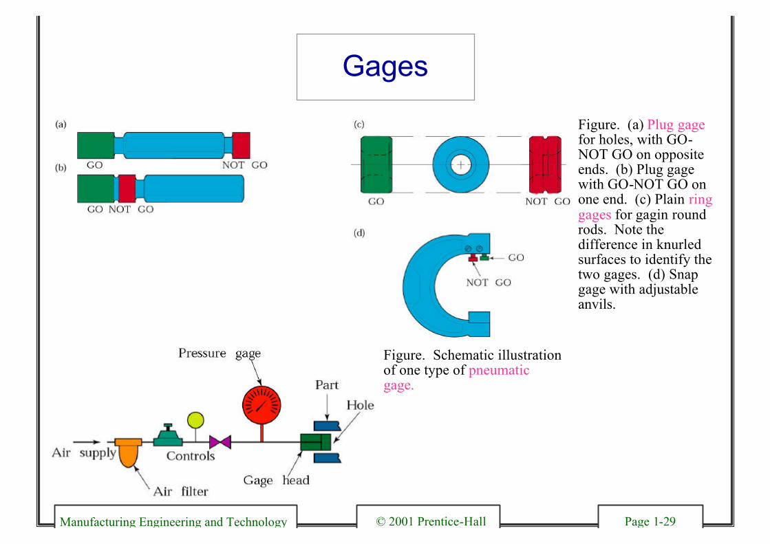
Gages

Figure. (a) Plug gagefor holes, with GO-NOT GO on opposite ends. (b) Plug gage with GO-NOT GO on one end. (c) Plain ring gages for gagin round rods. Note the difference in knurled surfaces to identify the two gages. (d) Snap gage with adjustable anvils.

Figure. Schematic illustration of one type of pneumatic gage.


Tolerance Control

Figure. Basic size, deviation, and tolerance on a shaft, according to the ISO system.

Figure . Various methods of assigning tolerances on a shaft. Source: L. E. Doyle.


Tolerances as a Function

of Size

Figure. Tolerances as a function of part size for various manufacturing processes. Note: Because many factors are involved, there is a broad range for tolerances.


Tolerances and Surface Roughnesses

Figure. Tolerances and surface roughness obtained in various manufacturing processes. These tolerances apply to a 25-mm (1-in.) workpiece dimension. Source: J. A. Schey.


Engineering Symbols

Figure. Geometric characteristic symbols to be indicated on engineering drawings of parts to be manufactured. Source: The American Society of Mechanical Engineers.


Frequency and Normal Distribution Curves

Figure. (a) A histogram of the number of shafts measured and their respective diameters. This type of curve is called frequency distribution. (b) A Normal distribution curve indicating areas within each range of standard deviation. Note: the greater the range, the higher the percentage of parts that fall within it.


Statistical Quality Control

Figure. Control charts used in statistical quality control. The process shown is in statistical control because all points fall within the lower and upper control limits. In this illustration sample size is five and the number of samples is 15.


Control Charts

Figure Control charts. (a) Process begins to become out of control because of such factors as tool wear(drift). The tool is changed and the process is then in statistical control. (b) Process parameters are not set properly; thus all parts are around the upper control limit (shift in mean). (c) Process becomes out of control because of factors such as a change in the properties of the incoming material (shift in mean).


Digital Gages with Microprocessors

Figure. Schematic illustration showing integration of digital gages with microprocessor for real-time data acquisition and SPC/SPQ capabilities. Note the examples on the CRT displays, such as frequency distribution and control charts. Source: Mitutoyo Corp.


Liquid-Penetrant and Magnetic-Particle Inspection

Figure. Sequence of operations for liquid-penetrant inspection to detect the presence of cracks and other flaws in a workpiece. Source: Metals Handbook, Desk Edition. Copyright © 1985, ASM International, Metals Park, Ohio. Used with permission.

Figure. Schematic illustration of magnetic-particle inspection of a part with a defect in it. Cracks that are in a direction parallel to the magnetic field, such as in A, would not be detected, whereas the others shown would. Cracks F, G, and H are the easiest to detect. Source: Metals Handbook, Desk Edition. Copyright © 1985, ASM International, Metals Park, Ohio. Used with permission.


Radiographic Inspection

Figure. Three methods of radiographic inspection: (a) conventional radiography, (b) digital radiography, and (c) computed tomography. Source: Courtesy of Advanced Materials and Processes, November 1990. ASM International


Eddy-Current Inspection

Figure . Changes in eddy-current flow caused by a defect in a workpiece. Source: Metals Handbook, Desk Edition. Copyright © 1985, ASM International, Metals Park, Ohio. Used with permission.


Holography

Figure. Schematic illustration of the basic optical system used in holography elements in radiography, for detecting flaws in workpieces. Source: Metals Handbook, Desk Edition. Copyright © 1985, ASM International, Metals Park, Ohio. Used with permission.


Coordinate Measuring Machine

Figure (a) Schematic illustration of one type of coordinate measuring machine. (b) Components of another type of coordinate measuring machine. These machines are available in various sizes and levels of automation and with a variety of probes (attached to the probe adapter), and are capable of measuring several features of a part. Source: Mitutoyo Corp.


Coordinate Measuring Machine

Figure A coordinate measuring machine. Brown & Sharpe Manufacturing.

chapter 4services.eng.uts.edu.au/desmanf/advman/ch04.pdf · · 2005-03-16three-dimensional...

Documents