chapter logistic regression - bradthiessen.combradthiessen.com/html5/stats/m301/logchap.pdf · ·...

CHAPTER

1414Logistic Regression

Will a patient live or die after being admitted to a hospital? Logistic regression canbe used to model categorical outcomes such as this.

14.1 The Logistic RegressionModel

14.2 Inference for LogisticRegression

IntroductionThe simple and multiple linear regression methods westudied in Chapters 10 and 11 are used to model therelationship between a quantitative response variableand one or more explanatory variables. A key assumption for these models isthat the deviations from the model fit are Normally distributed. In this chapterwe describe similar methods that are used when the response variable has onlytwo possible values.

Our response variable has only two values: success or failure, live or die, ac-ceptable or not. If we let the two values be 1 and 0, the mean is the propor-tion of ones, p = P(success). With n independent observations, we have thebinomial setting. What is new here is that we have data on an explanatory vari-able x. We study how p depends on x. For example, suppose we are studying

LOOK BACKbinomial setting,page 314whether a patient lives, (y = 1) or dies (y = 0) after being admitted to a hos-

pital. Here, p is the probability that a patient lives, and possible explanatoryvariables include (a) whether the patient is in good condition or in poor condi-tion, (b) the type of medical problem that the patient has, and (c) the age of thepatient. Note that the explanatory variables can be either categorical or quan-titative. Logistic regression is a statistical method for describing these kinds ofrelationships.1

14-1

14-2•

CHAPTER 14 • Logistic Regression

14.1 The Logistic Regression ModelBinomial distributions and oddsIn Chapter 5 we studied binomial distributions and in Chapter 8 we learnedhow to do statistical inference for the proportion p of successes in the binomialsetting. We start with a brief review of some of these ideas that we will need inthis chapter.

•

•E

XA

MP

LE 14.1 College students and binge drinking. Example 8.1 (page 489) de-

scribes a survey of 13,819 four-year college students. The researchers wereinterested in estimating the proportion of students who are frequent bingedrinkers. A male student who reports drinking five or more drinks in a row,or a female student who reports drinking four or more drinks in a row, threeor more times in the past two weeks is called a frequent binge drinker. In thenotation of Chapter 5, p is the proportion of frequent binge drinkers in theentire population of college students in four-year colleges. The number of fre-quent binge drinkers in an SRS of size n has the binomial distribution withparameters n and p. The sample size is n = 13,819 and the number of fre-quent binge drinkers in the sample is 3140. The sample proportion is

p̂ = 314013,819

= 0.2272

Logistic regressions work with odds rather than proportions. The oddsoddsare simply the ratio of the proportions for the two possible outcomes. If p̂ isthe proportion for one outcome, then 1 − p̂ is the proportion for the secondoutcome:

odds = p̂1 − p̂

A similar formula for the population odds is obtained by substituting p for p̂ inthis expression.

•

•

EX

AM

PL

E 14.2 Odds of being a binge drinker. For the binge-drinking data theproportion of frequent binge drinkers in the sample is p̂ = 0.2272, so theproportion of students who are not frequent binge drinkers is

1 − p̂ = 1 − 0.2272 = 0.7728

Therefore, the odds of a student being a frequent binge drinker are

odds = p̂1 − p̂

= 0.22720.7728

= 0.29

14.1 The Logistic Regression Model•

14-3

When people speak about odds, they often round to integers or fractions.Since 0.29 is approximately 1/3, we could say that the odds that a college stu-dent is a frequent binge drinker are 1 to 3. In a similar way, we could describethe odds that a college student is not a frequent binge drinker as 3 to 1.

USE YOUR KNOWLEDGE14.1 Odds of drawing a heart. If you deal one card from a standard deck,

the probability that the card is a heart is 0.25. Find the odds of draw-ing a heart.

14.2 Given the odds, find the probability. If you know the odds, you canfind the probability by solving the equation for odds given above forthe probability. So, p̂ = odds/(odds + 1). If the odds of an outcomeare 2 (or 2 to 1), what is the probability of the outcome?

Odds for two samplesIn Example 8.9 (page 507) we compared the proportions of frequent bingedrinkers among men and women college students using a confidence inter-val. The proportion for men is 0.260 (26.0%), and the proportion for womenis 0.206 (20.6%). The difference is 0.054, and the 95% confidence interval is(0.039, 0.069). We can summarize this result by saying, “The proportion offrequent binge drinkers is 5.4% higher among men than among women.”

Another way to analyze these data is to use logistic regression. The ex-planatory variable is gender, a categorical variable. To use this in a regression(logistic or otherwise), we need to use a numeric code. The usual way to dothis is with an indicator variable. For our problem we will use an indicator ofindicator variablewhether or not the student is a man:

x ={

1 if the student is a man0 if the student is a woman

The response variable is the proportion of frequent binge drinkers. For usein a logistic regression, we perform two transformations on this variable. First,we convert to odds. For men,

odds = p̂1 − p̂

= 0.2601 − 0.260

= 0.351

Similarly, for women we have

odds = p̂1 − p̂

= 0.2061 − 0.206

= 0.259

14-4•


USE YOUR KNOWLEDGE14.3 Energy drink commercials. A study was designed to compare two

energy drink commercials. Each participant was shown the commer-cials, A and B, in random order and asked to select the better one.There were 100 women and 140 men who participated in the study.Commercial A was selected by 45 women and by 80 men. Find theodds of selecting Commercial A for the men. Do the same for thewomen.

14.4 Find the odds. Refer to the previous exercise. Find the odds of se-lecting Commercial B for the men. Do the same for the women.

Model for logistic regressionIn simple linear regression we modeled the mean μ of the response variabley as a linear function of the explanatory variable: μ = β0 + β1x. With logisticregression we are interested in modeling the mean of the response variable pin terms of an explanatory variable x. We could try to relate p and x throughthe equation p = β0 + β1x. Unfortunately, this is not a good model. As long asβ1 �= 0, extreme values of x will give values of β0 + β1x that are inconsistent withthe fact that 0 ≤ p ≤ 1.

The logistic regression solution to this difficulty is to transform the odds(p/(1 − p)) using the natural logarithm. We use the term log odds for thislog oddstransformation. We model the log odds as a linear function of the explanatoryvariable:

log(

p1 − p

)= β0 + β1x

Figure 14.1 graphs the relationship between p and x for some different values ofβ0 and β1. For logistic regression we use natural logarithms. There are tables ofnatural logarithms, and many calculators have a built-in function for this trans-formation. As we did with linear regression, we use y for the response variable.

0 1 2 3 4 5 6 7 8 9x

10

1.0

0.9

0.8

0.7

0.6

0.5

0.4

0.3

0.2

0.1

0.0

p

β0 = – 4.0β

1 = 2.0β

β0 = – 8.0β11 == 1.61.6β β0 = – 4.0β

1 = 1.8β1 = 1.6

FIGURE 14.1 Plot of p versus xfor different logistic regressionmodels.


14-5

So for men,

y = log(odds) = log(0.351) = −1.05

and for women,

y = log(odds) = log(0.259) = −1.35

USE YOUR KNOWLEDGE14.5 Find the odds. Refer to Exercise 14.3. Find the log odds for the men

and the log odds for the women.

14.6 Find the odds. Refer to Exercise 14.4. Find the log odds for the menand the log odds for the women.

In these expressions for the log odds we use y as the observed value of theresponse variable, the log odds of being a frequent binge drinker. We are nowready to build the logistic regression model.

LOGISTIC REGRESSION MODEL

The statistical model for logistic regression is

log(

p1 − p

)= β0 + β1x

where p is a binomial proportion and x is the explanatory variable. Theparameters of the logistic model are β0 and β1.

•

•

EX

AM

PL

E 14.3 Model for binge drinking. For our binge-drinking example, thereare n = 13,819 students in the sample. The explanatory variable is gender,which we have coded using an indicator variable with values x = 1 for menand x = 0 for women. The response variable is also an indicator variable.Thus, the student is either a frequent binge drinker or not a frequent bingedrinker. Think of the process of randomly selecting a student and recordingthe value of x and whether or not the student is a frequent binge drinker.The model says that the probability (p) that this student is a frequent bingedrinker depends upon the student’s gender (x = 1 or x = 0). So there are twopossible values for p, say pmen and pwomen.

Logistic regression with an indicator explanatory variable is a very specialcase. It is important because many multiple logistic regression analyses focuson one or more such variables as the primary explanatory variables of interest.For now, we use this special case to understand a little more about the model.

The logistic regression model specifies the relationship between p and x.Since there are only two values for x, we write both equations. For men,

14-6•


log(

pmen

1 − pmen

)= β0 + β1

and for women,

log(

pwomen

1 − pwomen

)= β0

Note that there is a β1 term in the equation for men because x = 1, but it ismissing in the equation for women because x = 0.

Fitting and interpreting the logistic regression modelIn general, the calculations needed to find estimates b0 and b1 for the parame-ters β0 and β1 are complex and require the use of software. When the explana-tory variable has only two possible values, however, we can easily find the esti-mates. This simple framework also provides a setting where we can learn whatthe logistic regression parameters mean.

•

•

EX

AM

PL

E 14.4 Log odds for binge drinking. In the binge-drinking example, wefound the log odds for men,

y = log(

p̂men

1 − p̂men

)= −1.05

and for women,

y = log(

p̂women

1 − p̂women

)= −1.35

The logistic regression model for men is

log(

pmen

1 − pmen

)= β0 + β1

and for women it is

log(

pwomen

1 − pwomen

)= β0

To find the estimates of b0 and b1, we match the male and female model equa-tions with the corresponding data equations. Thus, we see that the estimateof the intercept b0 is simply the log(odds) for the women:

b0 = −1.35

and the slope is the difference between the log(odds) for the men and thelog(odds) for the women:

b1 = −1.05 − (−1.35) = 0.30

The fitted logistic regression model is

log(odds) = −1.35 + 0.30x


14-7

The slope in this logistic regression model is the difference between thelog(odds) for men and the log(odds) for women. Most people are not comfort-able thinking in the log(odds) scale, so interpretation of the results in terms ofthe regression slope is difficult. Usually, we apply a transformation to help us.With a little algebra, it can be shown that

oddsmen

oddswomen= e0.30 = 1.34

The transformation e0.30 undoes the logarithm and transforms the logistic re-gression slope into an odds ratio, in this case, the ratio of the odds that a manodds ratiois a frequent binge drinker to the odds that a woman is a frequent binge drinker.In other words, we can multiply the odds for women by the odds ratio to obtainthe odds for men:

oddsmen = 1.34 × oddswomen

In this case, the odds for men are 1.34 times the odds for women.Notice that we have chosen the coding for the indicator variable so that the

regression slope is positive. This will give an odds ratio that is greater than 1.Had we coded women as 1 and men as 0, the signs of the parameters would bereversed, the fitted equation would be log(odds) = 1.35 − 0.30x, and the oddsratio would be e−0.30 = 0.74. The odds for women are 74% of the odds for men.

USE YOUR KNOWLEDGE14.7 Find the logistic regression equation and the odds ratio. Refer

to Exercises 14.3 and 14.5. Find the logistic regression equation andthe odds ratio.

14.8 Find the logistic regression equation and the odds ratio. Referto Exercises 14.4 and 14.6. Find the logistic regression equation andthe odds ratio.

Logistic regression with an explanatory variable having two values is a veryimportant special case. Here is an example where the explanatory variable isquantitative.

•

EX

AM

PL

E 14.5 Predict whether or not the taste of the cheese is acceptable.The CHEESE data set described in the Data Appendix includes a responsevariable called “Taste” that is a measure of the quality of the cheese in theopinions of several tasters. For this example, we will classify the cheese asacceptable (tasteok = 1) if Taste ≥ 37 and unacceptable (tasteok = 0) ifTaste < 37. This is our response variable. The data set contains three ex-planatory variables: “Acetic,” “H2S,” and “Lactic.” Let’s use Acetic as theexplanatory variable. The model is

log(

p1 − p

)= β0 + β1x

14-8•


•

where p is the probability that the cheese is acceptable and x is the value ofAcetic. The model for estimated log odds fitted by software is

log(odds) = b0 + b1x = −13.71 + 2.25x

The odds ratio is eb1 = 9.48. This means that if we increase the acetic acidcontent x by one unit, we increase the odds that the cheese will be acceptableby about 9.5 times.

14.2 Inference for Logistic RegressionStatistical inference for logistic regression is very similar to statistical infer-ence for simple linear regression. We calculate estimates of the model param-eters and standard errors for these estimates. Confidence intervals are formedin the usual way, but we use standard Normal z∗-values rather than critical val-ues from the t distributions. The ratio of the estimate to the standard error isthe basis for hypothesis tests. Often the test statistics are given as the squaresof these ratios, and in this case the P-values are obtained from the chi-squaredistributions with 1 degree of freedom.

Confidence Intervals and Significance Tests

CONFIDENCE INTERVALS AND SIGNIFICANCE TESTS FORLOGISTIC REGRESSION PARAMETERS

A level C confidence interval for the slope β1 is

b1 ± z∗SEb1

The ratio of the odds for a value of the explanatory variable equal to x + 1to the odds for a value of the explanatory variable equal to x is the oddsratio.

A level C confidence interval for the odds ratio eβ1 is obtained bytransforming the confidence interval for the slope

(eb1−z∗SEb1 , eb1+z∗SEb1 )

In these expressions z∗ is the value for the standard Normal density curvewith area C between −z∗ and z∗.

To test the hypothesis H0: β1 = 0, compute the test statistic

z = b1

SEb1

The P-value for the significance test of H0 against Ha: β1 �= 0 is computedusing the fact that, when the null hypothesis is true, z has approximatelya standard Normal distribution.

14.2 Inference for Logistic Regression•

14-9

The statistic z is sometimes called a Wald statistic. Output from some sta-Wald statistictistical software reports the significance test result in terms of the square of thez statistic.

X2 = z2

This statistic is called a chi-square statistic. When the null hypothesis is true,chi-square statisticit has a distribution that is approximately a χ2 distribution with 1 degree offreedom, and the P-value is calculated as P(χ2 ≥ X2). Because the square of astandard Normal random variable has a χ2 distribution with 1 degree of free-dom, the z statistic and the chi-square statistic give the same results for statis-tical inference.

We have expressed the hypothesis-testing framework in terms of the slopeβ1 because this form closely resembles what we studied in simple linear regres-sion. In many applications, however, the results are expressed in terms of theodds ratio. A slope of 0 is the same as an odds ratio of 1, so we often express thenull hypothesis of interest as “the odds ratio is 1.” This means that the two oddsare equal and the explanatory variable is not useful for predicting the odds.

•

•

EX

AM

PL

E 14.6 Software output. Figure 14.2 gives the output from SPSS and SASfor a different binge-drinking example that is similar to the one in Example14.4. The parameter estimates are given as b0 = −1.5869 and b1 = 0.3616.The standard errors are 0.0267 and 0.0388. A 95% confidence interval for theslope is

b1 ± z∗SEb1 = 0.3616 ± (1.96)(0.0388)

= 0.3616 ± 0.0760

We are 95% confident that the slope is between 0.2856 and 0.4376. The outputprovides the odds ratio 1.436 but does not give the confidence interval. Thisis easy to compute from the interval for the slope:

(eb1−z∗SEb1 , eb1+z∗SEb1 ) = (e0.2855, e0.4376)

= (1.33, 1.55)

For this problem we would report, “College men are more likely to be frequentbinge drinkers than college women (odds ratio = 1.44, 95% CI = 1.33 to 1.55).”

In applications such as these, it is standard to use 95% for the confidencecoefficient. With this convention, the confidence interval gives us the result oftesting the null hypothesis that the odds ratio is 1 for a significance level of 0.05.If the confidence interval does not include 1, we reject H0 and conclude that theodds for the two groups are different; if the interval does include 1, the data donot provide enough evidence to distinguish the groups in this way.

The following example is typical of many applications of logistic regression.Here there is a designed experiment with five different values for the explana-tory variable.

14-10•


FIGURE 14.2 Logisticregression output from SPSS andSAS for binge-drinking data, forExample 14.6.

•

•

EX

AM

PL

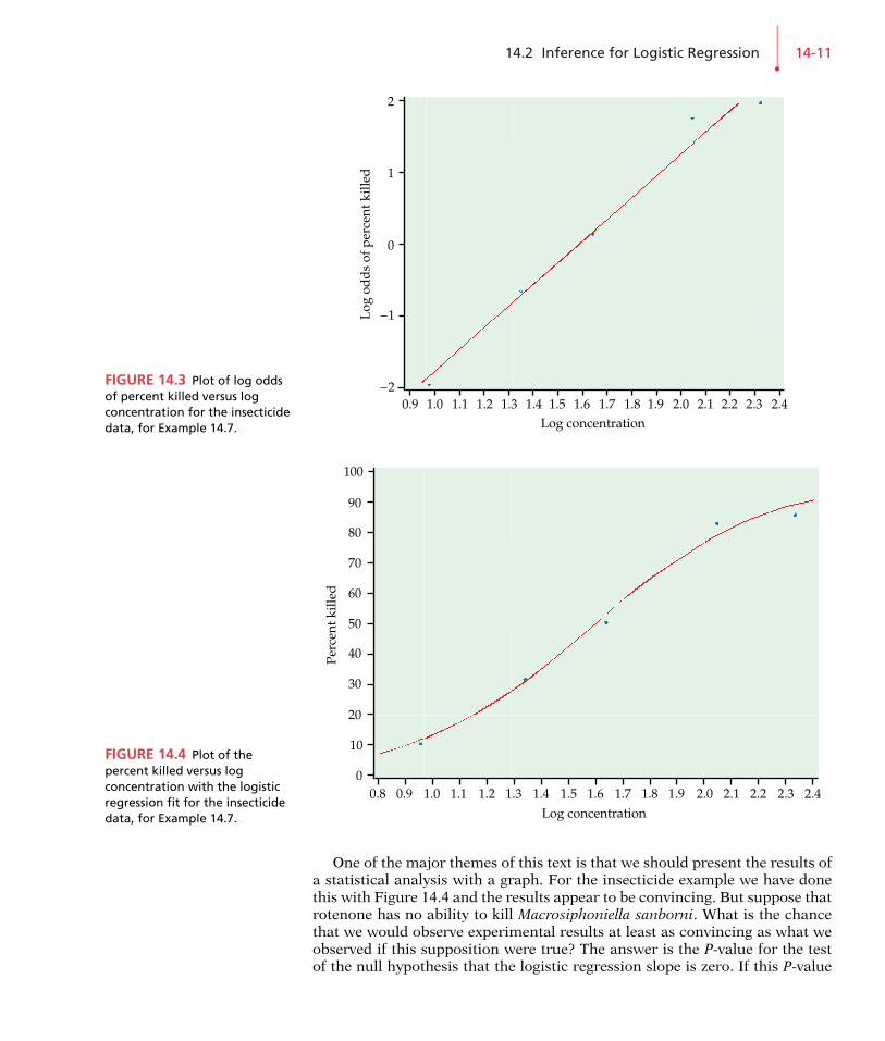
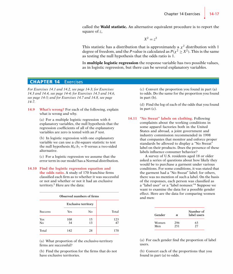
E 14.7 An insecticide for aphids. An experiment was designed to examinehow well the insecticide rotenone kills an aphid, called Macrosiphoniella san-borni, that feeds on the chrysanthemum plant.2 The explanatory variable isthe concentration (in log of milligrams per liter) of the insecticide. At eachconcentration, approximately 50 insects were exposed. Each insect was eitherkilled or not killed. We summarize the data using the number killed. The re-sponse variable for logistic regression is the log odds of the proportion killed.Here are the data:

Concentration (log) Number of insects Number killed

0.96 50 61.33 48 161.63 46 242.04 49 422.32 50 44

If we transform the response variable (by taking log odds) and use leastsquares, we get the fit illustrated in Figure 14.3. The logistic regression fit isgiven in Figure 14.4. It is a transformed version of Figure 14.3 with the fitcalculated using the logistic model.


14-11

Log

od

ds

of p

erce

nt k

illed

0.9 1.0 1.1 1.2 1.3 1.4 1.5 1.6 1.7 1.8 1.9 2.0 2.1 2.2 2.3Log concentration

2.4

2

1

0

–2

–1

FIGURE 14.3 Plot of log oddsof percent killed versus logconcentration for the insecticidedata, for Example 14.7.

Perc

ent k

illed

0.8 0.9 1.0 1.1 1.2 1.3 1.4 1.5 1.6 1.7 1.8 1.9 2.0 2.1 2.2 2.3Log concentration

2.4

100

90

80

70

60

50

40

30

20

10

0

FIGURE 14.4 Plot of thepercent killed versus logconcentration with the logisticregression fit for the insecticidedata, for Example 14.7.

One of the major themes of this text is that we should present the results ofa statistical analysis with a graph. For the insecticide example we have donethis with Figure 14.4 and the results appear to be convincing. But suppose thatrotenone has no ability to kill Macrosiphoniella sanborni. What is the chancethat we would observe experimental results at least as convincing as what weobserved if this supposition were true? The answer is the P-value for the testof the null hypothesis that the logistic regression slope is zero. If this P-value

14-12•


is not small, our graph may be misleading. Statistical inference provides whatwe need.

•

EX

AM

PL

E 14.8 Software output. Figure 14.5 gives the output from SPSS, SAS, andMinitab logistic regression analysis of the insecticide data. The model is

log(

p1 − p

)= β0 + β1x

where the values of the explanatory variable x are 0.96, 1.33, 1.63, 2.04, 2.32.From the output we see that the fitted model is

log(odds) = b0 + b1x = −4.89 + 3.10x

FIGURE 14.5 Logisticregression output from SPSS,SAS, and Minitab for theinsecticide data, for Example14.8.


14-13

•

This is the fit that we plotted in Figure 14.4. The null hypothesis that β1 = 0is clearly rejected (X2 = 64.23, P < 0.001). We calculate a 95% confidenceinterval for β1 using the estimate b1 = 3.1035 and its standard error SEb1 =0.3877 given in the output:

b1 ± z∗SEb1 = 3.1088 ± (1.96)(0.3879)

= 3.1088 ± 0.7603

We are 95% confident that the true value of the slope is between 2.34 and 3.86.The odds ratio is given on the Minitab output as 22.39. An increase of one

unit in the log concentration of insecticide (x) is associated with a 22-fold in-crease in the odds that an insect will be killed. The confidence interval for theodds is obtained from the interval for the slope:

(eb1+z∗SEb1 , eb1−z∗SEb1 ) = (e2.3485, e3.8691)

= (10.47, 47.90)

Note again that the test of the null hypothesis that the slope is 0 is the sameas the test of the null hypothesis that the odds are 1. If we were reportingthe results in terms of the odds, we could say, “The odds of killing an insectincrease by a factor of 22.4 for each unit increase in the log concentration ofinsecticide (X2 = 64.23, P < 0.001; 95% CI = 10.5 to 47.9).”

In Example 14.5 we studied the problem of predicting whether or not thetaste of cheese was acceptable using Acetic as the explanatory variable. We nowrevisit this example and show how statistical inference is an important part ofthe conclusion.

•

EX

AM

PL

E 14.9 Software output. Figure 14.6 gives the output from Minitab for alogistic regression analysis using Acetic as the explanatory variable. The fittedmodel is

log(odds) = b0 + b1x = −13.71 + 2.25x

This agrees up to rounding with the result reported in Example 14.5.From the output we see that because P = 0.029, we can reject the null hy-

pothesis that β1 = 0. The value of the test statistic is X2 = 4.79 with 1 degree offreedom. We use the estimate b1 = 2.249 and its standard error SEb1 = 1.027to compute the 95% confidence interval for β1:

FIGURE 14.6 Logisticregression output from Minitabfor the cheese data with Aceticas the explanatory variable, forExample 14.9.

14-14•


•

b1 ± z∗SEb1 = 2.249 ± (1.96)(1.027)

= 2.249 ± 2.0131

Our estimate of the slope is 2.25 and we are 95% confident that the true valueis between 0.24 and 4.26. For the odds ratio, the estimate on the output is9.48. The 95% confidence interval is

(eb1+z∗SEb1 , eb1−z∗SEb1 ) = (e0.23588, e4.26212)

= (1.27, 70.96)

We estimate that increasing the acetic acid content of the cheese by one unitwill increase the odds that the cheese will be acceptable by about 9 times. Thedata, however, do not give us a very accurate estimate. The odds ratio could beas small as a little more than 1 or as large as 71 with 95% confidence. We haveevidence to conclude that cheeses with higher concentrations of acetic acid aremore likely to be acceptable, but establishing the true relationship accuratelywould require more data.

Multiple logistic regressionThe cheese example that we just considered naturally leads us to the next topic.The data set includes three variables: Acetic, H2S, and Lactic. We examined themodel where Acetic was used to predict the odds that the cheese was accept-able. Do the other explanatory variables contain additional information thatwill give us a better prediction? We use multiple logistic regression to answermultiple logistic regressionthis question. Generating the computer output is easy, just as it was when wegeneralized simple linear regression with one explanatory variable to multiplelinear regression with more than one explanatory variable in Chapter 11. Thestatistical concepts are similar, although the computations are more complex.Here is the example.

•

EX

AM

PL

E 14.10 Software output. As in Example 14.9, we predict the odds that thecheese is acceptable. The explanatory variables are Acetic, H2S, and Lactic.Figure 14.7 gives the outputs from SPSS, SAS, and Minitab for this analysis.The fitted model is

log(odds) = b0 + b1 Acetic + b2 H2S + b3 Lactic

= −14.26 + 0.58 Acetic + 0.68 H2S + 3.47 Lactic

When analyzing data using multiple regression, we first examine the hypothe-sis that all of the regression coefficients for the explanatory variables are zero.We do the same for logistic regression. The hypothesis

H0: β1 = β2 = β3 = 0

is tested by a chi-square statistic with 3 degrees of freedom. For Minitab, thisis given in the last line of the output and the statistic is called “G.” The valueis G = 16.33 and the P-value is 0.001. We reject H0 and conclude that oneor more of the explanatory variables can be used to predict the odds that the

FIGURE 14.7 Logisticregression output from SPSS,SAS, and Minitab for the cheesedata with Acetic, H2S, and Lacticas the explanatory variables, forExample 14.10.

14-15

14-16•


•

cheese is acceptable. We now examine the coefficients for each variable andthe tests that each of these is 0. The P-values are 0.71, 0.09, and 0.19. None ofthe null hypotheses, H0: β1 = 0, H0: β2 = 0, and H0: β3 = 0, can be rejected.

Our initial multiple logistic regression analysis told us that the explanatoryvariables contain information that is useful for predicting whether or not thecheese is acceptable. Because the explanatory variables are correlated, how-ever, we cannot clearly distinguish which variables or combinations of vari-ables are important. Further analysis of these data using subsets of the threeexplanatory variables is needed to clarify the situation. We leave this work forthe exercises.

SECTION 14.2 Summary

If p̂ is the sample proportion, then the odds are p̂/(1 − p̂), the ratio of the pro-portion of times the event happens to the proportion of times the event doesnot happen.

The logistic regression model relates the log of the odds to the explanatoryvariable:

log(

pi

1 − pi

)= β0 + β1xi

where the response variables for i = 1, 2, . . . , n are independent binomial ran-dom variables with parameters 1 and pi; that is, they are independent with dis-tributions B(1, pi). The explanatory variable is x.

The parameters of the logistic model are β0 and β1.

The odds ratio is eβ1 , where β1 is the slope in the logistic regression model.

A level C confidence interval for the intercept β0 is

b0 ± z∗SEb0

A level C confidence interval for the slope β1 is

b1 ± z∗SEb1

A level C confidence interval for the odds ratio eβ1 is obtained by transform-ing the confidence interval for the slope

(eb1−z∗SEb1 , eb1+z∗SEb1 )

In these expressions z∗ is the value for the standard Normal density curve witharea C between −z∗ and z∗.

To test the hypothesis H0: β1 = 0, compute the test statistic

z = b1

SEb1

and use the fact that z has a distribution that is approximately the standard Nor-mal distribution when the null hypothesis is true. This statistic is sometimes

Chapter 14 Exercises•

14-17

called the Wald statistic. An alternative equivalent procedure is to report thesquare of z,

X2 = z2

This statistic has a distribution that is approximately a χ2 distribution with 1degree of freedom, and the P-value is calculated as P(χ2 ≥ X2). This is the sameas testing the null hypothesis that the odds ratio is 1.

In multiple logistic regression the response variable has two possible values,as in logistic regression, but there can be several explanatory variables.

CHAPTER 14 Exercises

For Exercises 14.1 and 14.2, see page 14-3; for Exercises14.3 and 14.4, see page 14-4; for Exercises 14.5 and 14.6,see page 14-5; and for Exercises 14.7 and 14.8, see page14-7.

14.9 What’s wrong? For each of the following, explainwhat is wrong and why.

(a) For a multiple logistic regression with 6explanatory variables, the null hypothesis that theregression coefficients of all of the explanatoryvariables are zero is tested with an F test.

(b) In logistic regression with one explanatoryvariable we can use a chi-square statistic to testthe null hypothesis H0: b1 = 0 versus a two-sidedalternative.

(c) For a logistic regression we assume that theerror term in our model has a Normal distribution.

14.10 Find the logistic regression equation andthe odds ratio. A study of 170 franchise firmsclassified each firm as to whether it was successfulor not and whether or not it had an exclusiveterritory.3 Here are the data:

Observed numbers of firms

Exclusive territory

Success Yes No Total

Yes 108 15 123No 34 13 47

Total 142 28 170

(a) What proportion of the exclusive-territoryfirms are successful?

(b) Find the proportion for the firms that do nothave exclusive territories.

(c) Convert the proportion you found in part (a)to odds. Do the same for the proportion you foundin part (b).

(d) Find the log of each of the odds that you foundin part (c).

14.11 “No Sweat” labels on clothing. Followingcomplaints about the working conditions insome apparel factories both in the UnitedStates and abroad, a joint government andindustry commission recommended in 1998that companies that monitor and enforce properstandards be allowed to display a “No Sweat”label on their products. Does the presence of theselabels influence consumer behavior?

A survey of U.S. residents aged 18 or olderasked a series of questions about how likely theywould be to purchase a garment under variousconditions. For some conditions, it was stated thatthe garment had a “No Sweat” label; for others,there was no mention of such a label. On the basisof the responses, each person was classified asa “label user” or a “label nonuser.”4 Suppose wewant to examine the data for a possible gendereffect. Here are the data for comparing womenand men:

Number ofGender n label users

Women 296 63Men 251 27

(a) For each gender find the proportion of labelusers.

(b) Convert each of the proportions that youfound in part (a) to odds.

14-18•


(c) Find the log of each of the odds that you foundin part (b).

14.12 Exclusive territories for franchises. Referto Exercise 14.10. Use x = 1 for the exclusiveterritories and x = 0 for the other territories.

(a) Find the estimates b0 and b1.

(b) Give the fitted logistic regression model.

(c) What is the odds ratio for exclusive territoryversus no exclusive territory?

14.13 “No Sweat” labels on clothing. Refer toExercise 14.11. Use x = 1 for women and x = 0 formen.

(a) Find the estimates b0 and b1.

(b) Give the fitted logistic regression model.

(c) What is the odds ratio for women versus men?

14.14 CH

ALLENGE Interpret the fitted model. If we apply

the exponential function to the fitted modelin Example 14.9, we get

odds = e−13.71+2.25x = e−13.71 × e2.25x

Show that, for any value of the quantitativeexplanatory variable x, the odds ratio forincreasing x by 1,

oddsx+1

oddsx

is e2.25 = 9.49. This justifies the interpretationgiven after Example 14.9.

14.15 Give a 99% confidence interval for β1. Refer toExample 14.8. Suppose that you wanted to reporta 99% confidence interval for β1. Show how youwould use the information provided in the outputsshown in Figure 14.5 to compute this interval.

14.16 Give a 99% confidence interval for the oddsratio. Refer to Example 14.8 and the outputs inFigure 14.5. Using the estimate b1 and its standarderror, find the 95% confidence interval for the oddsratio and verify that this agrees with the intervalgiven by the software.

14.17 CH

ALLENGE z and the X2 statistic. The Minitab output

in Figure 14.5 does not give the valueof X2. The column labeled “Z” provides similarinformation.

(a) Find the value under the heading “Z” forthe predictor lconc. Verify that Z is simply the

estimated coefficient divided by its standarderror. This is a z statistic that has approximatelythe standard Normal distribution if the nullhypothesis (slope 0) is true.

(b) Show that the square of z is X2. The two-sidedP-value for z is the same as P for X2.

(c) Draw sketches of the standard Normal and thechi-square distribution with 1 degree of freedom.(Hint: You can use the information in Table Fto sketch the chi-square distribution.) Indicatethe value of the z and the X2 statistics on thesesketches and use shading to illustrate the P-value.

14.18 Sexual imagery in magazine ads. Exercise 9.18(page 551) presents some results of a study abouthow advertisers use sexual imagery to appeal toyoung people. The clothing worn by the modelin each of 1509 ads was classified as “not sexual”or “sexual” based on a standardized criterion.A logistic regression was used to describe theprobability that the clothing in the ad was “notsexual” as a function of several explanatoryvariables. Here are some of the reported results:

Explanatory variable b Wald (z) statistic

Reader age 0.50 13.64Model gender 1.31 72.15Men’s magazines −0.05 0.06Women’s magazines 0.45 6.44Constant −2.32 135.92

Reader age is coded as 0 for young adult and 1for mature adult. Therefore, the coefficient of 0.50for this explanatory variable suggests that theprobability that the model clothing is not sexualis higher when the target reader age is matureadult. In other words, the model clothing is morelikely to be sexual when the target reader age isyoung adult. Model gender is coded as 0 for femaleand 1 for male. The explanatory variable men’smagazines is 1 if the intended readership is menand is 0 for women’s magazines and magazinesintended for both men and women. Women’smagazines is coded similarly.

(a) State the null and alternative hypotheses foreach of the explanatory variables.

(b) Perform the significance tests associated withthe Wald statistics.

(c) Interpret the sign of each of the statisticallysignificant coefficients in terms of the probabilitythat the model clothing is sexual.


14-19

(d) Write an equation for the fitted logisticregression model.

14.19 Interpret the odds ratios. Refer to the previousexercise. The researchers also reported odds ratios

14-20•


with 95% confidence intervals for this logisticregression model. Here is a summary:

95% ConfidenceLimits

Explanatoryvariable Odds ratio Lower Upper

Reader age 1.65 1.27 2.16Model gender 3.70 2.74 5.01Men’s magazines 0.96 0.67 1.37Women’s magazines 1.57 1.11 2.23

(a) Explain the relationship between theconfidence intervals reported here and the resultsof the Wald z significance tests that you found inthe previous exercise.

(b) Interpret the results in terms of the oddsratios.

(c) Write a short summary explaining the results.Include comments regarding the usefulness of thefitted coefficients versus the odds ratios.

14.20 What purchases will be made? A poll of 811adults aged 18 or older asked about purchasesthat they intended to make for the upcomingholiday season.5 One of the questions asked whatkind of gift they intended to buy for the person onwhom they intended to spend the most. Clothingwas the first choice of 487 people.

(a) What proportion of adults said that clothingwas their first choice?

(b) What are the odds that an adult will say thatclothing is his or her first choice?

(c) What proportion of adults said that somethingother than clothing was their first choice?

(d) What are the odds that an adult will say thatsomething other than clothing is his or her firstchoice?

(e) How are your answers to parts (a) and (d)related?

14.21 High-tech companies and stock options.Different kinds of companies compensate theirkey employees in different ways. Establishedcompanies may pay higher salaries, while newcompanies may offer stock options that will bevaluable if the company succeeds. Do high-techcompanies tend to offer stock options more oftenthan other companies? One study looked at arandom sample of 200 companies. Of these,91 were listed in the Directory of Public High

Technology Corporations, and 109 were not listed.Treat these two groups as SRSs of high-tech andnon-high-tech companies. Seventy-three of thehigh-tech companies and 75 of the non-high-techcompanies offered incentive stock options to keyemployees.6

(a) What proportion of the high-tech companiesoffer stock options to their key employees? Whatare the odds?

(b) What proportion of the non-high-techcompanies offer stock options to their keyemployees? What are the odds?

(c) Find the odds ratio using the odds for thehigh-tech companies in the numerator. Describethe result in a few sentences.

14.22 High-tech companies and stock options. Referto the previous exercise.

(a) Find the log odds for the high-tech firms. Dothe same for the non-high-tech firms.

(b) Define an explanatory variable x to have thevalue 1 for high-tech firms and 0 for non-high-techfirms. For the logistic model, we set the log oddsequal to β0 + β1x. Find the estimates b0 and b1 forthe parameters β0 and β1.

(c) Show that the odds ratio is equal to eb1 .

14.23 High-tech companies and stock options. Referto Exercises 14.21 and 14.23. Software gives0.3347 for the standard error of b1.

(a) Find the 95% confidence interval for β1.

(b) Transform your interval in (a) to a 95%confidence interval for the odds ratio.

(c) What do you conclude?

14.24 High-tech companies and stock options.Refer to Exercises 14.21 to 14.23. Repeat thecalculations assuming that you have twice asmany observations with the same proportions. Inother words, assume that there are 182 high-techfirms and 218 non-high-tech firms. The numbersof firms offering stock options are 146 for thehigh-tech group and 150 for the non-high-techgroup. The standard error of b1 for this scenario is0.2366. Summarize your results, paying particularattention to what remains the same and what isdifferent from what you found in Exercises 14.21to 14.23.

14.25 High blood pressure and cardiovasculardisease. There is much evidence that high blood


14-21

pressure is associated with increased risk of deathfrom cardiovascular disease. A major study of thisassociation examined 3338 men with high bloodpressure and 2676 men with low blood pressure.During the period of the study, 21 men in thelow-blood-pressure group and 55 in the high-blood-pressure group died from cardiovasculardisease.

(a) Find the proportion of men who died fromcardiovascular disease in the high-blood-pressuregroup. Then calculate the odds.

(b) Do the same for the low-blood-pressure group.

(c) Now calculate the odds ratio with the odds forthe high-blood-pressure group in the numerator.Describe the result in words.

14.26 Gender bias in syntax textbooks. To what extentdo syntax textbooks, which analyze the structureof sentences, illustrate gender bias? A study of thisquestion sampled sentences from 10 texts.7 Onepart of the study examined the use of the words“girl,” “boy,” “man,” and “woman.” We will callthe first two words juvenile and the last two adult.Here are data from one of the texts:

Gender n X(juvenile)

Female 60 48Male 132 52

(a) Find the proportion of the female referencesthat are juvenile. Then transform this proportionto odds.

(b) Do the same for the male references.

(c) What is the odds ratio for comparing thefemale references to the male references? (Put thefemale odds in the numerator.)

14.27 High blood pressure and cardiovasculardisease. Refer to the study of cardiovasculardisease and blood pressure in Exercise 14.25.Computer output for a logistic regression analysisof these data gives the estimated slope b1 = 0.7505with standard error SEb1 = 0.2578.

(a) Give a 95% confidence interval for the slope.

(b) Calculate the X2 statistic for testing the nullhypothesis that the slope is zero and use Table Fto find an approximate P-value.

(c) Write a short summary of the results andconclusions.

14.28 Gender bias in syntax textbooks. The datafrom the study of gender bias in syntax textbooksgiven in Exercise 14.26 are analyzed using logisticregression. The estimated slope is b1 = 1.8171 andits standard error is SEb1 = 0.3686.

(a) Give a 95% confidence interval for the slope.

(b) Calculate the X2 statistic for testing the nullhypothesis that the slope is zero and use Table Fto find an approximate P-value.

(c) Write a short summary of the results andconclusions.

14.29 High blood pressure and cardiovasculardisease. The results describing the relationshipbetween blood pressure and cardiovasculardisease are given in terms of the change in logodds in Exercise 14.27.

(a) Transform the slope to the odds and the95% confidence interval for the slope to a 95%confidence interval for the odds.

(b) Write a conclusion using the odds to describethe results.

14.30 Gender bias in syntax textbooks. The genderbias in syntax textbooks is described in the logodds scale in Exercise 14.28.

(a) Transform the slope to the odds and the95% confidence interval for the slope to a 95%confidence interval for the odds.

(b) Write a conclusion using the odds to describethe results.

14.31 Reducing the number of workers. To becompetitive in global markets, many corporationsare undertaking major reorganizations. Oftenthese involve “downsizing” or a “reduction inforce” (RIF), where substantial numbers ofemployees are terminated. Federal and variousstate laws require that employees be treatedequally regardless of their age. In particular,employees over the age of 40 years are ina “protected” class, and many allegations ofdiscrimination focus on comparing employeesover 40 with their younger coworkers. Here arethe data for a recent RIF:

Over 40

Terminated No Yes

Yes 7 41No 504 765

14-22•


(a) Write the logistic regression model for thisproblem using the log odds of a RIF as theresponse variable and an indicator for over andunder 40 years of age as the explanatory variable.

(b) Explain the assumption concerning binomialdistributions in terms of the variables in thisexercise. To what extent do you think that theseassumptions are reasonable?

(c) Software gives the estimated slope b1 = 1.3504and its standard error SEb1 = 0.4130. Transformthe results to the odds scale. Summarize theresults and write a short conclusion.

(d) If additional explanatory variables wereavailable, for example, a performance evaluation,how would you use this information to study theRIF?

14.32 Repair times for golf clubs. The Ping Companymakes custom-built golf clubs and competes inthe $4 billion golf equipment industry. To improveits business processes, Ping decided to seek ISO9001 certification.8 As part of this process, a studyof the time it took to repair golf clubs sent to thecompany by mail determined that 16% of orderswere sent back to the customers in 5 days or less.Ping examined the processing of repair ordersand made changes. Following the changes, 90%of orders were completed within 5 days. Assumethat each of the estimated percents is based ona random sample of 200 orders. Use logisticregression to examine how the odds that an orderwill be filled in 5 days or less has improved. Writea short report summarizing your results.

14.33 Education level of customers. To devise effectivemarketing strategies it is helpful to know thecharacteristics of your customers. A studycompared demographic characteristics of peoplewho use the Internet for travel arrangements andof people who do not.9 Of 1132 Internet users, 643had completed college. Among the 852 nonusers,349 had completed college. Model the log odds ofusing the Internet to make travel arrangementswith an indicator variable for having completedcollege as the explanatory variable. Summarizeyour findings.

14.34 Income level of customers. The study mentionedin the previous exercise also asked about income.Among Internet users, 493 reported income ofless than $50,000 and 378 reported income of$50,000 or more. (Not everyone answered theincome question.) The corresponding numbers fornonusers were 477 and 200. Repeat the analysis

using an indicator variable for income of $50,000or more as the explanatory variable. What do youconclude?

14.35 Alcohol use and bicycle accidents. A study ofalcohol use and deaths due to bicycle accidentscollected data on a large number of fatalaccidents.10 For each of these, the individualwho died was classified according to whether ornot there was a positive test for alcohol and bygender. Here are the data:

Gender n X(tested positive)

Female 191 27Male 1520 515

Use logistic regression to study the question ofwhether or not gender is related to alcohol use inpeople who are fatally injured in bicycle accidents.

14.36 The amount of acetic acid predicts the taste ofcheese. In Examples 14.5 and 14.9, we analyzeddata from the CHEESE data set described in theData Appendix. In those examples, we used Aceticas the explanatory variable. Run the same analysisusing H2S as the explanatory variable.

14.37 What about lactic acid? Refer to the previousexercise. Run the same analysis using Lactic asthe explanatory variable.

14.38 CH

ALLENGE Compare the analyses. For the cheese

data analyzed in Examples 14.9, 14.10,and the two exercises above, there are threeexplanatory variables. There are three differentlogistic regressions that include two explanatoryvariables. Run these. Summarize the results ofthese analyses, the ones using each explanatoryvariable alone, and the one using all threeexplanatory variables together. What do youconclude?

The following four exercises use the CSDATA data setdescribed in the Data Appendix. We examine models forrelating success as measured by the GPA to severalexplanatory variables. In Chapter 11 we used multipleregression methods for our analysis. Here, we define anindicator variable, say HIGPA, to be 1 if the GPA is 3.0 orbetter and 0 otherwise.

14.39 CH

ALLENGE Use high school grades to predict high

grade point averages. Use a logisticregression to predict HIGPA using the three highschool grade summaries as explanatory variables.


14-23

(a) Summarize the results of the hypothesis testthat the coefficients for all three explanatoryvariables are zero.

(b) Give the coefficient for high school mathgrades with a 95% confidence interval. Do thesame for the two other predictors in this model.

(c) Summarize your conclusions based on parts(a) and (b).

14.40 CH

ALLENGE Use SAT scores to predict high grade

point averages. Use a logistic regressionto predict HIGPA using the two SAT scores asexplanatory variables.

(a) Summarize the results of the hypothesis testthat the coefficients for both explanatory variablesare zero.

(b) Give the coefficient for the SAT Math scorewith a 95% confidence interval. Do the same forthe SAT Verbal score.

(c) Summarize your conclusions based on parts(a) and (b).

14.41 CH

ALLENGE Use high school grades and SAT scores

to predict high grade point averages.Run a logistic regression to predict HIGPA usingthe three high school grade summaries and thetwo SAT scores as explanatory variables. We wantto produce an analysis that is similar to that donefor the case study in Chapter 11.

(a) Test the null hypothesis that the coefficients ofthe three high school grade summaries are zero;that is, test H0: βHSM = βHSS = βHSE = 0.

(b) Test the null hypothesis that the coefficientsof the two SAT scores are zero; that is, testH0: βSATM = βSATV = 0.

(c) What do you conclude from the tests in (a)and (b)?

14.42 CH

ALLENGE Is there an effect of gender? In this

exercise we investigate the effect of genderon the odds of getting a high GPA.

(a) Use gender to predict HIGPA using a logisticregression. Summarize the results.

(b) Perform a logistic regression using gender andthe two SAT scores to predict HIGPA. Summarizethe results.

(c) Compare the results of parts (a) and (b)with respect to how gender relates to HIGPA.Summarize your conclusions.

14.43 CH

ALLENGE An example of Simpson’s paradox. Here

is an example of Simpson’s paradox, thereversal of the direction of a comparison or anassociation when data from several groups arecombined to form a single group. The data concerntwo hospitals, A and B, and whether or not patientsundergoing surgery died or survived. Here are thedata for all patients:

Hospital A Hospital B

Died 63 16Survived 2037 784

Total 2100 800

And here are the more detailed data where thepatients are categorized as being in good conditionor poor condition:

Good condition



Total 600 600

Poor condition



Total 1500 200

(a) Use a logistic regression to model the odds ofdeath with hospital as the explanatory variable.Summarize the results of your analysis and givea 95% confidence interval for the odds ratio ofHospital A relative to Hospital B.

(b) Rerun your analysis in (a) using hospitaland the condition of the patient as explanatoryvariables. Summarize the results of your analysisand give a 95% confidence interval for the oddsratio of Hospital A relative to Hospital B.

(c) Explain Simpson’s paradox in terms of yourresults in parts (a) and (b).

14-24•


CHAPTER 14 Notes

1. Logistic regression models for the general case wherethere are more than two possible values for the responsevariable have been developed. These are considerably morecomplicated and are beyond the scope of our present study.For more information on logistic regression, see A. Agresti,An Introduction to Categorical Data Analysis, 2nd ed., Wiley,2002; and D. W. Hosmer and S. Lemeshow, Applied LogisticRegression, 2nd ed., Wiley, 2000.

2. This example is taken from a classic text written by acontemporary of R. A. Fisher, the person who developedmany of the fundamental ideas of statistical inference thatwe use today. The reference is D. J. Finney, Probit Analysis,Cambridge University Press, 1947. Although not includedin the analysis, it is important to note that the experimentincluded a control group that received no insecticide. Noaphids died in this group. We have chosen to call the re-sponse “dead.” In Finney’s book the category is describedas “apparently dead, moribund, or so badly affected as tobe unable to walk more than a few steps.” This is an earlyexample of the need to make careful judgments when defin-ing variables to be used in a statistical analysis. An insectthat is “unable to walk more than a few steps” is unlikely toeat very much of a chrysanthemum plant!

3. From P. Azoulay and S. Shane, “Entrepreneurs, con-tracts, and the failure of young firms,” Management Science,

47 (2001), pp. 337–358.

4. Marsha A. Dickson, “Utility of no sweat labels for ap-parel customers: profiling label users and predicting theirpurchases,” Journal of Consumer Affairs, 35 (2001), pp. 96–119.

5. The poll is part of the American Express Retail IndexProject and is reported in Stores, December 2000, pp. 38–40.

6. Based on Greg Clinch, “Employee compensation andfirms’ research and development activity,” Journal of Ac-counting Research, 29 (1991), pp. 59–78.

7. Monica Macaulay and Colleen Brice, “Don’t touchmy projectile: gender bias and stereotyping in syntacticexamples,” Language, 73, no. 4 (1997), pp. 798–825.

8. Based on Robert T. Driescher, “A quality swing withPing,” Quality Progress, August 2001, pp. 37–41.

9. Karin Weber and Weley S. Roehl, “Profiling peoplesearching for and purchasing travel products on the WorldWide Web,” Journal of Travel Research, 37 (1999), pp. 291–298.

10. Guohua Li and Susan P. Baker, “Alcohol in fatallyinjured bicyclists,” Accident Analysis and Prevention, 26(1994), pp. 543–548.

chapter logistic regression - bradthiessen.combradthiessen.com/html5/stats/m301/logchap.pdf · ·...

Documents