chapter 9 multiple importance sampling - computer graphics · chapter 9 multiple importance...
TRANSCRIPT
Chapter 9
Multiple Importance Sampling
We introduce a technique called multiple importance sampling that can greatly increase the
reliability and efficiency of Monte Carlo integration. It is based on the idea of using more
than one sampling technique to evaluate a given integral, and combining the sample values
in a provably good way.
Our motivation is that most numerical integration problems in computer graphics are
“difficult”, i.e. the integrands are discontinuous, high-dimensional, and/or singular. Given
a problem of this type, we would like to design a sampling strategy that gives a low-variance
estimate of the integral. This is complicated by the fact that the integrand usually depends on
parameters whose values are not known at the time an integration strategy is designed (e.g.
material properties, the scene geometry, etc.) It is difficult to design a sampling strategy that
works reliably in this situation, since the integrand can take on a wide variety of different
shapes as these parameters vary.
In this chapter, we explore the general problem of constructing low-variance estimators
by combining samples from several different sampling techniques. We do not construct new
sampling techniques — we assume that these are given to us. Instead, we look for better
ways to combine the samples, by computing weighted combinations of the sample values.
We show that there is a large class of unbiased estimators of this type, which can be pa-
rameterized by a set of weighting functions. Our goal is to find an estimator with minimum
variance, by choosing these weighting functions appropriately.
A good solution to this problem turns out to be surprisingly simple. We show how to
251

252 CHAPTER 9. MULTIPLE IMPORTANCE SAMPLING
combine samples from several techniques in a way that is provably good, both theoretically
and practically. This allows us to construct Monte Carlo estimators that have low variance
for a broad class of integrands — we call such estimators robust. The significance of our
methods is not that we can take several bad sampling techniques and concoct a good one
out of them, but rather that we can take several potentially good techniques and combine
them so that the strengths of each are preserved.
This chapter is organized as follows. We start with an extended example to motivate our
variance reduction techniques (Section 9.1). Specifically, we consider the problem of com-
puting the appearance of a glossy surface illuminated by an area light source. Next, in Sec-
tion 9.2 we explain the multiple importance sampling framework. Several models for taking
and combining the sampling are described, and we present theoretical results showing that
these techniques are provably close to optimal (proofs may be found in Appendix 9.A). In
Section 9.3, we show that these techniques work well in practice, by presenting images and
numerical measurements for two specific applications: the glossy highlights problem men-
tioned above, and the “final gather” pass that is used in some multi-pass algorithms. Finally,
Section 9.4 discusses of a number of tradeoffs and open issues related to our work.
9.1 Application: glossy highlights from area light sources
We have chosen a problem from distribution ray tracing to illustrate our techniques. Given
a glossy surface illuminated by an area light source, the goal is to determine its appearance.
These “glossy highlights” are commonly evaluated in one of two ways: either by sampling
the light source, or sampling the BSDF. We show that each method works very well in some
situations, but fails in others. Obviously, we would prefer a sampling strategy that works
well all the time. Later in this chapter, we will show how multiple importance sampling can
be applied to solve this problem.
9.1.1 The glossy highlights problem
Consider an area light source�
that illuminates a nearby glossy surface (see Figure 9.1). The
goal is to determine the appearance of this surface, i.e. to evaluate the radiance ��������� ������

9.1. GLOSSY HIGHLIGHTS FROM AREA LIGHT SOURCES 253
x'
x
N
N
x''
θ'i
θo
ω'iω'o
glossy surface
lightspherical
source
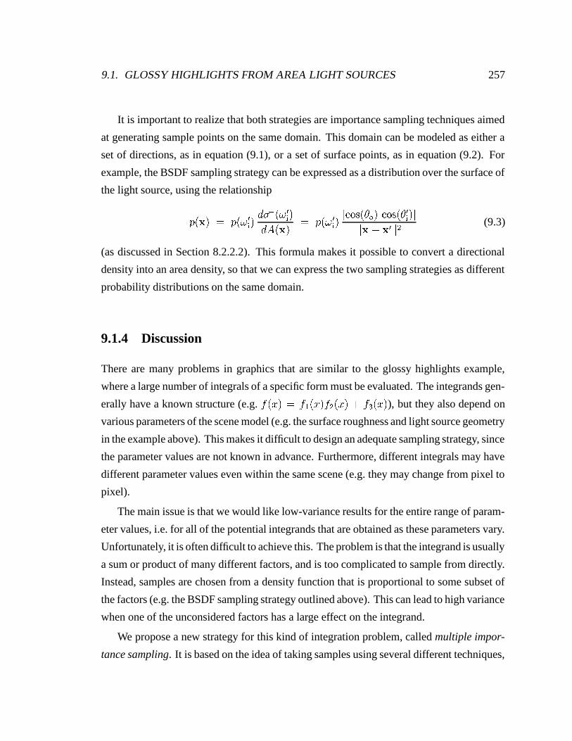
Figure 9.1: Geometry for the glossy highlights computation. The radiance for each viewingray is obtained by integrating the light that is emitted by the source, and reflected from theglossy surface toward the eye.
that leaves the surface toward the eye. Mathematically, this is determined by the scattering
equation (3.12):
� � � � � � �� � � �������� � � � �� � � �� � ����� � � � � � �� ������� ��� �� � (9.1)
where ����� � represents the incident radiance due to the area light source�
.
We will examine a family of integration problems of this form, obtained by varying the
size of the light source and the glossiness of the surface. In particular, we consider spherical
light sources of varying radii, and glossy materials that have a surface roughness parame-
ter ( � ) that determines how sharp or fuzzy the reflections are. Smooth surfaces ( � � � )correspond to highly polished, mirror-like reflections, while rough surfaces ( � ��� ) corre-
spond to diffuse reflection. It is possible to simulate a variety of surface finishes by using
intermediate roughness values in the range ��� � ��� .9.1.2 Two sampling strategies
There are two common strategies for Monte Carlo evaluation of the scattering equation
(9.1), which we call sampling the BSDF and sampling the light source. The results of these
techniques are demonstrated in Figure 9.2(a) and Figure 9.2(b) respectively, over a range of
different light source sizes and surface finishes. We will first describe these two strategies,
254 CHAPTER 9. MULTIPLE IMPORTANCE SAMPLING
and then examine why each one has high variance in some situations.
Sampling the BSDF. To sample the BSDF, an incident direction � �� is randomly chosen
according to a predetermined density � ��� �� � . Normally, this density is chosen to be propor-
tional to the BSDF (or some convenient approximation), i.e.
� ��� �� ����� � � � �� � � ����
where � is measured with respect to projected solid angle. To estimate the scattering equa-
tion (9.1), an estimate of the usual form
� ��� � � � �� ����� � � � �� � � �� � ����� � � � � � �� �
� ��� �� �is used. The emitted radiance � � � � � � � � �� � is evaluated by casting a ray to find the corre-
sponding point on the light source. Note that some rays may miss the light source�
, in
which case they do not contribute to the highlight calculation. The image in Figure 9.2(a)
was computed using this strategy.
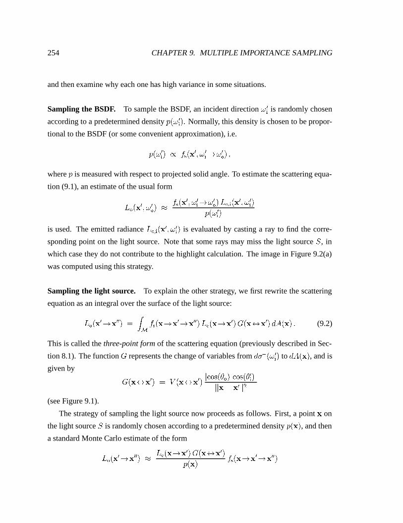
Sampling the light source. To explain the other strategy, we first rewrite the scattering
equation as an integral over the surface of the light source:
� ����� � � � � � � � ��� ��� � � � � � � � � ����� � � � � ��� ���� � � ���� ��� � � (9.2)
This is called the three-point form of the scattering equation (previously described in Sec-
tion 8.1). The function � represents the change of variables from ��� � ��� �� � to �� � � � , and is
given by
� � �� � � � � � ���� � � �� ����� ��� � � ����� ��� �� � �� ��� � � ���
(see Figure 9.1).
The strategy of sampling the light source now proceeds as follows. First, a point � on
the light source�
is randomly chosen according to a predetermined density � � � � , and then
a standard Monte Carlo estimate of the form
� � ��� � � � � � ��� ��� � � � � � ��� ���� � � �� � � �
�� � � � � � � � � �
9.1. GLOSSY HIGHLIGHTS FROM AREA LIGHT SOURCES 255
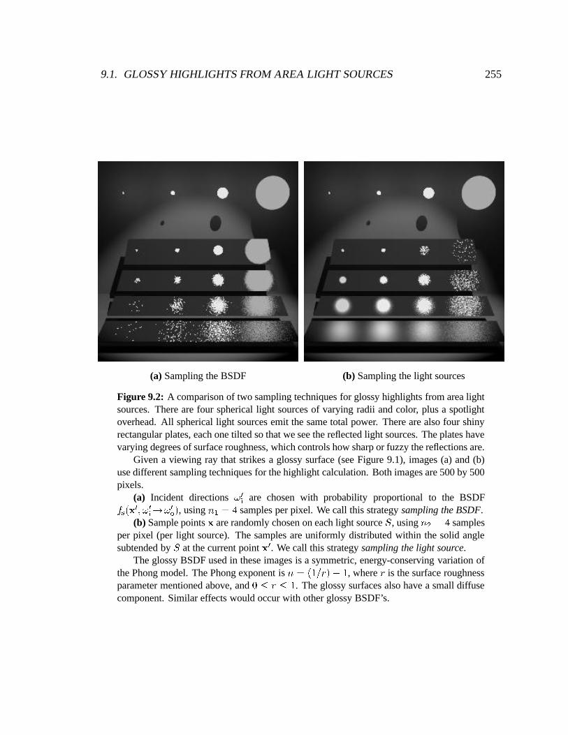
(a) Sampling the BSDF (b) Sampling the light sources
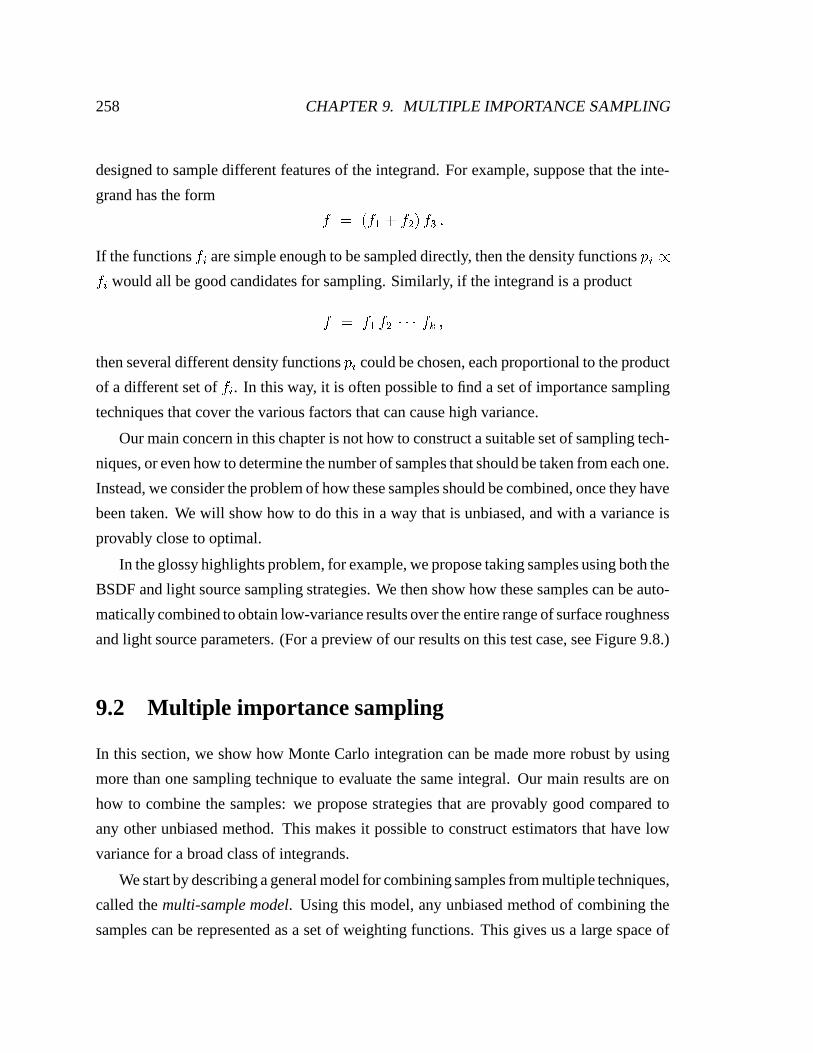
Figure 9.2: A comparison of two sampling techniques for glossy highlights from area lightsources. There are four spherical light sources of varying radii and color, plus a spotlightoverhead. All spherical light sources emit the same total power. There are also four shinyrectangular plates, each one tilted so that we see the reflected light sources. The plates havevarying degrees of surface roughness, which controls how sharp or fuzzy the reflections are.
Given a viewing ray that strikes a glossy surface (see Figure 9.1), images (a) and (b)use different sampling techniques for the highlight calculation. Both images are 500 by 500pixels.
(a) Incident directions � �� are chosen with probability proportional to the BSDF� ���� ��� � ���� � �� , using � ����� samples per pixel. We call this strategy sampling the BSDF.(b) Sample points
�are randomly chosen on each light source � , using � � ��� samples
per pixel (per light source). The samples are uniformly distributed within the solid anglesubtended by � at the current point
�� . We call this strategy sampling the light source.
The glossy BSDF used in these images is a symmetric, energy-conserving variation ofthe Phong model. The Phong exponent is ��� �������
���, where
�is the surface roughness
parameter mentioned above, and ��� � � �. The glossy surfaces also have a small diffuse
component. Similar effects would occur with other glossy BSDF’s.
256 CHAPTER 9. MULTIPLE IMPORTANCE SAMPLING
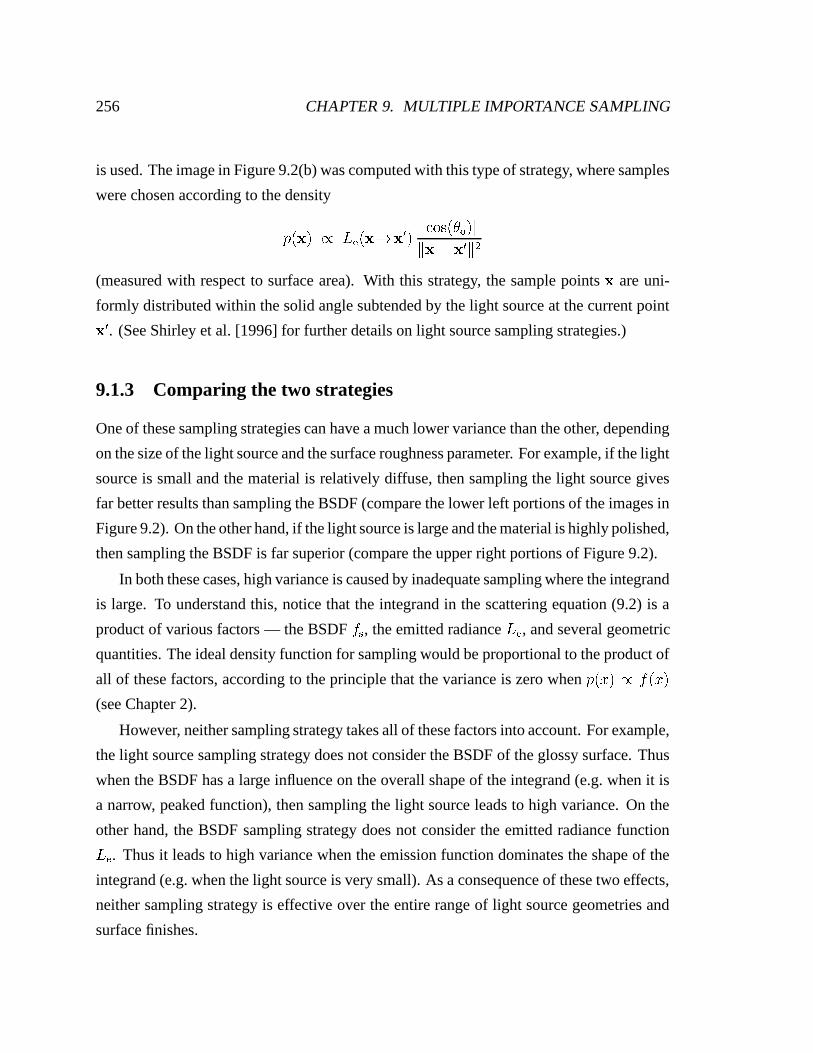
is used. The image in Figure 9.2(b) was computed with this type of strategy, where samples
were chosen according to the density
� ��� ��� ��� ��� � � � �� ��� � ��� � � �� � � � � ���
(measured with respect to surface area). With this strategy, the sample points � are uni-
formly distributed within the solid angle subtended by the light source at the current point
� � . (See Shirley et al. [1996] for further details on light source sampling strategies.)
9.1.3 Comparing the two strategies
One of these sampling strategies can have a much lower variance than the other, depending
on the size of the light source and the surface roughness parameter. For example, if the light
source is small and the material is relatively diffuse, then sampling the light source gives
far better results than sampling the BSDF (compare the lower left portions of the images in
Figure 9.2). On the other hand, if the light source is large and the material is highly polished,
then sampling the BSDF is far superior (compare the upper right portions of Figure 9.2).
In both these cases, high variance is caused by inadequate sampling where the integrand
is large. To understand this, notice that the integrand in the scattering equation (9.2) is a
product of various factors — the BSDF��
, the emitted radiance � � , and several geometric
quantities. The ideal density function for sampling would be proportional to the product of
all of these factors, according to the principle that the variance is zero when � ��� � ����� �
(see Chapter 2).
However, neither sampling strategy takes all of these factors into account. For example,
the light source sampling strategy does not consider the BSDF of the glossy surface. Thus
when the BSDF has a large influence on the overall shape of the integrand (e.g. when it is
a narrow, peaked function), then sampling the light source leads to high variance. On the
other hand, the BSDF sampling strategy does not consider the emitted radiance function
��� . Thus it leads to high variance when the emission function dominates the shape of the
integrand (e.g. when the light source is very small). As a consequence of these two effects,
neither sampling strategy is effective over the entire range of light source geometries and
surface finishes.
9.1. GLOSSY HIGHLIGHTS FROM AREA LIGHT SOURCES 257
It is important to realize that both strategies are importance sampling techniques aimed
at generating sample points on the same domain. This domain can be modeled as either a
set of directions, as in equation (9.1), or a set of surface points, as in equation (9.2). For
example, the BSDF sampling strategy can be expressed as a distribution over the surface of
the light source, using the relationship
� ��� � � � ��� �� � ��� � ��� �� ��� ��� �� � ��� �� � � ����� ��� � � ��� � ��� �� � �� � � � � ��� (9.3)
(as discussed in Section 8.2.2.2). This formula makes it possible to convert a directional
density into an area density, so that we can express the two sampling strategies as different
probability distributions on the same domain.
9.1.4 Discussion
There are many problems in graphics that are similar to the glossy highlights example,
where a large number of integrals of a specific form must be evaluated. The integrands gen-
erally have a known structure (e.g.���� � � � � ��� � � � � � � �
�� ��� � ), but they also depend on
various parameters of the scene model (e.g. the surface roughness and light source geometry
in the example above). This makes it difficult to design an adequate sampling strategy, since
the parameter values are not known in advance. Furthermore, different integrals may have
different parameter values even within the same scene (e.g. they may change from pixel to
pixel).
The main issue is that we would like low-variance results for the entire range of param-
eter values, i.e. for all of the potential integrands that are obtained as these parameters vary.
Unfortunately, it is often difficult to achieve this. The problem is that the integrand is usually
a sum or product of many different factors, and is too complicated to sample from directly.
Instead, samples are chosen from a density function that is proportional to some subset of
the factors (e.g. the BSDF sampling strategy outlined above). This can lead to high variance
when one of the unconsidered factors has a large effect on the integrand.
We propose a new strategy for this kind of integration problem, called multiple impor-
tance sampling. It is based on the idea of taking samples using several different techniques,
258 CHAPTER 9. MULTIPLE IMPORTANCE SAMPLING
designed to sample different features of the integrand. For example, suppose that the inte-
grand has the form � � �� � �
� � � � � �If the functions
�� are simple enough to be sampled directly, then the density functions � � ��
� would all be good candidates for sampling. Similarly, if the integrand is a product� � � � � ������� � � then several different density functions � � could be chosen, each proportional to the product
of a different set of�� . In this way, it is often possible to find a set of importance sampling
techniques that cover the various factors that can cause high variance.
Our main concern in this chapter is not how to construct a suitable set of sampling tech-
niques, or even how to determine the number of samples that should be taken from each one.
Instead, we consider the problem of how these samples should be combined, once they have
been taken. We will show how to do this in a way that is unbiased, and with a variance is
provably close to optimal.
In the glossy highlights problem, for example, we propose taking samples using both the
BSDF and light source sampling strategies. We then show how these samples can be auto-
matically combined to obtain low-variance results over the entire range of surface roughness
and light source parameters. (For a preview of our results on this test case, see Figure 9.8.)
9.2 Multiple importance sampling
In this section, we show how Monte Carlo integration can be made more robust by using
more than one sampling technique to evaluate the same integral. Our main results are on
how to combine the samples: we propose strategies that are provably good compared to
any other unbiased method. This makes it possible to construct estimators that have low
variance for a broad class of integrands.
We start by describing a general model for combining samples from multiple techniques,
called the multi-sample model. Using this model, any unbiased method of combining the
samples can be represented as a set of weighting functions. This gives us a large space of

9.2. MULTIPLE IMPORTANCE SAMPLING 259
possible combination strategies to explore, and a uniform way to represent them.
We then present a provably good strategy for combining the samples, which we call the
balance heuristic. We show that this method gives a variance that is smaller than any other
unbiased combination strategy, to within a small additive term. The method is simple and
practical, and can make Monte Carlo calculations significantly more robust. We also pro-
pose several other combination strategies, which are basically refinements of the balance
heuristic: they retain its provably good behavior in general, but are designed to have lower
variance in a common special case. For this reason, they are often preferable to the balance
heuristic in practice.
We conclude by considering a different model for how the samples are taken and com-
bined, called the one-sample model. Under this model, the integral is estimated by choosing
one of the � sampling techniques at random, and then taking a single sample from it. Again
we consider how to minimize variance by weighting the samples, and we show that for this
model the balance heuristic is optimal.
9.2.1 The multi-sample model
In order to prove anything about our methods, there must be a precise model for how the
samples are taken and combined. For most of this chapter, we will use the multi-sample
model described below. This model allows any unbiased combination strategy to be en-
coded as a set of weighting functions.
We consider the evaluation of an integral������ ����� ��� �
where the domain � , the function���
� � � � , and the measure � are all given. We are
also given a set of � different sampling techniques on the domain � , whose corresponding
density functions are labeled � � , � � � , � . We assume that only the following operations are
available:
� Given any point � ��� ,�� � � and � � � � � can be evaluated.
� It is possible to generate a sample � distributed according to any of the � � .
260 CHAPTER 9. MULTIPLE IMPORTANCE SAMPLING
To estimate the integral, several samples are generated using each of the given tech-
niques. We let � � denote the number of samples from � � , where � ��� � , and we let � ��� � �denote the total number of samples. We assume that the number of samples from each tech-
nique is fixed in advance, before any samples are taken. (We do not consider the problem of
how to allocate samples among the techniques; this is an interesting problem in itself, which
will be discussed further in Section 9.4.2.) The samples from technique � are denoted � � � � ,for � � � � � � � � . All samples are assumed to be independent, i.e. new random bits are
generated to control the selection of each one.
9.2.1.1 The multi-sample estimator
We now examine how the samples � � � � can be used to estimate the desired integral. Our
goal is generality: given any unbiased way of combining the samples, there should be a
way to represent it. To do this, we consider estimators that allow the samples to be weighted
differently, depending on which technique � � they were sampled from. Each estimator has
an associated set of weighting functions � � , � � � , � which give the weight � � ��� � for each
sample � drawn from � � . The multi-sample estimator is then given by
� ��� �
�� �� � � � � � � � � � � �
�� � � � � �
� � � � � � � � � (9.4)
This formula can be thought of as a weighted sum of the estimators�� � � � � ��� � � � � � � � � that
would be obtained by using each sampling technique � � on its own. Notice that the weights
are not constant, but can vary as a function of the sample point � � � � .For this estimate to be unbiased, the weighting functions � � must satisfy the following
two conditions:
(W1)��� � � � � � �
� � whenever�� � ���� � , and
(W2) � � ��� � ��� whenever � � � � � � � �These conditions imply the following corollary: at any point where
�� � ���� � , at least one
of the � � ��� � must be positive (i.e., at least one sampling technique must be able to gener-
ate samples there). Thus on the other hand, it is not necessary for every � � to sample the
9.2. MULTIPLE IMPORTANCE SAMPLING 261
whole domain; it is allowable for some of the � � to be specialized sampling techniques that
concentrate on specific regions of the integrand.1
Given that (W1) and (W2) hold, the following lemma states that
is unbiased:
Lemma 9.1. Let
be any estimator of the form (9.4), where � � � � for all � , and the weight-
ing functions � � satisfy conditions (W1) and (W2). Then
��� �� � ������ ����� � � � �
Proof.
��� �� � ��� �
�� �
� � �
�� �
� ��� ��� � �
� � ��� � � � � � ��� � ��� �� �
���� � � � ��� �
�� � ����� ��� �
� ������ ����� � � � �
The remainder of this section is devoted to showing the generality of the multi-sample
model. We show that by choosing the weighting functions appropriately, it is possible to
represent virtually any unbiased combination strategy. To make this more concrete, we first
give some examples of possible strategies, and show how to represent them by weighting
functions. We then show how the multi-sample estimator can be rewritten in a different
form that makes its generality more obvious. This leads up to Section 9.2.2, where we will
describe a new combination strategy that has provably good performance compared to all
strategies that the multi-sample model can represent.
9.2.1.2 Examples of weighting functions
Suppose that there are three sampling techniques � � , � � , and � � , and that a single sample � � � �is taken from each one ( � � � � � � � � � � ). First, consider the case where the weighting
1If � is allowed to contain Dirac distributions, note that (W2) should be modified to state that � ���������whenever ������������������ is not finite. To relate this to graphics, consider a mirror which also reflects some lightdiffusely. The modified (W2) states that samples from the diffuse component cannot be used to estimate thespecular contribution, since this corresponds to the situation where ������� contains a Dirac distribution ���� �! �"#� , but �$����� does not.)

262 CHAPTER 9. MULTIPLE IMPORTANCE SAMPLING
functions are constant over the whole domain � . This leads to the estimator
� � ��� � � � � �
� � � � � � � � � � ��� � � � � �
� � � � � � � � � � �
�� � � � � �
� � � � � � � � where the � � sum to one. This estimator is simply a weighted combination of the estimators� � �
� � � � � � � � � � � � � � � that would be obtained by using each of the sampling techniques
alone. Unfortunately, this combination strategy does not work very well: if any of the given
sampling techniques is bad (i.e. the corresponding estimator� has high variance), then
will have high variance as well, since
� � �� � � � � � � � � � � � � � � � � � � � �� �
Another possible combination strategy is to partition the domain among the sampling
techniques. To do this, the integral is written in the form������ ����� ��� � �
��� ��� �� � ����� ��� �
where the � � are non-overlapping regions whose union is � . The integral is then estimated
in each region � � separately, using samples from just one technique � � . In terms of weighting
functions, this is represented by letting
� � ��� � � �� � � if � � � � � otherwise �
This combination strategy is used a great deal in computer graphics; however, some-
times it does not work very well due to the simple partitioning rules that are used. For
example, it is common to evaluate the scattering equation by dividing the scene into light
source regions and non-light-source regions, which are sampled using different techniques
(e.g. sampling ��� vs. sampling the BSDF). Depending on the geometry and materials of the
scene, this fixed partitioning can lead to a much higher variance than necessary (as we saw
in the glossy highlights example).
Another combination technique that is often used in graphics is to write the integrand
as a sum� � ��� � , and use a different sampling technique to estimate the contribution of
each � � . For example, this occurs when the BSDF is split into diffuse, glossy, and specular
9.2. MULTIPLE IMPORTANCE SAMPLING 263
components, whose contributions are estimated separately (by sampling from density func-
tions � � � � � ). As before, it is straightforward to represent this strategy as a set of weighting
functions.
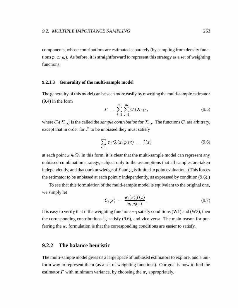
9.2.1.3 Generality of the multi-sample model
The generality of this model can be seen more easily by rewriting the multi-sample estimator
(9.4) in the form �
��� �� � � ��� � � � � � � � (9.5)
where �� � � � � � � is the called the sample contribution for � � � � . The functions �
� are arbitrary,
except that in order for
to be unbiased they must satisfy
��� � � � � � ��� � � � ��� �
� �� � � (9.6)
at each point � � � . In this form, it is clear that the multi-sample model can represent any
unbiased combination strategy, subject only to the assumptions that all samples are taken
independently, and that our knowledge of�
and � � is limited to point evaluation. (This forces
the estimator to be unbiased at each point � independently, as expressed by condition (9.6).)
To see that this formulation of the multi-sample model is equivalent to the original one,
we simply let
�� ��� � � � � ��� �
�� � �
� � � � ��� � � (9.7)
It is easy to verify that if the weighting functions � � satisfy conditions (W1) and (W2), then
the corresponding contributions �� satisfy (9.6), and vice versa. The main reason for pre-
ferring the � � formulation is that the corresponding conditions are easier to satisfy.
9.2.2 The balance heuristic
The multi-sample model gives us a large space of unbiased estimators to explore, and a uni-
form way to represent them (as a set of weighting functions). Our goal is now to find the
estimator
with minimum variance, by choosing the � � appropriately.

264 CHAPTER 9. MULTIPLE IMPORTANCE SAMPLING
We will show that the following weighting functions are a good choice:�� � ��� � � � � � � ��� �� � � � � � ��� � � (9.8)
We call this strategy the balance heuristic.2 The key feature of the balance heuristic is that
no other combination strategy is much better, as stated by the following theorem:
Theorem 9.2. Let�
, � � , and � � be given, for � � � � � � � . Let
be any unbiased estimator
of the form (9.4), and let�
be the estimator that uses the weighting functions�� � (the balance
heuristic). Then� � ��� � � � ���� � ������ � � � � �
� � � � � � (9.9)
where � � ��� �� � ��� ���is the quantity to be estimated. (A proof is given in Appendix 9.A.)
According to this result, no other combination strategy can significantly improve upon
the balance heuristic. That is, suppose that we let��
denote the best possible combination
strategy for a particular problem (i.e. for a given choice of the�
, � � , and � � ). In general,
we have no way of knowing what this strategy is: for example, suppose that one of the � �is exactly proportional to
�, so that the best strategy is to ignore any samples taken with the
other techniques, and use only the samples from � � . We cannot hope to discover this fact
from a practical point of view, since our knowledge of�
and � � is limited to point sampling
and evaluation. Nevertheless, even compared to this unknown optimal strategy��
, the bal-
ance heuristic is almost as good: its variance is worse by at most the term on the right-hand
side of (9.9).
To give some intuition about this upper bound on the “variance gap”, suppose that there
are just two sampling techniques, and that � � � � � �� samples are taken from each one. In
this case, the variance of the balance heuristic is optimal to within an additive term of � � ��� .In familiar graphics terms, this corresponds to the variance obtained by sending 8 shadow
2The name refers to the fact that the sample contributions are “balanced” so that they are the same for alltechniques � : �
����� � � ����� �������� � ����� � ���������� � � � � �������That is, the contribution
� ��� �� � � of a sample � �� � does not depend on which technique � generated it.

9.2. MULTIPLE IMPORTANCE SAMPLING 265
rays to an area light source that is 50% occluded. Furthermore, notice that the variance gap
goes to zero as the number of samples from each technique is increased. On the other hand,
if a poor combination strategy is used then the variance can be larger than optimal by an
arbitrary amount. This is essentially what we observed in the glossy highlights images of
Figure 9.2: if the wrong samples are used to estimate the integral, the variance can be tens
or hundreds of times larger than � � .Furthermore, the balance heuristic is practical to implement. The main requirement for
evaluating the weighting functions�� � is that given any point � , we must be able to evaluate
the probability densities � � ��� � for all � . This situation is different than for the usual esti-
mator�� � � � � � � � , where it is only necessary to evaluate � � � � for sample points generated
using � . The balance heuristic requires slightly more than this: given a sample � � � � gener-
ated using technique � � , we also need to evaluate the probabilities � � � � � � � � with which all of
the other � � � techniques generate that sample point. It is usually straightforward to do this;
it is just a matter of reorganizing the routines that compute probabilities, and expressing all
densities with respect to the same measure.
For example, consider the glossy highlights problem of Section 9.1. To evaluate the
weighting function�� � for each sample point � , we compute the probability density for gen-
erating � using both sampling techniques. Thus if � was generated by sampling the light
source, then we also compute the probability density for generating the same point � by
sampling the BSDF (as discussed in Section 9.1.3). Note that the cost of computing these
extra probabilities is insignificant compared to the other calculations involved, such as ray
casting; details will be given in Section 9.3.
9.2.2.1 A simple interpretation of the balance heuristic
By writing the balance heuristic in a different form, we will show that it is actually a very
natural way to combine samples from multiple techniques.
To do this, we insert the weighting functions�� � into the multi-sample estimator (9.4),
yielding � � ��� �
�� �� � � �
� � � � � � � � � � �� � � � � � � � � � � � �� � � � � �
� � � � � � � �
266 CHAPTER 9. MULTIPLE IMPORTANCE SAMPLING
� ��� �
� � � �
�� � � � � �� � � � � � � � � � � �
� ��
��� �
� � � �
�� � � � � �� ��� � � � � � � � � � (9.10)
where � � � � � � is the total number of samples, and � � � � � � � is the fraction of samples
from � � .In this form, the balance heuristic corresponds to a standard Monte Carlo estimator of
the form�� � . This can be seen more easily by rewriting the denominator of (9.10) as�� ��� � �
� � � � � � � � � � (9.11)
which we call the combined sample density. The quantity�� ��� � represents the probability
density for sampling the given point � , averaged over the entire sequence of � samples.3
Thus, the balance heuristic is natural way to combine the samples. It has the form of a
standard Monte Carlo estimator, where the denominator�� represents the average distribu-
tion of the whole group of samples to which it is applied. Pseudocode for this estimator is
given in Figure 9.3. However, it is important to realize that the main advantage of this esti-
mator is not that it is simple or standard, but that it has provably good performance compared
to other combination strategies. This is the reason that we introduced the more complex for-
mulation in terms of weighting functions, so that we could compare it against a family of
other techniques.
9.2.3 Improved combination strategies
Although the balance heuristic is a good combination strategy, there is still some room for
improvement (within the bounds given by Theorem 9.2). In this section, we discuss two
families of estimators that have lower variance than the balance heuristic in a common spe-
cial case. These estimators are unbiased, and like the balance heuristic, they are provably
good compared to all other combination strategies.
3More precisely, it is the density of a random variable � that is equal to each � �� � with probability � ��� .
9.2. MULTIPLE IMPORTANCE SAMPLING 267
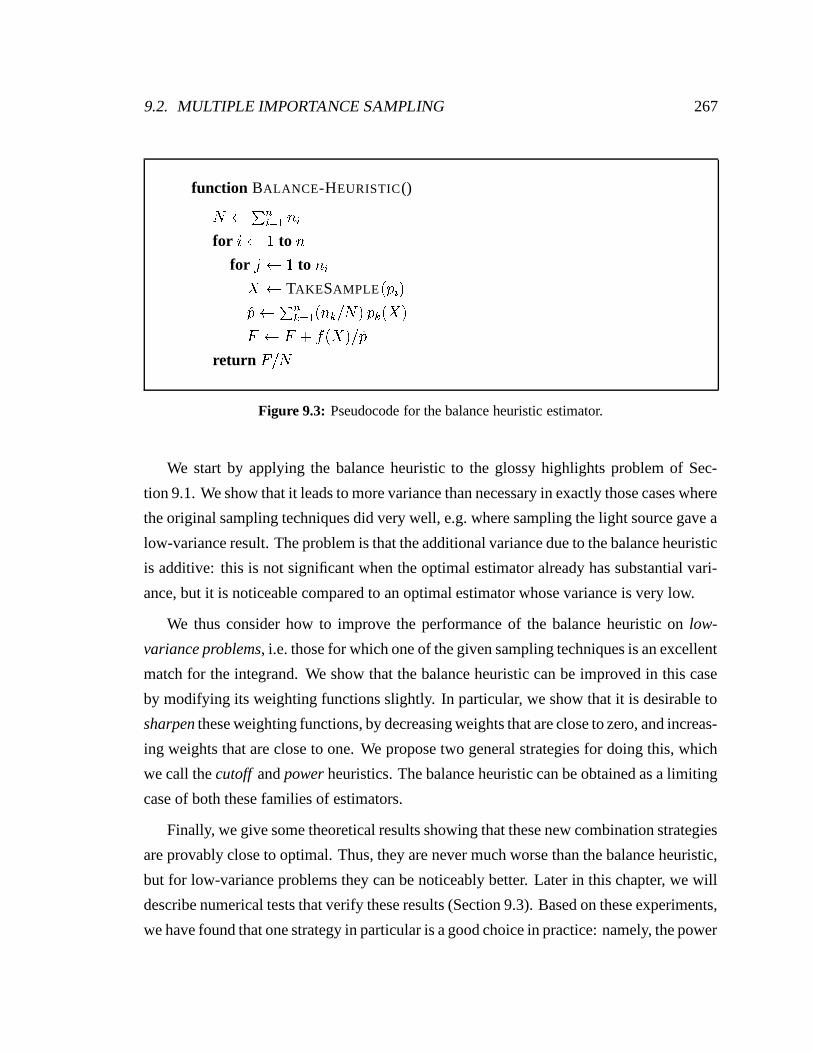
function BALANCE-HEURISTIC()
��� � � � � � �for ��� � to �
for ��� � to � ���� TAKESAMPLE � � � ����� � � � � � � � � � � � � � � ��
��� � ��� ��
return � �
Figure 9.3: Pseudocode for the balance heuristic estimator.
We start by applying the balance heuristic to the glossy highlights problem of Sec-
tion 9.1. We show that it leads to more variance than necessary in exactly those cases where
the original sampling techniques did very well, e.g. where sampling the light source gave a
low-variance result. The problem is that the additional variance due to the balance heuristic
is additive: this is not significant when the optimal estimator already has substantial vari-
ance, but it is noticeable compared to an optimal estimator whose variance is very low.
We thus consider how to improve the performance of the balance heuristic on low-
variance problems, i.e. those for which one of the given sampling techniques is an excellent
match for the integrand. We show that the balance heuristic can be improved in this case
by modifying its weighting functions slightly. In particular, we show that it is desirable to
sharpen these weighting functions, by decreasing weights that are close to zero, and increas-
ing weights that are close to one. We propose two general strategies for doing this, which
we call the cutoff and power heuristics. The balance heuristic can be obtained as a limiting
case of both these families of estimators.
Finally, we give some theoretical results showing that these new combination strategies
are provably close to optimal. Thus, they are never much worse than the balance heuristic,
but for low-variance problems they can be noticeably better. Later in this chapter, we will
describe numerical tests that verify these results (Section 9.3). Based on these experiments,
we have found that one strategy in particular is a good choice in practice: namely, the power
268 CHAPTER 9. MULTIPLE IMPORTANCE SAMPLING
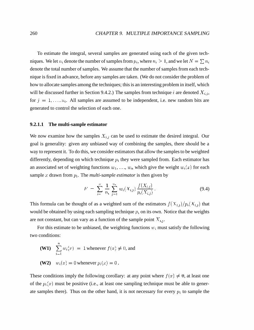
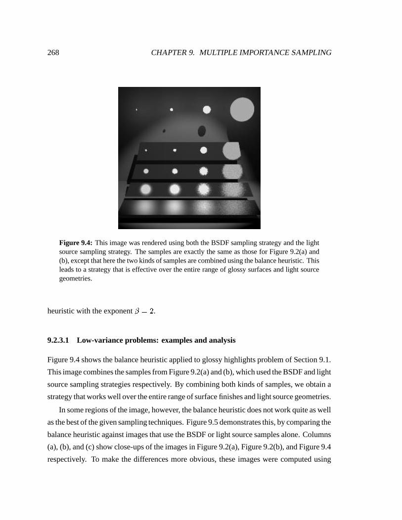
Figure 9.4: This image was rendered using both the BSDF sampling strategy and the lightsource sampling strategy. The samples are exactly the same as those for Figure 9.2(a) and(b), except that here the two kinds of samples are combined using the balance heuristic. Thisleads to a strategy that is effective over the entire range of glossy surfaces and light sourcegeometries.
heuristic with the exponent� ��� .
9.2.3.1 Low-variance problems: examples and analysis
Figure 9.4 shows the balance heuristic applied to glossy highlights problem of Section 9.1.
This image combines the samples from Figure 9.2(a) and (b), which used the BSDF and light
source sampling strategies respectively. By combining both kinds of samples, we obtain a
strategy that works well over the entire range of surface finishes and light source geometries.
In some regions of the image, however, the balance heuristic does not work quite as well
as the best of the given sampling techniques. Figure 9.5 demonstrates this, by comparing the
balance heuristic against images that use the BSDF or light source samples alone. Columns
(a), (b), and (c) show close-ups of the images in Figure 9.2(a), Figure 9.2(b), and Figure 9.4
respectively. To make the differences more obvious, these images were computed using
9.2. MULTIPLE IMPORTANCE SAMPLING 269
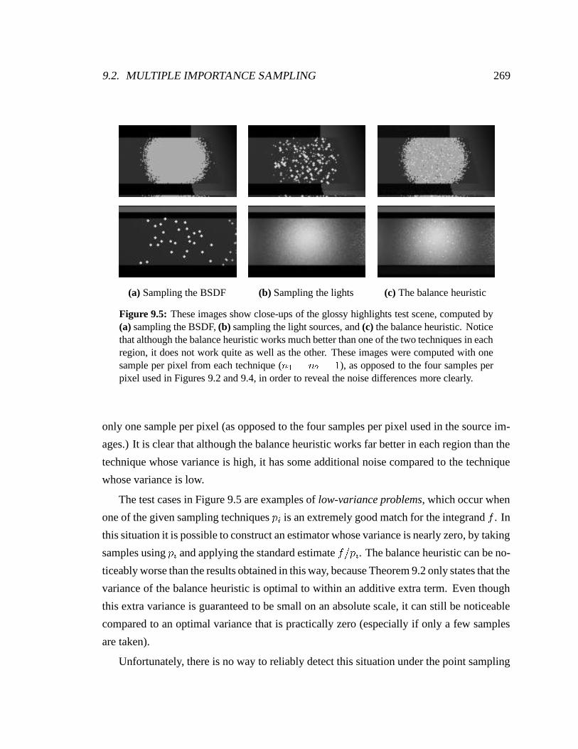
(a) Sampling the BSDF (b) Sampling the lights (c) The balance heuristic
Figure 9.5: These images show close-ups of the glossy highlights test scene, computed by(a) sampling the BSDF, (b) sampling the light sources, and (c) the balance heuristic. Noticethat although the balance heuristic works much better than one of the two techniques in eachregion, it does not work quite as well as the other. These images were computed with onesample per pixel from each technique ( � � � � � � �
), as opposed to the four samples perpixel used in Figures 9.2 and 9.4, in order to reveal the noise differences more clearly.
only one sample per pixel (as opposed to the four samples per pixel used in the source im-
ages.) It is clear that although the balance heuristic works far better in each region than the
technique whose variance is high, it has some additional noise compared to the technique
whose variance is low.
The test cases in Figure 9.5 are examples of low-variance problems, which occur when
one of the given sampling techniques � � is an extremely good match for the integrand�
. In
this situation it is possible to construct an estimator whose variance is nearly zero, by taking
samples using � � and applying the standard estimate�� � � . The balance heuristic can be no-
ticeably worse than the results obtained in this way, because Theorem 9.2 only states that the
variance of the balance heuristic is optimal to within an additive extra term. Even though
this extra variance is guaranteed to be small on an absolute scale, it can still be noticeable
compared to an optimal variance that is practically zero (especially if only a few samples
are taken).
Unfortunately, there is no way to reliably detect this situation under the point sampling
270 CHAPTER 9. MULTIPLE IMPORTANCE SAMPLING
0
f
p1
p2
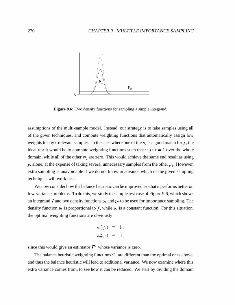
Figure 9.6: Two density functions for sampling a simple integrand.
assumptions of the multi-sample model. Instead, our strategy is to take samples using all
of the given techniques, and compute weighting functions that automatically assign low
weights to any irrelevant samples. In the case where one of the � � is a good match for�
, the
ideal result would be to compute weighting functions such that � � ��� � � � over the whole
domain, while all of the other � � are zero. This would achieve the same end result as using
� � alone, at the expense of taking several unnecessary samples from the other � � . However,
extra sampling is unavoidable if we do not know in advance which of the given sampling
techniques will work best.
We now consider how the balance heuristic can be improved, so that it performs better on
low-variance problems. To do this, we study the simple test case of Figure 9.6, which shows
an integrand�
and two density functions � � and � � to be used for importance sampling. The
density function � � is proportional to�
, while � � is a constant function. For this situation,
the optimal weighting functions are obviously
� �� � � ��� � � �� � � ��� �
since this would give an estimator �
whose variance is zero.
The balance heuristic weighting functions�� � are different than the optimal ones above,
and thus the balance heuristic will lead to additional variance. We now examine where this
extra variance comes from, to see how it can be reduced. We start by dividing the domain
9.2. MULTIPLE IMPORTANCE SAMPLING 271
0
f
p1
p2
B A B
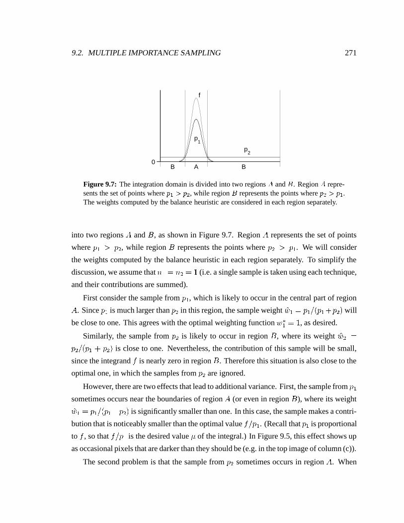
Figure 9.7: The integration domain is divided into two regions�
and � . Region�
repre-sents the set of points where � ��� � � , while region � represents the points where � � � � � .The weights computed by the balance heuristic are considered in each region separately.
into two regions and � , as shown in Figure 9.7. Region represents the set of points
where � ��� � � , while region � represents the points where � � � � � . We will consider
the weights computed by the balance heuristic in each region separately. To simplify the
discussion, we assume that � � � � � � � (i.e. a single sample is taken using each technique,
and their contributions are summed).
First consider the sample from � � , which is likely to occur in the central part of region
. Since � � is much larger than � � in this region, the sample weight�� � � � � � � � � � � � � will
be close to one. This agrees with the optimal weighting function � �� � � , as desired.
Similarly, the sample from � � is likely to occur in region � , where its weight�� � �
� � � � � � � � � � is close to one. Nevertheless, the contribution of this sample will be small,
since the integrand�
is nearly zero in region � . Therefore this situation is also close to the
optimal one, in which the samples from � � are ignored.
However, there are two effects that lead to additional variance. First, the sample from � �sometimes occurs near the boundaries of region (or even in region � ), where its weight�� � � � � � � � � � � � � is significantly smaller than one. In this case, the sample makes a contri-
bution that is noticeably smaller than the optimal value�� � � . (Recall that � � is proportional
to�
, so that�� � � is the desired value � of the integral.) In Figure 9.5, this effect shows up
as occasional pixels that are darker than they should be (e.g. in the top image of column (c)).
The second problem is that the sample from � � sometimes occurs in region . When

272 CHAPTER 9. MULTIPLE IMPORTANCE SAMPLING
this happens, its weight�� � � � � � � � � � � � � is small. However, the contribution made by
this sample is �� � �� � � � �� � � � �
�� �
� �� � � � �
which is approximately equal to�� � � � � in this region. Since it is likely that the sample
from � � also lies in region (contributing another � toward the estimate), this leads to a total
estimate of approximately � � . In Figure 9.5(c), this effect shows up as occasional pixels that
are approximately twice as bright as their neighbors.4
Thus, the additional noise of the balance heuristic can be attributed to two problems.
First, some of the samples from � � have weights that are significantly smaller than one: this
happens near the boundary of region , where � � and � � have comparable magnitude. (Very
few of these samples will occur in the region where � ��� � � , simply because � � is very small
there.) The second problem is that some samples from � � make contributions of noticeable
size (i.e. a significant fraction of � ). Most of these samples have small weights, because
they occur in region where � � � � � . Some samples will also occur in the region where
� � and � � have comparable magnitude; however, the samples where � ��� � � do not cause
any problems, since the sample contribution�� � � � � � � � is negligible there.
9.2.3.2 Better strategies for low-variance problems
We now present two families of combination strategies that have better performance on
low-variance problems. These strategies are variations of the balance heuristic, where the
weighting functions have been sharpened by making large weights closer to one and small
weights closer to zero. This idea is effective at reducing both sources of variance described
above.
The basic observation is that most samples from � � occur in region , where � � � � � .We would like all of these samples to have the optimal weight � �� � � . Since the balance
heuristic already assigns these samples a weight�� � � � � � � � � � � � � that is greater than � � � ,
we can get closer to the optimal weighting functions by applying the sharpening strategy
mentioned above. For example, one way to do this would be to set � � � � (and � � ��� )4Note that this situation is entirely different than the “spikes” of Figure 9.5(a) and (b), which are caused
by sample contributions that are hundreds of times larger than the desired mean value.
9.2. MULTIPLE IMPORTANCE SAMPLING 273
whenever�� � � � � � .
Similarly, this idea can reduce the variance caused by samples from � � in region . The
optimal weight for these samples is � �� � � , while the balance heuristic assigns them a
weight�� � � � � � , so that sharpening the weighting functions is once again an effective
strategy.5
We now describe two different combination strategies that implement this sharpening
idea, called the cutoff heuristic and the power heuristic. Each of these is actually a family
of strategies, controlled by an additional parameter. For convenience in describing them,
we will drop the � argument on the functions � � and � � , and define a new symbol � � as the
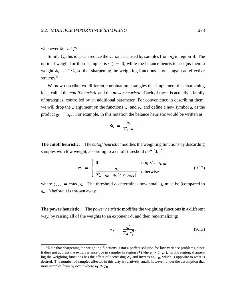
product � � � � � � � . For example, in this notation the balance heuristic would be written as�� � � � �� � � � �
The cutoff heuristic. The cutoff heuristic modifies the weighting functions by discarding
samples with low weight, according to a cutoff threshold � � � � � � :� � �
���� ���� if � � � ��������
� �� �� � � � � � � ��������� otherwise(9.12)
where ������ � ����� � � � . The threshold � determines how small � � must be (compared to
������ ) before it is thrown away.
The power heuristic. The power heuristic modifies the weighting functions in a different
way, by raising all of the weights to an exponent�
, and then renormalizing:
� � � ����� � � �� � (9.13)
5Note that sharpening the weighting functions is not a perfect solution for low-variance problems, sinceit does not address the extra variance due to samples in region � (where ����� ��� ). In this region, sharpen-ing the weighting functions has the effect of decreasing � and increasing � , which is opposite to what isdesired. The number of samples affected in this way is relatively small, however, under the assumption thatmost samples from � � occur where � ��� � � .
274 CHAPTER 9. MULTIPLE IMPORTANCE SAMPLING
We have found the exponent� � � to be a reasonable value. With this choice, the sample
contribution � � ��� � � � � � � � is proportional to � � , so that it decreases gradually as � � becomes
smaller relative to the other � � . (Compare this with the balance heuristic, where a sample at
a given point � always makes the same contribution, no matter which sampling technique
generated it.)
Notice that the balance heuristic can be obtained as a limiting case of both strategies
(when � � � or� � � ). These two strategies also share another limiting case, obtained by
setting � � � or� ��� . This special case is called the maximum heuristic:
The maximum heuristic. The maximum heuristic partitions the domain into � regions,
according to which function � � is largest at each point � :
� � ��� � � if � � � ������� otherwise �
(9.14)
In other words, samples from � � are used to estimate the integral only in the region � � where
� � � � . The maximum heuristic does not work as well as the other strategies in practice; in-
tuitively, this is because too many samples are thrown away. However, it gives some insight
into the other combination strategies, and has an elegant structure.
9.2.3.3 Variance bounds
The advantage of these strategies is reduced variance when one of the � � is a good match
for�
. Their performance is otherwise similar to the balance heuristic; it is possible to show
they are never much worse. In particular, we have the following worst-case bounds:
Theorem 9.3. Let�
, � � , and � � be given, for � � � � � � � . Let
be any unbiased estimator
of the form (9.4), and let � be one of the estimators described above. Then the variance of � satisfies a bound of the form
� � � ��� � � � �� � � ���� � � � � � �� � � � � �
where the constant � is given by the following table:
9.2. MULTIPLE IMPORTANCE SAMPLING 275
Cutoff heuristic (with threshold � ) � � � � � � � � � �Power heuristic (with exponent
�) � � � � � � � � � ��� � � � � � � � � � � � � � � � ��� ��� �
Power heuristic (with exponent� � � ) � � � � � � � � � ��� � �
In particular, these bounds hold when � is compared against the unknown, optimal es-
timator �
. A proof of this theorem in given in Appendix 9.A. However, the true test of
these strategies is how they perform on practical problems; measurements along these lines
are presented in Section 9.3.1.
9.2.4 The one-sample model
We conclude by considering a different model for how the samples are taken and combined,
called the one-sample model. Under this model, the integral is estimated by choosing one
of the � sampling techniques at random, and then taking a single sample from it. Again
we consider how to minimize variance by weighting the samples, and we show that for this
model the balance heuristic is optimal: no other combination technique has smaller vari-
ance.
Let � � , � ��� , � be the density functions for the � given sampling techniques. To gen-
erate a sample, one of the density functions � � is chosen at random according to a given
set of probabilities � � , � ��� , � (which sum to one). A single sample is then taken from the
chosen technique. This sampling model is often used in graphics: for example, it describes
algorithms such as path tracing, where sampling the BSDF may require a random choice
between different techniques for the diffuse, glossy, and specular components.
As before, we consider a family of unbiased estimators for the given integral� � � ��� ����� � � � , where each estimator is represented by a set of weighting functions � � ,� � � , � . The process of choosing a sampling technique, taking a sample, and computing a
weighted estimate is then expressed by the one-sample estimator
� ��� � �� ��� �� �
� � �� � �� � (9.15)
where � � � � ��� � is a random variable distributed according to the probabilities � � , and
276 CHAPTER 9. MULTIPLE IMPORTANCE SAMPLING
�� is a sample from the corresponding technique � � . This estimator is unbiased under the
same conditions on the � � discussed in Section 9.2.1.
We now consider how to choose the weighting functions � � , to minimize the variance
of the resulting estimator. We can show that for this model, the balance heuristic is optimal:
Theorem 9.4. Let�
, � � , and � � be given, for � � � ��� � � . Let
be any unbiased estimator
of the form (9.15), and let�
be the corresponding estimator that uses the balance heuristic
weighting functions (9.8). Then� � ��� � � � �� �
(A proof is given in Appendix 9.A.) Thus, for this sampling model the improved com-
bination strategies of Section 9.2.3 are unnecessary.
9.3 Results
In this section, we show how multiple importance sampling can be applied to two impor-
tant application areas: distribution ray tracing (in particular, the glossy highlights problem
from Section 9.1), and the final gather pass of certain light transport algorithms. (In the next
chapter we will describe a more advanced example of our techniques, namely bidirectional
path tracing.)
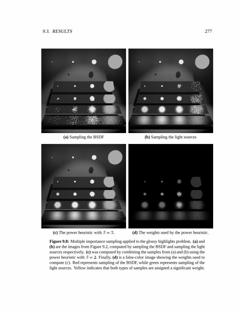
9.3.1 The glossy highlights problem
Our first test is the computation of glossy highlights from area light sources (previously de-
scribed in Section 9.1). As can be seen in Figure 9.8(a) and (b), sampling the BSDF works
well for sharp reflections of large light sources, while sampling the light source works well
for fuzzy reflections of small light sources. In Figure 9.8(c), we have used the power heuris-
tic with� � � to combine both kinds of samples. This method works very well for all light
source/BSDF combinations. Figure 9.8(d) is a visualization of the weighting functions that
were used to compute this image.
To compare the various combination strategies (the balance, cutoff, power, and maxi-
mum heuristics), we have measured the variance numerically as a function of the surface
9.3. RESULTS 277
(a) Sampling the BSDF (b) Sampling the light sources
(c) The power heuristic with� ��� . (d) The weights used by the power heuristic.
Figure 9.8: Multiple importance sampling applied to the glossy highlights problem. (a) and(b) are the images from Figure 9.2, computed by sampling the BSDF and sampling the lightsources respectively. (c) was computed by combining the samples from (a) and (b) using thepower heuristic with
� ��� . Finally, (d) is a false-color image showing the weights used tocompute (c). Red represents sampling of the BSDF, while green represents sampling of thelight sources. Yellow indicates that both types of samples are assigned a significant weight.

278 CHAPTER 9. MULTIPLE IMPORTANCE SAMPLING
glossy surface
lightspherical
source
Figure 9.9: A scale diagram of the scene model used to measure the variance of the glossyhighlights calculation. The glossy surface is illuminated by a single spherical light source,so that a blurred reflection of the light source is visible from the camera position. Variancewas measured by taking 100,000 samples along the viewing ray shown, which intersects thecenter of the blurred reflection at an angle of 45 degrees. This calculation was repeated forapproximately 100 different values of the surface roughness parameter
�(which controls
how sharp or fuzzy the reflections are), in order to measure the variance as a function ofsurface roughness. The light source occupies a solid angle of 0.063 radians.
roughness parameter � . Figure 9.9 shows the test setup, and the results are summarized in
Figure 9.10. Three curves are shown in each graph: two of them correspond to the BSDF
and light source sampling techniques, while the third corresponds to the combination strat-
egy being tested (i.e. the balance, cutoff, power, or maximum heuristic). Each graph plots
the relative error � � � as a function of � , where � is the standard deviation of a single sample,
and � is the mean.
Notice that all four combination strategies yield a variance that is close to the minimum
of the two other curves (on an absolute scale). This is in accordance with Theorem 9.2,
which guarantees that the variance � � of the balance heuristic is within � � � � of the vari-
ance obtained when either of the given sampling techniques is used on its own. The plots
in Figure 9.10(a) are well within this bound.
At the extremes of the roughness axis there are significant differences among the var-
ious combination strategies. As expected, the balance heuristic (a) performs worst at the
extremes, since the other strategies were specifically designed to have better performance
in this case (i.e. the case when one of the given sampling techniques is an excellent match
for the integrand). The power heuristic (c) with� � � works especially well over the entire
range of roughness values.
9.3. RESULTS 279
10−6
10−4
10−2
100
0
0.5
1
1.5
2
sample light sample BSDF
balanceheuristic
surface roughness r
rela
tive
erro
r σ
/µ
10−6
10−4
10−2
100
0
0.5
1
1.5
2
sample light sample BSDF
cutoffheuristic
surface roughness r
rela
tive
erro
r σ
/µ
(a) The balance heuristic. (b) The cutoff heuristic ( � � ��� � ).
10−6
10−4
10−2
100
0
0.5
1
1.5
2
sample light sample BSDF
powerheuristic
surface roughness r
rela
tive
erro
r σ
/µ
10−6
10−4
10−2
100
0
0.5
1
1.5
2
sample light sample BSDF
maximumheuristic
surface roughness r
rela
tive
erro
r σ
/µ
(c) The power heuristic (� ��� ). (d) The maximum heuristic.
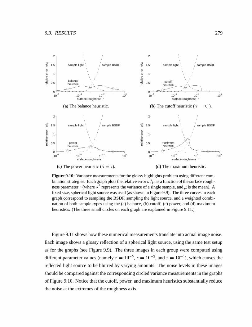
Figure 9.10: Variance measurements for the glossy highlights problem using different com-bination strategies. Each graph plots the relative error �
�� as a function of the surface rough-
ness parameter�
(where ��
represents the variance of a single sample, and � is the mean). Afixed size, spherical light source was used (as shown in Figure 9.9). The three curves in eachgraph correspond to sampling the BSDF, sampling the light source, and a weighted combi-nation of both sample types using the (a) balance, (b) cutoff, (c) power, and (d) maximumheuristics. (The three small circles on each graph are explained in Figure 9.11.)
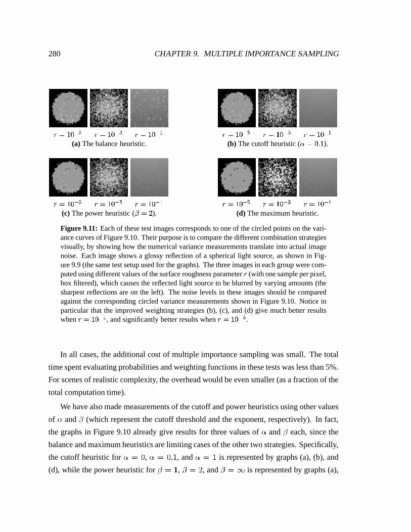
Figure 9.11 shows how these numerical measurements translate into actual image noise.
Each image shows a glossy reflection of a spherical light source, using the same test setup
as for the graphs (see Figure 9.9). The three images in each group were computed using
different parameter values (namely � � � � ��� , � � � � � �
, and � � � � � � ), which causes the
reflected light source to be blurred by varying amounts. The noise levels in these images
should be compared against the corresponding circled variance measurements in the graphs
of Figure 9.10. Notice that the cutoff, power, and maximum heuristics substantially reduce
the noise at the extremes of the roughness axis.
280 CHAPTER 9. MULTIPLE IMPORTANCE SAMPLING
� � � � ��� � � � � � �� � � � � � � � � � ��� � � � � � �
� � � � � �(a) The balance heuristic. (b) The cutoff heuristic ( � � ��� � ).
� � � � ��� � � � � � �� � � � � � � � � � ��� � � � � � �
� � � � � �(c) The power heuristic (
� ��� ). (d) The maximum heuristic.
Figure 9.11: Each of these test images corresponds to one of the circled points on the vari-ance curves of Figure 9.10. Their purpose is to compare the different combination strategiesvisually, by showing how the numerical variance measurements translate into actual imagenoise. Each image shows a glossy reflection of a spherical light source, as shown in Fig-ure 9.9 (the same test setup used for the graphs). The three images in each group were com-puted using different values of the surface roughness parameter
�(with one sample per pixel,
box filtered), which causes the reflected light source to be blurred by varying amounts (thesharpest reflections are on the left). The noise levels in these images should be comparedagainst the corresponding circled variance measurements shown in Figure 9.10. Notice inparticular that the improved weighting strategies (b), (c), and (d) give much better resultswhen
� � � � � � , and significantly better results when� � � � ��� .
In all cases, the additional cost of multiple importance sampling was small. The total
time spent evaluating probabilities and weighting functions in these tests was less than 5%.
For scenes of realistic complexity, the overhead would be even smaller (as a fraction of the
total computation time).
We have also made measurements of the cutoff and power heuristics using other values
of � and�
(which represent the cutoff threshold and the exponent, respectively). In fact,
the graphs in Figure 9.10 already give results for three values of � and�
each, since the
balance and maximum heuristics are limiting cases of the other two strategies. Specifically,
the cutoff heuristic for � � � , � � � � � , and � � � is represented by graphs (a), (b), and
(d), while the power heuristic for� � � , � � � , and
� � � is represented by graphs (a),

9.3. RESULTS 281
(c), and (d). The graphs we have obtained at other parameter values are not significantly
different than what would be obtained by interpolating these results.
Related work. Shirley & Wang [1992] have also compared BRDF and light source sam-
pling techniques for the glossy highlights problem. They analyze a specific Phong-like
BRDF and a specific light source sampling method, and derive an expression for when to
switch from one to the other (as a function of the Phong exponent, and the solid angle oc-
cupied by the light source). Their methods work well, but they apply only to this particular
BSDF and sampling technique. In contrast, our methods work for arbitrary BSDF’s and
sampling techniques, and can combine samples from any number of techniques.
9.3.2 The final gather problem
In this section we consider a simple test case motivated by multi-pass light transport algo-
rithms. These algorithms typically compute an approximate solution using the finite ele-
ment method, followed by one or more ray tracing passes to replace parts of the solution
that are poorly approximated or missing. For example, some radiosity algorithms use a lo-
cal pass or final gather to recompute the basis function coefficients more accurately.
We examine a variation called per-pixel final gather. The idea is to compute an approxi-
mate radiosity solution, and then use it to illuminate the visible surfaces during a ray tracing
pass [Rushmeier 1988, Chen et al. 1991]. Essentially, this type of final gather is equivalent
to ray tracing with many area light sources (one for each patch, or one for each link in a hi-
erarchical solution). That is, we would like to evaluate the scattering equation (9.2) where
��� is given by the initial radiosity solution.
As with the glossy highlights example, there are two common sampling techniques. The
brightest patches are typically reclassified as “light sources” [Chen et al. 1991], and are sam-
pled using direct lighting techniques. For example, this might consist of choosing one sam-
ple for each light source patch, distributed according to the emitted power per unit area.
The remaining patches are handling by sampling the BSDF at the point intersected by the
viewing ray, and casting rays out into the scene. If any ray hits a light source patch, the con-
tribution of that ray is set to zero (to avoid counting the light source patches twice). Within

282 CHAPTER 9. MULTIPLE IMPORTANCE SAMPLING
(a) (b) (c)
Figure 9.12: A simple test scene consisting of one area light source (i.e. a bright patch,in the radiosity context), and an adjacent diffuse surface. The images were computed by(a) sampling the light source according to emitted power, using � � ��� samples per pixel,(b) sampling the BSDF with respect to the projected solid angle measure, using � � ���samples per pixel, and (c) a weighted combination of samples from (a) and (b) using thepower heuristic with
� ��� .
our framework for combining sampling techniques, this is clearly a partitioning of the inte-
gration domain into two regions.
Given some classification of patches into light sources and non-light sources, we con-
sider alternative ways of combining the two types of samples. To test our combination
strategies, we used the extremely simple test scene of Figure 9.12, which consists of a sin-
gle area light source and an adjacent diffuse surface. Image (a) was computed by sampling
the light source according to emitted power, while image (b) was computed by sampling the
BSDF and casting rays out into the scene. Twice as many samples were taken in image (b)
than (a); in practice this ratio would be substantially higher (i.e. the number of directional
samples, compared to the number of samples for any one light source).
Notice that the sampling technique in Figure 9.12(a) does not work well for points near
the light source, since this technique does not take into account the � � � � distance term of the
scattering equation (9.2). On the other hand Figure 9.12(b) does not work well for points far
away from the light source, where the light subtends a small solid angle. In Figure 9.12(c),
the power heuristic is used to combine samples from (a) and (b). As expected, this method
performs well at all distances. Although (c) uses more samples (the sum of (a) and (b)), this
still is a valid comparison with the partitioning approach described above (which also uses
9.4. DISCUSSION 283
0 0.2 0.4 0.6 0.8 10
1
2
3
4
5
(a)
(b)
(c)
distance from light source
rela
tive
erro
r σ
/µ
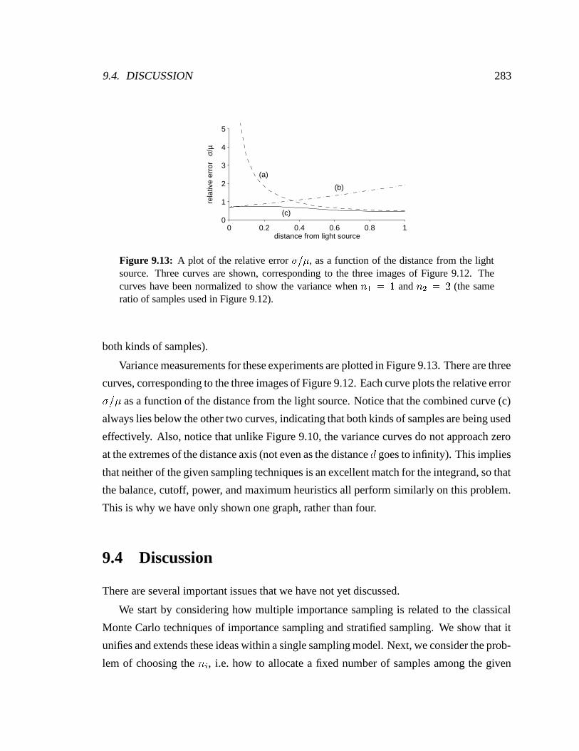
Figure 9.13: A plot of the relative error ��� , as a function of the distance from the light
source. Three curves are shown, corresponding to the three images of Figure 9.12. Thecurves have been normalized to show the variance when � ��� �
and � � � � (the sameratio of samples used in Figure 9.12).
both kinds of samples).
Variance measurements for these experiments are plotted in Figure 9.13. There are three
curves, corresponding to the three images of Figure 9.12. Each curve plots the relative error
� � � as a function of the distance from the light source. Notice that the combined curve (c)
always lies below the other two curves, indicating that both kinds of samples are being used
effectively. Also, notice that unlike Figure 9.10, the variance curves do not approach zero
at the extremes of the distance axis (not even as the distance � goes to infinity). This implies
that neither of the given sampling techniques is an excellent match for the integrand, so that
the balance, cutoff, power, and maximum heuristics all perform similarly on this problem.
This is why we have only shown one graph, rather than four.
9.4 Discussion
There are several important issues that we have not yet discussed.
We start by considering how multiple importance sampling is related to the classical
Monte Carlo techniques of importance sampling and stratified sampling. We show that it
unifies and extends these ideas within a single sampling model. Next, we consider the prob-
lem of choosing the � � , i.e. how to allocate a fixed number of samples among the given

284 CHAPTER 9. MULTIPLE IMPORTANCE SAMPLING
sampling techniques. We argue that this decision is not nearly as important as choosing the
weighting functions appropriately. Finally, we discuss some special issues that arise in di-
rect lighting problems.
9.4.1 Relationship to classical Monte Carlo techniques
Multiple importance sampling can be viewed as a generalization of both importance sam-
pling and stratified sampling. It extends importance sampling to the case where more than
one sampling technique is used, while it extends stratified sampling to the case where the
strata are allowed to overlap each other. From the latter point of view, multiple importance
sampling consists of taking one or more samples in each of � given regions � � . These re-
gions do not need to be disjoint; the only requirement is that their union must cover the
portion of the domain where�
is non-zero.
This generalization of stratified sampling is useful, especially when the integrand is a
sum of several quantities. A good example in graphics is the BSDF, which is often written
as a sum of diffuse, glossy, and specular components (for reflection and/or transmission).
The process of taking one or more samples from each component is essentially a form of
stratified sampling, where the strata overlap.
When stratified sampling is generalized in this way, however, there is more than one
way to compute an unbiased estimate of the integral (since when two strata overlap, sam-
ples from either or both strata can be used). To address this, multiple importance sampling
assigns an explicit representation to each possible unbiased estimator (as a set of weighting
functions � � ). Furthermore it provides a reasonable way to select one of these estimators,
by showing that certain estimators perform well compared to all the rest.
9.4.2 Allocation of samples among the techniques
In this section, we consider how to choose the number of samples that are taken using each
technique � � . We show that this decision is not as important as it might seem at first: no
strategy is that much better than that of simply setting all the � � equal.
To see this, suppose that a total of � samples will be taken, and that these samples must
be allocated among the � sampling techniques. Let
be an estimator that allocates these
9.4. DISCUSSION 285
samples in any way desired (provided that � � � � � � ), and uses any weighting functions
desired (provided that
is unbiased). On the other hand, let�
be the estimator that takes
an equal number of samples from each � � , and combines them using the balance heuristic.
Then it is straightforward to show that
� � ����� � � � �� � � � �� � �
where as usual, � � ��� ��is the quantity to be estimated (see Theorem 9.5 in Appendix 9.A
for a proof).
According to this result, changing the � � can improve the variance by at most a factor
of � , plus a small additive term. In contrast, a poor choice of the � � can increase variance
by an arbitrary amount. Thus, the sample allocation is not as important as choosing a good
combination strategy.
Furthermore, the sample allocation is often controlled by other factors, so that the opti-
mal sample allocation is irrelevant. For example, consider the glossy highlights problem. In
a distribution ray tracer, the samples used to estimate the glossy highlights are also used for
other purposes: e.g. the light source samples are used to estimate the diffuse shading of the
surface, while the BSDF samples are used to compute glossy reflections of ordinary, non-
light-source objects. Often these other purposes will dictate the number of samples taken, so
that the sample allocation for the glossy highlights calculation cannot be chosen arbitrarily.
On the other hand, by computing an appropriate weighted combination of the samples that
need to be taken anyway, we can reduce the variance of the highlight calculation essentially
for free.
Similarly, the sample allocation is also constrained in bidirectional path tracing. In this
case, it is for efficiency reasons: it is more efficient to take one sample from all the tech-
niques at once, rather than taking different numbers of samples using each strategy. (This
will be discussed further in Chapter 10.)
9.4.3 Issues for direct lighting problems
The glossy highlights and final gather test cases are both examples of direct lighting prob-
lems. They differ only in the terms of the scattering equation that cause high variance: in

286 CHAPTER 9. MULTIPLE IMPORTANCE SAMPLING
the case of glossy highlights, it was the BSDF and the emission function � � , while for the
final gather problem it was the � � � � distance factor.
Although there are more sophisticated techniques for direct lighting that take into ac-
count more factors of the scattering equation [Shirley et al. 1996], it is still useful to combine
several kinds of samples. There are several reasons for this. First, sophisticated sampling
strategies are generally designed for a specific light source geometry (e.g. the light source
must be a triangle or a sphere). Second, they are often expensive: for example, taking a sam-
ple may involve numerical inversion of a function. Third, none of these strategies is perfect:
there are always some factors of the scattering equation that are not included in the approx-
imation (e.g. virtually all direct lighting strategies do not consider the BSDF or visibility
factors). Thus, in parts of the scene where these unconsidered factors are dominant, it can
be more efficient to use a simpler technique such as sampling the BSDF. Thus, combining
samples from two or more techniques can make direct lighting calculations more robust.
9.5 Conclusions and recommendations
As we have shown, multiple importance sampling can substantially reduce the variance
of Monte Carlo rendering calculations. These techniques are practical, and the additional
cost is small — less than 5% of the time in our tests was spent evaluating probabilities and
weighting functions. There are also good theoretical reasons to use these methods, since we
have shown strong bounds on their performance relative to all other combination strategies.
For most Monte Carlo problems, the balance heuristic is an excellent choice for a com-
bination strategy: it has the best theoretical bounds, and is the simplest to implement. The
additional variance term of � � � � ��� � � � � � � � � � � is not an issue for integration problems
of reasonable complexity, because it is unlikely that any of the given density functions � �will be an excellent match for
�. Under these circumstances, even the optimal combination �
has considerable variance, so that the maximum improvement that can be obtained by
using some other strategy instead of the balance heuristic is a small fraction of the total.
On the other hand, if it is possible that the given integral is a low-variance problem (i.e.
one of the � � is good match for�
), then the power heuristic with� � � is an excellent choice.
It performs similarly to the balance heuristic overall, but gives better results on low-variance

9.5. CONCLUSIONS AND RECOMMENDATIONS 287
problems (which is exactly the case where better performance is most noticeable). Direct
lighting calculations are a good example of where this optimization is useful.
In effect, multiple importance sampling provides a new viewpoint on Monte Carlo inte-
gration. Unlike ordinary importance sampling, where the goal is to find a single “perfect”
sampling technique, here the goal is to find a set of techniques that cover the important fea-
tures of the integrand. It does not matter if there are a few bad sampling techniques as well
— some effort will be wasted in sampling them, but the results will not be significantly af-
fected. Thus, multiple importance sampling gives a recipe for making Monte Carlo software
more reliable: whenever there is some situation that is not handled well, then we can sim-
ply add another sampling technique designed for that situation alone. We believe that there
are many applications that could benefit from this approach, both in computer graphics and
elsewhere.
288 CHAPTER 9. MULTIPLE IMPORTANCE SAMPLING
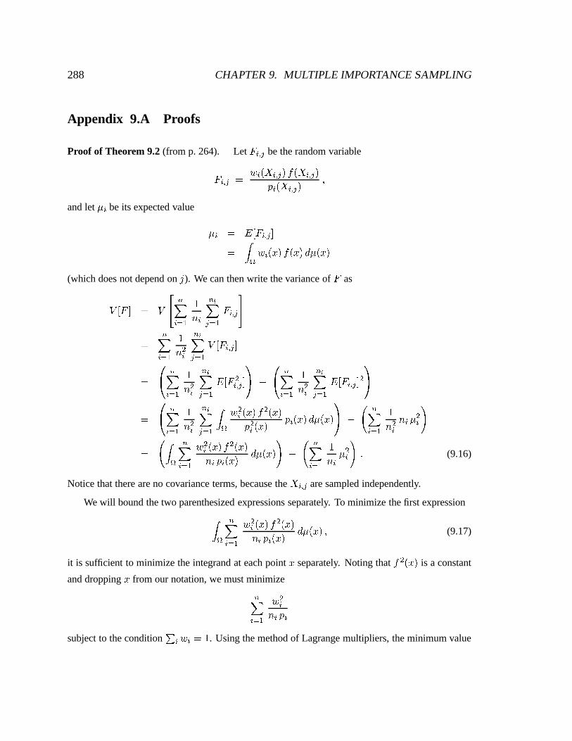
Appendix 9.A Proofs
Proof of Theorem 9.2 (from p. 264). Let � � � � be the random variable
� � � � � � � ��� � � � � ��� � � � � ����� � � �
and let � � be its expected value
� � � ��� � � � ���� �
� � � � � � �� � � (which does not depend on ). We can then write the variance of � as
� � � � � ���� ��� �
�� � � � � � � � ����
� � � �
�� ��
� � � �
� � � � � ���� ��
��� ��� ��
� � � ��� � �� � � ���� � ��
��� ��� ��
� � � � ��� � � � ��� � ��
� �� ��� �
�� ��
� � �
��� �� � � � � ���
� � �
��� � � �� � �
��� ��� �� � � �
��
� � � � ��� �
� �� � � � � � � � � � � � � � � ��� �
�� � �
�� � (9.16)
Notice that there are no covariance terms, because the�� � � are sampled independently.
We will bound the two parenthesized expressions separately. To minimize the first expression����� �
� �� � � � � � � � � � � � � � (9.17)
it is sufficient to minimize the integrand at each point
separately. Noting that� � � is a constant
and dropping
from our notation, we must minimize
��� �
� ��� � � �
subject to the condition � � � � � �. Using the method of Lagrange multipliers, the minimum value
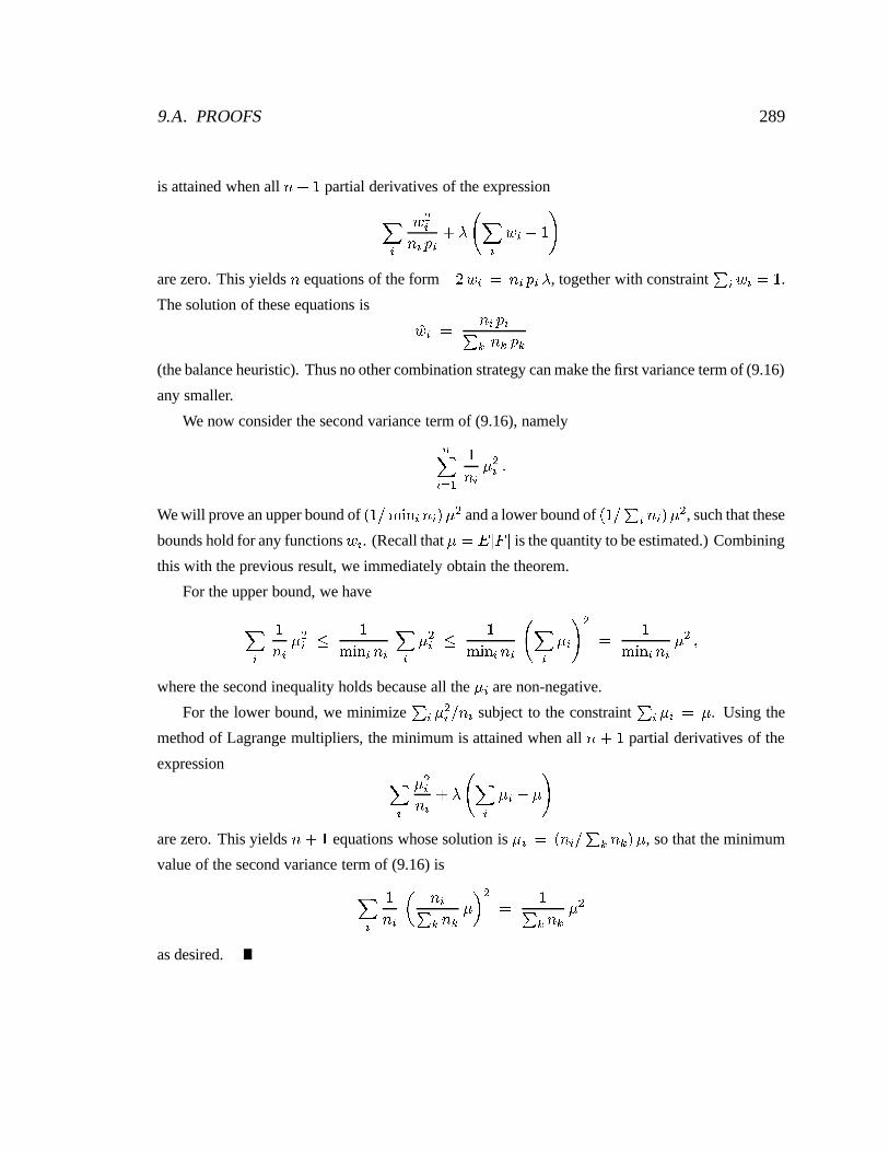
9.A. PROOFS 289
is attained when all ��� �partial derivatives of the expression
�
� ��� � � � ��� � � � � � �
are zero. This yields � equations of the form � � � � � � � � � � , together with constraint � � � � � �.
The solution of these equations is �� � � � � � �� � � � � �(the balance heuristic). Thus no other combination strategy can make the first variance term of (9.16)
any smaller.
We now consider the second variance term of (9.16), namely
��� �
�� � �
�� �
We will prove an upper bound of����������
� � � � � and a lower bound of����� � � � � � � , such that these
bounds hold for any functions � � . (Recall that � � ��� � � is the quantity to be estimated.) Combining
this with the previous result, we immediately obtain the theorem.
For the upper bound, we have
�
�� � �
�� �
������ � �
�
��� �
������ � �
� �
� � � ������ � � �
� �where the second inequality holds because all the � � are non-negative.
For the lower bound, we minimize � � � ��� � � subject to the constraint � � � � � � . Using the
method of Lagrange multipliers, the minimum is attained when all ��� �partial derivatives of the
expression �
� ��� � ��� � � � � � �
are zero. This yields ��� �equations whose solution is � � � � � � � � � � � � , so that the minimum
value of the second variance term of (9.16) is
�
�� � � �� � � � ���
��
�� � � � �
�
as desired.
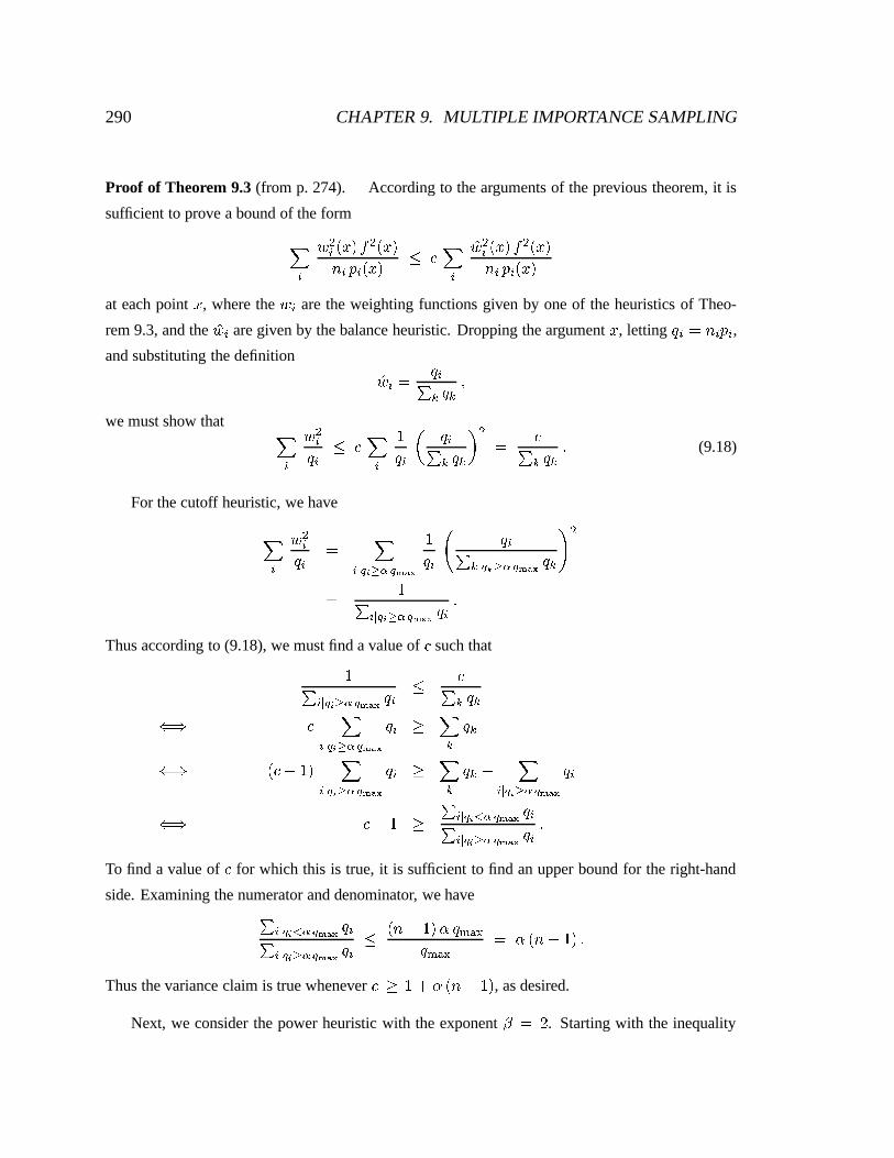
290 CHAPTER 9. MULTIPLE IMPORTANCE SAMPLING
Proof of Theorem 9.3 (from p. 274). According to the arguments of the previous theorem, it is
sufficient to prove a bound of the form
�
� �� � � � � � � � � � ����
�� �� � � � � � � � � � at each point
, where the � � are the weighting functions given by one of the heuristics of Theo-
rem 9.3, and the�� � are given by the balance heuristic. Dropping the argument
, letting � � � � � � � ,
and substituting the definition �� � � � �� � � � �we must show that
�
� ��� � ���
�
�� � � �� � � �
� � � �� � � � � (9.18)
For the cutoff heuristic, we have
�
� ��� � �
��� � ��� �� ����� �� � �� � � ��� �� �� ��� � � �
��
� ��� � ��� �� ��� � � �
Thus according to (9.18), we must find a value of � such that�� ��� � ��� �� ��� � � � �� � � ��
��� � ��� � ��� �
���� � �
� �
�� �
� ��� � ��� � ��� �
���� � �
� � � ��� � ��� � ��� �
�
� ��
��� � � ��� � ��� � ��� � �� ��� � ��� � ��� � � �
To find a value of � for which this is true, it is sufficient to find an upper bound for the right-hand
side. Examining the numerator and denominator, we have
� ��� � ��� �� ��� � �� ��� � ��� �� ��� � � �� � �
� ��� ����
� ���� � �
� � �� �
Thus the variance claim is true whenever � �� � �
� � �� , as desired.
Next, we consider the power heuristic with the exponent� � � . Starting with the inequality

9.A. PROOFS 291
(9.18), we have�
� ��� � �
�
�� �� �
��
� � � �� � � � � � ��� � � � ���� � � (9.19)
Thus we must find a value of � such that
� � � ��� � � � �� � � � �� � � �� � � � � � � � � �� �� � � �
� � � � �� � � � (9.20)
Notice that this inequality is unchanged if all the � � are scaled by a constant factor. Thus without loss
of generality we can assume that ���� �
�� � � (9.21)
so that our goal reduces to finding a value of � such that
� � � � � � �� � � � � � � �� � �
We proceed as before, by finding an upper bound for the right-hand side. Without loss of generality,
let � � be the largest of the � � . Observing that� � � � �� � � � � � � �� � � �����
� � � � ��� �it is sufficient to find an upper bound for � � . According to (9.21), we have
��� � ��� �
��� � � � � ��� �
Letting � denote the quantity on the right-hand side, we have � � ����� � � � �
� , since the maximum
value of � � � ��� is attained when � � � ���
� . Thus using the quadratic formula, we have
�� � � � � � ����� �
� � ��
� �� � � ������ ��� ��� � � � � � � ����� �
� � ��
� ������ ��� � � �
Thus, the original inequality (9.18) is true for any value of � larger than this.
For an exponent in the range� � � ��� , the argument is similar. We find that
�
� ��� � � � � � � � � � �� � � � � � �� �
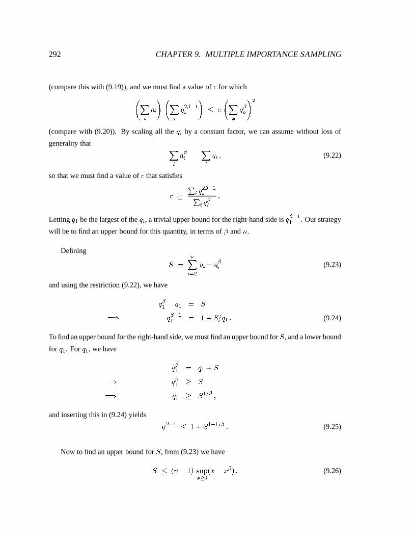
292 CHAPTER 9. MULTIPLE IMPORTANCE SAMPLING
(compare this with (9.19)), and we must find a value of � for which� �
� � � �
�� � � �� ���
� �
� �� �(compare with (9.20)). By scaling all the � � by a constant factor, we can assume without loss of
generality that �� �� �
�� � � (9.22)
so that we must find a value of � that satisfies
� � � � � � � � ��
� � � �� �
Letting � � be the largest of the � � , a trivial upper bound for the right-hand side is � � � �� . Our strategy
will be to find an upper bound for this quantity, in terms of�
and � .
Defining
� � ��� � � � � � �� (9.23)
and using the restriction (9.22), we have
� � � � ��� � �� � � ��� � � � � � � ��� � (9.24)
To find an upper bound for the right-hand side, we must find an upper bound for � , and a lower bound
for ��� . For ��� , we have
� � � � ��� � �� � �� � � �� �� � � � ��� � �
and inserting this in (9.24) yields
� � � �� � � � � ��� ��� � � (9.25)
Now to find an upper bound for � , from (9.23) we have
� � � � ��������� ���
��� � (9.26)
9.A. PROOFS 293
The maximum value of� � �
�� occurs when
� � � � � , yielding�� �
� � � � �� � � ����� � ����� � � ��� �
Substituting this in (9.26), we obtain an upper bound for � :
� � � � �� � ����� � ����� � � ��� � ����� � � ��� � � ���
� � � ������� � ����� � � ���
������� � �
Finally, we combine this with (9.25) to obtain an upper bound for � � � �� :
� � � �� � � � � ��� ��� �� � � � � � � �
����� � ����� � � ���
������� � �� � � � ��� � �
� � � ����� � ��� �� � � �
�������� � ��� ��� �
as desired.
Notice that for the case� ��� , this argument gives a bound of
� � ������ �� � � � �
�which is slightly larger than the bound of � � �����
� ��� � � previously shown.
Tightness of the bounds. For the cutoff heuristic, the constant � cannot be reduced for any value
of � . (To see this, let � � � �, and let � � � � ��� for all � � � � � � � � , where � � � can be made as
small as desired.)
For the power heuristic, the given bounds are tight when� � �
and� � � (corresponding to
the balance and maximum heuristics respectively, and yielding the constants � � �and � � � . For
other values of�
, the bounds are not tight. However, they are not as loose as might be expected,
considering the simplifications that were made to obtain them. For example, let � � � � � � , and
� � � �for ��� � � � � � � . Substituting these values into the defining equation (9.20) for � , we obtain
� � ����� � �� � � �
Thus, the bounds � � ������ ��� � � and � � �����
� �� � � � �
proven above cannot be reduced
by more than a factor of two.

294 CHAPTER 9. MULTIPLE IMPORTANCE SAMPLING
Proof of Theorem 9.4 (from p. 276). The variance of � is� � � � � ��� � � � � ��� � � � �Since ��� � � � � � � is the same for all unbiased estimators, it is enough to show that the balance
heuristic minimizes the second moment ��� � � � . We have
��� � � � � ��� � � �
��� �� � � � � ��� ���
� � �
��� � �
� ����� �
� �� � � � � � � � �
� � � � �
Except for the substitution of � � for � � , this expression is identical to the second moment term (9.17)
that was minimized in the proof of Theorem 9.2. Thus, the balance heuristic minimizes ��� � � � , and
we are done.
The following theorem concerns the allocation of samples among the given sampling techniques.
Before stating it, we first rewrite the multi-sample estimator (9.4) to allow for the possibility that
some � � are zero: � � ��� �
� � �
� � ��� � � � � ��� � � � � � � � ��� � � � � (9.27)
where � � � � for all . The possibility that � � � � also requires a modification to condition (W2)
for � to be unbiased:
(W2’) � � � ��� whenever � � � � � ��� �We now have the following theorem (which was informally summarized in Section 9.4.2):
Theorem 9.5. Let�
, � � , � � � , � , and the total number of samples � be given, where � ��� � for
some integer � . Let � be any unbiased estimator of the form (9.27), and let�� be the corresponding
estimator that uses the weighting functions
�� � � � � � � � � � � � � � � � (the balance heuristic), and takes an equal number of samples from each � � . Then� � �� � � � � � � � � � �
��
�� �
where � � ��� � � is the quantity to be estimated.
9.A. PROOFS 295
Proof. Given any unbiased estimator � , let ��� be the estimator that uses the same weighting
functions � ( � �� � � � ), but takes an equal number of samples using each sampling technique
( � �� � � � � ). We will show that� � ��� � � � � � � � . Starting with equation (9.16) for
� � � � , we
have � � � � � ����� �
� �� � � � � � � � � � � � � � ��� �
�� � �
��
� ��� �
�� �� � � � �� � � � � � �
� � � � � �
��
���� �
��� � � � �� � � � � � �
� � � � � �
��
������ �
��� �
� � � � �� � � � � � �� � � � � �
��
���� � � � � �
We now compare the variance of ��� to the variance of�� . These two estimators take the same
number of samples from each � � , so that we can apply Theorem 9.2:
� � �� � � � � � � � � � ������ � �� �
�� � � �� �
�
� � � � � � � ��� � �
��� �
�
� � � � � � � � ��
����

296 CHAPTER 9. MULTIPLE IMPORTANCE SAMPLING