chapter 9 mixed finite element methods - unipv · chapter 9 mixed finite element methods ... finite...
TRANSCRIPT
Chapter 9Mixed Finite Element Methods
Ferdinando Auricchio, Franco Brezzi and Carlo LovadinaUniversita di Pavia and IMATI-C.N.R, Pavia, Italy
1 Introduction 237
2 Formulations 2383 Stability of Saddle-Points in Finite
Dimensions 246
4 Applications 2575 Techniques for Proving the Inf–Sup
Condition 269
6 Related Chapters 276
References 276
1 INTRODUCTION
Finite element method is a well-known and highly effec-tive technique for the computation of approximate solu-tions of complex boundary value problems. Started in thefifties with milestone papers in a structural engineeringcontext (see e.g. references in Chapter 1 of Zienkiewiczand Taylor (2000a) as well as classical references suchas Turner et al. (1956) and Clough (1965)), the methodhas been extensively developed and studied in the last50 years (Bathe, 1996; Brezzi and Fortin, 1991; Becker,Carey and Oden, 1981; Brenner and Scott, 1994; Crisfield,1986; Hughes, 1987; Johnson, 1992; Ottosen and Petersson,1992; Quarteroni and Valli, 1994; Reddy, 1993; Wait andMitchell, 1985) and it is currently used also for the solutionof complex nonlinear problems (Bathe, 1996; Bonet andWood, 1997; Belytschko, Liu and Moran, 2000; Crisfield,1991; Crisfield, 1997; Simo and Hughes, 1998; Simo,
Encyclopedia of Computational Mechanics, Edited by ErwinStein, Rene de Borst and Thomas J.R. Hughes. Volume 1: Funda-mentals. 2004 John Wiley & Sons, Ltd. ISBN: 0-470-84699-2.
1999; Zienkiewicz and Taylor, 2000b; Zienkiewicz andTaylor, 2000c).
Within such a broad approximation method, we focus onthe often-called mixed finite element methods, where in ourterminology the word ‘mixed’ indicates the fact that theproblem discretization typically results in a linear algebraicsystem of the general form[
A BT
B 0
]{xy
}={
fg
}(1)
with A and B matrices and with x, y, f, and g vectors. Also,on mixed finite elements, the bibliography is quite large,ranging from classical contributions (Atluri, Gallagher andZienkiewicz, 1983; Carey and Oden, 1983; Strang and Fix,1973; Zienkiewicz et al., 1983) to more recent references(Bathe, 1996; Belytschko, Liu and Moran, 2000; Bonetand Wood, 1997; Brezzi and Fortin, 1991; Hughes, 1987;Zienkiewicz and Taylor, 2000a; Zienkiewicz and Taylor,2000c). An impressive amount of work has been devoted toa number of different stabilization techniques, virtually forall applications in which mixed formulations are involved.Their treatment is, however, beyond the scope of thischapter, and we will just say a few words on the generalidea in Section 4.2.5.
In particular, the chapter is organized as follows. Sec-tion 2 sketches out the fact that several physical problemformulations share the same algebraic structure (1), once adiscretization is introduced. Section 3 presents a simple,algebraic version of the abstract theory that rules mostapplications of mixed finite element methods. Section 4gives several examples of efficient mixed finite elementmethods. Finally, in Section 5 we give some hints on howto perform a stability and error analysis, focusing on arepresentative problem (i.e. the Stokes equations).
238 Mixed Finite Element Methods
2 FORMULATIONS
The goal of the present section is to point out that a quitelarge set of physical problem formulations shares the samealgebraic structure (1), once a discretization is introduced.
To limit the discussion, we focus on steady state fieldproblems defined in a domain � ⊂ R
d , with d the Euclideanspace dimension. Moreover, we start from the simplest classof physical problems, that is, the one associated to diffusionmechanisms. Classical problems falling in this frame andfrequently encountered in engineering are heat conduction,distribution of electrical or magnetic potentials, irrotationalflow of ideal fluids, torsion or bending of cylindrical beams.
After addressing the thermal diffusion, as representativeof the whole class, we move to more complex problems,such as the steady state flow of an incompressible New-tonian fluid and the mechanics of elastic bodies. For eachproblem, we briefly describe the local differential equationsand possible variational formulations.
Before proceeding, we need to comment on the adoptednotation. In general, we indicate scalar fields with nonboldlower-case roman or nonbold lower-case greek letters (suchas a, α, b, β), vector fields with bold lower-case romanletters (such as a, b), second-order tensors with bold lower-case greek letters or bold upper-case roman letters (such asα, β, A, B), fourth-order tensors with upper-case blackboardroman letters (such as D). We however reserve the lettersA and B for ‘composite’ matrices (see e.g. equation (31)).Moreover, we indicate with 0 the null vector, with I theidentity second-order tensor and with I the identity fourth-order tensor.
Whenever necessary or useful, we may use the standardindicial notation to represent vectors or tensors. Accord-ingly, in a Euclidean space with base vectors ei , a vector a,a second-order tensor α, and a fourth-order tensor D havethe following components
a|i = ai = a · ei , α|ij = αij = ei · (αej )
D|ijkl = Dijkl = (ei ⊗ ej ) : [D(ek ⊗ el)] (2)
where ·, ⊗, and : indicate respectively the scalar vectorproduct, the (second-order) tensorial vector product, andthe scalar (second-order) tensor product. Sometimes, thescalar vector product will be also indicated as aTb, wherethe superscript T indicates transposition.
During the discussion, we also introduce standard differ-ential operators such as gradient and divergence, indicatedrespectively as ‘∇’ and ‘div’, and acting either on scalar,vector, or tensor fields. In particular, we have
∇a|i = a,i, ∇a|ij = ai,j
div a = ai,i, div α|i = αij,j (3)
where repeated subscript indices imply summation andwhere the subscript comma indicates derivation, that is,a,i = ∂a/∂xi .
Finally, given for example, a scalar field a, a vectorfield a, and a tensor field α, we indicate with δa, δa, δα
the corresponding variation fields and with ah, ah, αh thecorresponding interpolations, expressed in general as
ah = Nak ak, ah = Na
kak, αh = Nαk αk (4)
where Nak , Na
k , and Nαk are a set of interpolation func-
tions (i.e. the so-called shape functions), while ak andαk are a set of interpolation parameters (i.e. the so-calleddegrees of freedom); clearly, Na
k , Nak , and Nα
k are respec-tively scalar, vector, and tensor predefined (assigned) fields,while ak and αk are scalar quantities, representing theeffective unknowns of the approximated problems. Withthe adopted notation, it is now simple to evaluate thedifferential operators (3) on the interpolated fields, thatis,
∇ah = (∇Nak
)ak, ∇ah = (∇Na
k
)ak
div ah = (div Na
k
)ak, div αh = (
div Nαk
)αk (5)
or in indicial notation
∇ah|i = Nak,i ak, ∇ah|ij = Na
k|i,j ak
div ah = Nak|i,i ak, div αh|i = Nα
k |ij,j αk (6)
2.1 Thermal diffusion
The physical problemIndicating with θ the body temperature, e the temperaturegradient, q the heat flux, and with b the assigned heat sourceper unit volume, a steady state thermal problem in a domain� can be formulated as a (θ, e, q) three field problem asfollows: { div q + b = 0 in �
q = −De in �
e = ∇θ in �
(7)
which are respectively the balance equation, the constitutiveequation, the compatibility equation.
In particular, we assume a linear constitutive equa-tion (known as Fourier law), where D is the conductivitymaterial-dependent second-order tensor; in the simple caseof thermally isotropic material, D = kI with k the isotropicthermal conductivity.
Equation (7) is completed by proper boundary condi-tions. For simplicity, we consider only the case of trivial
Mixed Finite Element Methods 239
essential conditions on the whole domain boundary, that is,
θ = 0 on ∂� (8)
This position is clearly very restrictive from a physicalpoint of view but it is still adopted since it simplifies theforthcoming discussion, at the same time without limitingour numerical considerations.
As classically done, the three field problem (7) can besimplified eliminating the temperature gradient e, obtaininga (θ, q) two field problem{
div q + b = 0 in �
q = −D∇θ in �(9)
and the two field problem (9) can be further simplifiedeliminating the thermal flux q (or eliminating the fields eand q directly from equation (7)), obtaining a θ single fieldproblem
− div (D∇θ) + b = 0 in � (10)
For the case of an isotropic and homogeneous body, thislast equation specializes as follows
−k�θ + b = 0 in � (11)
where � is the standard Laplace operator.
Variational principlesThe single field equation (10) can be easily derived startingfrom the potential energy functional
�(θ) = 1
2
∫�
[∇θ · D∇θ] d� +∫
�
θb d� (12)
Requiring the stationarity of potential (12), we obtain
d�(θ)[δθ] =∫
�
[(∇δθ) · D∇θ] d� +∫
�
[δθb] d� = 0
(13)
where δθ indicates a possible variation of the temperaturefield θ and d�(θ)[δθ] indicates the potential variationevaluated at θ in the direction δθ. Since functional (12) isconvex, we may note that the stationarity requirement isequivalent to a minimization.
Recalling equation (4), we may now introduce an inter-polation for the temperature field in the form
θ ≈ θh = N θk θk (14)
as well as a similar approximation for the correspondingvariation field, such that equation (13) can be rewritten in
matricial form as follows
Aθ = f (15)
with A|ij =
∫�
[∇N θi · D∇N θ
j ] d�, θ|j = θj
f|i = −∫
�
[N θ
i b]
d�
(16)
Besides the integral form (13) associated to the single fieldequation (10), it is also possible to associate an integralform to the two field equation (9) starting now from themore general Hellinger–Reissner functional
�HR(θ, q) = −1
2
∫�
[q · D−1q
]d� −
∫�
[q · ∇θ
]d�
+∫
�
θb d� (17)
Requiring the stationarity of functional (17), we obtain
d�HR(θ, q)[δq] = −∫
�
[δq · D−1q
]d�
−∫
�
[δq · ∇θ
]d� = 0
d�HR(θ, q)[δθ] = −∫
�
[(∇δθ) · q
]d�
+∫
�
[δθb] d� = 0
(18)
which is now equivalent to the search of a saddle point.Changing sign to both equations and introducing theapproximation {
θ ≈ θh = N θk θk
q ≈ qh = Nqk qk
(19)
as well as a similar approximation for the correspondingvariation fields, equation (18) can be rewritten in matricialform as follows [
A BT
B 0
]{qθ
}={
0g
}(20)
where
A|ij =∫
�
[Nqi · D−1Nq
j ] d�, q|j = qj
B|rj =∫
�
[∇N θr · Nq
j ] d�, θ|r = θr
g|r =∫
�
[N θr b] d�
(21)
240 Mixed Finite Element Methods
Starting from the Hellinger–Reissner functional (17) previ-ously addressed, the following modified Hellinger–Reissnerfunctional can be also generated
�HR,m(θ, q) = −1
2
∫�
[q · D−1q
]d� +
∫�
[θ div q
]d�
+∫
�
θb d� (22)
and, requiring its stationarity, we obtain
d�HR,m(θ, q)[δq] = −∫
�
[δq · D−1q
]d�
+∫
�
[div (δq) θ
]d� = 0
d�HR,m(θ, q)[δθ] =∫
�
[δθ div q
]d� +
∫�
[δθb] d� = 0
(23)
which is again equivalent to the search of a saddle point.Changing sign to both equations and introducing againfield approximation (19), equation (23) can be rewritten inmatricial form as equation (20), with the difference thatnow
B|rj = −∫
�
[N θ
r div(
Nqj
) ]d� (24)
Similarly, we may also associate an integral form to thethree field equation (7) starting from the even more generalHu–Washizu functional
�HW(θ, e, q) = 1
2
∫�
[e · De] d� +∫
�
[q · (e − ∇θ)
]d�
+∫
�
θb d� (25)
Requiring the stationarity of functional (25), we obtain
d�HW(θ, e, q)[δe] =∫
�
[δe · De] d�
+∫
�
[δe · q
]d� = 0
d�HW(θ, e, q)[δq] =∫
�
[δq · (e − ∇θ)
]d� = 0
d�HW(θ, e, q)[δθ] = −∫
�
[(∇δθ) · q
]d�
+∫
�
[δθb] d� = 0
(26)
which is equivalent to searching a saddle point. Introducingthe following approximation θ ≈ θh = N θ
k θk
e ≈ eh = Nekek
q ≈ qh = Nqk qk
(27)
as well as a similar approximation for the correspondingvariation fields, equation (26) can be rewritten in matricialform as follows:A BT 0
B 0 CT
0 C 0
eqθ
=
00h
(28)
where
A|ij =∫
�
[Nei · DNe
j ] d�, e|j = ej
B|rj =∫
�
[∇Nqr · Ne
j ] d�, q|r = qr
C|sr = −∫
�
[∇N θs · Nq
r ] d�, θ|s = θs
h|s = −∫
�
[N θ
s b]
d�
(29)
For later considerations, we note that equation (28) can bealso rewritten as [
A BT
B 0
]{xy
}={
0h
}(30)
where we made the following simple identifications
A =[
A BT
B 0
], B = {0, C}
x ={
eq
}, y = θ (31)
Examples of specific choices for the interpolating func-tions (14), (19), or (27) respectively within the single field,two field, and three field formulations can be found instandard textbooks (Bathe, 1996; Ottosen and Petersson,1992; Brezzi and Fortin, 1991; Hughes, 1987; Zienkiewiczand Taylor, 2000a) or in the literature.
2.2 Stokes equations
The physical problemIndicating with u the fluid velocity, ε the symmetric partof the velocity gradient, σ the stress, p a pressure-likequantity, and with b the assigned body load per unit volume,
Mixed Finite Element Methods 241
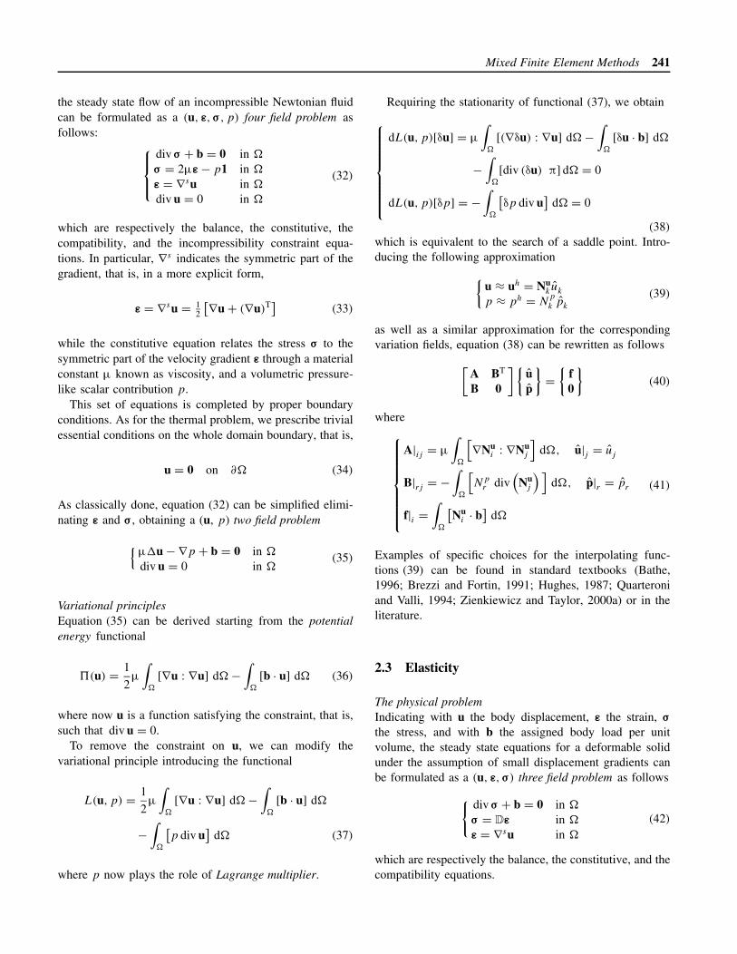
the steady state flow of an incompressible Newtonian fluidcan be formulated as a (u, ε,σ, p) four field problem asfollows:
div σ + b = 0 in �
σ = 2µε − p1 in �
ε = ∇su in �
div u = 0 in �
(32)
which are respectively the balance, the constitutive, thecompatibility, and the incompressibility constraint equa-tions. In particular, ∇s indicates the symmetric part of thegradient, that is, in a more explicit form,
ε = ∇su = 12
[∇u + (∇u)T] (33)
while the constitutive equation relates the stress σ to thesymmetric part of the velocity gradient ε through a materialconstant µ known as viscosity, and a volumetric pressure-like scalar contribution p.
This set of equations is completed by proper boundaryconditions. As for the thermal problem, we prescribe trivialessential conditions on the whole domain boundary, that is,
u = 0 on ∂� (34)
As classically done, equation (32) can be simplified elimi-nating ε and σ, obtaining a (u, p) two field problem
{µ�u − ∇p + b = 0 in �
div u = 0 in �(35)
Variational principlesEquation (35) can be derived starting from the potentialenergy functional
�(u) = 1
2µ
∫�
[∇u : ∇u] d� −∫
�
[b · u] d� (36)
where now u is a function satisfying the constraint, that is,such that div u = 0.
To remove the constraint on u, we can modify thevariational principle introducing the functional
L(u, p) = 1
2µ
∫�
[∇u : ∇u] d� −∫
�
[b · u] d�
−∫
�
[p div u
]d� (37)
where p now plays the role of Lagrange multiplier.
Requiring the stationarity of functional (37), we obtain
dL(u, p)[δu] = µ
∫�
[(∇δu) : ∇u] d� −∫
�
[δu · b] d�
−∫
�
[div (δu) π] d� = 0
dL(u, p)[δp] = −∫
�
[δp div u
]d� = 0
(38)
which is equivalent to the search of a saddle point. Intro-ducing the following approximation{
u ≈ uh = Nuk uk
p ≈ ph = Np
k pk
(39)
as well as a similar approximation for the correspondingvariation fields, equation (38) can be rewritten as follows[
A BT
B 0
]{up
}={
f0
}(40)
where
A|ij = µ
∫�
[∇Nu
i : ∇Nuj
]d�, u|j = uj
B|rj = −∫
�
[Np
r div(
Nuj
) ]d�, p|r = pr
f|i =∫
�
[Nu
i · b]
d�
(41)
Examples of specific choices for the interpolating func-tions (39) can be found in standard textbooks (Bathe,1996; Brezzi and Fortin, 1991; Hughes, 1987; Quarteroniand Valli, 1994; Zienkiewicz and Taylor, 2000a) or in theliterature.
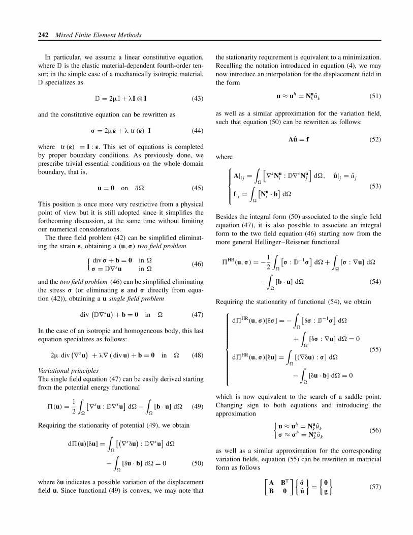
2.3 Elasticity
The physical problemIndicating with u the body displacement, ε the strain, σ
the stress, and with b the assigned body load per unitvolume, the steady state equations for a deformable solidunder the assumption of small displacement gradients canbe formulated as a (u, ε, σ) three field problem as follows{ div σ + b = 0 in �
σ = Dε in �
ε = ∇su in �
(42)
which are respectively the balance, the constitutive, and thecompatibility equations.
242 Mixed Finite Element Methods
In particular, we assume a linear constitutive equation,where D is the elastic material-dependent fourth-order ten-sor; in the simple case of a mechanically isotropic material,D specializes as
D = 2µI + λI ⊗ I (43)
and the constitutive equation can be rewritten as
σ = 2µε + λ tr (ε) I (44)
where tr (ε) = I : ε. This set of equations is completedby proper boundary conditions. As previously done, weprescribe trivial essential conditions on the whole domainboundary, that is,
u = 0 on ∂� (45)
This position is once more very restrictive from a physicalpoint of view but it is still adopted since it simplifies theforthcoming discussion, at the same time without limitingour numerical considerations.
The three field problem (42) can be simplified eliminat-ing the strain ε, obtaining a (u,σ) two field problem{ div σ + b = 0 in �
σ = D∇su in �(46)
and the two field problem (46) can be simplified eliminatingthe stress σ (or eliminating ε and σ directly from equa-tion (42)), obtaining a u single field problem
div(D∇su
)+ b = 0 in � (47)
In the case of an isotropic and homogeneous body, this lastequation specializes as follows:
2µ div(∇su
) + λ∇ ( div u) + b = 0 in � (48)
Variational principlesThe single field equation (47) can be easily derived startingfrom the potential energy functional
�(u) = 1
2
∫�
[∇su : D∇su]
d� −∫
�
[b · u] d� (49)
Requiring the stationarity of potential (49), we obtain
d�(u)[δu] =∫
�
[(∇sδu)
: D∇su]
d�
−∫
�
[δu · b] d� = 0 (50)
where δu indicates a possible variation of the displacementfield u. Since functional (49) is convex, we may note that
the stationarity requirement is equivalent to a minimization.Recalling the notation introduced in equation (4), we maynow introduce an interpolation for the displacement field inthe form
u ≈ uh = Nuk uk (51)
as well as a similar approximation for the variation field,such that equation (50) can be rewritten as follows:
Au = f (52)
whereA|ij =
∫�
[∇sNu
i : D∇sNuj
]d�, u|j = uj
f|i =∫
�
[Nu
i · b]
d�
(53)
Besides the integral form (50) associated to the single fieldequation (47), it is also possible to associate an integralform to the two field equation (46) starting now from themore general Hellinger–Reissner functional
�HR(u,σ) = −1
2
∫�
[σ : D
−1σ]
d� +∫
�
[σ : ∇u] d�
−∫
�
[b · u] d� (54)
Requiring the stationarity of functional (54), we obtain
d�HR(u, σ)[δσ] = −∫
�
[δσ : D
−1σ]
d�
+∫
�
[δσ : ∇u] d� = 0
d�HR(u, σ)[δu] =∫
�
[(∇δu) : σ] d�
−∫
�
[δu · b] d� = 0
(55)
which is now equivalent to the search of a saddle point.Changing sign to both equations and introducing theapproximation {
u ≈ uh = Nuk uk
σ ≈ σh = Nσk σk
(56)
as well as a similar approximation for the correspondingvariation fields, equation (55) can be rewritten in matricialform as follows [
A BT
B 0
]{σ
u
}={
0g
}(57)
Mixed Finite Element Methods 243
where
A|ij =∫
�
[Nσi : D
−1Nσj ] d�, σ|j = σj
B|rj = −∫
�
[∇Nur : Nσ
j ] d�, u|r = ur
g|r = −∫
�
[Nur · b] d�
(58)
Starting from equation (54) the following modified Hellin-ger–Reissner functional can be also generated
�HR,m(u, σ) = −1
2
∫�
[σ : D
−1σ]
d� −∫
�
[u · div σ] d�
−∫
�
[b · u] d� (59)
and, requiring its stationarity, we obtain
d�HR,m(u, σ)[δσ] = −∫
�
[δσ : D
−1σ]
d�
−∫
�
[div (δσ) · u] d� = 0
d�HR,m(u, σ)[δu] = −∫
�
[δu · div σ] d�
−∫
�
[δu · b] d� = 0
(60)
which is again equivalent to the search of a saddle point.Changing sign to both equations and introducing again fieldapproximation (56), equation (60) can rewritten in matricialform as equation (57), with the difference that now
B|rj =∫
�
[Nu
r · div(
Nσj
) ]d� (61)
Similarly, we may also associate an integral form to threefield equation (42) starting from the even more generalHu–Washizu functional
�HW(u, ε,σ) = 1
2
∫�
[ε : Dε] d� −∫
�
[σ :
(ε − ∇su
)]d�
−∫
�
[b · u] d� (62)
Requiring the stationarity of functional (62), we obtain
d�HW(u, ε,σ)[δε] =∫
�
[δε : Dε] d�
−∫
�
[δε : σ] d� = 0
d�HW(u, ε,σ)[δσ] = −∫
�
[δσ :
(ε − ∇su
)]d� = 0
d�HW(u, ε,σ)[δu] =∫
�
[(∇sδu)
: σ]
d�
−∫
�
[δu : b] d� = 0
(63)
which is again equivalent to the search of a saddle point.Introducing the following approximation
u ≈ uh = Nuk uk
ε ≈ εh = Nεk εk
σ ≈ σh = Nσk σk
(64)
as well as a similar approximation for the variation fields,equation (63) can be rewritten as followsA BT 0
B 0 CT
0 C 0
ε
σ
u
=
00h
(65)
where
A|ij =∫
�
[Nε
i : DNεj
]d�, ε|j = εj
B|rj = −∫
�
[Nσ
r : Nεj
]d�, σ|r = σr
C|sr =∫
�
[∇sNus : Nσ
r
]d�, u|s = us
h|s =∫
�
[Nu
s · b]
d�
(66)
For later consideration, we note that equation (65) can berewritten as [
A BT
B 0
]{xy
}={
0h
}(67)
where we made the following simple identifications
A =[
A BT
B 0
], B = {0, C}
x ={
ε
σ
}, y = u (68)
Examples of specific choices for the interpolating func-tions (51), (56), or (64) respectively within the single field,
244 Mixed Finite Element Methods
the two field, and the three field formulations can be foundin standard textbooks (Bathe, 1996; Brezzi and Fortin,1991; Hughes, 1987; Zienkiewicz and Taylor, 2000a) orin the literature.
Toward incompressible elasticityIt is interesting to observe that the strain ε, the stress σ andthe symmetric gradient of the displacement ∇su can beeasily decomposed respectively in a deviatoric (traceless)part and a volumetric (trace-related) part. In particular,recalling that we indicate with d the Euclidean spacedimension, we may set
ε = e + θ
dI with θ = tr (ε)
σ = s + pI with p = tr (σ)
d
∇su = ∇su + div ud
I with div (u) = tr (∇su)
(69)
where θ, p, and div (u) are the volumetric (trace-related)quantities, while e, s, and ∇su are the deviatoric (ortraceless) quantities, that is,
tr (e) = tr (s) = tr(∇su
) = 0 (70)
Adopting these deviatoric-volumetric decompositions andlimiting the discussion for simplicity of notation to thecase of an isotropic material, the three field Hu–Washizufunctional (62) can be rewritten as
�HW,m(u, e, θ, s, p) = 1
2
∫�
[2µe : e + kθ2] d�
−∫
�
[s : (e − ∇su)] d� −∫
�
[p(θ − div u)] d�
−∫
�
[b · u] d� (71)
where we introduce the bulk modulus k = λ + 2µ/d . Ifwe now require a strong (pointwise) satisfaction of thedeviatoric compatibility condition e = ∇su (obtained fromthe stationarity of functional (71) with respect to s) aswell as a strong (pointwise) satisfaction of the volumetricconstitutive equation p = kθ (obtained from the stationarityof functional(71) with respect to θ), we end up with thefollowing simpler modified Hellinger–Reissner functional
�HR,m(u, p) = 1
2
∫�
[2µ∇su : ∇su] d� − 1
2
∫�
[1
kp2] d�
+∫
�
[p div u] d� −∫
�
[b · u] d� (72)
It is interesting to observe that taking the variation of func-tional (72) with respect to p, we obtain the correct relation
between the pressure p and the volumetric component ofthe displacement gradient, that is,
p = k div u =(λ + 2
dµ
)div u (73)
For the case of incompressibility (λ → ∞ and k → ∞),functional (72) reduces to the following form
�HR,m(u, p) = 1
2
∫�
[2µ∇su : ∇su] d� +∫
�
[p div u] d�
−∫
�
[b · u] d� (74)
which resembles the potential energy functional (49) forthe case of an isotropic material with the addition ofthe incompressibility constraint div u = 0 and with thedifference that the quadratic term now involves only thedeviatoric part of the symmetric displacement gradient andnot the whole symmetric displacement gradient.
Requiring the stationarity of functional (74), we obtaind�HR,m(u, p)[δu] =
∫�
[2µ∇sδu : ∇su] d�
+∫
�
[ div (δu) p] d� −∫
�
[δu · b] d� = 0
d�HR,m(u, p)[δp] =∫
�
[δp div u] d� = 0
(75)
Introducing the following approximation{u ≈ uh = Nu
k uk
p ≈ ph = Np
k pk
(76)
as well as a similar approximation for the correspondingvariation fields, equation (75) can be rewritten as follows[
A BT
B 0
]{up
}={
f0
}(77)
where
A|ij = 2µ
∫�
[∇Nu
i : ∇Nuj
]d�, u|j = uj
B|rj =∫
�
[Np
r div(
Nuj
) ]d�, p|r = pr
f|i =∫
�
[Nu
i · b]
d�
(78)
It is interesting to observe that this approach may result inan unstable discrete formulation since the volumetric com-ponents of the symmetric part of the displacement gradientmay not be controlled. Examples of specific choices for the
Mixed Finite Element Methods 245
interpolating functions (76) can be found in standard text-books (Hughes, 1987; Zienkiewicz and Taylor, 2000a) orin the literature.
A different stable formulation can be easily obtained as inthe case of Stokes problem. In particular, we may start fromthe potential energy functional (49), which for an isotropicmaterial specializes as
�(u) = 1
2
∫�
[2µ(∇su : ∇su
)+ λ ( div u)2] d�
−∫
�
[b · u] d� (79)
Introducing now the pressure-like field π = λ div u, we canrewrite functional (79) as
�m(u,π) = 1
2
∫�
[2µ(∇su : ∇su
)− 1
λπ2]
d�
+∫
�
[π div u] d� −∫
�
[b · u] d� (80)
We may note that π is a pressure-like quantity, different,however, from the physical pressure p, previously intro-duced. In fact, π is the Lagrangian multiplier associatedto the incompressibility constraint and it can related to thephysical pressure p recalling relation (73)
p = k div u = π + 2
dµ div u (81)
For the incompressible case (λ → ∞), functional (80) red-uces to the following form:
�m(u, π) = 1
2
∫�
[2µ∇su : ∇su
]d�
+∫
�
[π div u] d� −∫
�
[b · u] d� (82)
Taking the variation of (82) and introducing the followingapproximation {
u ≈ uh = Nuk uk
π ≈ πh = Nπk πk
(83)
as well as a similar approximation for the correspondingvariation fields, we obtain a discrete problem of the fol-lowing form:
[A BT
B 0
]{uπ
}={
f0
}(84)
where
A|ij = 2µ
∫�
[∇sNu
i : ∇sNuj
]d�, u|j = uj
B|rj =∫
�
[Nπ
r div(
Nuj
) ]d�, π|r = πr
f|i =∫
�
[Nu
i · b]
d�
(85)
It is interesting to observe that, in general, this approachresults in a stable discrete formulation since the volumetriccomponents of the symmetric part of the displacementgradient are now controlled. Examples of specific choicesfor the interpolating functions (83) can be found in standardtextbooks (Bathe, 1996; Brezzi and Fortin, 1991; Hughes,1987; Zienkiewicz and Taylor, 2000a) or in the literature.
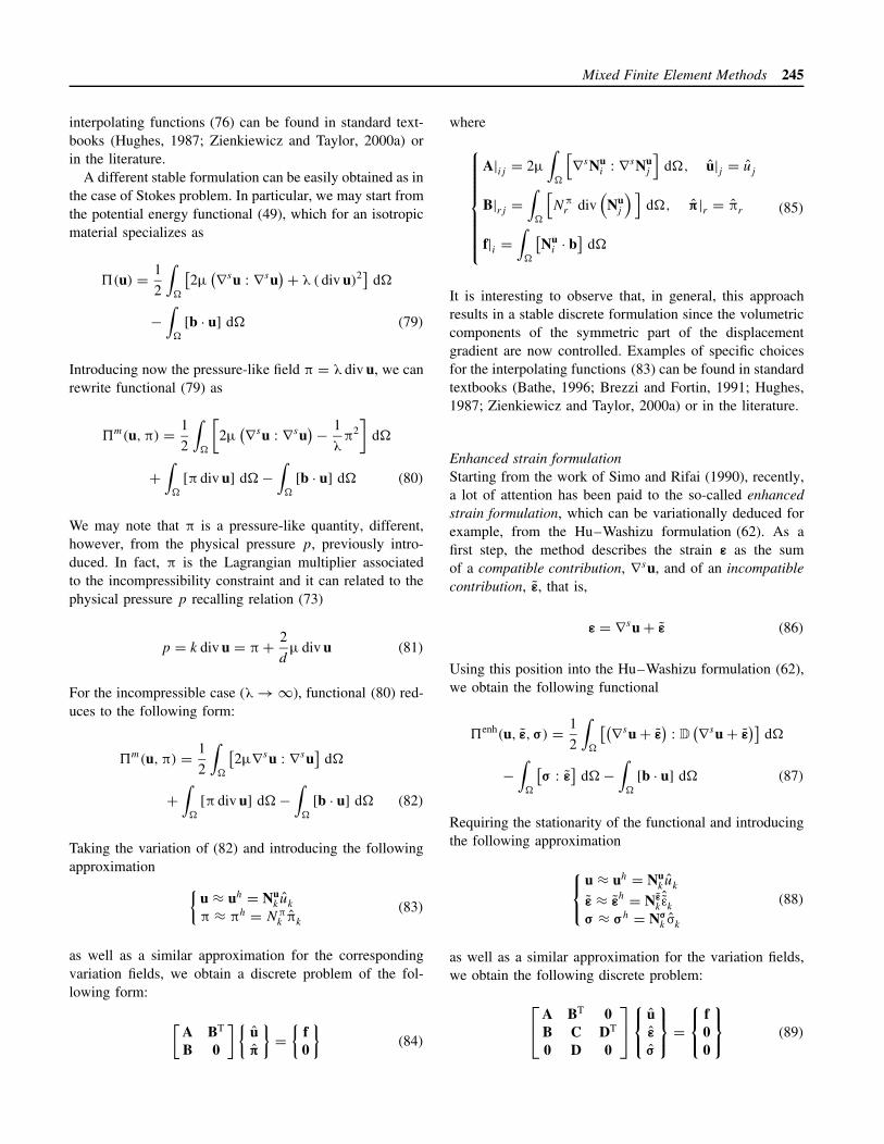
Enhanced strain formulationStarting from the work of Simo and Rifai (1990), recently,a lot of attention has been paid to the so-called enhancedstrain formulation, which can be variationally deduced forexample, from the Hu–Washizu formulation (62). As afirst step, the method describes the strain ε as the sumof a compatible contribution, ∇su, and of an incompatiblecontribution, ε, that is,
ε = ∇su + ε (86)
Using this position into the Hu–Washizu formulation (62),we obtain the following functional
�enh(u, ε, σ) = 1
2
∫�
[(∇su + ε)
: D(∇su + ε
)]d�
−∫
�
[σ : ε
]d� −
∫�
[b · u] d� (87)
Requiring the stationarity of the functional and introducingthe following approximation
u ≈ uh = Nu
k uk
ε ≈ εh = Nεkˆεk
σ ≈ σh = Nσk σk
(88)
as well as a similar approximation for the variation fields,we obtain the following discrete problem:
A BT 0B C DT
0 D 0
uε
σ
=
f00
(89)
246 Mixed Finite Element Methods
where
A|ij =∫
�
[∇sNu
i : D∇sNuj
]d�, u|j = uj
B|rj =∫
�
[Nε
r : D∇sNuj
]d�, ˆε|s = ˆεs
C|rs =∫
�
[Nε
r : DNεs
]d�, σ|r = σr
D|jr = −∫
�
[Nσ
j : Nεr
]d�, f|j =
∫�
[Nu
j · b]
d�
(90)
For later consideration, we note that equation (89) can berewritten as [
A BT
B 0
]{xy
}={
d0
}(91)
where we made the following simple identifications:
A =[
A BT
B C
], B = {0, D}
x ={
uˆε}
, d ={
f0
}, y = σ (92)
Examples of specific choices for the interpolating functionscan be found in standard textbooks (Zienkiewicz and Tay-lor, 2000a) or in the literature.
However, the most widely adopted enhanced strain for-mulation also requires the incompatible part of the strain tobe orthogonal to the stress σ
∫�
[σ : ε
]d� = 0 (93)
If we use conditions (86) and (93) into the Hu–Washizuformulation (62), we obtain the following simplified func-tional:
�enh(u, ε) = 1
2
∫�
[(∇su + ε)
: D(∇su + ε
)]d�
−∫
�
[b · u] d� (94)
which closely resembles a standard displacement-basedincompatible approach. Examples of specific choices for theinterpolating functions involved in this simplified enhancedformulation can be found in standard textbooks(Zienkiewicz and Taylor, 2000a) or in the literature.
3 STABILITY OF SADDLE-POINTS INFINITE DIMENSIONS
3.1 Solvability and stability
The examples discussed in Section 2 clearly show that, afterdiscretization, several formulations typically lead to linearalgebraic systems of the general form[
A BT
B 0
]{xy
}={
fg
}(95)
where A and B are respectively an n × n matrix and anm × n matrix, while x and y are respectively an n × 1vector and m × 1 vector, as well as f and g. Discretizationsleading to such a system are often indicated as mixed finiteelement methods and in the following, we present a simple,algebraic version of the abstract theory that rules mostapplications of mixed methods.
Our first need is clearly to express in proper formsolvability conditions for linear systems of type (95) interms of the properties of the matrices A and B. Bysolvability we mean that for every right-hand side f andg system, (95) has a unique solution. It is well known thatthis property holds if and only if the (n + m) × (n + m)
matrix [A BT
B 0
](96)
is nonsingular, that is, if and only if its determinant isdifferent from zero.
In order to have a good numerical method, however,solvability is not enough. An additional property that wealso require is stability. We want to see this propertywith a little more detail. For a solvable finite-dimensionallinear system, we always have continuous dependence ofthe solution upon the data. This means that there existsa constant c such that for every set of vectors x, y, f, gsatisfying (95) we have
‖x‖ + ‖y‖ ≤ c(‖f‖ + ‖g‖) (97)
This property implies solvability. Indeed, if we assumethat (97) holds for every set of vectors x, y, f, g satisfy-ing (95), then, whenever f and g are both zero, x and ymust also be equal to zero. This is another way of sayingthat the homogeneous system has only the trivial solution,which implies that the determinant of the matrix (96) isdifferent from zero, and hence the system is solvable.
However, Formula (97) deserves another very importantcomment. Actually, we did not specify the norms adoptedfor x, y, f, g. We had the right to do so, since in finite
Mixed Finite Element Methods 247
dimension all norms are equivalent. Hence, the change ofone norm with another would only result in a change of thenumerical value of the constant c, but it would not changethe basic fact that such a constant exists. However, indealing with linear systems resulting from the discretizationof a partial differential equation we face a slightly differentsituation. In fact, if we want to analyze the behaviour ofa given method when the meshsize becomes smaller andsmaller, we must ideally consider a sequence of linearsystems whose dimension increases and approaches infinitywhen the meshsize tends to zero. As it is well known (andit can be also easily verified), the constants involved in theequivalence of different norms depend on the dimension ofthe space. For instance, in R
n, the two norms
‖x‖1 :=n∑
i=1
|xi | and ‖x‖2 :=(
n∑i=1
|xi |2)1/2
(98)
are indeed equivalent, in the sense that there exist twopositive constants c1 and c2 such that
c1‖x‖1 ≤ ‖x‖2 ≤ c2‖x‖1 (99)
for all x in Rn. However, it can be rather easily checked
that the best constants one can choose in (99) are
‖x‖2 ≤ ‖x‖1 ≤ √n‖x‖2 (100)
In particular, the first inequality becomes an equality, forinstance, when x1 is equal to 1 and all the other xi’s arezero, while the second inequality becomes an equality, forinstance, when all the xi are equal to 1.
When considering a sequence of problems with increas-ing dimension, we have to take into account that n and m
become unbounded. It is then natural to ask if, for a givenchoice of the norms ‖x‖, ‖y‖, ‖f‖, and ‖g‖, it is possible tofind a constant c independent of the meshsize (say, h), thatis, a constant c that makes (97) hold true for all meshsizes.
However, even if inequality (97) holds with a constantc independent of h, it will not provide a good concept ofstability unless the four norms are properly chosen (seeRemark 18). This is going to be our next task.
3.2 Assumptions on the norms
We start denoting by X, Y, F, G respectively the spaces ofvectors x, y, f, g. Then, we assume what follows.
1. The spaces X and Y are equipped with norms ‖ · ‖X
and ‖ · ‖Y for which the matrices A and B satisfy thecontinuity conditions: there exist two constants Ma and
Mb, independent of the meshsize, such that for all x andz in X and for all y in Y
xTAz ≤ Ma‖x‖X‖z‖X and xTBTy ≤ Mb‖x‖X‖y‖Y
(101)
Moreover, we suppose there exist symmetric positivedefinite matrices Mx and My , respectively of dimen-sions n × n and m × m, such that
‖x‖2X = xTMxx ∀ x ∈ X (102)
and
‖y‖2Y = yTMyy ∀ y ∈ Y (103)
2. The spaces F and G are equipped with norms ‖ · ‖F and‖ · ‖G defined as the dual norms of ‖ · ‖X and ‖ · ‖Y ,that is,
‖f‖F := supx∈X\{0}
xTf‖x‖X
and ‖g‖G := supy∈Y\{0}
yTg‖y‖Y
(104)
It is worth noting that
• assumptions (102) to (103) mean that the norms forX and Y are both induced by an inner product or, inother words, the norms at hand are hilbertian (as ithappens in most of the applications);
• for every x and f in Rn and for every y and g in R
m,we have
xTf ≤ ‖x‖X‖f‖F and yTg ≤ ‖y‖Y‖g‖G
(105)
• combining the continuity condition (101) on || · ||Xand || · ||Y with the dual norm definition (105), forevery x ∈ X and for every y ∈ Y, we have the fol-lowing relations:
‖Ax‖F = supz∈X\{0}
zTAx‖z‖X
≤ Ma‖x‖X (106)
‖Bx‖G = supz∈Y\{0}
zTBx‖z‖X
≤ Mb‖x‖X (107)
‖BTy‖F = supz∈X\{0}
zTBTy‖z‖X
≤ Mb‖y‖Y (108)
• if A is symmetric and positive semidefinite, then forevery x, z ∈ X
|zTAx| ≤ (zTAz)1/2(xTAx)1/2 (109)
248 Mixed Finite Element Methods
so that (106) can be improved to
‖Ax‖F ≤ supz∈X\{0}
zTAx‖z‖X
≤ M1/2a (xTAx)1/2 (110)
We are now ready to introduce a precise definition ofstability.
Stability definition. Given a numerical method, that pro-duces a sequence of matrices A and B when applied to agiven sequence of meshes (with the meshsize h going tozero), we choose norms ‖ · ‖X and ‖ · ‖Y that satisfy thecontinuity condition (101), and dual norms ‖ · ‖F and ‖ · ‖G
according to (104). Then, we say that the method is sta-ble if there exists a constant c, independent of the mesh,such that for all vectors x, y, f, g satisfying the general sys-tem (95), it holds
‖x‖X + ‖y‖Y ≤ c(‖f‖F + ‖g‖G) (111)
Having now a precise definition of stability, we can lookfor suitable assumptions on the matrices A and B that mayprovide the stability result (111). In particular, to guar-antee stability condition (111), we need to introduce twoassumptions involving such matrices. The first assumption,the so-called inf–sup condition, involves only the matrix Band it will be used throughout the whole section. To illus-trate the second assumption we will first focus on a simplerbut less general case that involves a ‘strong’ requirement onthe matrix A. Among the problems presented in Section 2,this requirement is verified in practice only for the Stokesproblem. Then, we shall tackle a more complex and clearlymore general case, corresponding to a ‘weak’ requirementon the matrix A, suited for instance for discretizations ofthe mixed formulations of thermal diffusion problems.
Later on we shall deal with some additional complica-tions that occur for instance, in the (u, π)-formulation ofnearly incompressible elasticity (cf. (80)). Finally, we shallbriefly discuss more complicated problems, omitting theproofs for simplicity.
3.3 A requirement on the B matrix: the inf–supcondition
The basic assumption that we are going to use, throughoutthe whole section, deals with the matrix B. We assume thefollowing:
Inf–sup condition. There exists a positive constant β,independent of the meshsize h, such that:
∀ y ∈ Y ∃x ∈ X \ {0} such that xTBTy ≥ β‖x‖X‖y‖Y
(112)
Condition (112) requires the existence of a positive con-stant β, independent of h, such that for every y ∈ Y we canfind a suitable x ∈ X, different from 0 (and depending ony), such that (112) holds.
Remark 1. To better understand the meaning of (112), itmight be useful to see when it fails. We thus consider thefollowing m × n pseudodiagonal matrix (m < n)
B =
ϑ1 0 · · · 0 · · · · 00 ϑ2 0 · · · · · · · ·· · · · · · · · · · ·· · · · 0 · · · · · ·0 · · 0 ϑm 0 · · · · 0
(113)
with 0 ≤ ϑ1 ≤ ϑ2 ≤ ·· ≤ ϑm ≤ 1. To fix ideas, we supposethat both X ≡ R
n and Y ≡ Rm are equipped with the stan-
dard Euclidean norms, which coincide with the correspond-ing dual norms on F and G (cf. (104)). If ϑ1 = 0, choosingy = (1, 0, . . . , 0)T �= 0, we have BTy = 0. Therefore, forevery x ∈ X, we get xTBTy = 0 and condition (112) cannothold since β must be positive. We then infer that condi-tion (112) requires that
no y �= 0 satisfies BTy = 0
which, by definition, means that BT is injective. However,the injectivity of BT is not sufficient for the fulfillment ofcondition (112). Indeed, for 0 < ϑ1 ≤ ϑ2 ≤ · · · ≤ ϑm ≤ 1,the matrix BT is injective and we have, still choosingy = (1, 0, . . . , 0)T,
BTy = (ϑ1, 0, . . . , 0)T �= 0 (114)
Since for every x ∈ X it holds
xTBTy = ϑ1x1 ≤ ϑ1||x||X = ϑ1||x||X||y||Y (115)
we obtain that the constant β in (112) is forced to satisfy
0 < β ≤ ϑ1 (116)
As a consequence, if ϑ1 > 0 tends to zero with the meshsizeh, the matrix BT is still injective but condition (112) fails,because β, on top of being positive, must be independentof h. Noting that (see (114))
‖BTy‖F
‖y‖Y
= ϑ1 (117)
we then deduce that condition (112) requires that for y �= 0
the vector BTy is not ‘too small’ with respect to y

Mixed Finite Element Methods 249
which is a property stronger than the injectivity of thematrix BT. We will see in Proposition 1 that all theseconsiderations on the particular matrix B in (113) doesextend to the general case.
We now rewrite condition (112) in different equivalentforms, which will also make clear the reason why it iscalled inf–sup condition.
Since, by assumption, x is different from zero, condi-tion (112) can equivalently be written as
∀ y ∈ Y ∃x ∈ X\{0} such thatxTBTy‖x‖X
≥ β‖y‖Y
(118)
This last form (118) highlights that given y ∈ Y, the mostsuitable x ∈ X is the one that makes the left-hand sideof (118) as big as possible. Hence, the best we can do isto take the supremum of the left-hand side, when x variesamong all possible x ∈ X different from 0. Hence, we mayequivalently require that
∀ y ∈ Y supx∈X\{0}
xTBTy‖x‖X
≥ β‖y‖Y (119)
In a sense, we got rid of the task of choosing x. However,condition (119) still depends on y and it clearly holds fory = 0. Therefore, we can concentrate on the y’s that aredifferent from 0; in particular, for y �= 0 condition (119)can be also written as
supx∈X\{0}
xTBTy‖x‖X‖y‖Y
≥ β (120)
The worst possible y is therefore the one that makes the left-hand side of (120) as small as possible. If we want (120) tohold for every y ∈ Y we might as well consider the worstcase, looking directly at the infimum of the left-hand sideof (120) among all possible y’s, requiring that
infy∈Y\{0} sup
x∈X\{0}xTBTy
‖x‖X‖y‖Y
≥ β (121)
The advantage of formulation (121), if any, is that we gotrid of the dependency on y as well. Indeed, condition (121)is now a condition on the matrix B, on the spaces X andY (together with their norms) as well as on the crucialconstant β.
Let us see now the relationship of the inf–sup conditionwith a basic property of the matrix B.
Proposition 1. The inf–sup condition (112) is equivalentto require that
β‖y‖Y ≤ ‖BTy‖F ∀ y ∈ Y (122)
Therefore, in particular, the inf–sup condition implies thatthe matrix BT is injective.
Proof. Assume that the inf–sup condition (112) holds, andlet y be any vector in Y. By the equivalent form (119) andusing definition (104) of the dual norm ‖ · ‖F , we have
β‖y‖Y ≤ supx∈X\{0}
xTBTy‖x‖X
= ‖BTy‖F (123)
and therefore (122) holds true. Moreover, the matrix BT isinjective since (122) shows that y �= 0 implies BTy �= 0.
Assume conversely that (122) holds. Using again thedefinition (104) of the dual norm ‖ · ‖F , we have
β‖y‖Y ≤ ‖BTy‖F = supx∈X\{0}
xTBTy‖x‖X
(124)
which implies the inf–sup condition in the form (119).
Remark 2. Whenever the m × n matrix B satisfies theinf–sup condition, the injectivity of BT implies that n ≥ m.We point out once again (cf. Remark 1) that the injectivityof BT is not sufficient for the fulfillment of the inf–supcondition.
Additional relationships between the inf–sup and otherproperties of the matrix B will be presented later on inSection 3.5.
3.4 A ‘strong’ condition on the A matrix.Ellipticity on the whole space — Stokes
As we shall see in the sequel, the inf–sup condition is anecessary condition for having stability of problems of thegeneral form (95). In order to have sufficient conditions,we now introduce a further assumption on the matrix A.As discussed at the end of Section 3.2, we start consideringa strong condition on the matrix A. More precisely, weassume the following:
Ellipticity condition. There exists a positive constant α,independent of the meshsize h, such that
α‖x‖2X ≤ xTAx ∀ x ∈ X (125)
We first notice that from (101) and (125) it follows that
α ≤ Ma (126)
We have now the following theorem.
Theorem 1. Let x, y, f, g satisfy the general system ofequations (95). Moreover, assume that A is symmetric and
250 Mixed Finite Element Methods
that the continuity conditions (101), the dual norm assump-tions (105), the inf–sup (112) and the ellipticity require-ment (125) are all satisfied. Then, we have
‖x‖X ≤ 1
α‖f‖F + M
1/2a
α1/2β‖g‖G (127)
‖y‖Y ≤ 2M1/2a
α1/2β‖f‖F + Ma
β2‖g‖G (128)
Proof. We shall prove the result by splitting x = xf + xg
and y = yf + yg defined as the solutions of{Axf + BTyf = fBxf = 0 (129)
and {Axg + BTyg = 0Bxg = g (130)
We proceed in several steps.• Step 1 – Estimate of xf and Axf We multiply the firstequation of (129) to the left by xT
f and we notice thatxTf BTyf ≡ yTBxf = 0 (by the second equation). Hence,
xTf Axf = xTf (131)
and, using the ellipticity condition (125), relation (131),and the first of the dual norm estimates (105), we have
α‖xf ‖2X ≤ xT
f Axf = xTf ≤ ‖xf ‖X‖f‖F (132)
giving immediately
‖xf ‖X ≤ 1
α‖f‖F (133)
and
xTf Axf ≤ 1
α‖f‖2
F (134)
Therefore, using (110) we also get
‖Axf ‖F ≤ M1/2a
α1/2‖f‖F (135)
• Step 2 – Estimate of yf We use now the inf–sup con-dition (112) with y = yf . We obtain that there exists x ∈X such that xTBTyf ≥ β‖x‖X‖yf ‖Y . Multiplying the firstequation of (129) by xT and using the first of the dual normestimates (105), we have
β‖x‖X‖yf ‖Y ≤ xTBTyf = xT(f − Axf )
≤ ‖x‖X‖f − Axf ‖F (136)
We now use the fact that in the inf–sup condition (112)we had x �= 0, so that in the above equation (136) wecan simplify by its norm. Then, using (135) and (126), weobtain
‖yf ‖Y ≤ 1
β‖f − Axf ‖F ≤
(1
β+ M
1/2a
α1/2β
)‖f‖F
≤ 2M1/2a
α1/2β‖f‖F (137)
• Step 3 – Estimate of xTgAxg by ‖yg‖Y We multiply the
first equation of (130) by xTg . Using the second equation
of (130) and the second of the dual norm estimates (105),we have
xTgAxg = −xT
gBTyg ≡ yTgBxg = yT
gg ≤ ‖yg‖Y ‖g‖G (138)
• Step 4 – Estimate of ‖yg‖Y by (xTgAxg)
1/2 We proceedas in Step 2. Using the inf–sup condition (112) with y = yg
we get a new vector, that we call again x, such thatxTBTyg ≥ β‖x‖X‖yg‖Y . This relation, the first equationof (130), and the continuity property (109) yield
β‖x‖X‖yg‖Y ≤ xTBTyg = −xTAxg
≤ M1/2a ‖x‖X(xT
gAxg)1/2 (139)
giving
‖yg‖Y ≤ M1/2a
β(xT
gAxg)1/2 (140)
• Step 5 – Estimate of ‖xg‖X and ‖yg‖Y We first com-bine (138) and (140) to obtain
‖yg‖Y ≤ Ma
β2‖g‖G (141)
Moreover, using the ellipticity assumption (125) in (138)and inserting (141), we have
α‖xg‖2X ≤ xT
gAxg ≤ ‖yg‖Y ‖g‖G ≤ Ma
β2‖g‖2
G (142)
which can be rewritten as
‖xg‖X ≤ M1/2a
α1/2β‖g‖G (143)
The final estimate follows then by simply collecting theseparate estimates (133), (137), (143), and (141).
A straightforward consequence of Theorem 1 and Re-mark 4 is the following stability result (cf. (111)):

Mixed Finite Element Methods 251
Corollary 1. Assume that a numerical method produces asequence of matrices A and B for which both the inf–supcondition (112) and the ellipticity condition (125) are satis-fied. Then the method is stable.
Remark 3. In certain applications, it might happen thatthe constants α and β either depend on h (and tend to zero ash tends to zero) or have a fixed value that is however verysmall. It is therefore important to keep track of the possibledegeneracy of the constants in our estimates when α and/orβ are very small. In particular, it is relevant to know whetherour stability constants degenerate, say, as 1/β, or 1/β2, orother powers of 1/β (and, similarly, of 1/α). In this respect,we point out that the behavior indicated in (127) and (128)is optimal. This means that we cannot hope to find a betterproof giving a better behavior of the constants in terms ofpowers of 1/α and 1/β. Indeed, consider the system
2√
a b√a a 0
b 0 0
x1x2y
=
f1f2g
0 < a, b � 1
(144)
whose solution is
x1 = g
b, x2 = f2
a− g
a1/2b, y = f1
b− f2
a1/2b− g
b2
(145)
Since the constants α and β are given by
α = 2 + a − √a2 + 4
2= 4a
2(
2 + a + √a2 + 4
) ≈ a
and
β = b
we see from (145) that there are cases in which theactual stability constants behave exactly as predicted bythe theory.
Remark 4. We point out that the symmetry conditionon the matrix A is not necessary. Indeed, with a slightlydifferent (and even simpler) proof one can prove stabilitywithout the symmetry assumption. The dependence of thestability constant upon α and β is however worse, as it canbe seen in the following example. Considering the system
1 −1 b
1 a 0b 0 0
x1x2y
=
f1f2g
0 < a, b � 1
(146)
one easily obtains
x1 = g
b, x2 = f2
a− g
ab, y = f1
b+ f2
ab− (1 + a)g
ab2
(147)
Since α = a and β = b, from (147) we deduce that thebounds of Theorem 1 cannot hold when A is not symmetric.
As announced in the title of the section the situation inwhich A is elliptic in the whole space is typical (amongothers) of the Stokes problem, as presented in (22) to (24).Indeed, denoting the interpolating functions for u and p byNu
i and Npr respectively (cf. (39)), if we set
‖u‖2X := µ
∫�
∣∣∇(Nui ui )
∣∣2 d� (148)
and
‖p‖2Y :=
∫�
∣∣Npr pr
∣∣2 d� (149)
we can easily see that conditions (101) are verified withMa = 1 and Mb = √
(d/µ) respectively. Clearly the ellip-ticity property (125) is also verified with α = 1, no matterwhat is the choice of the mesh and of the interpolatingfunctions. On the other hand, the inf–sup Property (112) ismuch less obvious, as we are going to see in Section 4, andfinite element choices have to be specially tailored in orderto satisfy it.
3.5 The inf–sup condition and the liftingoperator
In this section, we shall see that the inf–sup conditionis related to another important property of the matrix B.Before proceeding, we recall that an m × n matrix B issurjective if for every g ∈ R
m, there exists xg ∈ Rn such
that Bxg = g.We have the following Proposition.
Proposition 2. The inf–sup condition (112) is equivalentto require the existence of a lifting operator L: g → xg =Lg such that, for every g ∈ R
m, it holds{Bxg = gβ‖xg‖X ≡ β‖Lg‖X ≤ ‖g‖G ≡ ‖Bxg‖G
(150)
Therefore, in particular, the inf–sup condition implies thatthe matrix B is surjective.
Proof. We begin by recalling that there exists a symmetric(n × n) positive definite matrix Mx such that (cf. (102))
xTMxx = ‖x‖2X (151)

252 Mixed Finite Element Methods
It is clear that the choice A ≡ Mx easily satisfies the firstof the continuity conditions (101) with Ma = 1, as well asthe ellipticity condition (125) with α = 1. Given g, if theinf–sup condition holds, we can, therefore, use Theorem1 and find a unique solution (xg, yg) of the followingauxiliary problem:{
Mx xg + BTyg = 0,
Bxg = g (152)
We can now use estimate (143) from Step 5 of the proofof Theorem 1, recalling that in our case, α = Ma = 1 sincewe are using the matrix Mx instead of A. We obtain
β‖xg‖X ≤ ‖g‖G (153)
It is then clear that setting Lg := xg (the first part ofthe solution of the auxiliary problem (152)) we have thatestimate (150) in our statement holds true.
Assume conversely that we have the existence of acontinuous lifting L satisfying (150). First we recall thatthere exists a symmetric (m × m) positive definite matrixMy such that (cf. (103))
yTMyy = ‖y‖2Y (154)
Then, for a given y ∈ Y, we set first g := Myy (so thatyTg = ‖y‖2
Y ) and then we define xg := Lg (so that Bxg =g). Hence,
xTgBTy ≡ yTBxg = yTg = yTMyy = ‖y‖2
Y (155)
On the other hand, it is easy to see that using (150) wehave
β‖xg‖X ≤ ‖g‖G ≤ ‖y‖Y (156)
where the last inequality is based on the choice g = Myyand the use of (108) with My in the place of BT. Hence,for every y ∈ Y, different from zero, we constructed x =xg ∈ X, different from zero, which, joining (155) and (156),satisfies
xTgBTy = ‖y‖2
Y ≥ β‖xg‖X‖y‖Y (157)
that is, the inf–sup condition in its original form (112).
3.6 A ‘weak’ condition on the A matrix.Ellipticity on the kernel — thermal diffusion
We now consider that, together with the inf–sup conditionon B, the condition on A is weaker than the full Elliptic-ity (125). In particular, we require the ellipticity of A to
hold only in a subspace X0 of the whole space X, with X0defined as follows:
X0 := Ker(B) ≡ {x ∈ X such that Bx = 0} (158)
More precisely, we require the following:
Elker condition. There exists a positive constant α0, inde-pendent of the meshsize h, such that
α0‖x‖2X ≤ xTAx ∀ x ∈ X0 (159)
The above condition is often called elker since itrequires the ellipticity on the kernel. Moreover, from (101)and (159), we get
α0 ≤ Ma (160)
The following theorem generalizes Theorem 1. For the sakeof completeness, we present here the proof in the case of amatrix A that is not necessarily symmetric.
Theorem 2. Let x ∈ X and y ∈ Y satisfy system (1) andassume that the continuity conditions (101), the dual normassumptions (105), the inf–sup (112), and the elker condi-tion (159) are satisfied. Then, we have
‖x‖X ≤ 1
α0‖f‖F + 2Ma
α0β‖g‖G (161)
‖y‖Y ≤ 2Ma
α0β‖f‖F + 2M2
a
α0β2‖g‖G (162)
Proof. We first set xg := Lg where L is the lifting operatordefined by Proposition 2. We also point out the followingestimates on xg: from the continuity of the lifting L (150),we have
β‖xg‖X ≤ ‖g‖G (163)
and using (106) and (163), we obtain
‖Axg‖F ≤ Ma‖xg‖X ≤ Ma
β‖g‖G (164)
Then, we set
x0 := x − xg = x − Lg (165)
and we notice that x0 ∈ X0. Moreover, (x0, y) solves thelinear system {
Ax0 + BTy = f − Axg,
Bx0 = 0(166)
We can now proceed as in Steps 1 and 2 of the proof ofTheorem 1 (as far as we do not use (110), since we gave
Mixed Finite Element Methods 253
up the symmetry assumption). We note that our weakerassumption elker (159) is sufficient for allowing the firststep in (132). Proceeding as in the first part of Step 1, andusing (164) at the end, we get
‖x0‖X ≤ 1
α0‖f − Axg‖F ≤ 1
α0
(‖f‖F + Ma
β‖g‖G
)(167)
This allows to reconstruct the estimate on x:
‖x‖X = ‖x0 + xg‖X ≤ 1
α0‖f‖F +
(Ma
α0β+ 1
β
)‖g‖G
≤ 1
α0‖f‖F + 2Ma
α0β‖g‖G (168)
where we have used (160) in the last inequality. Combin-ing (106) and (168), we also have
‖Ax‖F ≤ Ma‖x‖X ≤ Ma
α0
‖f‖F + 2M2a
α0β‖g‖G (169)
which is weaker than (135) since we could not use thesymmetry assumption. Then, we proceed as in Step 2 toobtain, as in (137)
β‖y‖Y ≤ ‖f − Ax‖F (170)
and using the above estimate (169) on Ax in (170), weobtain
‖y‖Y ≤(
1
β+ Ma
α0β
)‖f‖F + 2M2
a
α0β2‖g‖G
≤ 2Ma
α0β‖f‖F + 2M2
a
α0β2‖g‖G (171)
and the proof is concluded.
A straightforward consequence of Theorem 2 is the fol-lowing stability result (cf. (111)):
Corollary 2. Assume that a numerical method produces asequence of matrices A and B for which both the inf–supcondition (112) and the elker condition (159) are satisfied.Then the method is stable.
Remark 5. In the spirit of Remark 3, we notice that thedependence of the stability constants from α0 and β isoptimal, as shown by the previous example (146), for whichα0 = a and β = b. It is interesting to notice that just addingthe assumption that A is symmetric will not improve thebounds. Indeed, considering the system 1 1 b
1 a 0b 0 0
x1x2y
=
f1f2g
0 < a, b � 1 (172)
one easily obtains
x1 = g
b, x2 = f2
a− g
ab, y = f1
b− f2
ab+ (1 − a)g
ab2
(173)
Since α0 = a and β = b, system (172) shows the samebehavior as the bounds of Theorem 2 (and not better), eventhough A is symmetric. In order to get back the betterbounds found in Theorem 1, we have to assume that A,on top of satisfying the ellipticity in the kernel (159), issymmetric and positive semidefinite in the whole R
n (aproperty that the matrix A in (172) does not have for 0 ≤a < 1). This is because, in order to improve the bounds, onehas to use (110) that, indeed, requires A to be symmetricand positive semidefinite.
As announced in the title of the section, the situation inwhich A is elliptic only in the kernel of B is typical (amongothers) of the mixed formulation of thermal problems, aspresented in (22) to (24). As in (19), we denote the inter-polating functions for θ and q by N θ
r and Nqi , respectively,
and we set
‖q‖2X :=
∫�
[(Nq
i qi
) · D−1(
Nqj qj
)]d�
+ �2
k∗
∫�
|div (Nqi qi )|2 d� (174)
‖θ‖2Y :=
∫�
|N θr θr |2 d� (175)
where � represents some characteristic length of the domain� (for instance its diameter) and k∗ represent some charac-teristic value of the thermal conductivity (for instance, itsaverage).
We can easily see that the continuity conditions (101) areverified with Ma = 1 and Mb = �−1√k∗ respectively. Onthe other hand, the full ellipticity property (125) is verifiedonly with a constant α that behaves, in most cases, likeα � h2, where h is a measure of the mesh size. Indeed,the norm of q contains the derivatives of the interpolatingfunctions, while the term qTAq does not, as it can beseen in (21). On the other hand, we are obliged to add thedivergence term in the definition (174) of the norm of q:otherwise, we cannot have a uniform bound for Mb whenthe meshsize goes to zero, precisely for the same reason
as before. Indeed, the term θTBq contains the derivatives
of the interpolating functions Nqi (see (21)), and the first
part of ‖q‖X does not. One can object that the constantMb does not show up in the stability estimates. It does,however, come into play in the error estimates, as we aregoing to see in Section 5.
It follows from this analysis that, keeping the normsas in (174) and (175), the elker property (159) holds, in
254 Mixed Finite Element Methods
practical cases, only if the kernel of B is made of free-divergence vectors. In that case, we would actually haveα0 = 1, no matter what is the choice of the mesh and ofthe interpolating functions.
On the other hand, the inf–sup property (112) is stilldifficult and it depends heavily on the choices of theinterpolating functions. As we are going to see in the nextsection, the need to satisfy both the elker and the inf–supcondition poses serious limitations on the choice of theapproximations. Apart from some special one-dimensionalcases, there is no hope that these two properties can holdat the same time unless the finite element spaces havebeen designed for that. However, this work has beenalready done and there are several families of finite elementspaces that can be profitably used for these problems. Wealso note that the elker condition (or, more precisely, therequirement that the kernel of B is made only of free-divergence vectors) poses some difficulties in the choice ofthe element, but in most applications it constitutes a verydesirable conservation property for the discrete solutions.
3.7 Perturbation of the problem — nearlyincompressible elasticity
We now consider a possible variant of our general form(95). Namely, we assume that we have, together with thematrices A and B, a third matrix C, that we assume to bean (m × m) matrix, and we consider the general form[
A BT
B −C
]{xy
}={
fg
}(176)
For simplicity, we assume that the matrix C is given byC = εMy , where the matrix My is attached to the norm‖ · ‖Y as in (103). Clearly, the results will apply, almostunchanged, to a symmetric positive definite matrix havingmaximum and minimum eigenvalue of order ε. We havethe following result.
Theorem 3. Let x ∈ X and y ∈ Y satisfy the system{Ax + BTy = fBx − εMyy = g
(177)
Assume that A is symmetric and positive semidefinite, andthat the continuity condition (101), the dual norm assump-tions (105), the inf–sup (112) and the elker condition (159)are satisfied. Then, we have
‖x‖X ≤ β2 + 4εMa
α0β2
‖f‖F + 2M1/2a
α1/20 β
‖g‖G (178)
and
‖y‖Y ≤ 2M1/2a
α1/20 β
‖f‖F + 4Ma
Maε + β2‖g‖G (179)
Proof. The proof can be performed with arguments similarto the ones used in the previous stability proofs, but usingmore technicalities. For simplicity, we are going to giveonly a sketch, treating separately the two cases f = 0 andg = 0.
• The case f = 0. We set x = L(g + εMyy) and x0 = x −x. Proceeding exactly as in the proof of Theorem 1 (Step4 ), we obtain inequality (140):
‖y‖Y ≤ M1/2a
β(xTAx)1/2 (180)
Then, we multiply the first equation of (176) times xT andsubstitute the value of y obtained from the second equation.We have
xTAx + 1
ε
[(My)−1(Bx − g)
]TBx = 0 (181)
Using the fact that xTAx > 0, we easily deduce that
‖Bx‖G ≤ ‖g‖G (182)
This implies
‖x‖X ≤ 1
β‖Bx‖G ≤ 1
β‖g‖G (183)
We now multiply the first equation times xT0 , and we have
xT0 Ax = 0. We can then use (109) to get
xT0 Ax0 = −xT
0 Ax ≤ (xT0 Ax0)
1/2(xTAx)1/2 (184)
Simplifying by (xT0 Ax0)
1/2 and using (183), we obtain
xT0 Ax0 ≤ xTAx ≤ Ma ‖x‖2
X ≤ Ma
β2‖g‖2
G (185)
Using x = x0 + x, and then again (109) and (183), weobtain
xTAx ≤ 4Ma
β2‖g‖2
G (186)
that inserted in (180) gives an estimate for y
‖y‖Y ≤ 2Ma
β2‖g‖G (187)
Mixed Finite Element Methods 255
On the other hand, using the elker condition (159), esti-mates (183), (185), and (160) we have
‖x‖X ≤ ‖x0‖X + ‖x‖X ≤(
M1/2a
α1/20 β
+ 1
β
)‖g‖G
= M1/2a + α
1/20
α1/20 β
‖g‖G ≤ 2M1/2a
α1/20 β
‖g‖G (188)
However, we note that using the second equation we mighthave another possible estimate for y:
‖y‖Y ≤ 1
ε‖Bx − g‖G ≤ 2
ε‖g‖G (189)
We can combine (187) and (189) into
‖y‖Y ≤ min{
2
ε,
2Ma
β2
}‖g‖G ≤ 4Ma
Maε + β2‖g‖G (190)
• The case g = 0. We set this time x = L(εMyy) and againx0 := x − x. From (150), we have as usual
‖x‖X ≤ 1
β‖Bx‖G ≡ 1
β‖Bx‖G (191)
Multiplying the first equation by xT0 , we have xT
0 Ax = x0fthat gives, using (159) and (109)
xT0 Ax0 ≤ 1
α1/20
‖f‖F (xT0 Ax0)
1/2 + (xT0 Ax0)
1/2(xTAx)1/2
(192)
and finally,
(xT0 Ax0)
1/2 ≤ 1
α1/20
‖f‖F + (xTAx)1/2 (193)
In particular, using once more, (109), (193), and (191), weobtain
|xT0 Ax| ≤ 1
α1/20
‖f‖F (xTAx)1/2 + xTAx
≤ M1/2a
α1/20 β
‖f‖F ‖Bx‖G + xTAx (194)
Take now the product of the first equation times xT andusing y = ε−1(My)−1Bx from the second equation, we havexTBTy = ε−1xTBT(My)−1Bx = ε−1‖Bx‖2
G. Hence,
xTAx + 1
ε‖Bx‖2
G = xTf ≤ 1
β‖f‖F‖Bx‖G (195)
Using xTAx = xTAx + xTAx0 and the estimate (194)in (195), we deduce
1
ε‖Bx‖2
G ≤ 1
β‖f‖F‖Bx‖G + M
1/2a
α1/20 β
‖f‖F‖Bx‖G (196)
that finally gives
‖Bx‖G ≤ ε
(1
β+ M
1/2a
α1/20 β
)‖f‖F ≤ 2εM
1/2a
α1/20 β
‖f‖F (197)
which is a crucial step in our proof. Indeed, from (197) andthe second equation, we obtain our estimate for y
‖y‖Y ≤ 1
ε‖Bx‖G ≤ 2M
1/2a
α1/20 β
‖f‖F (198)
From (191) and (197), we have
‖x‖X ≤ 1
β‖Bx‖G ≤ 2εM
1/2a
α1/20 β2
‖f‖F (199)
Finally, from (159), (193), and (199), we obtain
‖x0‖X ≤ 1
α1/20
(xT0 Ax0)
1/2 ≤(
1
α0
+ 2εMa
α0β2
)‖f‖F
= β2 + 2εMa
α0β2
‖f‖F (200)
which together with (199) gives us the estimate for x
‖x‖X ≤(
2εM1/2a
α1/20 β2
+ 2εMa + β2
α0β2
)‖f‖F ≤ 4εMa + β2
α0β2
‖f‖F
(201)
Collecting (190), (188), (198), and (201), we have theresult.
Remark 6. We notice that the dependence of the stabilityconstants upon α0 and β in Theorem 3 are optimal, as shownby the system
2a√
a −√a 0 0√
a 2 1 b 0−√
a 1 2 0 b
0 b 0 −ε 00 0 b 0 −ε
x1x2x3y1y2
=
2f
000
2g
0 < a, b, ε � 1 (202)
Indeed, we have α0 = 2a, β = b, and the solution is givenby
x1 = f (b2 + ε)
ab2+ g
a1/2b, x2 = − f ε
a1/2b2− 3gε
b(3ε + b2),
256 Mixed Finite Element Methods
x3 = f ε
a1/2b2+ g(3ε + 2b2)
b(3ε + b2),
y1 = − f
a1/2b− 3g
3ε + b2, y2 = f
a1/2b− 3g
3ε + b2
Remark 7. It is also worth noticing that assuming fullellipticity of the matrix A as in (125) (instead of ellipticityonly in the kernel as we did here) would improve theestimates for x. In particular, we could obtain estimates thatdo not degenerate when β goes to zero, as far as ε remainsstrictly positive. For the case f = 0, this is immediate fromthe estimate of y (190): from the first equation, we haveeasily
‖x‖ ≤ 1
αMb‖y‖Y ≤ 4MaMb
α(Maε + β2)‖g‖G (203)
In the case g = 0, we can combine the two equations to get
xTAx + ε‖y‖2Y = xTf (204)
that gives (always using (125))
‖x‖X ≤ 1
α‖f‖F (205)
that then gives
‖y‖Y ≤ 1
ε‖Bx‖G ≤ Mb
εα‖f‖F (206)
This could be combined with (198) into
‖y‖Y ≤ min
{Mb
εα,
2M1/2a
α1/2β
}‖f‖F
≤ 4M1/2a Mb
2M1/2a αε + α1/2βMb
‖f‖F (207)
Collecting the two cases we have
‖x‖X ≤ 1
α‖f‖F + 4MaMb
α1/2(Maε + β2)‖g‖G (208)
and
‖y‖Y ≤ 4M1/2a Mb
2M1/2a αε + α1/2βMb
‖f‖F + 4Ma
Maε + β2‖g‖G
(209)
which do not degenerate for β going to zero.
As announced in the title of the section, systems ofthe type (176) occur, for instance, in the so-called (u,π)
formulation of nearly incompressible elasticity. Sometimesthey are also obtained by penalizing systems of the originaltype (95) in order to obtain a partial cure in cases in which
β is zero or tending to zero with the meshsize (as it couldhappen, for instance, for a discretization of Stokes problemthat does not satisfy the inf–sup condition), in the spiritof Remark 7. Indeed, the (u, π) formulation of nearlyincompressible elasticity, in the case of an isotropic andhomogeneous body, could be seen, mathematically, as aperturbation of the Stokes system with ε = 1/λ, and theelements to be used are essentially the same.
3.8 Composite matrices
In a certain number of applications, one has to deal withformulations of mixed type where more than two fields areinvolved. These give rise to matrices that are naturally splitas 3 × 3 or 4 × 4 (or more) block matrices. For the sake ofcompleteness, we show how the previous theory can oftenapply almost immediately to these more general cases. Asan example, we consider matrices of the typeA BT 0
B 0 CT
0 C 0
x1x2y1
=
f1f2g
(210)
Matrices of the form (210) are found (among severalother applications) in the discretization of formulationsof Hu–Washizu type. However, in particular, for elas-ticity problems, there are no good examples of finiteelement discretizations of the Hu–Washizu principle thatsatisfy the following two requirements at the same time:not reducing more or less immediately (in the linearcase) to known discretizations of the minimum poten-tial energy or of the Hellinger–Reissner principle, andhaving been proved to be stable and optimally conver-gent in a sound mathematical way. Actually, the onlyway, so far, has been using stabilized formulations (seefor instance Behr, Franca and Tezduyar, 1993) that wedecided to avoid here. Still, we hope that the follow-ing brief discussion could also be useful for the possi-ble development of good Hu–Washizu elements in thefuture.
Coming back to the analysis of (210), we already obser-ved that systems of this type can be reconduced to thegeneral form (95)[
A BT
B 0
]{xy
}={
fg
}(211)
after making the following simple identifications:
A =[
A BT
B 0
], B = {0, C}
x ={
x1x2
}, y = y1 (212)
Mixed Finite Element Methods 257
The stability of system (211) can then be studied usingthe previous analysis. Sometimes it is, however, moreconvenient to reach the compact form (211) with a differentidentification:
A =[
A 00 0
], B = {
B, CT}x =
{x1y1
}, y = x2 (213)
Indeed, in this case, the matrix A is much simpler. Inparticular, as it happens quite often in practice, whenthe original matrix A in (210) is symmetric and positivesemidefinite, the same properties will be shared by A. Weare not going to repeat the theory of the above sectionsfor the extended systems (210). We will just point out themeaning of conditions elker and inf–sup, applied to thesystem (212) to (213), in terms of the original matrices A,B, and C.
The kernel of B, as given in (213), is made of the pairs(x1, y1) such that
Bx1 + CTy1 = 0 (214)
These include, in particular, all the pairs (0, y1), where y1is in the kernel of CT:
Ker(CT) := {y1| such that CTy1 = 0} (215)
There is no hope that the matrix A, as defined in (213),can be elliptic on those pairs. Hence, we must require thatthose pairs are actually reduced to the pair (0, 0), that is,we must require that
Ker(CT) = {0} (216)
This does not settle the matter of elker, since there are manyother pairs (x1, y1) satisfying (214). As A acts only on thex1 variables, we must characterize the vectors x1 such that(x1, y1) satisfies (214) for some y1. These are
K := {x1| such that zTBx1 = 0 ∀ z ∈ Ker(C)} (217)
Hence we have the following result: condition elker willhold, for the system (212) to (213) if and only if
∃α > 0 such that α‖x1‖2 ≤ xT1 Ax1 ∀ x1 ∈ K (218)
On the other hand, it is not difficult to see that conditioninf–sup for (212) to (213) reads
∃β > 0 such that sup(x1,y1)
xT2 Bx1 + xT
2 CTy1
‖x1‖ + ‖y1‖≥ β‖x2‖ ∀ x2
(219)
It is clear that a sufficient condition would be to havethe inf–sup condition to hold for at least one of the twomatrices B, CT. In many applications, however, this istoo strong a requirement. A weaker condition (althoughstronger than (219)) can be written as
∃β > 0 such that β‖x2‖ ≤ ‖Cx2‖ + ‖BTx2‖ ∀ x2(220)
More generally, many variations are possible, according tothe actual structure of the matrices at play.
4 APPLICATIONS
In this section, we give several examples of efficient mixedfinite element methods, focusing our attention mostly on thethermal problem (Section 4.1) and on the Stokes equation(Section 4.2). For simplicity, we mainly consider triangularelements, while we briefly discuss their possible extensionsto quadrilateral geometries and to three-dimensional cases.Regarding Stokes equation, we point out (as already men-tioned) that the same discretization spaces can be profitablyused to treat the nearly incompressible elasticity problem,within the context of the (u,π) formulation (80). We alsoaddress a brief discussion on elements for the elasticityproblem in the framework of the Hellinger–Reissner prin-ciple (Section 4.3).
We finally remark that, for all the schemes that weare going to present, a rigorous stability and convergenceanalysis has been established, even though we will notdetail the proofs.
4.1 Thermal diffusion
We consider the thermal diffusion problem described inSection 2.1 in the framework of the Hellinger–Reissnervariational principle. We recall that the discretization ofsuch a problem leads to solve the following algebraicsystem: [
A BT
B 0
]{qθ
}={
0g
}(221)
where
A|ij =∫
�
[Nq
i · D−1Nqj
]d�, q|i = qi
B|rj = −∫
�
[N θ
r div(
Nqj
) ]d�, θ|r = θr
g|r =∫
�
[N θ
r b]
d�
(222)
258 Mixed Finite Element Methods
Above, Nqi and N θ
r are the interpolation functions for theflux q and the temperature θ respectively. Moreover, q andθ are the vectors of flux and temperature unknowns, whilei, j = 1, . . . , n and r = 1, . . . , m, where n and m obviouslydepend on the chosen approximation spaces as well as onthe mesh.
Following the notation of the previous section, the normsfor which the inf–sup and the elker conditions should bechecked are (cf. (174) and (175))
‖q‖2X :=
∫�
[(Nq
i qi
) · D−1(
Nqj qj
)]d�
+ �2
k∗
∫�
|div (Nqi qi )|2 d� (223)
and
‖θ‖2Y :=
∫�
|N θr θr |2 d� (224)
where � is some characteristic length of the domain� and k∗ is some characteristic value of the thermalconductivity.
Before proceeding, we remark the following:
• Since no derivative operator acts on the interpolat-ing functions N θ
r in the matrix B, we are allowedto approximate the temperature θ without requiringany continuity across the elements. On the contrary,the presence of the divergence operator acting onthe interpolating functions Nq
i in the matrix B sug-gests that the normal component of the approxi-mated flux should not exhibit jumps between adjacentelements.
• The full ellipticity for A (i.e. property (125)) typi-cally holds only with a constant α � h2, once thenorm (223) has been chosen. However, if a methodis designed in such a way that
q0 = (q0i )ni=1 ∈ Ker(B) implies div (Nq
i q0i ) = 0
(225)
the weaker elker condition (159) obviously holds withα0 = 1.Condition (225) is verified if, for instance, we insistthat
Span{div Nqi ; i = 1, . . . , n} ⊆
Span{N θr ; r = 1, . . . , m} (226)
that is, the divergences of all the approximated fluxesare contained in the space of the approximated tem-peratures. Indeed, condition (226) implies that, forevery q0 ∈ Ker(B), there exists θ0 = (θ0
r )mr=1 such that
div (Nqi q
0i ) = −N θ
r θ0r . It follows that
0 = θT0 Bq0 = −
∫�
(N θr θ0
r )div (Nqi q
0i ) d�
=∫
�
|div (Nqi q
0i )|2 d� (227)
so that div (Nqi q
0i ) = 0.
Condition (226) can be always achieved by ‘enriching’the temperature approximation, if necessary. However,we remark that a careless enlargement of the approxi-mated temperatures can compromise the fulfillment ofthe inf–sup condition (112), as shown in the followingeasy result.
Proposition 3. Suppose that a given method satis-fies condition (226). Then the inf–sup condition (112)implies
Span{div Nqi ; i = 1, . . . , n}
≡ Span{N θr ; r = 1, . . . , m} (228)
that is, the divergences of all the approximated fluxescoincide with the space of the approximated tempera-tures.
Proof. By contradiction, suppose that Span{div Nqi ;
i = 1, . . . , n} is strictly contained in Span{N θr ;
r = 1, . . . , m}. It follows that there existsθ⊥ = (θ⊥
r )mr=1 ∈ Rm\{0} such that
qT∗BTθ⊥ = −
∫�
(N θr θ⊥
r )div (Nqi q
∗i ) d� = 0 ∀ q∗ ∈ R
n
(229)
Therefore,
supq∗∈Rn\{0}
qT∗BTθ⊥‖q∗‖X
= 0 (230)
and the inf–sup condition does not hold (cf. (119)).
We also remark that the converse of Proposition 3does not hold, that is, condition (228) is not sufficientfor the fulfillment of inf–sup (although it does implyelker).
From the considerations above, it should be clear that
• degrees of freedom associated with the normal com-ponent of the approximated flux are needed to guar-antee its continuity across adjacent elements;
• the satisfaction of both the elker and the inf–supcondition requires a careful and well-balanced choiceof the interpolating fields.

Mixed Finite Element Methods 259
In the following, we are going to present several elementsdesigned accordingly to the guidelines above, all satisfyingproperty (228).
4.1.1 Triangular elements
Throughout this section, we will always suppose that thedomain � ⊂ R
2, on which the thermal problem is posed,is decomposed by means of a triangular mesh Th withmeshsize h. Moreover, we define Eh as the set of all theedges of the triangles in Th.
• The RT0 − P0 element. We now introduce the simplesttriangular element proposed for thermal problems. For thediscretization of the thermal flux q, we take the so-calledlowest-order Raviart–Thomas element (RT0 element), pre-sented in Raviart and Thomas (1977); accordingly, theapproximated flux qh is described as a piecewise linear(vectorial) field such that
i. the normal component qh · n is constant on each edgee of Eh;
ii. the normal component qh · n is continuous across eachedge e of Eh.
To approximate the temperature, we simply use piecewiseconstant functions in each element (P0 element).
On the generic triangle T ∈ Th, a set of element degreesof freedom for qh is given by its 3 normal fluxes on theedges of the triangle, that is,∫
e
qh · n ds ∀ e edge of T (231)
Therefore, the space for the element approximation of qhas dimension 3 and a basis is obtained by considering the(vectorial) shape functions
Nqk = Nq
k (x, y) = 1
2Area(T )
{x − xk
y − yk
}k = 1, 2, 3
(232)
Above, {xk, yk}T denotes the position vector of the kthvertex (local numbering) of the triangle T .
We also remark that, because of (232), qh can be locallydescribed by
qh = p0 + p0
{x
y
}={
a0 + p0x
b0 + p0y
}(233)
where a0, b0, p0 ∈ R.As far as the approximated temperature is concerned, an
element basis for θh is given by the shape function
N θ = N θ(x, y) = 1 (234)
θq
Figure 1. Degrees of freedom for RT0 –P0 element.
The element degrees of freedom for both qh and θh areschematically depicted in Figure 1.
• The RTk − Pk family. We now present the extensionto higher orders of the RT0 − P0 method just described(cf. Raviart and Thomas, 1977). Given an integer k ≥ 1and using the definition introduced in Nedelec (1980), forthe flux qh, we take a field such that (RTk element) on eachtriangle T of Th, we have
qh = pk(x, y) + pk(x, y)
{x
y
}(235)
where pk(x, y) (resp. pk(x, y)) is a vectorial (resp. scalar)polynomial of degree at most k. Moreover, we require thatthe normal component qh · n is continuous across each edgee of Eh. This can be achieved by selecting the followingelement degrees of freedom:
i. the moments of order up to k of qh · n on the edges ofT ;
ii. the moments of order up to k − 1 of qh on T .
For the discretized temperature θh, we take piecewisepolynomials of degree at most k (Pk element).
The element degrees of freedom for the choice k = 1 areshown in Figure 2.
• The BDM1 − P0 element. Another method, widely usedto treat the thermal diffusion problem, arises from theapproximation of the flux q by means of the so-called
q θ
Figure 2. Degrees of freedom for RT1 –P1 element.
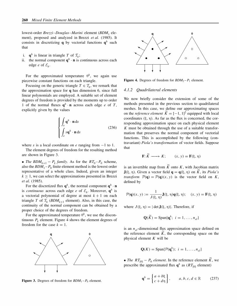
260 Mixed Finite Element Methods
lowest-order Brezzi–Douglas–Marini element (BDM1 ele-ment), proposed and analyzed in Brezzi et al. (1985). Itconsists in discretizing q by vectorial functions qh suchthat
i. qh is linear in triangle T of Th;ii. the normal component qh · n is continuous across each
edge e of Eh.
For the approximated temperature θh, we again usepiecewise constant functions on each triangle.
Focusing on the generic triangle T ∈ Th, we remark thatthe approximation space for q has dimension 6, since fulllinear polynomials are employed. A suitable set of elementdegrees of freedom is provided by the moments up to order1 of the normal fluxes qh · n across each edge e of T ,explicitly given by the values
∫e
qh · n ds∫e
sqh · n ds
(236)
where s is a local coordinate on e ranging from −1 to 1.The element degrees of freedom for the resulting method
are shown in Figure 3.
• The BDMk+1 − Pk family. As for the RT0 –P0 scheme,also the BDM1 –P0 finite element method is the lowest orderrepresentative of a whole class. Indeed, given an integerk ≥ 1, we can select the approximations presented in Brezziet al. (1985).
For the discretized flux qh, the normal component qh · nis continuous across each edge e of Eh. Moreover, qh isa vectorial polynomial of degree at most k + 1 on eachtriangle T of Th (BDMk+1 element). Also, in this case, thecontinuity of the normal component can be obtained by aproper choice of the degrees of freedom.
For the approximated temperature θh, we use the discon-tinuous Pk element. Figure 4 shows the element degrees offreedom for the case k = 1.
q θ
Figure 3. Degrees of freedom for BDM1 –P0 element.
q θ
Figure 4. Degrees of freedom for BDM2 –P1 element.
4.1.2 Quadrilateral elements
We now briefly consider the extension of some of themethods presented in the previous section to quadrilateralmeshes. In this case, we define our approximating spaceson the reference element K = [−1, 1]2 equipped with localcoordinates (ξ, η). As far as the flux is concerned, the cor-responding approximation space on each physical elementK must be obtained through the use of a suitable transfor-mation that preserves the normal component of vectorialfunctions. This is accomplished by the following (con-travariant) Piola’s transformation of vector fields. Supposethat
F: K −−−→ K; (x, y) = F(ξ, η)
is an invertible map from K onto K , with Jacobian matrixJ(ξ, η). Given a vector field q = q(ξ, η) on K , its Piola’stransform P(q) = P(q)(x, y) is the vector field on K ,defined by
P(q)(x, y) := 1
J (ξ, η)J(ξ, η)q(ξ, η); (x, y) = F(ξ, η)
where J (ξ, η) = | det J(ξ, η)|. Therefore, if
Q(K) = Span{qhi ; i = 1, . . . , nel}
is an nel-dimensional flux approximation space defined onthe reference element K , the corresponding space on thephysical element K will be
Q(K) = Span{P(qhi ); i = 1, . . . , nel}
• The RT[0] − P0 element. In the reference element K , weprescribe the approximated flux qh as (RT[0] element)
qh ={
a + bξ
c + dη
}, a, b, c, d ∈ R (237)
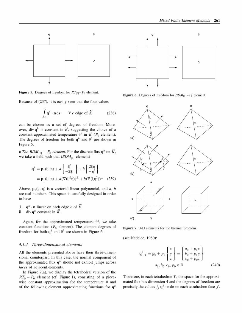
Mixed Finite Element Methods 261
q θ
Figure 5. Degrees of freedom for RT[0] –P0 element.
Because of (237), it is easily seen that the four values∫e
qh · n ds ∀ e edge of K (238)
can be chosen as a set of degrees of freedom. More-over, div qh is constant in K , suggesting the choice of aconstant approximated temperature θh in K (P0 element).The degrees of freedom for both qh and θh are shown inFigure 5.
• The BDM[1] − P0 element. For the discrete flux qh on K ,we take a field such that (BDM[1] element)
qh = p1(ξ, η) + a
{ξ2
−2ξη
}+ b
{2ξη
−η2
}= p1(ξ, η) + a(∇(ξ2η))⊥ + b(∇(ξη2))⊥ (239)
Above, p1(ξ, η) is a vectorial linear polynomial, and a, b
are real numbers. This space is carefully designed in orderto have
i. qh · n linear on each edge e of K .ii. div qh constant in K .
Again, for the approximated temperature θh, we takeconstant functions (P0 element). The element degrees offreedom for both qh and θh are shown in Figure 6.
4.1.3 Three-dimensional elements
All the elements presented above have their three-dimen-sional counterpart. In this case, the normal component ofthe approximated flux qh should not exhibit jumps acrossfaces of adjacent elements.
In Figure 7(a), we display the tetrahedral version of theRT0 − P0 element (cf. Figure 1), consisting of a piece-wise constant approximation for the temperature θ andof the following element approximating functions for qh
q θ
Figure 6. Degrees of freedom for BDM[1] –P0 element.
(a)
(b)
(c)
q θ
Figure 7. 3-D elements for the thermal problem.
(see Nedelec, 1980):
qh|T = p0 + p0
x
y
z
=
a0 + p0x
b0 + p0y
c0 + p0z
a0, b0, c0, p0 ∈ R (240)
Therefore, in each tetrahedron T , the space for the approxi-mated flux has dimension 4 and the degrees of freedom areprecisely the values
∫f
qh · n dσ on each tetrahedron face f .
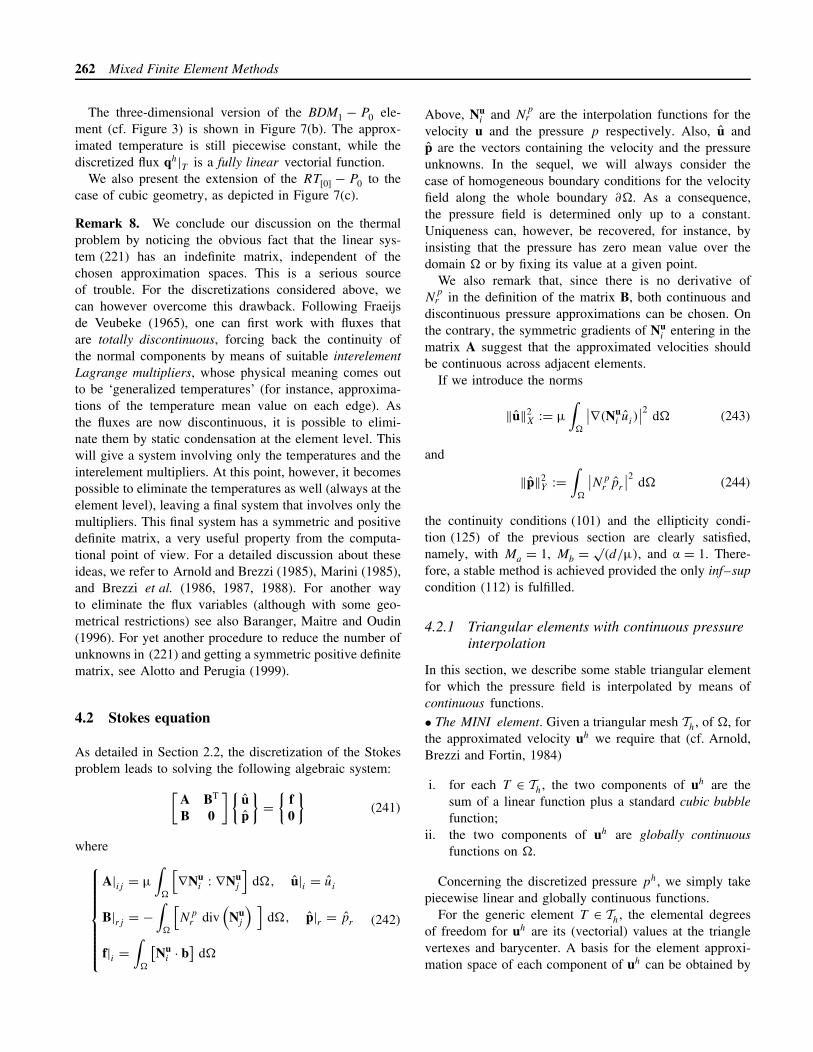
262 Mixed Finite Element Methods
The three-dimensional version of the BDM1 − P0 ele-ment (cf. Figure 3) is shown in Figure 7(b). The approx-imated temperature is still piecewise constant, while thediscretized flux qh|T is a fully linear vectorial function.
We also present the extension of the RT[0] − P0 to thecase of cubic geometry, as depicted in Figure 7(c).
Remark 8. We conclude our discussion on the thermalproblem by noticing the obvious fact that the linear sys-tem (221) has an indefinite matrix, independent of thechosen approximation spaces. This is a serious sourceof trouble. For the discretizations considered above, wecan however overcome this drawback. Following Fraeijsde Veubeke (1965), one can first work with fluxes thatare totally discontinuous, forcing back the continuity ofthe normal components by means of suitable interelementLagrange multipliers, whose physical meaning comes outto be ‘generalized temperatures’ (for instance, approxima-tions of the temperature mean value on each edge). Asthe fluxes are now discontinuous, it is possible to elimi-nate them by static condensation at the element level. Thiswill give a system involving only the temperatures and theinterelement multipliers. At this point, however, it becomespossible to eliminate the temperatures as well (always at theelement level), leaving a final system that involves only themultipliers. This final system has a symmetric and positivedefinite matrix, a very useful property from the computa-tional point of view. For a detailed discussion about theseideas, we refer to Arnold and Brezzi (1985), Marini (1985),and Brezzi et al. (1986, 1987, 1988). For another wayto eliminate the flux variables (although with some geo-metrical restrictions) see also Baranger, Maitre and Oudin(1996). For yet another procedure to reduce the number ofunknowns in (221) and getting a symmetric positive definitematrix, see Alotto and Perugia (1999).
4.2 Stokes equation
As detailed in Section 2.2, the discretization of the Stokesproblem leads to solving the following algebraic system:[
A BT
B 0
]{up
}={
f0
}(241)
where
A|ij = µ
∫�
[∇Nu
i : ∇Nuj
]d�, u|i = ui
B|rj = −∫
�
[Np
r div(
Nuj
) ]d�, p|r = pr
f|i =∫
�
[Nu
i · b]
d�
(242)
Above, Nui and N
pr are the interpolation functions for the
velocity u and the pressure p respectively. Also, u andp are the vectors containing the velocity and the pressureunknowns. In the sequel, we will always consider thecase of homogeneous boundary conditions for the velocityfield along the whole boundary ∂�. As a consequence,the pressure field is determined only up to a constant.Uniqueness can, however, be recovered, for instance, byinsisting that the pressure has zero mean value over thedomain � or by fixing its value at a given point.
We also remark that, since there is no derivative ofN
pr in the definition of the matrix B, both continuous and
discontinuous pressure approximations can be chosen. Onthe contrary, the symmetric gradients of Nu
i entering in thematrix A suggest that the approximated velocities shouldbe continuous across adjacent elements.
If we introduce the norms
‖u‖2X := µ
∫�
∣∣∇(Nui ui)
∣∣2 d� (243)
and
‖p‖2Y :=
∫�
∣∣Npr pr
∣∣2 d� (244)
the continuity conditions (101) and the ellipticity condi-tion (125) of the previous section are clearly satisfied,namely, with Ma = 1, Mb = √
(d/µ), and α = 1. There-fore, a stable method is achieved provided the only inf–supcondition (112) is fulfilled.
4.2.1 Triangular elements with continuous pressureinterpolation
In this section, we describe some stable triangular elementfor which the pressure field is interpolated by means ofcontinuous functions.• The MINI element. Given a triangular mesh Th, of �, forthe approximated velocity uh we require that (cf. Arnold,Brezzi and Fortin, 1984)
i. for each T ∈ Th, the two components of uh are thesum of a linear function plus a standard cubic bubblefunction;
ii. the two components of uh are globally continuousfunctions on �.
Concerning the discretized pressure ph, we simply takepiecewise linear and globally continuous functions.
For the generic element T ∈ Th, the elemental degreesof freedom for uh are its (vectorial) values at the trianglevertexes and barycenter. A basis for the element approxi-mation space of each component of uh can be obtained by
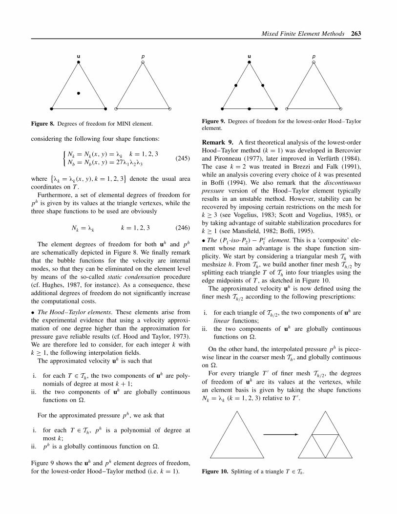
Mixed Finite Element Methods 263
u p
Figure 8. Degrees of freedom for MINI element.
considering the following four shape functions:{Nk = Nk(x, y) = λk k = 1, 2, 3Nb = Nb(x, y) = 27λ1λ2λ3
(245)
where{λk = λk(x, y), k = 1, 2, 3
}denote the usual area
coordinates on T .Furthermore, a set of elemental degrees of freedom for
ph is given by its values at the triangle vertexes, while thethree shape functions to be used are obviously
Nk = λk k = 1, 2, 3 (246)
The element degrees of freedom for both uh and ph
are schematically depicted in Figure 8. We finally remarkthat the bubble functions for the velocity are internalmodes, so that they can be eliminated on the element levelby means of the so-called static condensation procedure(cf. Hughes, 1987, for instance). As a consequence, theseadditional degrees of freedom do not significantly increasethe computational costs.
• The Hood–Taylor elements. These elements arise fromthe experimental evidence that using a velocity approxi-mation of one degree higher than the approximation forpressure gave reliable results (cf. Hood and Taylor, 1973).We are therefore led to consider, for each integer k withk ≥ 1, the following interpolation fields.
The approximated velocity uh is such that
i. for each T ∈ Th, the two components of uh are poly-nomials of degree at most k + 1;
ii. the two components of uh are globally continuousfunctions on �.
For the approximated pressure ph, we ask that
i. for each T ∈ Th, ph is a polynomial of degree atmost k;
ii. ph is a globally continuous function on �.
Figure 9 shows the uh and ph element degrees of freedom,for the lowest-order Hood–Taylor method (i.e. k = 1).
u p
Figure 9. Degrees of freedom for the lowest-order Hood–Taylorelement.
Remark 9. A first theoretical analysis of the lowest-orderHood–Taylor method (k = 1) was developed in Bercovierand Pironneau (1977), later improved in Verfurth (1984).The case k = 2 was treated in Brezzi and Falk (1991),while an analysis covering every choice of k was presentedin Boffi (1994). We also remark that the discontinuouspressure version of the Hood–Taylor element typicallyresults in an unstable method. However, stability can berecovered by imposing certain restrictions on the mesh fork ≥ 3 (see Vogelius, 1983; Scott and Vogelius, 1985), orby taking advantage of suitable stabilization procedures fork ≥ 1 (see Mansfield, 1982; Boffi, 1995).• The (P1-iso-P2) − P c
1 element. This is a ‘composite’ ele-ment whose main advantage is the shape function sim-plicity. We start by considering a triangular mesh Th withmeshsize h. From Th, we build another finer mesh Th/2 bysplitting each triangle T of Th into four triangles using theedge midpoints of T , as sketched in Figure 10.
The approximated velocity uh is now defined using thefiner mesh Th/2 according to the following prescriptions:
i. for each triangle of Th/2, the two components of uh arelinear functions;
ii. the two components of uh are globally continuousfunctions on �.
On the other hand, the interpolated pressure ph is piece-wise linear in the coarser mesh Th, and globally continuouson �.
For every triangle T ′ of finer mesh Th/2, the degreesof freedom of uh are its values at the vertexes, whilean element basis is given by taking the shape functionsNk = λk (k = 1, 2, 3) relative to T ′.
Figure 10. Splitting of a triangle T ∈ Th.
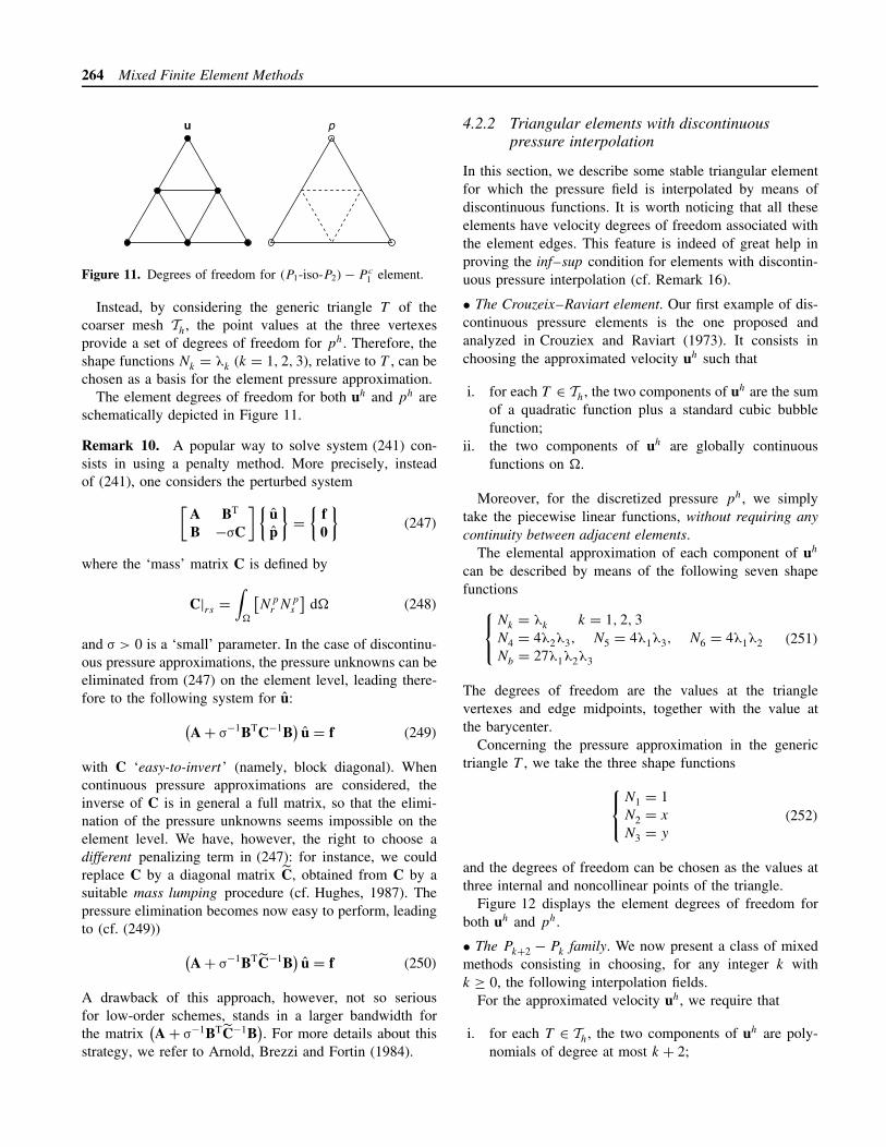
264 Mixed Finite Element Methods
u p
Figure 11. Degrees of freedom for (P1-iso-P2) − P c1 element.
Instead, by considering the generic triangle T of thecoarser mesh Th, the point values at the three vertexesprovide a set of degrees of freedom for ph. Therefore, theshape functions Nk = λk (k = 1, 2, 3), relative to T , can bechosen as a basis for the element pressure approximation.
The element degrees of freedom for both uh and ph areschematically depicted in Figure 11.
Remark 10. A popular way to solve system (241) con-sists in using a penalty method. More precisely, insteadof (241), one considers the perturbed system[
A BT
B −σC
]{up
}={
f0
}(247)
where the ‘mass’ matrix C is defined by
C|rs =∫
�
[Np
r Nps
]d� (248)
and σ > 0 is a ‘small’ parameter. In the case of discontinu-ous pressure approximations, the pressure unknowns can beeliminated from (247) on the element level, leading there-fore to the following system for u:(
A + σ−1BTC−1B)
u = f (249)
with C ‘easy-to-invert’ (namely, block diagonal). Whencontinuous pressure approximations are considered, theinverse of C is in general a full matrix, so that the elimi-nation of the pressure unknowns seems impossible on theelement level. We have, however, the right to choose adifferent penalizing term in (247): for instance, we couldreplace C by a diagonal matrix C, obtained from C by asuitable mass lumping procedure (cf. Hughes, 1987). Thepressure elimination becomes now easy to perform, leadingto (cf. (249)) (
A + σ−1BTC−1B)
u = f (250)
A drawback of this approach, however, not so seriousfor low-order schemes, stands in a larger bandwidth forthe matrix
(A + σ−1BTC−1B
). For more details about this
strategy, we refer to Arnold, Brezzi and Fortin (1984).
4.2.2 Triangular elements with discontinuouspressure interpolation
In this section, we describe some stable triangular elementfor which the pressure field is interpolated by means ofdiscontinuous functions. It is worth noticing that all theseelements have velocity degrees of freedom associated withthe element edges. This feature is indeed of great help inproving the inf–sup condition for elements with discontin-uous pressure interpolation (cf. Remark 16).
• The Crouzeix–Raviart element. Our first example of dis-continuous pressure elements is the one proposed andanalyzed in Crouziex and Raviart (1973). It consists inchoosing the approximated velocity uh such that
i. for each T ∈ Th, the two components of uh are the sumof a quadratic function plus a standard cubic bubblefunction;
ii. the two components of uh are globally continuousfunctions on �.
Moreover, for the discretized pressure ph, we simplytake the piecewise linear functions, without requiring anycontinuity between adjacent elements.
The elemental approximation of each component of uh
can be described by means of the following seven shapefunctions
Nk = λk k = 1, 2, 3N4 = 4λ2λ3, N5 = 4λ1λ3, N6 = 4λ1λ2Nb = 27λ1λ2λ3
(251)
The degrees of freedom are the values at the trianglevertexes and edge midpoints, together with the value atthe barycenter.
Concerning the pressure approximation in the generictriangle T , we take the three shape functions
N1 = 1N2 = x
N3 = y
(252)
and the degrees of freedom can be chosen as the values atthree internal and noncollinear points of the triangle.
Figure 12 displays the element degrees of freedom forboth uh and ph.
• The Pk+2 − Pk family. We now present a class of mixedmethods consisting in choosing, for any integer k withk ≥ 0, the following interpolation fields.
For the approximated velocity uh, we require that
i. for each T ∈ Th, the two components of uh are poly-nomials of degree at most k + 2;
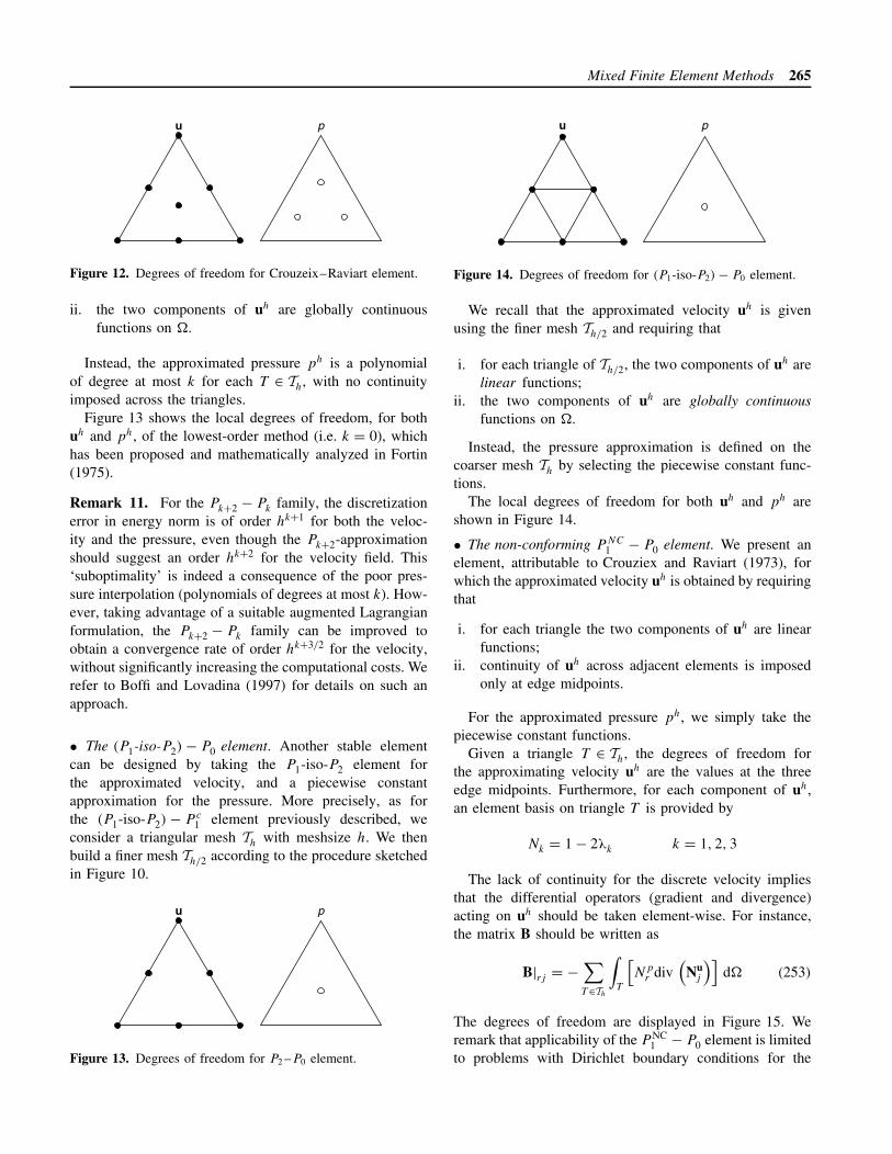
Mixed Finite Element Methods 265
u p
Figure 12. Degrees of freedom for Crouzeix–Raviart element.
ii. the two components of uh are globally continuousfunctions on �.
Instead, the approximated pressure ph is a polynomialof degree at most k for each T ∈ Th, with no continuityimposed across the triangles.
Figure 13 shows the local degrees of freedom, for bothuh and ph, of the lowest-order method (i.e. k = 0), whichhas been proposed and mathematically analyzed in Fortin(1975).
Remark 11. For the Pk+2 − Pk family, the discretizationerror in energy norm is of order hk+1 for both the veloc-ity and the pressure, even though the Pk+2-approximationshould suggest an order hk+2 for the velocity field. This‘suboptimality’ is indeed a consequence of the poor pres-sure interpolation (polynomials of degrees at most k). How-ever, taking advantage of a suitable augmented Lagrangianformulation, the Pk+2 − Pk family can be improved toobtain a convergence rate of order hk+3/2 for the velocity,without significantly increasing the computational costs. Werefer to Boffi and Lovadina (1997) for details on such anapproach.
• The (P1-iso-P2) − P0 element. Another stable elementcan be designed by taking the P1-iso-P2 element forthe approximated velocity, and a piecewise constantapproximation for the pressure. More precisely, as forthe (P1-iso-P2) − P c
1 element previously described, weconsider a triangular mesh Th with meshsize h. We thenbuild a finer mesh Th/2 according to the procedure sketchedin Figure 10.
u p
Figure 13. Degrees of freedom for P2 –P0 element.
u p
Figure 14. Degrees of freedom for (P1-iso-P2) − P0 element.
We recall that the approximated velocity uh is givenusing the finer mesh Th/2 and requiring that
i. for each triangle of Th/2, the two components of uh arelinear functions;
ii. the two components of uh are globally continuousfunctions on �.
Instead, the pressure approximation is defined on thecoarser mesh Th by selecting the piecewise constant func-tions.
The local degrees of freedom for both uh and ph areshown in Figure 14.
• The non-conforming P NC1 − P0 element. We present an
element, attributable to Crouziex and Raviart (1973), forwhich the approximated velocity uh is obtained by requiringthat
i. for each triangle the two components of uh are linearfunctions;
ii. continuity of uh across adjacent elements is imposedonly at edge midpoints.
For the approximated pressure ph, we simply take thepiecewise constant functions.
Given a triangle T ∈ Th, the degrees of freedom forthe approximating velocity uh are the values at the threeedge midpoints. Furthermore, for each component of uh,an element basis on triangle T is provided by
Nk = 1 − 2λk k = 1, 2, 3
The lack of continuity for the discrete velocity impliesthat the differential operators (gradient and divergence)acting on uh should be taken element-wise. For instance,the matrix B should be written as
B|rj = −∑T ∈Th
∫T
[Np
r div(
Nuj
)]d� (253)
The degrees of freedom are displayed in Figure 15. Weremark that applicability of the P NC
1 − P0 element is limitedto problems with Dirichlet boundary conditions for the

266 Mixed Finite Element Methods
u p
Figure 15. Degrees of freedom for P NC1 − P0 element.
displacement field imposed on the whole ∂�. For othersituations (e.g. a pure traction problem), the scheme exhibitsspurious mechanisms, because of its inability to controlthe rigid body rotations (cf. Hughes, 1987). Two stablemodifications of the P NC
1 − P0 element have been proposedand analyzed in Falk (1991) and, recently, in Hansbo andLarson (2003).
4.2.3 Quadrilateral elements
Many of the triangular elements presented above have theirquadrilateral counterpart. As an example, we here showthe so-called Q2 − Qc
1 element, which is the quadrilat-eral version of the lowest-order Hood–Taylor element (cf.Figure 9). Accordingly, the velocity is approximated bybiquadratic and continuous functions, while the pressure isdiscretized by means of bilinear and continuous functions,as depicted in Figure 16.
Another very popular scheme is the Q2 − P1 element,based on the same approximated velocities as before.Instead, the interpolating functions for the pressure arepiecewise linear, without requiring any continuity acrossthe elements. The local degrees of freedom are displayedin Figure 17.
4.2.4 Three-dimensional elements
Several elements previously described extend to thecase of three-dimensional problems. In Figure 18(a), weshow a continuous pressure tetrahedral element, which isnothing but the 3-D version of the MINI element (cf.
u p
Figure 16. Degrees of freedom for Q2 − Qc1 element.
u p
Figure 17. Degrees of freedom for Q2 − P1 element.
Figure 8). Also, the non-conforming P NC1 − P0 element
(cf. Figure 15) has its three-dimensional counterpart, asdepicted in Figure 18(b). We remark that the degrees offreedom for the velocity are given by the values at thebarycenter of each tetrahedron face. Figure 18(c) shows anexample of cubic element, which is exactly the 3-D versionof the popular Q2 − P1 element (cf. Figure 17).
Finally, we refer to Stenberg (1987) for the analysis,based on the so-called macroelement technique introducedin Stenberg (1984), of the lowest-order 3-D Hood–Taylormethod, and to Boffi (1997) for the higher-order case.
4.2.5 Stabilized formulations
From the above discussion, it should be clear that the fulfill-ment of the inf–sup condition requires a careful choice ofthe discretization spaces for the velocity and the pressure.A first strategy to obtain stability has been to derive the
u p
(a)
(b)
(c)
Figure 18. 3-D Stokes elements.
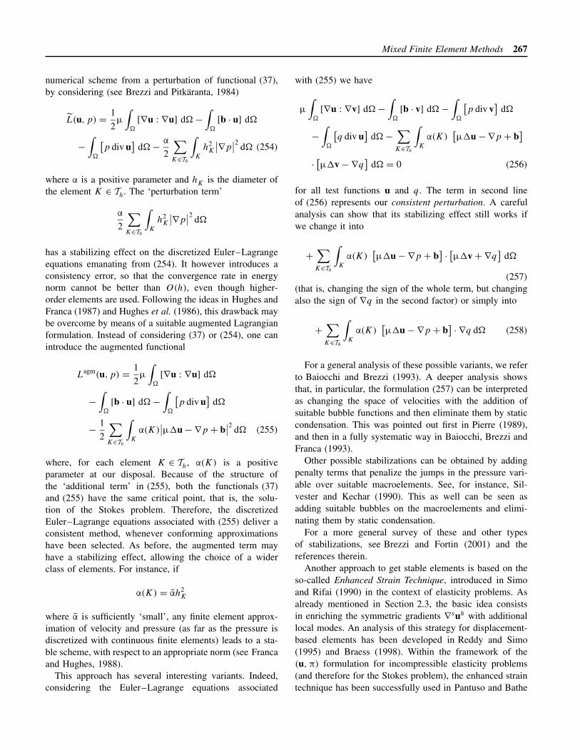
Mixed Finite Element Methods 267
numerical scheme from a perturbation of functional (37),by considering (see Brezzi and Pitkaranta, 1984)
L(u, p) = 1
2µ
∫�
[∇u : ∇u] d� −∫
�
[b · u] d�
−∫
�
[p div u
]d� − α
2
∑K∈Th
∫K
h2K
∣∣∇p∣∣2 d� (254)
where α is a positive parameter and hK is the diameter ofthe element K ∈ Th. The ‘perturbation term’
α
2
∑K∈Th
∫K
h2K
∣∣∇p∣∣2 d�
has a stabilizing effect on the discretized Euler–Lagrangeequations emanating from (254). It however introduces aconsistency error, so that the convergence rate in energynorm cannot be better than O(h), even though higher-order elements are used. Following the ideas in Hughes andFranca (1987) and Hughes et al. (1986), this drawback maybe overcome by means of a suitable augmented Lagrangianformulation. Instead of considering (37) or (254), one canintroduce the augmented functional
Lagm(u, p) = 1
2µ
∫�
[∇u : ∇u] d�
−∫
�
[b · u] d� −∫
�
[p div u
]d�
− 1
2
∑K∈Th
∫K
α(K)∣∣µ�u − ∇p + b
∣∣2 d� (255)
where, for each element K ∈ Th, α(K) is a positiveparameter at our disposal. Because of the structure ofthe ‘additional term’ in (255), both the functionals (37)and (255) have the same critical point, that is, the solu-tion of the Stokes problem. Therefore, the discretizedEuler–Lagrange equations associated with (255) deliver aconsistent method, whenever conforming approximationshave been selected. As before, the augmented term mayhave a stabilizing effect, allowing the choice of a widerclass of elements. For instance, if
α(K) = αh2K
where α is sufficiently ‘small’, any finite element approx-imation of velocity and pressure (as far as the pressure isdiscretized with continuous finite elements) leads to a sta-ble scheme, with respect to an appropriate norm (see Francaand Hughes, 1988).
This approach has several interesting variants. Indeed,considering the Euler–Lagrange equations associated
with (255) we have
µ
∫�
[∇u : ∇v] d� −∫
�
[b · v] d� −∫
�
[p div v
]d�
−∫
�
[q div u
]d� −
∑K∈Th
∫K
α(K)[µ�u − ∇p + b
]· [µ�v − ∇q
]d� = 0 (256)
for all test functions u and q. The term in second lineof (256) represents our consistent perturbation. A carefulanalysis can show that its stabilizing effect still works ifwe change it into
+∑K∈Th
∫K
α(K)[µ�u − ∇p + b
] · [µ�v + ∇q]
d�
(257)
(that is, changing the sign of the whole term, but changingalso the sign of ∇q in the second factor) or simply into
+∑K∈Th
∫K
α(K)[µ�u − ∇p + b
] · ∇q d� (258)
For a general analysis of these possible variants, we referto Baiocchi and Brezzi (1993). A deeper analysis showsthat, in particular, the formulation (257) can be interpretedas changing the space of velocities with the addition ofsuitable bubble functions and then eliminate them by staticcondensation. This was pointed out first in Pierre (1989),and then in a fully systematic way in Baiocchi, Brezzi andFranca (1993).
Other possible stabilizations can be obtained by addingpenalty terms that penalize the jumps in the pressure vari-able over suitable macroelements. See, for instance, Sil-vester and Kechar (1990). This as well can be seen asadding suitable bubbles on the macroelements and elimi-nating them by static condensation.
For a more general survey of these and other typesof stabilizations, see Brezzi and Fortin (2001) and thereferences therein.
Another approach to get stable elements is based on theso-called Enhanced Strain Technique, introduced in Simoand Rifai (1990) in the context of elasticity problems. Asalready mentioned in Section 2.3, the basic idea consistsin enriching the symmetric gradients ∇suh with additionallocal modes. An analysis of this strategy for displacement-based elements has been developed in Reddy and Simo(1995) and Braess (1998). Within the framework of the(u,π) formulation for incompressible elasticity problems(and therefore for the Stokes problem), the enhanced straintechnique has been successfully used in Pantuso and Bathe
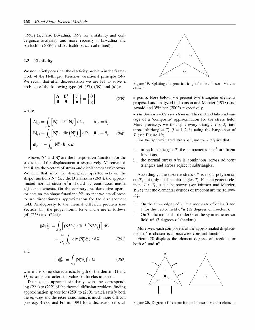
268 Mixed Finite Element Methods
(1995) (see also Lovadina, 1997 for a stability and con-vergence analysis), and more recently in Lovadina andAuricchio (2003) and Auricchio et al. (submitted).
4.3 Elasticity
We now briefly consider the elasticity problem in the frame-work of the Hellinger–Reissner variational principle (59).We recall that after discretization we are led to solve aproblem of the following type (cf. (57), (58), and (61)):[
A BT
B 0
]{σ
u
}={
0g
}(259)
where
A|ij =∫
�
[Nσ
i : D−1Nσ
j
]d�, σ|j = σj
B|rj =∫
�
[Nu
r · div(
Nσj
) ]d�, u|r = ur
g|r = −∫
�
[Nu
r · b]
d�
(260)
Above, Nσi and Nu
r are the interpolation functions for thestress σ and the displacement u respectively. Moreover, σ
and u are the vectors of stress and displacement unknowns.We note that since the divergence operator acts on theshape functions Nσ
i (see the B matrix in (260)), the approx-imated normal stress σhn should be continuous acrossadjacent elements. On the contrary, no derivative opera-tor acts on the shape functions Nu
r , so that we are allowedto use discontinuous approximation for the displacementfield. Analogously to the thermal diffusion problem (seeSection 4.1), the proper norms for σ and u are as follows(cf. (223) and (224)):
‖σ‖2X :=
∫�
[(Nσ
i σi
): D
−1(
Nσj σj
)]d�
+ �2
D∗
∫�
|div (Nσi σi)|2 d� (261)
and
‖u‖2Y :=
∫�
|Nur ur |2 d� (262)
where � is some characteristic length of the domain � andD∗ is some characteristic value of the elastic tensor.
Despite the apparent similarity with the correspond-ing (221) to (222) of the thermal diffusion problem, findingapproximation spaces for (259) to (260), which satisfy boththe inf–sup and the elker conditions, is much more difficult(see e.g. Brezzi and Fortin, 1991 for a discussion on such
T1 T3
T2
Figure 19. Splitting of a generic triangle for the Johnson–Mercierelement.
a point). Here below, we present two triangular elementsproposed and analyzed in Johnson and Mercier (1978) andArnold and Winther (2002) respectively.
• The Johnson–Mercier element. This method takes advan-tage of a ‘composite’ approximation for the stress field.More precisely, we first split every triangle T ∈ Th intothree subtriangles Ti (i = 1, 2, 3) using the barycenter ofT (see Figure 19).
For the approximated stress σh, we then require that
i. in each subtriangle Ti the components of σh are linearfunctions;
ii. the normal stress σhn is continuous across adjacenttriangles and across adjacent subtriangles.
Accordingly, the discrete stress σh is not a polynomialon T , but only on the subtriangles Ti . For the generic ele-ment T ∈ Th, it can be shown (see Johnson and Mercier,1978) that the elemental degrees of freedom are the follow-ing.
i. On the three edges of T : the moments of order 0 and1 for the vector field σhn (12 degrees of freedom);
ii. On T : the moments of order 0 for the symmetric tensorfield σh (3 degrees of freedom).
Moreover, each component of the approximated displace-ment uh is chosen as a piecewise constant function.
Figure 20 displays the element degrees of freedom forboth σh and uh.
σ u
Figure 20. Degrees of freedom for the Johnson–Mercier element.
Mixed Finite Element Methods 269
• The Arnold–Winther element. This triangular element hasbeen recently proposed and analyzed in Arnold and Winther(2002), where higher-order schemes are also considered.For the approximated stress σh, we impose that
i. on each T ∈ Th, σh is a symmetric tensor whosecomponents are cubic functions, but div σh is a linearvector field;
ii. the normal stress σhn is continuous across adjacenttriangles.
For each element T ∈ Th, the approximation space for thestress field has dimension 24 and the elemental degrees offreedom can be chosen as follows (see Arnold and Winther,2002):
i. the values of the symmetric tensor field σh at thevertices of T (9 degrees of freedom);
ii. the moments of order 0 and 1 for the vector field σhnon each edge of T (12 degrees of freedom);
iii. the moment of order 0 for σh on T (3 degrees offreedom).
Furthermore, the components of the approximated dis-placement uh are piecewise linear functions, without requir-ing any continuity across adjacent elements.
In Figure 21, the element degrees of freedom for bothσh and uh are schematically depicted.
Remark 12. Other methods exploiting ‘composite’ app-roximations as for the Johnson–Mercier element havebeen proposed and analyzed in Arnold, Douglas and Gupta(1984).
Following the ideas in Fraeijs de Veubeke (1975), adifferent strategy to obtain reliable schemes for the elas-ticity problem in the context of the Hellinger–Reissnervariational principle consists in the use of unsymmetricapproximated stresses. Symmetry is then enforced back ina weak form by the introduction of a suitable Lagrangemultiplier. We refer to Amara and Thomas (1979), Arnold,Brezzi and Douglas (1984), Brezzi et al. (1986), and Sten-berg (1988) for the details on such an approach.
σ u
Figure 21. Degrees of freedom for the Arnold–Winther element.
5 TECHNIQUES FOR PROVING THEINF–SUP CONDITION
In this section we give some hints on how to prove theinf–sup condition (118). We also show how the stabilityresults detailed in Section 3 can be exploited to obtainerror estimates. We focus on the Stokes problem, as arepresentative example, but analogous strategies can beapplied to analyze most of the methods considered inSection 4.
We begin recalling (cf. (38)) that a weak form of theStokes problem with homogeneous boundary conditions forthe velocity consists in finding (u, p) such that
µ
∫�
[(∇δu) : ∇u] d� −∫
�
[div (δu) p
]d�
=∫
�
[δu · b] d�∫�
[δp div u
]d� = 0
(263)
for any admissible velocity variation δu and any admissiblepressure variation δp. On the other hand, as detailed inSection 4.2, the discretized problem consists in solving[
A BT
B 0
]{up
}={
f0
}(264)
where
A|ij = µ
∫�
[∇Nu
i : ∇Nuj
]d�, u|i = ui
B|rj = −∫
�
[Np
r div(
Nuj
) ]d�, p|r = pr
f|i =∫
�
[Nu
i · b]
d�
(265)
with i, j = 1, . . . , n and r = 1, . . . , m.With our notation for the Stokes problem, the inf–sup
condition in its equivalent form (119) consists in requiringthe existence of a positive constant β, independent of h,such that
∀ q ∈ Y supz∈X\{0}
zTBTq‖z‖X
≥ β‖q‖Y (266)
where X ≡ Rn and Y ≡ R
m.Moreover, in what follows, we need to introduce the
space X for vectorial functions v, defined by
X ={
v : v|∂� = 0, ‖v‖2X := µ
∫�
|∇v|2 d� < +∞}
(267)
270 Mixed Finite Element Methods
and the space Y for scalar functions q, defined by
Y ={q : ‖q‖2
Y :=∫
�
|q|2 d� < +∞}
(268)
Remark 13. It is worth noticing that, whenever anapproximated velocity uh = Nu
i ui is considered, the follow-ing holds (cf. (243))
‖u‖X =(µ
∫�
|∇Nui ui |2 d�
)1/2
= ‖uh‖X (269)
Therefore, the X-norm we have tailored for vector u ∈ Xcoincides with the X-norm of the reconstructed function uh.Similarly (cf. (244)), if ph = N
pr pr , we have
‖p‖Y =(∫
�
|Npr pr |2 d�
)1/2
= ‖ph‖Y (270)
5.1 Checking the inf–sup condition
As already mentioned, a rigorous proof of the inf–supcondition is typically a difficult task, mainly because severaltechnical mathematical problems have to be overcome.In this section, we present two of the most powerfultools for proving the inf–sup property. The first technique(Fortin’s trick ) can be used, for instance, to study thestability of the P NC
1 − P0 element (cf. Figure 15) and theCrouzeix–Raviart element (cf. Figure 12), as we are goingto detail below. The second one (Verfurth’s trick ) can beapplied basically to all the approximations with continuouspressure and it will be exemplified by considering the MINIelement (cf. Figure 8).
Although we are aware that the subsequent analysis isnot completely satisfactory from the mathematical pointof view, it nonetheless highlights some of the basic ideasbehind the analysis of mixed finite element methods.
We first need to recall the following important theoremof functional analysis (see Ladyzhenskaya, 1969; Temam,1977, for instance).
Theorem 4. There exists a constant βc > 0 such that, for
every q ∈ Y with∫
�
q d� = 0, it holds
supv∈X\{0}
−∫
�
qdiv v d�
‖v‖X≥ βc‖q‖Y (271)
Remark 14. We remark that estimate (271) is nothing butthe infinite-dimensional version of the inf–sup conditionwritten in its equivalent form (119).
5.1.1 Fortin’s trick
The next result provides a criterion for proving the inf–supcondition, called Fortin’s trick (see Fortin, 1977) or, moreprecisely, Fortin’s trick applied to the Stokes problem.
Proposition 4. Suppose there exists a linear operator�h:X −−−→ X ≡ R
n such that
‖�hv‖X ≤ C�‖v‖X ∀ v ∈ X (272)
and
(�hv)TBTq = −∫
�
div v(Npr qr ) d� ∀ q ∈ Y ≡ R
m
(273)
with C� independent of h. Then it holds
∀ q ∈ Y supz∈X\{0}
zTBTq‖z‖X
≥ βc
C�
‖q‖Y (274)
that is, the inf–sup condition (266) is fulfilled with β =βc/C�.
Proof. Take any q ∈ Y. We notice that from Theorem 4and Remark 13, we get
supv∈X\{0}
−∫
�
div v(Npr qr ) d�
‖v‖X≥ βc‖Np
r qr‖Y = βc‖q‖Y
(275)
Therefore, from (273), we have
supv∈X\{0}
(�hv)TBTq‖v‖X
≥ βc‖q‖Y (276)
Using (272), from (276) it follows
supv∈X:�hv�=0
(�hv)TBTq
‖�hv‖X
≥ 1
C�
supv∈X\{0}
(�hv)TBTq‖v‖X
≥ βc
C�
‖q‖Y (277)
Since, obviously,{�hv; v ∈ X
} ⊆ X, from (277) weobtain
supz∈X\{0}
zTBTq‖z‖X
≥ supv∈X:�hv�=0
(�hv)TBTq
‖�hv‖X
≥ βc
C�
‖q‖Y �
(278)
We now apply Proposition 4 to the P NC1 − P0 element
and the Crouzeix–Raviart element, skipping, however, theproof of (272). In both cases, the strategy for building theoperator �h is the following:
Mixed Finite Element Methods 271
1. On each triangle T ∈ Th, we first define a suitable linearoperator �h,T : v �−−−→ �h,T v, valued in the space ofvelocity approximating functions on T , and satisfying∫
T
qhdiv (�h,T v) d� =∫
T
qhdiv v d� (279)
for every v ∈ X and every discrete pressure qh. Thiswill be done by using, in particular, the element degreesof freedom for the velocity approximation.
2. By assembling all the element contributions, we obtaina global linear operator
�h:
X −−−→ Span{Nu
i ; i = 1, . . . , n}
v �−−−→ �hv =∑T ∈Th
�h,T v = Nui vi
(280)
3. We finally define �h:X −−−→ Rn by setting
�hv = v if �hv = Nui vi (281)
that is, �hv returns the components of the func-tion �hv with respect to the global velocity basis{Nu
i ; i = 1, . . . , n}. From the definition of the matrixB, property (279), (280), and (281), it follows that con-dition (273) is satisfied.
• The P NC1 − P0 element. Fix T ∈ Th, and recall that any
approximated pressure qh is a constant function on T . Wewish to build �h,T in such a way that∫
T
qhdiv (�h,T v) d� =∫
T
qhdiv v d� (282)
From the divergence theorem, (282) can be alternativelywritten as∫
∂T
qh(�h,T v) · n ds =∫
∂T
qhv · n ds (283)
Denoting with Mk (k = 1, 2, 3) the midpoint of the edge ek,we define �h,T v as the unique (vectorial) linear functionsuch that
�h,T v(Mk) = 1
|ek|∫
ek
v ds k = 1, 2, 3 (284)
From the divergence theorem and the Midpoint rule, itfollows that∫
T
qhdiv (�1,T v) d� =∫
∂T
qh(�1,T v) · n ds
=∫
∂T
qhv · n ds =∫
T
qhdiv v d� (285)
for every constant function qh. It is now sufficient to definethe global linear operator �h as
�hv =∑T ∈Th
�h,T v = Nui vi
and the corresponding operator �h satisfies condition (273)(cf. also (253)).
• The Crouzeix–Raviart element. Fix T ∈ Th, and recallthat any approximated pressure qh is now a linear functionon T . Hence, qh can be uniquely decomposed as qh =q0 + q1, where q0 is a constant (the mean value of qh onT ), and q1 is a linear function having zero mean value. Wenow construct a linear operator �1,T : v �−−−→ �1,T v, where�1,T v is a quadratic vectorial polynomial such that∫
T
div (�1,T v) d� =∫
T
div v d� (286)
or, alternatively,∫∂T
(�1,T v) · n ds =∫
∂T
v · n ds (287)
Denoting with Vk (resp., Mk) the vertexes of T (resp., themidpoint of the edge ek), the Cavalieri–Simpson rule showsthat condition (287) holds if we set
�1,T v(Vk) = v(Vk) k = 1, 2, 3
�1,T v(Mk) = 3
2|ek|∫
ek
v ds − v(Vk1) + v(Vk2
)
4
k = 1, 2, 3
(288)
Above, we have denoted with Vk1and Vk2
the endpointsof side ek. So far, we have not used the bubble functionsavailable for the approximated velocity. We now use thesetwo additional degrees of freedom by defining vb,T (v) asthe unique vectorial bubble function such that∫
T
q1div vb,T (v) d� =∫
T
q1div (v − �1,T v) d� (289)
for every linear function q1 having zero mean value on T .We claim that if �h,T v = vb,T (v) + �1,T v, then∫
T
qhdiv (�h,T v) d� =∫
T
qhdiv v d� (290)
for every linear polynomial qh = q0 + q1. In fact, using(286), (289), and the obvious fact that
∫T
div vb,T (v)
272 Mixed Finite Element Methods
d� = 0, we have∫T
qhdiv (�h,T v) d� =∫
T
(q0 + q1)div (vb,T (v)
+ �1,T v) d� =∫
T
q0div (vb,T (v) + �1,T v) d�
+∫
T
q1div (vb,T (v) + �1,T v) d�
=∫
T
q0div (�1,T v) d� +∫
T
q1div v d�
=∫
T
q0div v d� +∫
T
q1div v d�
=∫
T
qhdiv v d� (291)
Hence, the operator �h arising from the global linearoperator
�hv =∑T ∈Th
(vb,T (v) + �1,T v
) = vb(v) + �1v = Nui vi
fulfills condition (273).
Remark 15. Conditions (288) reveal that the operator �1(built by means of the local contributions �1,T ) exploits,in particular, the point values of v at all the vertexes ofthe triangles in Th. However, this definition makes nosense for an arbitrary v ∈ X, since functions in X arenot necessarily continuous. To overcome this problem,one should define a more sophisticated operator �1 forinstance, taking advantage of an averaging procedure. Moreprecisely, one could define the function �1v as the uniquepiecewise quadratic polynomial such that �1v|∂� = 0 and
�1v(V ) = 1
Area(D(V ))
∫D(V )
v d�
�1v(M) = 3
2|eM |∫
eM
v ds − �1v(VM1) + �1v(VM2
)
4(292)
Above, V is any internal vertex of triangles in Th and D(V )
is the union of the triangles having V as a vertex. Moreover,eM is any internal edge having M as midpoint and VM1
, VM2
as endpoints. In this case, it is possible to prove that for theresulting �h, the very important property (272) holds withC� independent of h.
Remark 16. It is interesting to observe that condi-tion (283) and (287) suggest the following important factabout the discretization of the Stokes problem. Any rea-sonable discontinuous pressure approximation contains atleast all the piecewise constant functions: relations (283)
and (287) show that having some velocity degrees of free-dom associated with the triangle edges greatly helps inproving the inf–sup condition.
5.1.2 Verfurth’s trick
We now describe another technique for proving the inf–supcondition, which can be profitably used when elements withcontinuous pressure interpolation are considered: the so-called Verfurth’s trick (see Verfurth, 1984). We begin bynoting that, because of to the pressure continuity, it holds
zTBTq = −∫
�
(Np
r qr
)div
(Nu
j zj
)d�
=∫
�
(∇Npr qr) · Nu
j zj d� (293)
for every z ∈ X and q ∈ Y. In some cases, it is much easierto use the form (293) and prove a modified version of theinf–sup condition (266) with a norm for Y different fromthe one defined in (270) and involving the pressure gra-dients; see Bercovier and Pironneau (1977) and Glowinskiand Pironneau (1979). More precisely, given a mesh Th, weintroduce in Y the norm
‖p‖Y∗ :=∑
K∈Th
h2K
∫K
|∇Npr pr |2 d�
1/2
(294)
where hK denotes the diameter of the generic element K .The key point of Verfurth’s trick is a smart use of the
properties of interpolation operator in order to prove thatthe inf–sup condition with the norm Y∗ implies the usualone. Indeed, we have the following result.
Proposition 5. Suppose that
(H1) for every velocity v ∈ X there exists a discrete veloc-ity vI = Nu
j vIj such that∑
K∈Th
h−2K
∫K
|Nuj vI
j − v|2 d�
1/2
≤ c0‖v‖X (295)
‖vI‖X ≤ c1‖v‖X (296)
with c0, c1 independent of h and v;(H2) there exists a constant β∗ > 0 independent of h such
that
∀ q ∈ Y supz∈X\{0}
zTBTq‖z‖X
≥ β∗‖q‖Y∗ (297)
(i.e. the inf–sup condition holds with the modifiedY-norm (294)).
Mixed Finite Element Methods 273
Then the inf–sup condition (with respect to the originalnorm (270))
∀ q ∈ Y supz∈X\{0}
zTBTq‖z‖X
≥ β‖q‖Y (298)
is satisfied with β independent of h.
Proof. Given q ∈ Y, we observe that using (296) and (293)it holds
supz∈X\{0}
zTBTq‖z‖X
≥ supv∈X\{0}
vTI BTq
‖vI‖X
≥ supv∈X\{0}
vTI BTq
c1‖v‖X
= supv∈X\{0}
∫�
(∇Npr qr ) · Nu
j vIj d�
c1‖v‖X(299)
Furthermore, from Theorem 4, there exists w ∈ X suchthat
−∫
�
div w(Npr qr ) d�
‖w‖X=
∫�
(∇Npr qr) · w d�
‖w‖X≥ βc‖q‖Y
(300)
For such a velocity w and the corresponding discretevelocity wI = Nu
j wIj , we obviously have
supv∈X\{0}
∫�
(∇Npr qr ) · Nu
j vIj d�
c1‖v‖X≥
∫�
(∇Npr qr ) · Nu
j wIj d�
c1‖w‖X(301)
Subtracting and adding w, we obtain∫�
(∇Npr qr ) · Nu
j wIj d�
c1‖w‖X=
∫�
(∇Npr qr ) · (Nu
j wIj − w) d�
c1‖w‖X
+
∫�
(∇Npr qr ) · w d�
c1‖w‖X(302)
To treat the first term in the right-hand side of (302), weobserve that using (295) and recalling (294), we have
−∫
�
(∇Npr qr ) · (Nu
j wIj − w) d�
= −∑K∈Th
∫K
(∇Npr qr) · (Nu
j wIj − w) d�
= −∑K∈Th
∫K
hK(∇Npr qr ) · h−1
K (Nuj wI
j − w) d�
≤∑
K∈Th
h2K
∫K
|∇Npr qr |2 d�
1/2
×∑
K∈Th
h−2K
∫K
|Nuj wI
j − w|2 d�
1/2
≤ c0‖q‖Y∗‖w‖X (303)
which gives∫�
(∇Npr qr ) · (Nu
j wIj − w) d� ≥ −c0‖q‖Y∗‖w‖X (304)
Therefore, we get∫�
(∇Npr qr ) · (Nu
j wIj − w) d�
c1‖w‖X≥ −c0
c1‖q‖Y∗ (305)
For the second term in the right-hand side of (302), wenotice that (cf. (300))∫
�
(∇Npr qr ) · w d�
c1‖w‖X≥ βc
c1‖q‖Y (306)
Therefore, from (299), (301), (302), (305), and (306), weobtain
supz∈X\{0}
zTBTq‖z‖X
≥ βc
c1‖q‖Y − c0
c1‖q‖Y∗ (307)
We now multiply the modified inf–sup condition (297)by c0/(β∗c1) to get
c0
β∗c1sup
z∈X\{0}zTBTq‖z‖X
≥ c0
c1‖q‖Y∗ (308)
By adding (307) and (308), we finally have(1 + c0
β∗c1
)sup
z∈X\{0}zTBTq‖z‖X
≥ βc
c1‖q‖Y (309)
that is, the inf–sup condition (298) holds with β = (βc/c1)
(1 + (c0/β∗c1))−1.
Remark 17. We notice that hypothesis (H1) of Proposi-tion 5 is not very restrictive. Indeed, given a velocity v ∈ X,the corresponding vI can be chosen as a suitable discretevelocity interpolating v, and (295) and (296) are both sat-isfied basically for every element of practical interest (seee.g. Brezzi and Fortin, 1991 and Ciarlet, 1978 for moredetails).
274 Mixed Finite Element Methods
The Verfurth trick was originally applied to the Hood–Taylor element depicted in Figure 9 (see Verfurth, 1984),but it was soon recognized as a valuable instrument foranalyzing all continuous pressure elements. Here we showhow to use it for the analysis of the MINI element (whoseoriginal proof was given using Fortin’s trick in Arnold,Brezzi and Fortin, 1984).• The MINI element. We now give a hint on how to verifyhypothesis (H2) of Proposition 5 for the MINI element (cf.Figure 8).
For a generic q ∈ Y, we take its reconstructed discretepressure qh = N
pr qr . Since qh is a piecewise linear and
continuous function, it follows that ∇qh = ∇Npr qr is a
well-defined piecewise constant vector field. We now con-struct a discrete (bubble-type) velocity vh = Nu
j vj , definedon each triangle T ∈ Th as
vh = h2T bT ∇qh (310)
where bT is the usual cubic bubble (i.e. in area coordinates,bT = 27λ1λ2λ3). Recalling (293) and using (310), we thenobtain
vTBTq =∫
�
(∇Npr qr ) · Nu
j vj d� =∫
�
∇qh · vh d�
=∑T ∈Th
h2T
∫T
|∇Npr qr |2bT d� (311)
It is easy to show that for regular meshes (roughly: formeshes that do not contain ‘too thin’ elements, see e.g.Ciarlet, 1978 for a precise definition), there exists a constantC1 > 0, independent of h, such that
∀ T ∈ Th
∫T
|∇Npr qr |2bT d� ≥ C1
∫T
|∇Npr qr |2 d�
(312)
Therefore, from (311), (312), and (294) we get
vTBTq ≥ C1
∑T ∈Th
h2T
∫T
|∇Npr qr |2 d� = C1‖q‖2
Y∗ (313)
Furthermore, using standard scaling arguments (cf. Brezziand Fortin, 1991), it is possible to prove that there existsC2 > 0 independent of h such that
‖v‖X = ‖vh‖X ≤ C2
∑T ∈Th
h2T
∫T
|∇Npr qr |2 d�
1/2
= C2‖q‖Y∗ (314)
Hence, estimates (313) and (314) imply
vTBTq‖v‖X
≥ C1
C2‖q‖Y∗ (315)
and condition (297) then follows with β∗ = C1/C2, since
supz∈X\{0}
zTBTq‖z‖X
≥ vTBTq‖v‖X
(316)
5.2 Appendix — error estimates
In this brief Appendix, we present the guidelines to obtainerror estimates, once the stability conditions have beenestablished. We only consider the easiest case of conform-ing schemes (i.e. when the velocity is approximated bymeans of continuous functions). We refer to Brezzi (1974),Brezzi and Fortin (1991), and Braess (1997) for moredetails, as well as for the analysis of more complicatedsituations involving non-conforming approximations (suchas the P NC
1 − P0 element (cf. Figure 15)).Before proceeding, we recall that for the Stokes prob-
lem with our choices of norms, we have Ma = 1, Mb =√(d/µ), and α = 1, no matter what the approximations
of velocity and pressure are. However, in the subsequentdiscussion, we will not substitute these values into the esti-mates, in order to facilitate the extension of the analysisto other problems. We also notice that, on the contrary,the relevant constant β does depend on the choice of theinterpolating functions. We have the following result.
Theorem 5. Let (u, p) be the solution of problem (263)and suppose there exist discrete velocity and pressure
uI = Nui u
Ii , pI = Np
r pIr (317)
such that
‖u − uI‖X ≤ Chku , ku > 0 (318)
‖p − pI‖Y ≤ Chkp , kp > 0 (319)
If (u, p) is the solution of the discrete problem (264), then,setting uh = Nu
i ui and ph = Npr pr , it holds
‖u − uh‖X + ‖p − ph‖Y ≤ Chk (320)
with k = min{ku, kp}.
Proof. For uI and pI as in (317), we set uI = (uIi )
ni=1 ∈ X
and pI = (pIr )
mr=1 ∈ Y. Taking into account that{
up
}is the solution of the discretized problem (264), we obtainthat {
u − uI
p − pI
}
Mixed Finite Element Methods 275
solves[A BT
B 0
]{u − uI
p − pI
}={
f − AuI − BTpI
−BuI
}(321)
Choosing as (admissible) velocity and pressure variationsthe interpolating shape functions, from (263), we have
f|i = µ
∫�
∇Nui : ∇u d� −
∫�
div (Nui )p d�
i = 1, . . . , n (322)
and ∫�
Nps div u d� = 0 s = 1, . . . , m (323)
Hence, system (321) may be written as[A BT
B 0
]{u − uI
p − pI
}={
fg
}(324)
where
f|i := µ
∫�
∇Nui : ∇ (u − uI
)d�
−∫
�
div (Nui )(p − pI
)d� i = 1, . . . , n
(325)
and
g|r := −∫
�
Npr div (u − uI ) d� r = 1, . . . , m (326)
Applying Theorem 1, we thus obtain
‖u − uI‖X ≤ 1
α‖f‖F + M
1/2a
α1/2β‖g‖G (327)
‖p − pI‖Y ≤(
1
β+ M
1/2a
α1/2β
)‖f‖F + Ma
β2‖g‖G (328)
We proceed by estimating the dual norms ‖f‖F and ‖g‖G.Since for every v = (vi)
ni=1,
vTf = µ
∫�
∇ (Nui vi
): ∇ (u − uI
)d�
−∫
�
div (Nui vi)
(p − pI
)d� ≤ Ma‖v‖X‖u − uI‖X
+ Mb‖v‖X‖p − pI‖Y (329)
we obtain
vTf‖v‖X
≤ Ma‖u − uI‖X + Mb‖p − pI‖Y (330)
which gives (cf. the dual norm definition (104))
‖f‖F ≤ Ma‖u − uI‖X + Mb‖p − pI‖Y (331)
Analogously, for every q = (qr )mr=1, we get
qTg = −∫
�
(Np
r qr
)div (u − uI ) d� ≤ Mb‖q‖Y‖u − uI‖X
(332)
and therefore we have
‖g‖G ≤ Mb‖u − uI‖X (333)
From (327), (328), (331), and (333) we have
‖u − uI‖X ≤(
Ma
α+ M
1/2a Mb
α1/2β
)‖u − uI‖X
+ Mb
α‖p − pI‖Y (334)
‖p − pI‖Y ≤(
Ma
β+ M
3/2a
α1/2β+ MaMb
β2
)‖u − uI‖X
+ Mb
(1
β+ M
1/2a
α1/2β
)‖p − pI‖Y (335)
Observing that by triangle inequality and Remark 13, itholds
‖u − uh‖X ≤ ‖u − uI‖X + ‖uI − Nui ui‖X
= ‖u − uI‖X + ‖u − uI‖X (336)
and
‖p − ph‖Y ≤ ‖p − pI‖Y + ‖pI − Npr pr‖Y
= ‖p − pI‖Y + ‖p − pI‖Y (337)
from (334) and (335), we get the error estimates
‖u − uh‖X ≤(
1 + Ma
α+ M
1/2a Mb
α1/2β
)‖u − uI‖X
+ Mb
α‖p − pI‖Y (338)
‖p − ph‖Y ≤(
Ma
β+ M
3/2a
α1/2β+ MaMb
β2
)‖u − uI‖X
+(
1 + Mb
β+ M
1/2a Mb
α1/2β
)‖p − pI‖Y (339)
We notice that the constant Mb, which did not appearin the stability estimates, has now come into play. Fur-thermore, using (318) and (319), from (338) and (339),
276 Mixed Finite Element Methods
we infer
‖u − uh‖X + ‖p − ph‖Y ≤ Chk (340)
with k = min{ku, kp} and C = C(α, β, Ma,Mb) indepen-dent of h.
Remark 18. A crucial step in obtaining error estimate(340) is to prove the bounds (cf. (331) and (333))
‖f‖F ≤ Ma‖u − uI‖X + Mb‖p − pI‖Y (341)
‖g‖G ≤ Mb‖u − uI‖X (342)
where f and g are defined by (325) and (326) respectively.The estimates above result from a suitable choice of thenorms for X ≡ R
n, Y ≡ Rm, F ≡ R
n, and G ≡ Rm. In
fact, by choosing for X the norm (269) and for F thecorresponding dual norm, we can get (341), as highlightedby (329). Similarly, by choosing for Y the norm (270) andfor G the corresponding dual norm, we can obtain (341)(cf. (332)).
Remark 19. The discrete functions uI and pI in (317)are typically chosen as follows:• uI is the nodal interpolated of u.Therefore,
uI = Nui u
Ii (343)
where uI = (uIi )
ni=1 is the vector containing the nodal
values of u.• pI is the projection of p over the pressure approximationspace. Therefore,
pI = Npr pI
r (344)
where the vector pI = (pIr )
mr=1 is uniquely determined by
the following set of m equations∫�
Nps (Np
r pIr ) d� =
∫�
Nps p d� s = 1, . . . , m (345)
For regular solution (u, p), standard approximation re-sults (see e.g. Ciarlet, 1978) allow to determine the expo-nents ku and kp entering in estimates (318) and (319) interms of the selected approximation spaces for the veloc-ity and the pressure fields. For instance, when consideringthe Crouzeix–Raviart element (cf. Figure 12), we haveku = kp = 2. Hence, Theorem 5 shows that the discretiza-tion error is O(h2) (see Chapter 4, this Volume).
6 RELATED CHAPTERS
(See also Chapter 4, Chapter 15 of this Volume; Chap-ter 2, Volume 3).
REFERENCES
Alotto P and Perugia I. Mixed finite element methods and tree-cotree implicit condensation. Calcolo 1999; 36:233–248.
Amara M and Thomas JM. Equilibrium finite elements for thelinear elastic problem. Numer. Math. 1979; 33:367–383.
Arnold DN. Discretization by finite elements of a model parame-ter dependent problem. Numer. Math. 1981; 37:405–421.
Arnold DN and Brezzi F. Mixed and non-conforming finite ele-ment methods: implementation, post-processing and error esti-mates. Math. Modell. Numer. Anal. 1985; 19:7–35.
Arnold DN and Winther R. Mixed finite elements for elasticity.Numer. Math. 2002; 42:401–419.
Arnold D, Brezzi F and Douglas J. PEERS: a new mixedfinite element for plane elasticity. Jpn. J. Appl. Math. 1984;1:347–367.
Arnold DN, Brezzi F and Fortin M. A stable finite element forthe Stokes equations. Calcolo 1984; 21:337–344.
Arnold DN, Douglas J and Gupta CP. A family of higher ordermixed finite element methods for plane elasticity. Numer. Math.1984; 45:1–22.
Atluri SN, Gallagher RH and Zienkiewicz OC. Hybrid and MixedFinite Element Methods. Wiley: New York, 1983. s
Auricchio F, Beirao da Veiga L, Lovadina C and Reali A. Tri-angular enhanced strain elements for plane linear elasticity.Comput. Methods Appl. Mech. Eng.; submitted.
Baiocchi C and Brezzi F. Stabilization of unstable methods.In Problemi attuali dell’Analisi e della Fisica Matematica,Ricci PE (ed.). Universita La Sapienza: Roma, 1993; 59–63.
Baiocchi C, Brezzi F and Franca LP. Virtual bubbles and Ga.L.S.Comput. Methods Appl. Mech. Eng. 1993; 105:125–141.
Baranger J, Maitre J-F and Oudin F. Connection between finitevolume and mixed finite element methods. RAIRO Model. Math.Anal. Numer. 1996; 30:445–465.
Bathe KJ. Finite Element Procedures. Prentice Hall: EnglewoodCliffs, NJ, 1996.
Becker EB, Carey GF and Oden JT. Finite Elements. An Intro-duction. Prentice Hall: Englewood Cliffs, NJ, 1981.
Behr MA, Franca LP and Tezduyar TE. Stabilized finite elementmethods for the velocity-pressure-stress formulation of incom-pressible flows. Comput. Methods Appl. Mech. Eng. 1993;104:31–48.
Belytschko T, Liu WK and Moran B. Non Linear Finite Elementsfor Continua and Structures. John Wiley & Sons: New York,2000.
Bercovier M and Pironneau OA. Error estimates for finite elementmethod solution of the Stokes problem in primitive variables.Numer. Math. 1977; 33:211–224.
Boffi D. Stability of higher order triangular Hood–Taylor methodsfor the stationary Stokes equations. Math. Models MethodsAppl. Sci. 1994; 4(2):223–235.
Boffi D. Minimal stabilizations of the Pk+1 − Pk approximationof the stationary Stokes equations. Math. Models Methods Appl.Sci. 1995; 5(2):213–224.

Mixed Finite Element Methods 277
Boffi D. Three-dimensional finite element methods for the Stokesproblem. SIAM J. Numer. Anal. 1997; 34:664–670.
Boffi D and Lovadina C. Analysis of new augmented Lagrangianformulations for mixed finite element schemes. Numer. Math.1997; 75:405–419.
Bonet J and Wood RD. Nonlinear Continuum Mechanics forFinite Element Analysis. Cambridge University Press: Cam-bridge, UK, 1997.
Braess D. Finite Elements. Theory, Fast Solvers and Applicationsin Solid Mechanics. Cambridge University Press, 1997.
Braess D. Enhanced assumed strain elements and locking inmembrane problems. Comput. Methods Appl. Mech. Eng. 1998;165:155–174.
Brenner SC and Scott LR. The Mathematical Theory of FiniteElement Methods. Springer-Verlag: New York, 1994.
Brezzi F. On the existence, uniqueness and approximation ofsaddle point problems arising from Lagrangian multipliers.RAIRO Anal. Numer. 1974; 8:129–151.
Brezzi F. and Douglas J. Stabilized mixed methods for the Stokesproblem. Numer. Math. 1988; 53:225–235.
Brezzi F and Falk RS. Stability of higher-order Hood–TaylorMethods. SIAM J. Numer. Anal. 1991; 28:581–590.
Brezzi F and Fortin M. Mixed and Hybrid Finite Element Meth-ods. Springer-Verlag: New York, 1991.
Brezzi F and Fortin M. A minimal stabilisation procedure formixed finite element methods. Numer. Math. 2001; 89:457–492.
Brezzi F and Pitkaranta J. On the stabilization of finite elementapproximations of the Stokes equations. In Efficient Solutions ofElliptic Systems. Notes on Numerical Fluid Mechanics, vol. 10,Hackbusch W (ed.). Braunschweig Wiesbaden, 1984; 11–19.
Brezzi F, Douglas J and Marini LD. Two families of mixed finiteelements for second order elliptic problems. Numer. Math.1985; 47:217–235.
Brezzi F, Douglas J and Marini LD. Recent results on mixedfinite element methods for second order elliptic problems.In Vistas in Applied Mathematics, Numerical Analysis, Atmo-spheric Sciences, Immunology, Balakrishanan AV, Dorodnit-syn AA and Lions JL (eds). Optimization Software Publica-tions: New York, 1986; 25–43.
Brezzi F, Douglas J, Fortin M and Marini LD. Efficient rectan-gular mixed finite elements in two and three space variables.Math. Modell. Numer. Anal. 1987; 21:581–604.
Brezzi F, Douglas J, Duran R and Fortin M. Mixed finite ele-ments for second order elliptic problems in three variables.Numer. Math. 1988; 51:237–250.
Carey GF and Oden JT. Finite Elements: A Second Course,vol. II. Prentice Hall: Englewood Cliffs, NJ, 1983.
Ciarlet PG. The Finite Element Method for Elliptic Problems.North Holland: Amsterdam, 1978.
Clough RW. The finite element method in structural mechanics.In Stress Analysis. Recent Developments in Numerical andExperimental Methods, Zienkiewicz OC and Holister GS (eds).John Wiley & Sons: New York, 1965; 85–119.
Crisfield MA. Finite Elements and Solution Procedures for Struc-tural Analysis. Pineridge Press: Swansea, UK, 1986.
Crisfield MA. Non-Linear Finite Element Analysis of Solids andStructures, Vol. 1 – Essentials. John Wiley & Sons: New York,1991.
Crisfield MA. Non-Linear Finite Element Analysis of Solids andStructures, Vol. 2 – Advanced Topics. John Wiley & Sons: NewYork, 1997.
Crouziex M and Raviart PA. Conforming and non-conformingfinite element methods for the stationary Stokes equations.RAIRO Anal. Numer. 1973; 7:33–76.
Douglas J and Wang J. An absolutely stabilized finite elementmethod for the Stokes problem. Math. Comput. 1989;52(186):495–508.
Falk RS. Nonconforming finite element methods for the equationsof linear elasticity. Math. Comput. 1991; 57:529–550.
Fortin M. Utilisation de la methode des elements finis en mecha-nique des fluides. Calcolo 1975; 12:405–441.
Fortin M. An analysis of the convergence of mixed finite elementmethods. RAIRO Anal. Numer. 1977; 11:341–354.
Fraeijs de Veubeke B. Displacement and equilibrium models inthe finite element method. In Stress Analysis. Recent Develop-ments in Numerical and Experimental Methods, Lectures Notesin Math. 606, Zienkiewicz OC and Holister GS (eds). JohnWiley & Sons, 1965; 145–197.
Fraeijs de Veubeke B. Stress function approach. In World Cong-ress on the Finite Element Method in Structural Mechanics,Bournemouth, 1975; 321–332.
Franca LP and Hughes TJR. Two classes of finite element meth-ods. Comput. Methods Appl. Mech. Eng. 1988; 69:89–129.
Franca LP and Stenberg R. Error analysis of some Galerkin leastsquares methods for the elasticity equations. SIAM J. Numer.Anal. 1991; 28:1680–1697.
Glowinski R and Pironneau O. Numerical methods for the firstbiharmonic equation and for the two-dimensional Stokes prob-lem. SIAM Rev. 1979; 21:167–212.
Hansbo P and Larson MG. Discontinuous Galerkin and the Crou-zeix–Raviart element: application to elasticity. Math. Modell.Numer. Anal. 2003; 37:63–72.
Hood P and Taylor C. Numerical solution of the Navier–Stokesequations using the finite element technique. Comput. Fluids1973; 1:1–28.
Hughes TJR. The Finite Element Method: Linear Static andDynamic Finite Element Analysis. Prentice Hall: EnglewoodCliffs, NJ, 1987.
Hughes TJR and Franca LP. A new finite element formulation forcomputational fluid dynamics. VII. The Stokes problem withvarious well-posed boundary conditions: symmetric formula-tions that converge for all velocity/pressure spaces. Comput.Methods Appl. Mech. Eng. 1987; 65:85–96.
Hughes TJR, Franca LP and Balestra M. A new finite elementformulation for computational fluid dynamics. V: circumvent-ing the Babuska–Brezzi condition: a stable Petrov–Galerkinformulation of the Stokes problem accommodating equal-order interpolations. Comput. Methods Appl. Mech. Eng. 1986;59:85–99.
Johnson C. Numerical Solution of Partial Differential Equationsby the Finite Element Method. Cambridge University Press:Cambridge, UK, 1992.
278 Mixed Finite Element Methods
Johnson C and Mercier B. Some equilibrium finite element meth-ods for two-dimensional elasticity problems. Numer. Math.1978; 30:103–116.
Ladyzhenskaya OA. The Mathematical Theory of Viscous Incom-pressible Flow. Gordon & Breach: New York, 1969.
Lovadina C. Analysis of strain-pressure finite element methods forthe Stokes problem. Numer. Methods Partial Differ. Equations1997; 13:717–730.
Lovadina C and Auricchio F. On the enhanced strain techniquefor elasticity problems. Comput. Struct. 2003; 18:777–787.
Mansfield L. Finite element subspaces with optimal rates ofconvergence for the stationary Stokes problem. RAIRO Anal.Numer. 1982; 16:49–66.
Marini LD. An inexpensive method for the evaluation of thesolution of the lowest order Raviart-Thomas mixed method.SIAM J. Numer. Anal. 1985; 22:493–496.
Nedelec JC. Mixed finite elements in R3. Numer. Math. 1980;
35:315–341.
Ottosen NS and Petersson H. Introduction to the Finite ElementMethod. Prentice Hall: New York, 1992.
Pantuso D and Bathe KJ. A four-node quadrilateral mixed-inter-polated element for solids and fluids. Math. Models MethodsAppl. Sci. 1995; 5:1113–1128.
Pierre R. Regularization procedures of mixed finite elementapproximations of the Stokes problem. Numer. Methods PartialDiffer. Equations 1989; 5:241–258.
Quarteroni A and Valli A. Numerical Approximation of PartialDifferential Equations. Springer-Verlag: New York, 1994.
Raviart PA and Thomas JM. A mixed finite element method forsecond order elliptic problems. In Mathematical Aspects of theFinite Element Method, Lecture Notes in Mathematics 606,Galligani I and Magenes E (eds). Springer-Verlag: New York,1977; 292–315.
Reddy JN. An Introduction to the Finite Element Method.McGraw-Hill: New York, 1993.
Reddy BD and Simo JC. Stability and convergence of a classof enhanced strain methods. SIAM J. Numer. Anal. 1995;32:1705–1728.
Scott LR and Vogelius M. Norm estimates for a maximal rightinverse of the divergence operator in spaces of piecewisepolynomials. Math. Models Numer. Anal. 1985; 19:111–143.
Silvester DJ and Kechar N. Stabilised bilinear-constant velocity-pressure finite elements for the conjugate gradient solution ofthe Stokes problem. Comput. Methods Appl. Mech. Eng. 1990;79:71–86.
Simo JC. Topics on the numerical analysis and simulation ofplasticity. In Handbook of numerical analysis, vol. III, Ciar-let PG and Lions JL (eds). Elsevier Science Publisher B.V.,1999; 193–499.
Simo JC. and Hughes TJR. Computational Inelasticity. Springer-Verlag: New York, 1998.
Simo JC and Rifai MS. A class of mixed assumed strain methodsand the method of incompatible modes. Int. J. Numer. MethodsEng. 1990; 29:1595–1638.
Stenberg R. Analysis of mixed finite element methods for theStokes problem: a unified approach. Math. Comput. 1984;42:9–23.
Stenberg R. On some three-dimensional finite elements for incom-pressible media. Comput. Methods Appl. Mech. Eng. 1987;63:261–269.
Stenberg R. A family of mixed finite elements for the elasticityproblem. Numer. Math. 1988; 53:513–538.
Strang G and Fix GJ. An Analysis of the Finite Element Method.Prentice Hall: Englewood Cliffs, NJ, 1973.
Temam R. Navier–Stokes Equations. North Holland: Amsterdam,1977.
Turner MJ, Clough RW, Martin HC and Topp LJ. Stiffness anddeflection analysis of complex structures. J. Aeronaut. Sci.1956; 23:805–823.
Verfurth R. Error estimates for a mixed finite element approx-imation of the Stokes equation. RAIRO Anal. Numer. 1984;18:175–182.
Vogelius M. A right-inverse for the divergence operator in spacesof piecewise polynomials. Numer. Math. 1983; 41:19–37.
Wait R and Mitchell AR. Finite Element Analysis and Applica-tions. John Wiley & Sons: Chichester, West Sussex, 1985.
Zienkiewicz OC and Taylor RL. The Finite Element Method(5th edn), Vol. 1 – The Basis. Butterworth-Heinemann: Oxford,2000a.
Zienkiewicz OC and Taylor RL. The Finite Element Method,(5th edn), Vol. 2 – Solid Mechanics. Butterworth-Heinemann:Oxford, 2000b.
Zienkiewicz OC and Taylor RL. The Finite Element Method(5th edn), Vol. 3 – Fluid Dynamics. Butterworth-Heinemann:Oxford, 2000c.
Zienkiewicz OC, Taylor RL and Baynham JAW. Mixed and irre-ducible formulations in finite element analysis. In Hybrid andMixed Finite Element Methods, Atluri SN, Gallagher RH andZienkiewicz OC (eds). John Wiley & Sons: New York, 1983;405–431, Chap. 21.