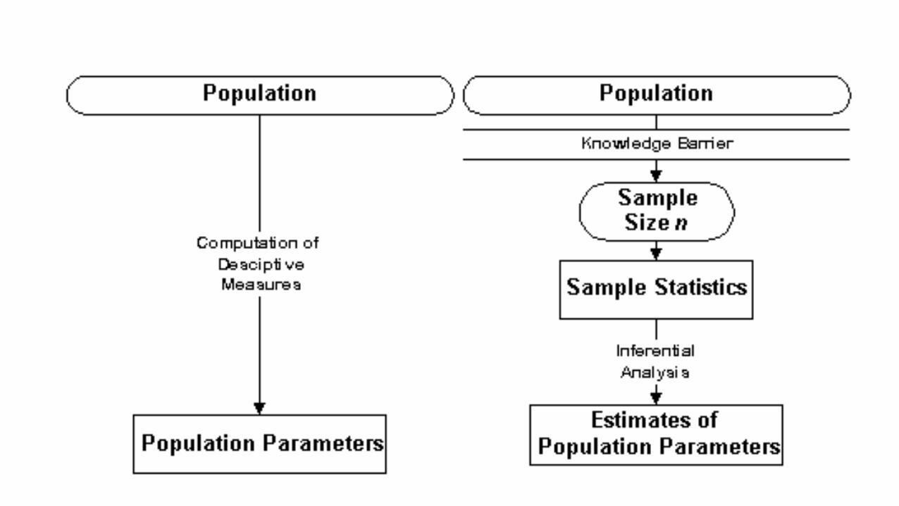
CHAPTER 9 Inference: Estimation  The essential nature of inferential statistics, as verses descriptive statistics is one of knowledge. In descriptive statistics, the analyst has knowledge of the population data. The use of descriptive statistics such as mean, mode, and standard deviation is typically intended for "collapsing" the population data for convenience of reporting or interpretation. In inferential statistics, knowledge about the population is limited to what can be derived from samples. For whatever reason (both economic and logical reasons) it is not possible to view all of the population data, so we must examine our sample data, and make inferences about the population. We can view this process as illustrated in the following figure:

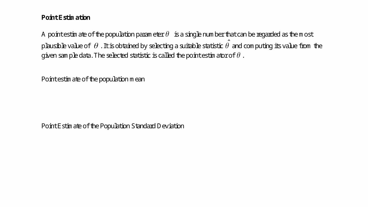
Point Estimation A point estimate of the population parameter is a single number that can be regarded as the most

plausible value of . It is obtained by selecting a suitable statistic ̂ and computing its value from the given sample data. The selected statistic is called the point estimator of . Point estimate of the population mean Point Estimate of the Population Standard Deviation

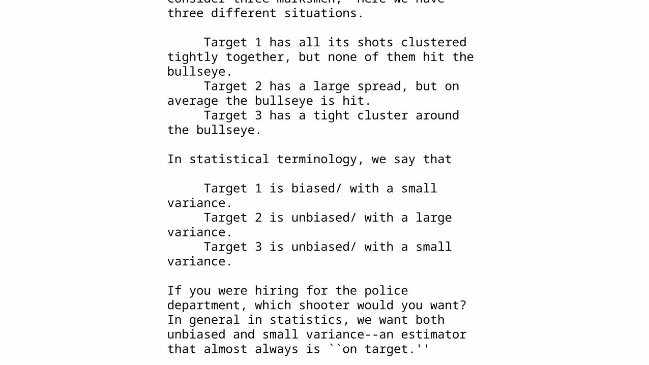
Properties of Point Estimators Consider three marksmen, Here we have three different situations.   Target 1 has all its shots clustered tightly together, but none of them hit the bullseye. Target 2 has a large spread, but on average the bullseye is hit. Target 3 has a tight cluster around the bullseye.  In statistical terminology, we say that   Target 1 is biased/ with a small variance. Target 2 is unbiased/ with a large variance. Target 3 is unbiased/ with a small variance.  If you were hiring for the police department, which shooter would you want? In general in statistics, we want both unbiased and small variance--an estimator that almost always is ``on target.''          

Interval Estimation  Confidence-interval estimate for a population parameter is a set of numbers obtained from the point estimate the parameter, coupled with a "percentage" or probability which characterizes how confident that we are that the parameter lies within the interval.   confidence level is the value of that "percentage" of confidence.  If we wish to be 95% confident that an randomly selected value drawn from a normal distribution, with a mean of 0 and a standard deviation of 1 will be within an interval which is constructed, this interval must be constructed with end-points -z and z such that:   Pr( -z < Z < z) = 0.95  To accomplish the desired results, we must find the appropriate z values for the interval, i.e., this interval would look like the following:   Pr( -1.96 < z < 1.96) = 0.95

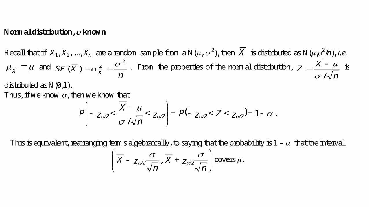
Normal distribution, known Recall that if X1, X2, ..., Xn are a random sample from a N(, 2), then X is distributed as N(,2/n), i.e.,

X and n

XSE X

22)( . From the properties of the normal distribution,

n XZ

/

is

distributed as N(0,1). Thus, if we know , then we know that

= z < Z< zP = z <

n X < zP /2/2/2/2 1

/.

This is equivalent, rearranging terms algebraically, to saying that the probability is 1 – that the interval

nz + X ,

nz X /2/2

covers .

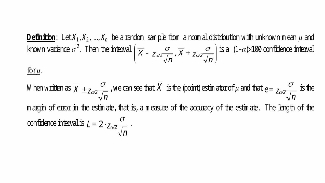
Definition: Let X1, X2, ..., Xn be a random sample from a normal distribution with unknown mean and known variance 2. Then the interval

nz + X ,

nz X /2/2

is a (1–)100confidence interval

for .

When written as n

z X /2

, we can see that X is the (point) estimator of and that n

z = e /2

is the

margin of error in the estimate, that is, a measure of the accuracy of the estimate. The length of the

confidence interval is n

z = L /2

2 .

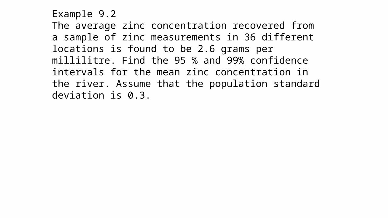
Example 9.2The average zinc concentration recovered from a sample of zinc measurements in 36 different locations is found to be 2.6 grams per millilitre. Find the 95 % and 99% confidence intervals for the mean zinc concentration in the river. Assume that the population standard deviation is 0.3.             

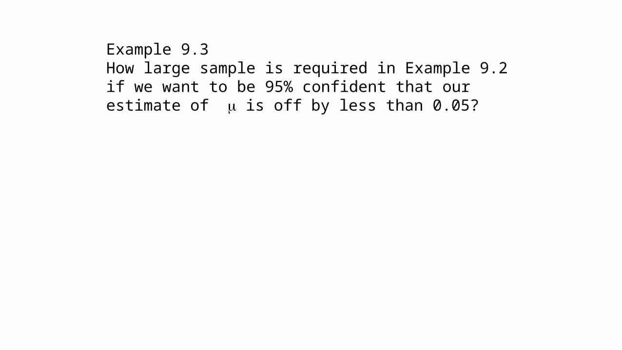
Example 9.3How large sample is required in Example 9.2 if we want to be 95% confident that our estimate of is off by less than 0.05?      

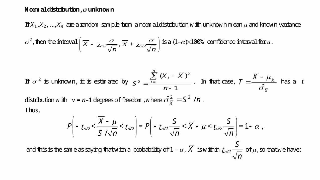
Normal distribution, unknown If X1, X2, ..., Xn are a random sample from a normal distribution with unknown mean and known variance 2, then the interval

nz + X ,

nz X /2/2

is a (1–)100%confidence interval for .

If 2 is unknown, it is estimated by 1

)(1

2

2

n

XXS

n

ii

. In that case, X

XXT

ˆ

has a t

distribution with = n–1 degrees of freedom, where nSX /ˆ 22 . Thus,

= n

St < X <

nS tP = t <

nS X

< tP /2/2/2/2

1

/,

and this is the same as saying that with a probability of 1 – , X is within n

St /2 of , so that we have:

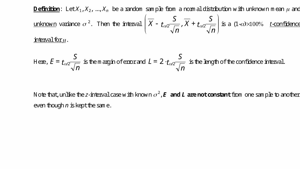
Definition: Let X1, X2, ..., Xn be a random sample from a normal distribution with unknown mean and

unknown variance 2. Then the interval

nS

t + X ,n

St X /2/2 is a (1-t-confidence

interval for .

Here, n

St = E /2 is the margin of error and

nS

t = L /22 is the length of the confidence interval.

Note that, unlike the z-interval case with known 2, E and L are not constant from one sample to another,

even though n is kept the same.

Example 9.4 The contents of 7 similar containers of sulphuric acid are 9.8, 10.2, 10.4, 9.8, 10.0, 10.2, and 9,6 liters. Find 95% confidence interval for the mean of all such containers, assuming an approximate normal distribution.

Large-sample confidence intervals

In constructing a CI for a parameter , we often can find an estimator ̂ which has the following property:

(Note that ̂ is a function of the sample X1, X2, ..., Xn .)

For n large, ̂ is approximately normally distributed with mean and variance 2̂ . Then in such a case

we can say that for n large,

z < < zP /2/2

1

ˆ

ˆ.

This, then, can be the basis of a CI with a coverage probability of approximately 1 – and of the form:

Estimator z /2 (SE), that is, ˆ

ˆ z /2

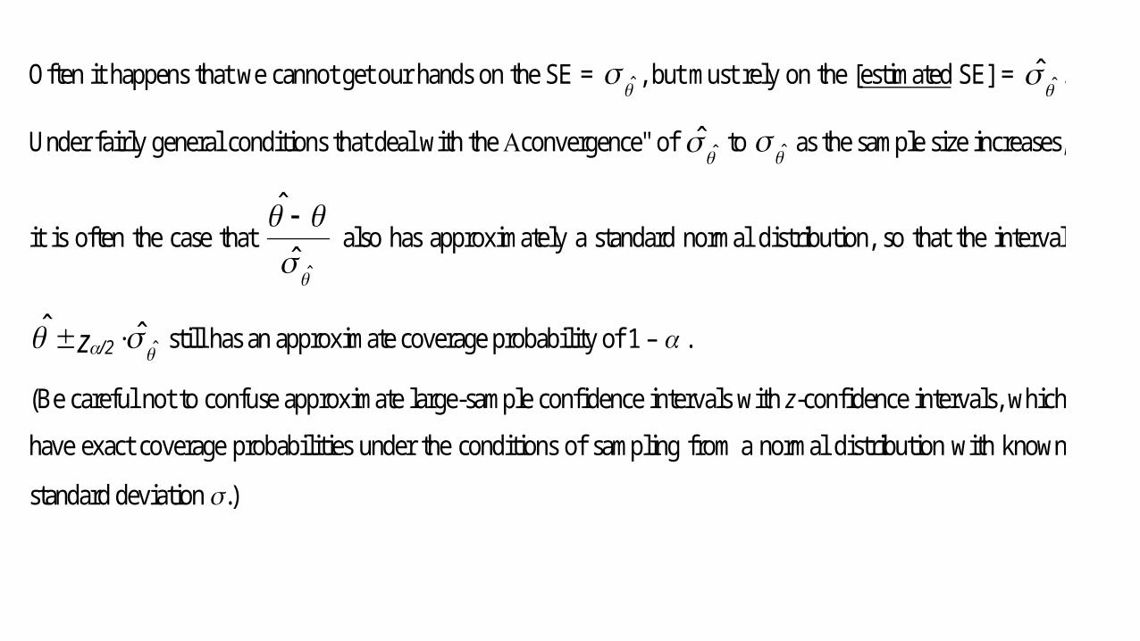
Often it happens that we cannot get our hands on the SE = ˆ , but must rely on the [estimated SE] =

ˆˆ .

Under fairly general conditions that deal with the convergence" of ˆˆ to

ˆ as the sample size increases,

it is often the case that

ˆˆ

ˆ also has approximately a standard normal distribution, so that the interval

ˆˆˆ z /2 still has an approximate coverage probability of 1 – .

(Be careful not to confuse approximate large-sample confidence intervals with z-confidence intervals, which

have exact coverage probabilities under the conditions of sampling from a normal distribution with known

standard deviation .)

9.7. Two samples If we have two populations with means and standard deviations 1 , 1 , and 2 , 2 respectively, the point estimator of the difference between 1 and 2 is given by the statistic 1X - 2X . Therefore to obtain a point estimator of 1- 2 we shall select two independent random samples, one from each population, of size n1 and n2 , and compute the difference 1X - 2X , of the sample means. We must consider the sampling

distribution of 1X - 2X

1X - 2X is approximately normally distributed with mean and variance given by

2121 XX and

2

22

1

212

21 nnXX

Hence

)/()/(

)()(

22

2112

1

2121

nn

XXZ

is approximately a standard normal variable.

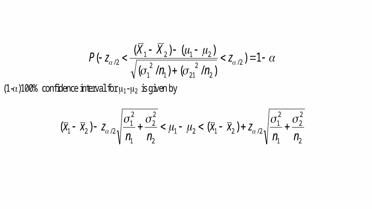
1)

)/()/(

)()(( 2/

22

2112

1

21212/ z

nn

XXzP

(1-)100% confidence interval for 1- 2 is given by

2

22

1

21

2/21212

22

1

21

2/21 )()(nn

zxxnn

zxx

Example 9.6 Two types of engines, A and B, are compared. Gas mileage was measured. 50 experiments were conducted using engine type A and 75 experiments were done for engine type B. The gasoline used and another conditions were held constant. The average gas mileage for A was 36 miles per gallon and for B 42 miles per gallon. Assume that population standard deviations are 6 and 8 for machines A and B respectively. Find a 96% confidence interval on B- A .

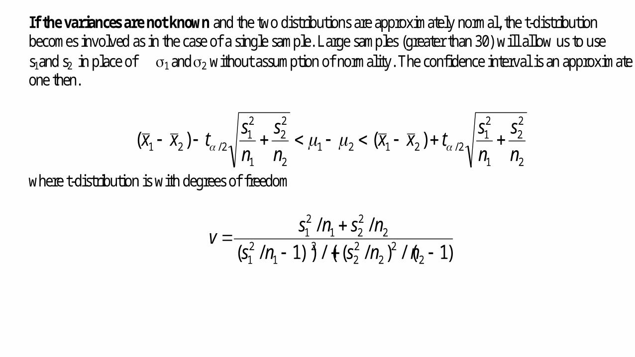
If the variances are not known and the two distributions are approximately normal, the t-distribution becomes involved as in the case of a single sample. Large samples (greater than 30) will allow us to use s1and s2 in place of 1 and 2 without assumption of normality. The confidence interval is an approximate one then.

2

22

1

21

2/21212

22

1

21

2/21 )()(ns

nstxx

ns

nstxx

where t-distribution is with degrees of freedom

)1/()/(/())1/(//

22

222

21

21

2221

21

nnsns

nsnsv

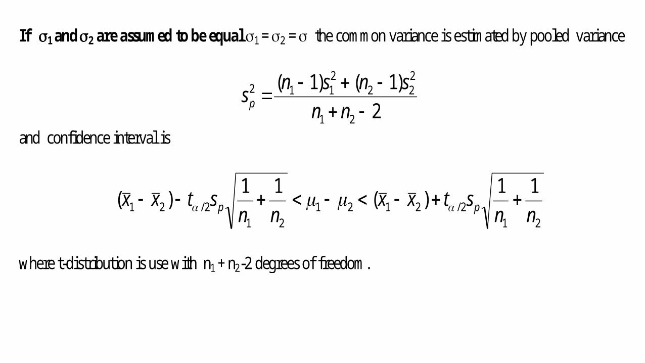
If 1 and 2 are assumed to be equal 1 = 2 = the common variance is estimated by pooled variance

2)1()1(

21

222

2112

nn

snsnsp

and confidence interval is

212/2121

212/21

11)(11)(nn

stxxnn

stxx pp

where t-distribution is use with n1 + n2-2 degrees of freedom.

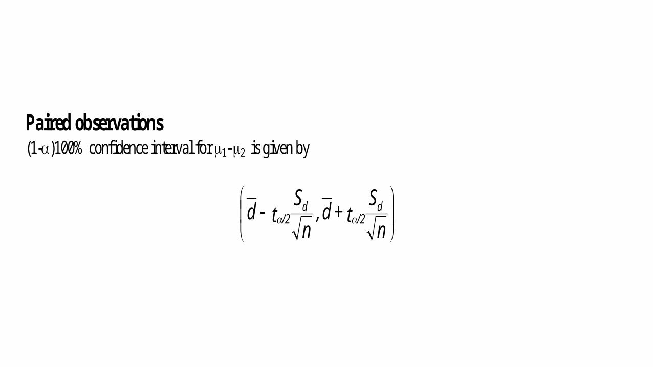
Paired observations (1-)100% confidence interval for 1- 2 is given by

nS

t + d ,n

St d d

/2d

/2

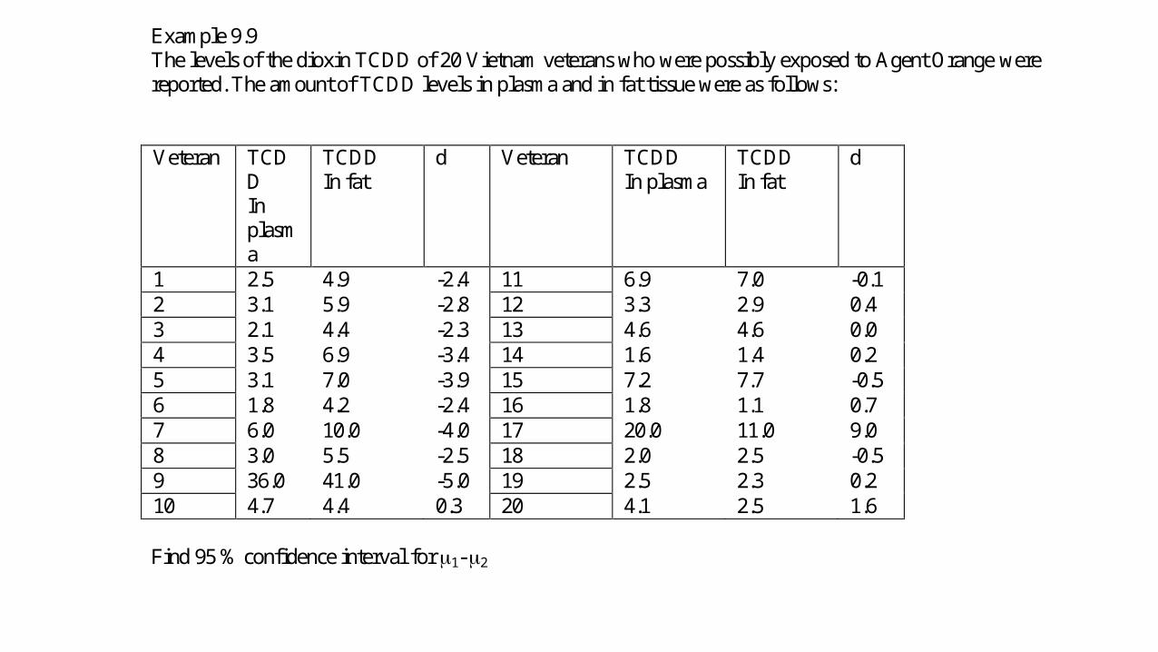
Example 9.9 The levels of the dioxin TCDD of 20 Vietnam veterans who were possibly exposed to Agent Orange were reported. The amount of TCDD levels in plasma and in fat tissue were as follows: Veteran TCD

D In plasma

TCDD In fat

d Veteran TCDD In plasma

TCDD In fat

d

1 2.5 4.9 -2.4 11 6.9 7.0 -0.1 2 3.1 5.9 -2.8 12 3.3 2.9 0.4 3 2.1 4.4 -2.3 13 4.6 4.6 0.0 4 3.5 6.9 -3.4 14 1.6 1.4 0.2 5 3.1 7.0 -3.9 15 7.2 7.7 -0.5 6 1.8 4.2 -2.4 16 1.8 1.1 0.7 7 6.0 10.0 -4.0 17 20.0 11.0 9.0 8 3.0 5.5 -2.5 18 2.0 2.5 -0.5 9 36.0 41.0 -5.0 19 2.5 2.3 0.2 10 4.7 4.4 0.3 20 4.1 2.5 1.6 Find 95 % confidence interval for 1- 2

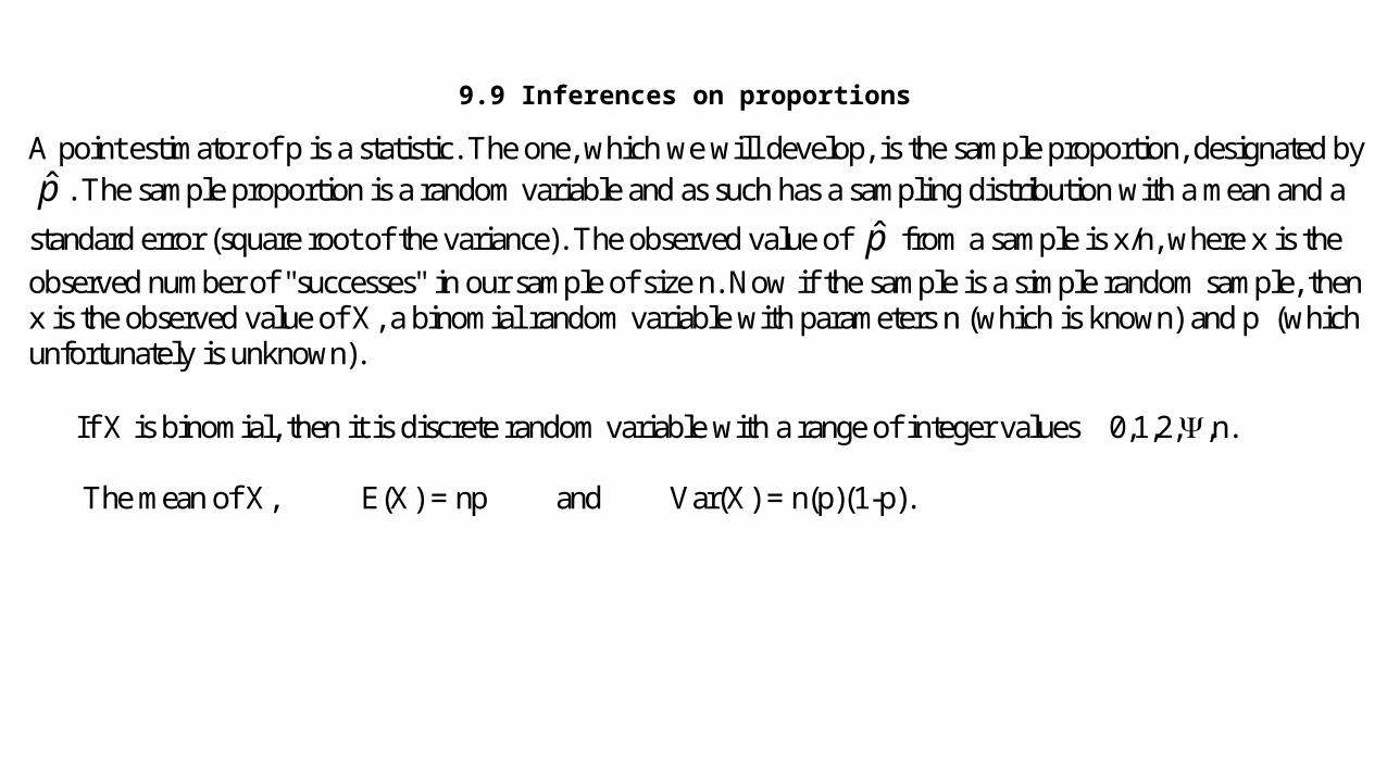
9.9 Inferences on proportions

A point estimator of p is a statistic. The one, which we will develop, is the sample proportion, designated byp̂ . The sample proportion is a random variable and as such has a sampling distribution with a mean and a

standard error (square root of the variance). The observed value of p̂ from a sample is x/n, where x is the observed number of "successes" in our sample of size n. Now if the sample is a simple random sample, then x is the observed value of X, a binomial random variable with parameters n (which is known) and p (which unfortunately is unknown). If X is binomial, then it is discrete random variable with a range of integer values 0,1,2,,n. The mean of X, E(X) = np and Var(X) = n(p)(1-p).

Since p̂ = X/n, p̂ is also a discrete random variable that takes on the (n + 1) possible values of

0,1/n,2/n,,1. The expected value of p̂ ,

E( p̂ ) = E(X)/n = n(p)/n = p. This says that p̂ is an unbiased estimator of p .

The variance of p̂ ,

Var( p̂ ) = Var(X)/n2 =p (1 -p )/n.

This says that p̂ is also a consistent estimator of p.

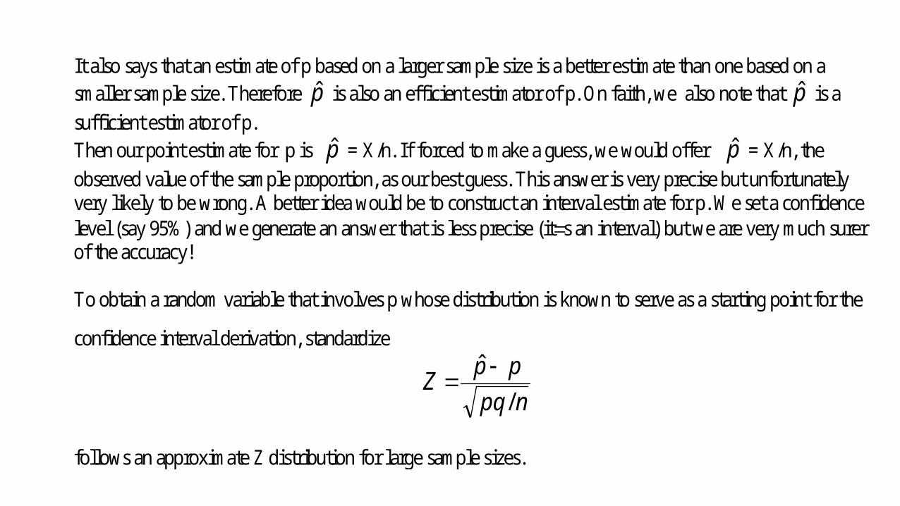
It also says that an estimate of p based on a larger sample size is a better estimate than one based on a smaller sample size. Therefore p̂ is also an efficient estimator of p. On faith, we also note that p̂ is a sufficient estimator of p. Then our point estimate for p is p̂ = X/n. If forced to make a guess, we would offer p̂ = X/n, the observed value of the sample proportion, as our best guess. This answer is very precise but unfortunately very likely to be wrong. A better idea would be to construct an interval estimate for p. We set a confidence level (say 95%) and we generate an answer that is less precise (its an interval) but we are very much surer of the accuracy! To obtain a random variable that involves p whose distribution is known to serve as a starting point for the

confidence interval derivation, standardize

npqppZ/

ˆ

follows an approximate Z distribution for large sample sizes.

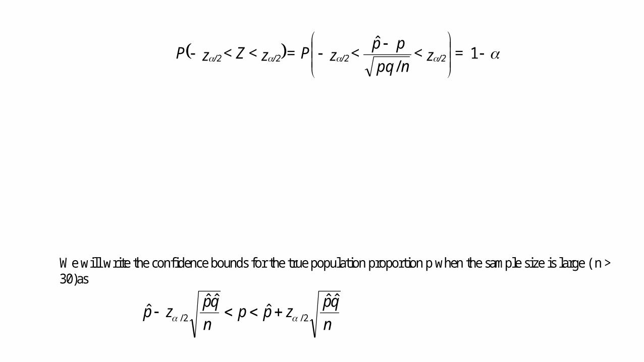
= z <

npqp p < zP= z < Z< zP /2/2/2/2 1/

ˆ

We will write the confidence bounds for the true population proportion p when the sample size is large ( n > 30)as

nqpzpp

nqpzp

ˆˆˆˆˆˆ 2/2/

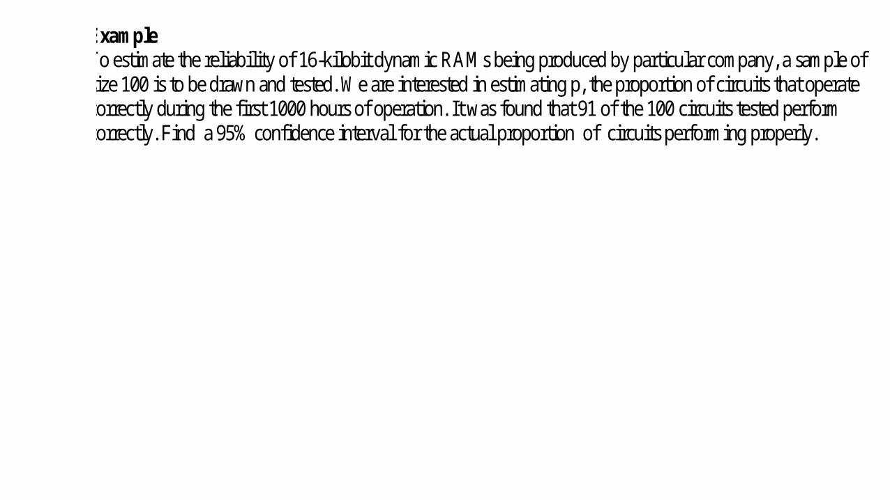
Example To estimate the reliability of 16-kilobit dynamic RAMs being produced by particular company, a sample of size 100 is to be drawn and tested. We are interested in estimating p, the proportion of circuits that operate correctly during the first 1000 hours of operation. It was found that 91 of the 100 circuits tested perform correctly. Find a 95% confidence interval for the actual proportion of circuits performing properly.

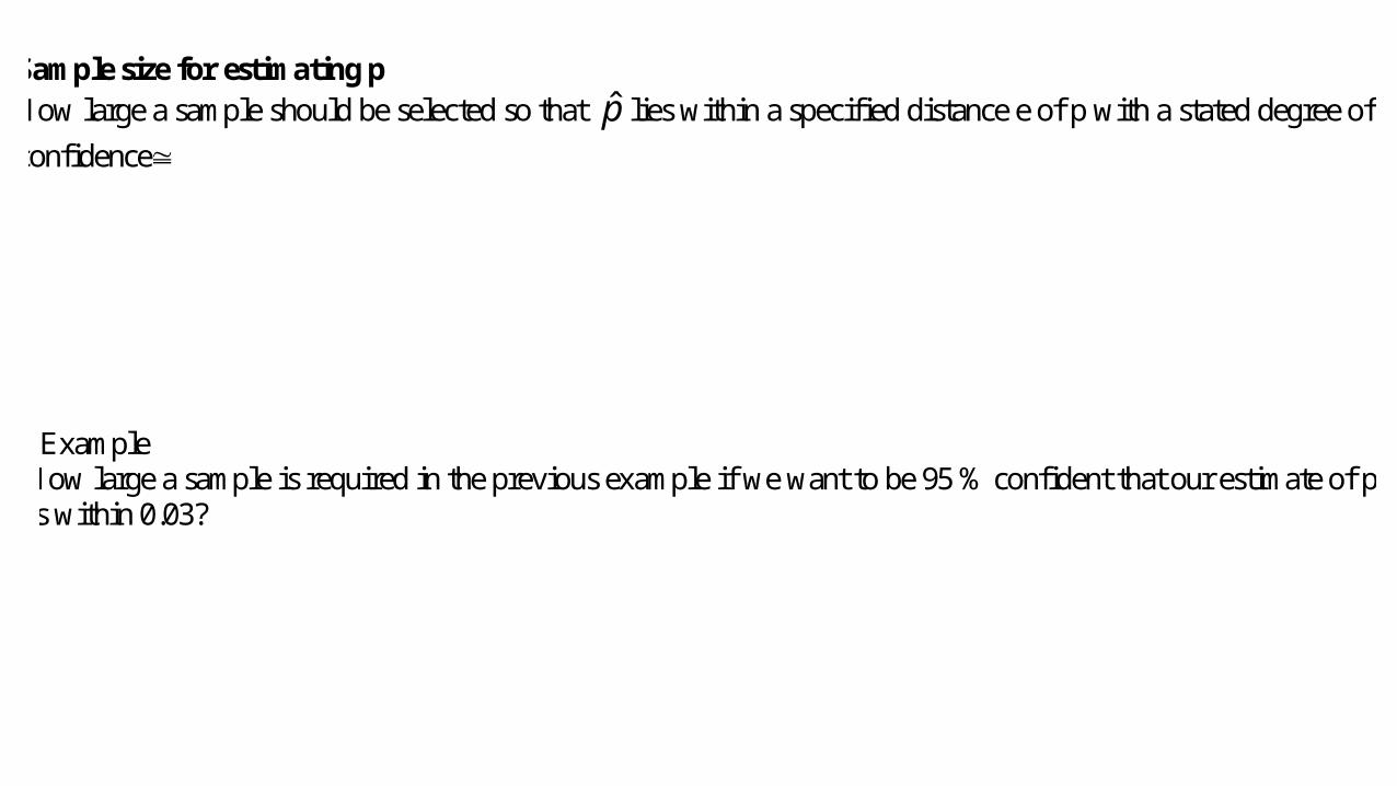
Sample size for estimating p How large a sample should be selected so that p̂ lies within a specified distance e of p with a stated degree of confidence

Example How large a sample is required in the previous example if we want to be 95 % confident that our estimate of p is within 0.03?

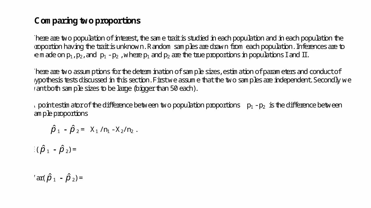
Comparing two proportions There are two population of interest, the same trait is studied in each population and in each population the proportion having the trait is unknown. Random samples are drawn from each population. Inferences are to be made on p1, p2, and p1 - p2 , where p1 and p2 are the true proportions in populations I and II. There are two assumptions for the determination of sample sizes, estimation of parameters and conduct of hypothesis tests discussed in this section. First we assume that the two samples are independent. Secondly we want both sample sizes to be large (bigger than 50 each). A point estimator of the difference between two population proportions p1 - p2 is the difference between sample proportions

p̂ 1 - p̂ 2 = X1 / n1 - X2/ n2 . E( p̂ 1 - p̂ 2) = Var( p̂ 1 - p̂ 2) =

The statistic p̂ 1 - p̂ 2 is an unbiased estimator for p1 - p2 To obtain a random variable that involves p1 - p2 whose distribution is known , at least approximately to serve as a starting point for the confidence interval derivation, standardize

)/()/(

)()ˆˆ(

222111

2121

nqpnqp

ppppZ

Applying the notion of constructing confidence intervals the proposed bounds for a confidence interval on p1 - p2 will be

2

22

1

112/2121

2

22

1

112/21

ˆˆˆˆ)ˆˆ(

ˆˆˆˆ)ˆˆ(

nqp

nqpzpppp

nqp

nqpzpp

Example 9.13: A certain change in a process for manufacture of component parts is being considered. Samples are taken using both the existing and the new procedure so as to determine if the new process results in an improvement. If 75 of 1500 items from the existing procedure were found to be defective and 80 of 2000 items from the new procedure were found to be defective, find a 90 % confidence interval for the true difference in the fraction of defectives between the existing and the new process.

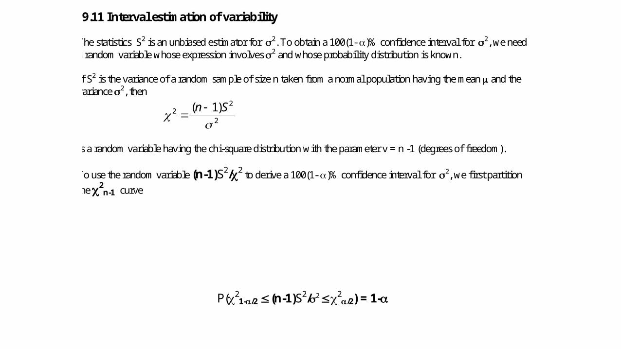
9.11 Interval estimation of variability The statistics S2 is an unbiased estimator for 2. To obtain a 100(1- )% confidence interval for 2, we need a random variable whose expression involves 2 and whose probability distribution is known. If S2 is the variance of a random sample of size n taken from a normal population having the mean and the variance 2, then

2

22 )1(

Sn

is a random variable having the chi-square distribution with the parameter v = n -1 (degrees of freedom). To use the random variable (n-1)S2/2 to derive a 100(1- )% confidence interval for 2, we first partition the 2

n-1 curve

P(21-/2 (n-1)S2/2 2

/2) = 1-

Theorem Let X1, X2, ..., Xn are a random sample from a normal population with a mean and standard deviation . The lower and upper bounds, L1 and L2 respectively, for a 100(1- )% confidence interval for 2, are given by L1 = (n-1)S2/2

/2 ) and L2 = (n-1)S2/21-/2 .

Example. 25 observations on the relative I/O content for a large consulting firm over randomly selected one-hour period are obtained. s2 = 1.407 s = 1.186. Construct a 95% confidence interval on the standard deviation of the relative I/O content for this instalation.

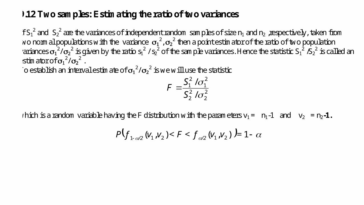
9.12 Two samples: Estimating the ratio of two variances If S1

2 and S22 are the variances of independent random samples of size n1 and n2 ,respectively, taken from

two normal populations with the variance 2,2 then a point estimator of the ratio of two population variances 2/2 is given by the ratio s1

2 / s22 of the sample variances. Hence the statistic S1

2 /S22 is called an

estimator of 2/2 . To establish an interval estimate of 2/2 is we will use the statistic

22

22

21

21

//

SSF

which is a random variable having the F distribution with the parameters v1 = n1-1 and v2 = n2-1.

= vvf < F < vvfP /2/2 1),(),( 21211

Exercise 9 p.275 Construct a 98% confidence interval for , where are , respectively, the standard deviations for the distance obtained per litre of fuel by the Volkswagen and Toyota minitrucks.

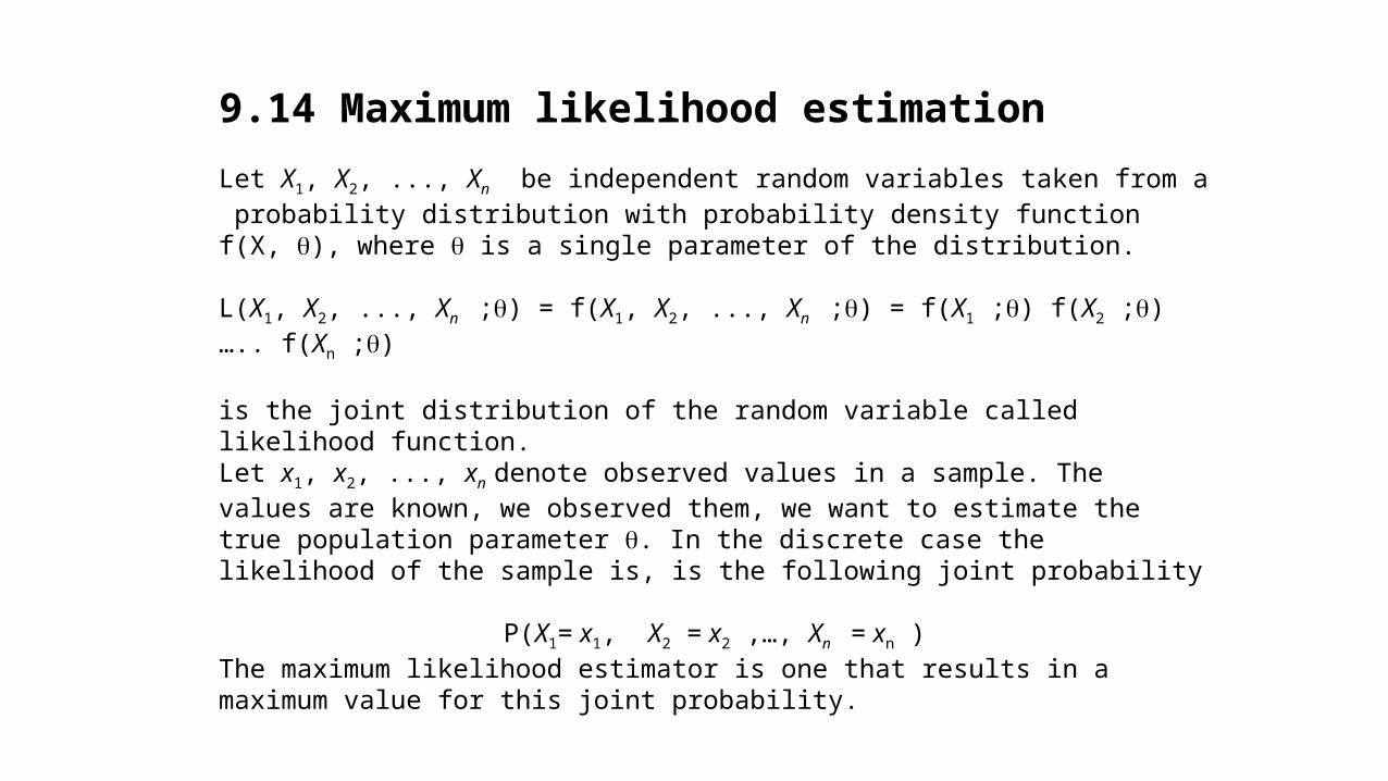
9.14 Maximum likelihood estimation Let X1, X2, ..., Xn be independent random variables taken from a probability distribution with probability density function f(X, ), where is a single parameter of the distribution.  L(X1, X2, ..., Xn ;) = f(X1, X2, ..., Xn ;) = f(X1 ;) f(X2 ;)….. f(Xn ;) is the joint distribution of the random variable called likelihood function. Let x1, x2, ..., xn denote observed values in a sample. The values are known, we observed them, we want to estimate the true population parameter . In the discrete case the likelihood of the sample is, is the following joint probability 

P(X1= x1, X2 = x2 ,…, Xn = xn )The maximum likelihood estimator is one that results in a maximum value for this joint probability.

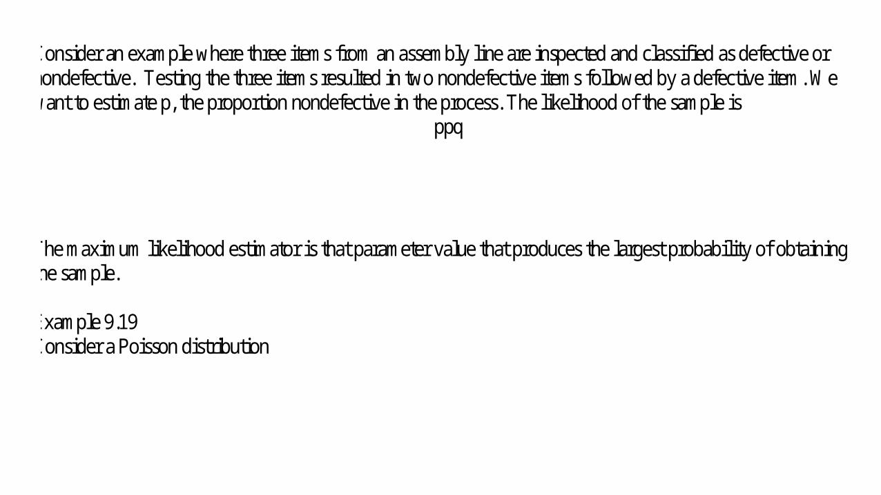
Consider an example where three items from an assembly line are inspected and classified as defective or nondefective. Testing the three items resulted in two nondefective items followed by a defective item. We want to estimate p, the proportion nondefective in the process. The likelihood of the sample is

ppq The maximum likelihood estimator is that parameter value that produces the largest probability of obtaining the sample. Example 9.19 Consider a Poisson distribution

Example 9.21 Suppose 15 rats are used in a biomedical study where the rats are injected with cancer cells and given a cancer drug that is designed to increase their survival rate. 14, 17, 27, 18, 12, 8, 22, 13, 19, 12 Assume that the exponential distribution applies.