Chapter 9

Fourier Transforms and plotting softwares

After studying the present chapter, you will be able to

i) Compute Fourier transforms of functions using the Scilab software ii) Use the PlotDigitizer software in Linux to digitize continuous functions from any

source that is available as a jpeg file iii) Use GNU plot softare in Linux to plot 3D plots iv) Use Xmgrace software for graphics.

9.1 Introduction

In this chapter, we consider the application of the scilab software for calculating Fourier transforms. A few more useful softwares such as the PlotDigitizer, the GNU plot softare in Linux to plot 3D plots and the Xmgrace software will also be introduced. Fourier transforms (FTs) and Laplace transforms (the later is left as an exercise) are extensively used in engineering and science and in chemistry as well. The FTs in particular are so important, that many instruments such as FT NMRs and FT IRs include these transforms as a part of the equipment software. Thus, a chemistry student will certainly benefit by knowing how these things are done and these are not really too complex in principle. First we consider the FTs.

9.2 Fourier Transforms

We will not discuss in much detail the theoretical background of the Fourier series or Fourier transforms as our task in only computational. We will define the transforms and illustrate how to use the scilab software to get one of these transforms and let you do the remaining as exercises. The main weapon to check the accuracy of your result is that when you do the inverse transform, you should recover the original function. For example, if you invert a matrix A anc call the inverse Ainv, the inverse of Ainv should be A itself, within a predefined accuracy. A simple way to think of visualizing how to do the integrals is to digitize the integrand over a wide enough range and sum it and multiply it with the increment in the x direction, ie. dx for a one dimensional integral.

The cosine, sine and the Fourier transform pairs are defined as follows:

Cosine transform pair

dxkxxfkFc )(cos)()/2()(0∫∞

= π and dkkxkFxf c )(cos)()/2()(0∫∞

= π (9.1)

Sine transform pair

dxkxxfkFs )(sin)()/2()(0∫∞

= π and dkkxkFxf s )(sin)()/2()(0∫∞

= π (9.2)

Fourier transform pair

dxxkixfkF )(exp)()2/1()( −= ∫∞

∞−

π and dxxkixFxf )(exp)()2/1()( ∫∞

∞−

= π (9.3)

In books and literature, you will find different versions of these transforms, with signs in the exponent different and factors of 2π also used in alternative ways. However, all these are equivalent and you should compare carefully and match your results with those of other books. The function when f is transformed, it denoted by F, ie, its transform is represented as F. For cos and sine transforms, there are subscripts c and s. The Fourier transform uses complex variables and the resulting transforms may also be functions of a complex variable. In the following tables, we give examples of these transforms which will be useful when you do test computations on these functions.

Table of cos, sine and Fourier transforms

Transform f(x) F(k) cos exp(-ax), a>0 )/2( π [ ( a / (a2 + k2) ] cos exp(-ax2), a>0 )2/1( a exp(-k2/4a)

sin exp(-x) )/2( π [ ( k / (1 + k2) ] sin x exp(-ax2), a>0 [ 2/3)2/( ak ] exp(-k2/4a)

Fourier 1 / (a2 + x2); a > 0 )2/(π exp(-a| k|)/a Fourier exp(-ax), x>0, (a >

0) 0, otherwise

1/[ )2( π (a + i k)]

Fourier exp(-ax2), a>0 )2/1( a exp(-k2/4a)

Here, |k| is the absolute value of k and i = 1−

To use in scilab, we need to compute the values of the functions in the f(x) column for a large number of points and then call the appropriate function from the function library.

9.2aThe cos Transform (DCT, the discrete cosine transform)

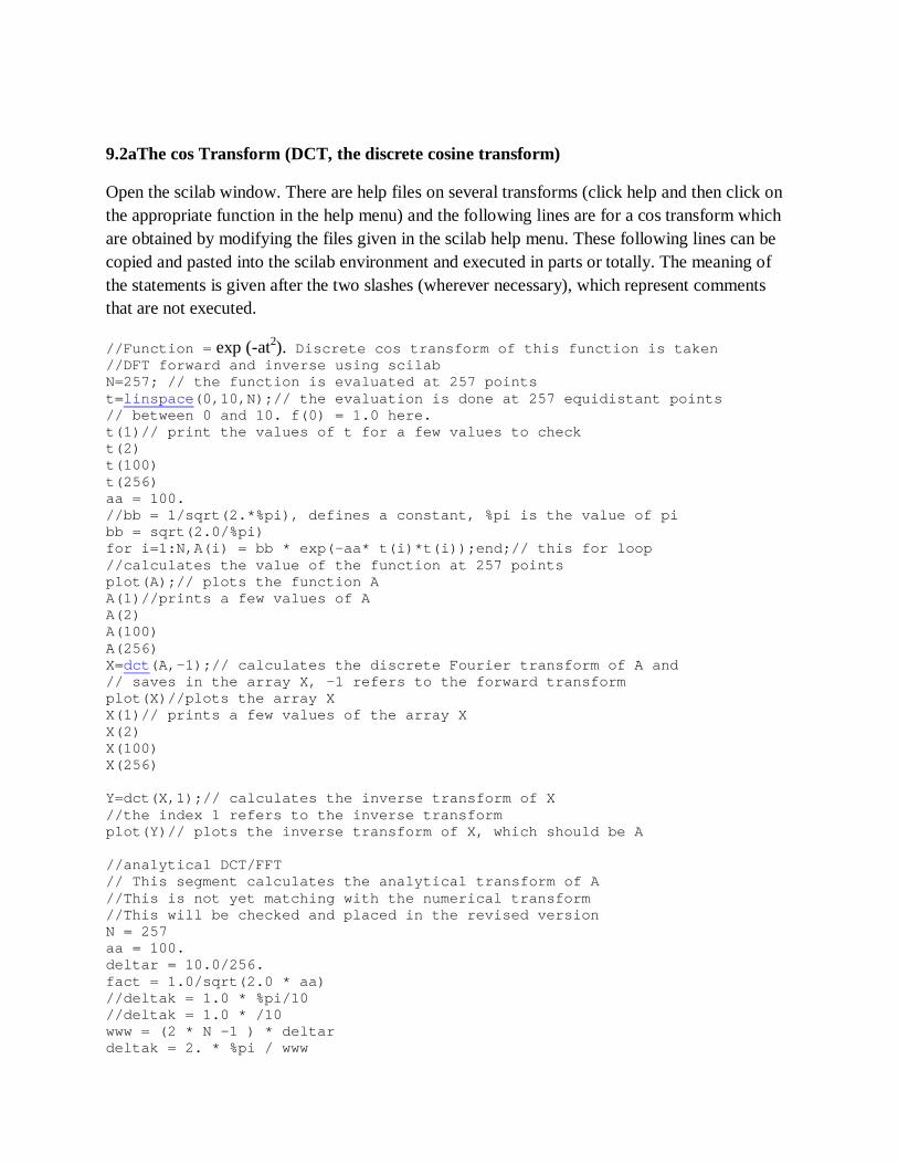
Open the scilab window. There are help files on several transforms (click help and then click on the appropriate function in the help menu) and the following lines are for a cos transform which are obtained by modifying the files given in the scilab help menu. These following lines can be copied and pasted into the scilab environment and executed in parts or totally. The meaning of the statements is given after the two slashes (wherever necessary), which represent comments that are not executed.

//Function = exp (-at2). Discrete cos transform of this function is taken //DFT forward and inverse using scilab N=257; // the function is evaluated at 257 points t=linspace(0,10,N);// the evaluation is done at 257 equidistant points // between 0 and 10. f(0) = 1.0 here. t(1)// print the values of t for a few values to check t(2) t(100) t(256) aa = 100. //bb = 1/sqrt(2.*%pi), defines a constant, %pi is the value of pi bb = sqrt(2.0/%pi) for i=1:N,A(i) = bb * exp(-aa* t(i)*t(i));end;// this for loop //calculates the value of the function at 257 points plot(A);// plots the function A A(1)//prints a few values of A A(2) A(100) A(256) X=dct(A,-1);// calculates the discrete Fourier transform of A and // saves in the array X, -1 refers to the forward transform plot(X)//plots the array X X(1)// prints a few values of the array X X(2) X(100) X(256) Y=dct(X,1);// calculates the inverse transform of X //the index 1 refers to the inverse transform plot(Y)// plots the inverse transform of X, which should be A //analytical DCT/FFT // This segment calculates the analytical transform of A //This is not yet matching with the numerical transform //This will be checked and placed in the revised version N = 257 aa = 100. deltar = 10.0/256. fact = 1.0/sqrt(2.0 * aa) //deltak = 1.0 * %pi/10 //deltak = 1.0 * /10 www = (2 * N -1 ) * deltar deltak = 2. * %pi / www

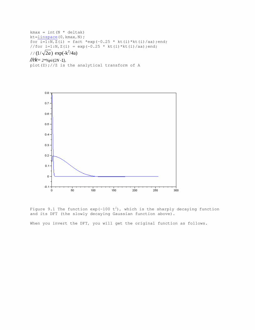
kmax = int(N * deltak) kt=linspace(0,kmax,N); for i=1:N,Z(i) = fact *exp(-0.25 * kt(i)*kt(i)/aa);end; //for i=1:N,Z(i) = exp(-0.25 * kt(i)*kt(i)/aa);end;

// )2/1( a exp(-k2/4a) //rk= 2*%pi/(2N -1), plot(Z);//Z is the analytical transform of A

Figure 9.1 The function exp(-100 t2), which is the sharply decaying function and its DFT (the slowly decaying Gaussian function above). When you invert the DFT, you will get the original function as follows.

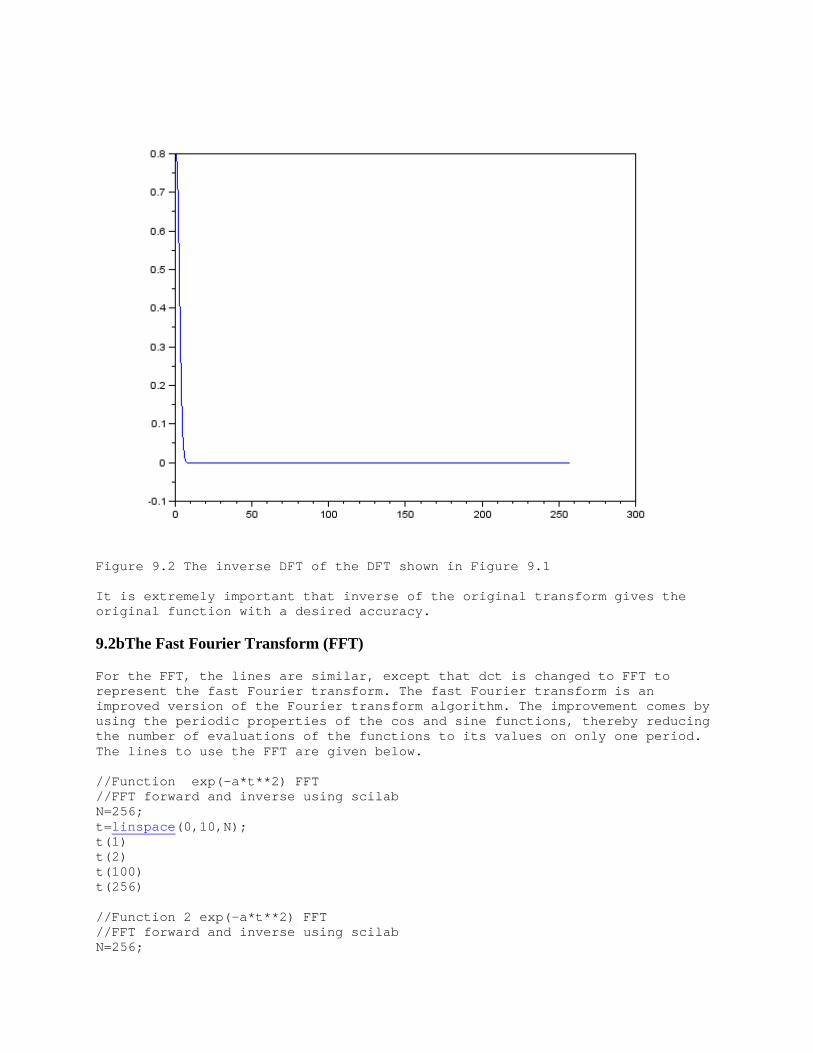
Figure 9.2 The inverse DFT of the DFT shown in Figure 9.1 It is extremely important that inverse of the original transform gives the original function with a desired accuracy. 9.2bThe Fast Fourier Transform (FFT)

For the FFT, the lines are similar, except that dct is changed to FFT to represent the fast Fourier transform. The fast Fourier transform is an improved version of the Fourier transform algorithm. The improvement comes by using the periodic properties of the cos and sine functions, thereby reducing the number of evaluations of the functions to its values on only one period. The lines to use the FFT are given below. //Function exp(-a*t**2) FFT //FFT forward and inverse using scilab N=256; t=linspace(0,10,N); t(1) t(2) t(100) t(256) //Function 2 exp(-a*t**2) FFT //FFT forward and inverse using scilab N=256;

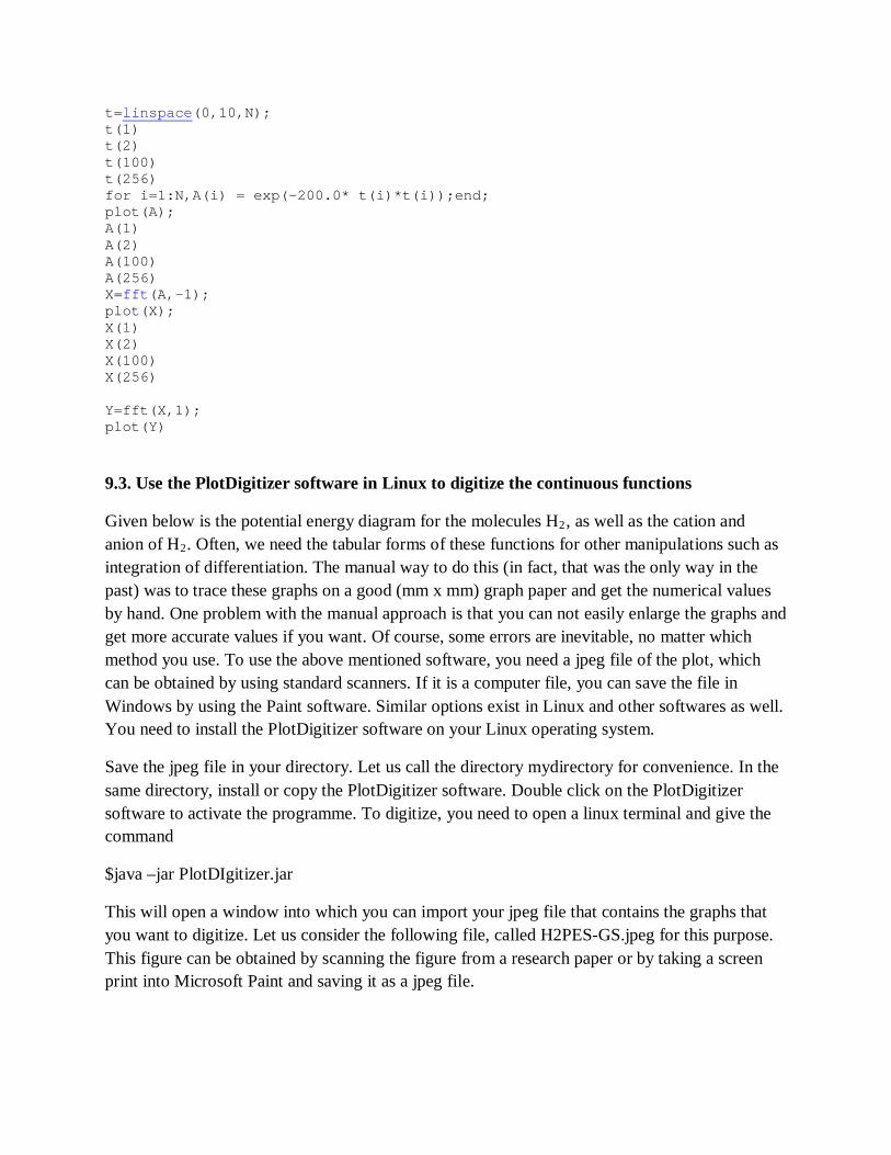
t=linspace(0,10,N); t(1) t(2) t(100) t(256) for i=1:N,A(i) = exp(-200.0* t(i)*t(i));end; plot(A); A(1) A(2) A(100) A(256) X=fft(A,-1); plot(X); X(1) X(2) X(100) X(256) Y=fft(X,1); plot(Y)

9.3. Use the PlotDigitizer software in Linux to digitize the continuous functions

Given below is the potential energy diagram for the molecules H2, as well as the cation and anion of H2. Often, we need the tabular forms of these functions for other manipulations such as integration of differentiation. The manual way to do this (in fact, that was the only way in the past) was to trace these graphs on a good (mm x mm) graph paper and get the numerical values by hand. One problem with the manual approach is that you can not easily enlarge the graphs and get more accurate values if you want. Of course, some errors are inevitable, no matter which method you use. To use the above mentioned software, you need a jpeg file of the plot, which can be obtained by using standard scanners. If it is a computer file, you can save the file in Windows by using the Paint software. Similar options exist in Linux and other softwares as well. You need to install the PlotDigitizer software on your Linux operating system.

Save the jpeg file in your directory. Let us call the directory mydirectory for convenience. In the same directory, install or copy the PlotDigitizer software. Double click on the PlotDigitizer software to activate the programme. To digitize, you need to open a linux terminal and give the command

$java –jar PlotDIgitizer.jar

This will open a window into which you can import your jpeg file that contains the graphs that you want to digitize. Let us consider the following file, called H2PES-GS.jpeg for this purpose. This figure can be obtained by scanning the figure from a research paper or by taking a screen print into Microsoft Paint and saving it as a jpeg file.

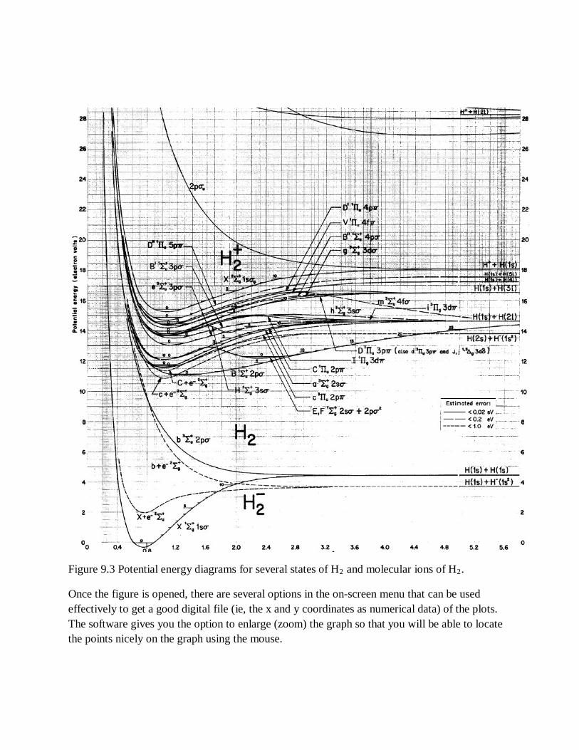
Figure 9.3 Potential energy diagrams for several states of H2 and molecular ions of H2.

Once the figure is opened, there are several options in the on-screen menu that can be used effectively to get a good digital file (ie, the x and y coordinates as numerical data) of the plots. The software gives you the option to enlarge (zoom) the graph so that you will be able to locate the points nicely on the graph using the mouse.

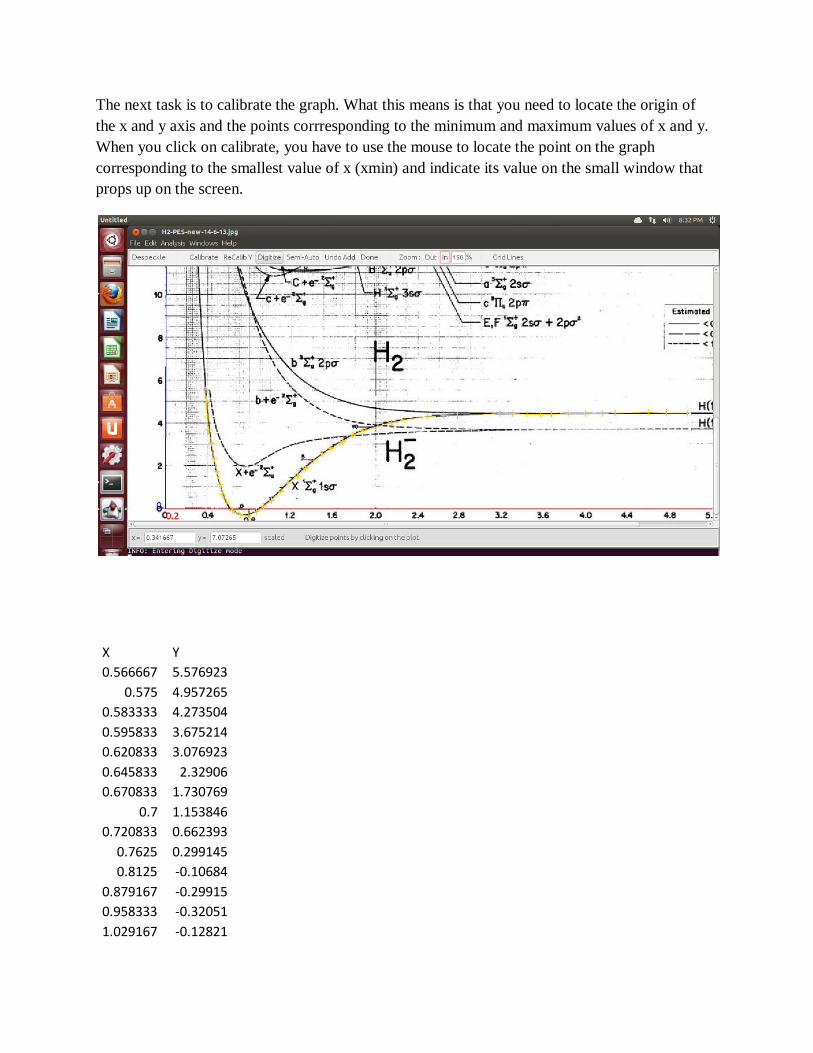
The next task is to calibrate the graph. What this means is that you need to locate the origin of the x and y axis and the points corrresponding to the minimum and maximum values of x and y. When you click on calibrate, you have to use the mouse to locate the point on the graph corresponding to the smallest value of x (xmin) and indicate its value on the small window that props up on the screen.

X Y 0.566667 5.576923

0.575 4.957265 0.583333 4.273504 0.595833 3.675214 0.620833 3.076923 0.645833 2.32906 0.670833 1.730769

0.7 1.153846 0.720833 0.662393

0.7625 0.299145 0.8125 -0.10684

0.879167 -0.29915 0.958333 -0.32051 1.029167 -0.12821

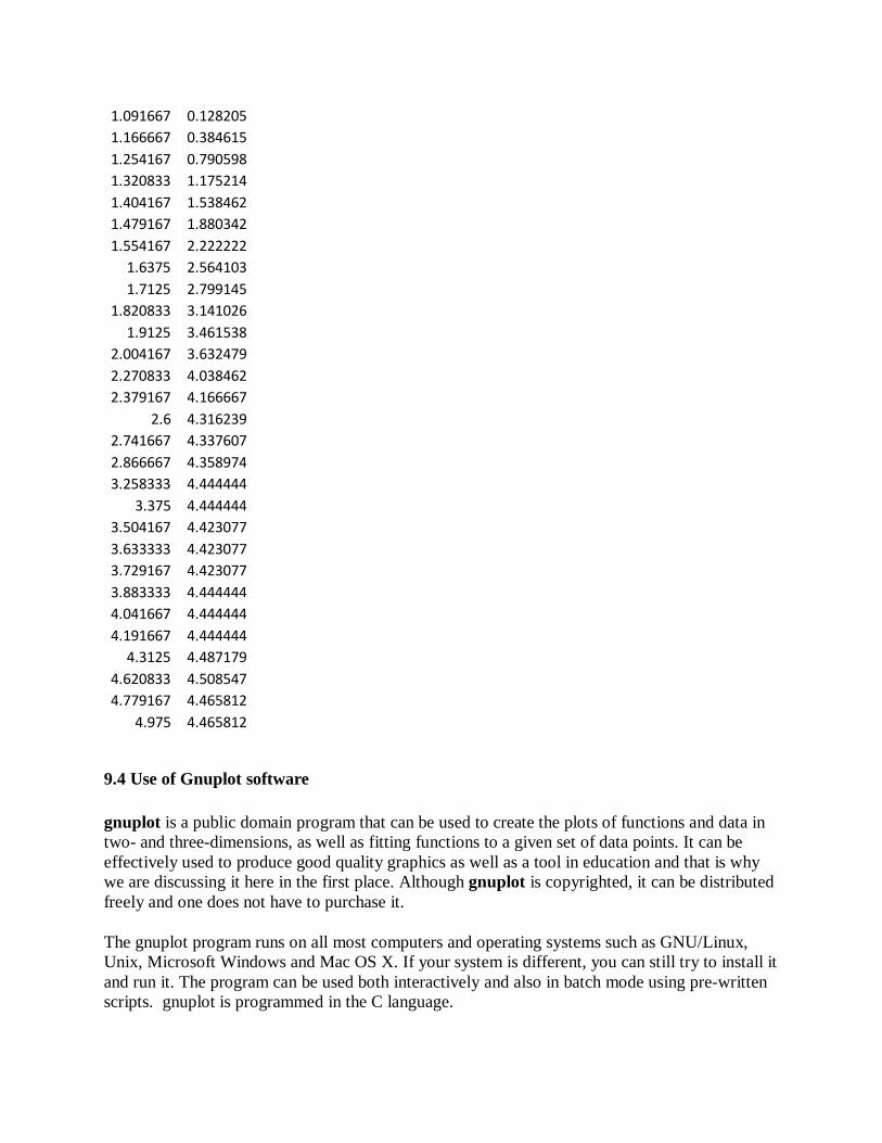
1.091667 0.128205 1.166667 0.384615 1.254167 0.790598 1.320833 1.175214 1.404167 1.538462 1.479167 1.880342 1.554167 2.222222

1.6375 2.564103 1.7125 2.799145

1.820833 3.141026 1.9125 3.461538

2.004167 3.632479 2.270833 4.038462 2.379167 4.166667

2.6 4.316239 2.741667 4.337607 2.866667 4.358974 3.258333 4.444444

3.375 4.444444 3.504167 4.423077 3.633333 4.423077 3.729167 4.423077 3.883333 4.444444 4.041667 4.444444 4.191667 4.444444

4.3125 4.487179 4.620833 4.508547 4.779167 4.465812

4.975 4.465812

9.4 Use of Gnuplot software

gnuplot is a public domain program that can be used to create the plots of functions and data in two- and three-dimensions, as well as fitting functions to a given set of data points. It can be effectively used to produce good quality graphics as well as a tool in education and that is why we are discussing it here in the first place. Although gnuplot is copyrighted, it can be distributed freely and one does not have to purchase it.

The gnuplot program runs on all most computers and operating systems such as GNU/Linux, Unix, Microsoft Windows and Mac OS X. If your system is different, you can still try to install it and run it. The program can be used both interactively and also in batch mode using pre-written scripts. gnuplot is programmed in the C language.

Some of the things that you can do with gnuplot are

• Plotting two-dimensional functions and data points in many different styles (points, lines, error bars)

• Plotting three-dimensional data points and surfaces in many different styles (contour plot, mesh)

• Algebraic computation in integer, float and complex arithmetic

The results of the graphics can be saved in different file formats and output devices. Extensive help on gnuplot is available on the Internet and this section is also written by adapting the available literature on internet and using it for the purpose of chemical computations.

As in the case of any other software, there are commands specific to gnuplot. The following lines, which are self explanatory, are the instructions to plot the curve that is shown below. Before typing these lines, you need to invoke gnuplot by typing gnuplot at the command prompt, $ in linux.

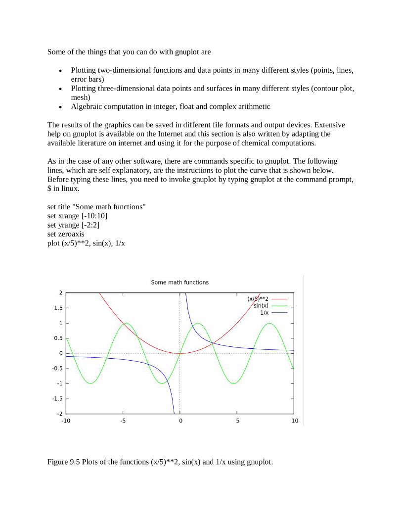
set title "Some math functions" set xrange [-10:10] set yrange [-2:2] set zeroaxis plot (x/5)**2, sin(x), 1/x

Figure 9.5 Plots of the functions (x/5)**2, sin(x) and 1/x using gnuplot.

The explanation of the functions is now included in parentheses { }. set title "Some math functions" {gives the title to the graph} set xrange [-10:10] {gives the range to the x axis. You can alter the range as per your need} set yrange [-2:2] {gives the range to the y axis} set zeroaxis { sets or draws the zero axis line. You may try plotting withour this line} plot (x/4)**2, sin(x), 1/x {This plots the graphs of the three functions indicates}

Gnuplot is freeware authored by a collection of volunteers, who do not make any legal statement about the functioning and the compliance or non-compliance of gnuplot or its uses. There is also no warranty whatsoever. Although this is to be used at the user’s risk, its utility is impressive.

For additional information, see the main gnuplot web page http://www.gnuplot.info. Some documentation and tutorials are available in other languages than English. See the section "Localized learning pages about gnuplot", for the most up-to-date list in the web-site http://gnuplot.sourceforge.net/help.html.

9.4a Fitting Functions using gnuplot

Suppose we have (x,y) data of some function and we want to fit a good function through these data points. Let the data be saved in a file named ‘ref.dat’. To plot this (x,y) data, we can simply type in gnuplot, plot ‘ref.dat’ and the graph will appear in a new window.

To fit this data, we need to have a functional form in mind. In our case, the (x,y) in question is a potential energy function which needs to be fitted into a Morse potential energy curve.

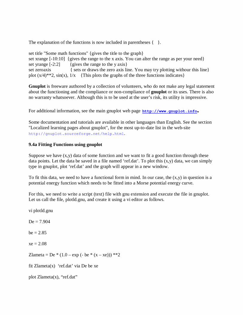
For this, we need to write a script (text) file with gnu extension and execute the file in gnuplot. Let us call the file, plotld.gnu, and create it using a vi editor as follows.

vi plotld.gnu

De = 7.904

be = 2.85

xe = 2.08

Zlameta = De * (1.0 – exp (- be * (x – xe))) **2

fit Zlameta(x) ‘ref.dat’ via De be xe

plot Zlameta(x), “ref.dat”

In gnuplot, you execute this file by typing

gnuplot> load “./plotld.gnu”

gnuplot> plot “ref.dat”

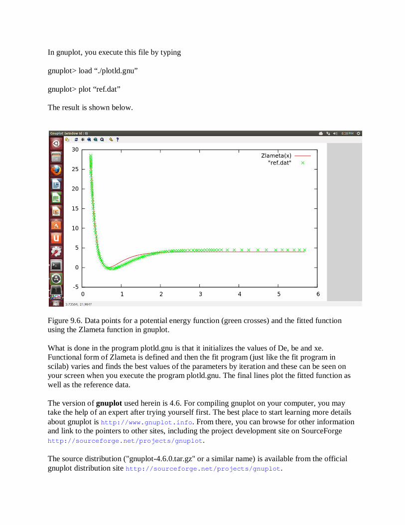
The result is shown below.

Figure 9.6. Data points for a potential energy function (green crosses) and the fitted function using the Zlameta function in gnuplot.

What is done in the program plotld.gnu is that it initializes the values of De, be and xe. Functional form of Zlameta is defined and then the fit program (just like the fit program in scilab) varies and finds the best values of the parameters by iteration and these can be seen on your screen when you execute the program plotld.gnu. The final lines plot the fitted function as well as the reference data.

The version of gnuplot used herein is 4.6. For compiling gnuplot on your computer, you may take the help of an expert after trying yourself first. The best place to start learning more details about gnuplot is http://www.gnuplot.info. From there, you can browse for other information and link to the pointers to other sites, including the project development site on SourceForge http://sourceforge.net/projects/gnuplot.

The source distribution ("gnuplot-4.6.0.tar.gz" or a similar name) is available from the official gnuplot distribution site http://sourceforge.net/projects/gnuplot.

The documentation is included in the source distribution. In the docs subdirectory, there are files that include the following details

• a PDF version of the user manual • a Unix man page, which says how to start gnuplot , and • a tutorial on using gnuplot with LATEX

Online gnuplot documentation is also available at http://gnuplot.sourceforge.net/documentation.html.

There is a directory of worked examples in the source distribution. These examples, and the resulting plots, may also be found at http://gnuplot.sourceforge.net/demo/. There are several worked out examples. We are listing a couple of important uses.

9.4bThree dimensional plots using gnuplot

The following lines illustrate plotting a 3D plot. You have to 1) set coutour, 2) set pm3d and then 3) do the 3D plot of the data using the command sp. The data is in the format x,y,z where x and y are the dependent variables and z is the function. In the following case, Franck Condon factors for different values of the ground state vibrational quantum numbers (x) and excited state vibrational quantum numbers (y) are plotted from the file 3pig_3sigmag_fcfparabola.dat

Terminal type set to 'windows' (This is needed only for windows machines)

gnuplot> set contour

gnuplot> set pm3d

gnuplot>sp "3pig_3sigmag_fcfparabola.dat"

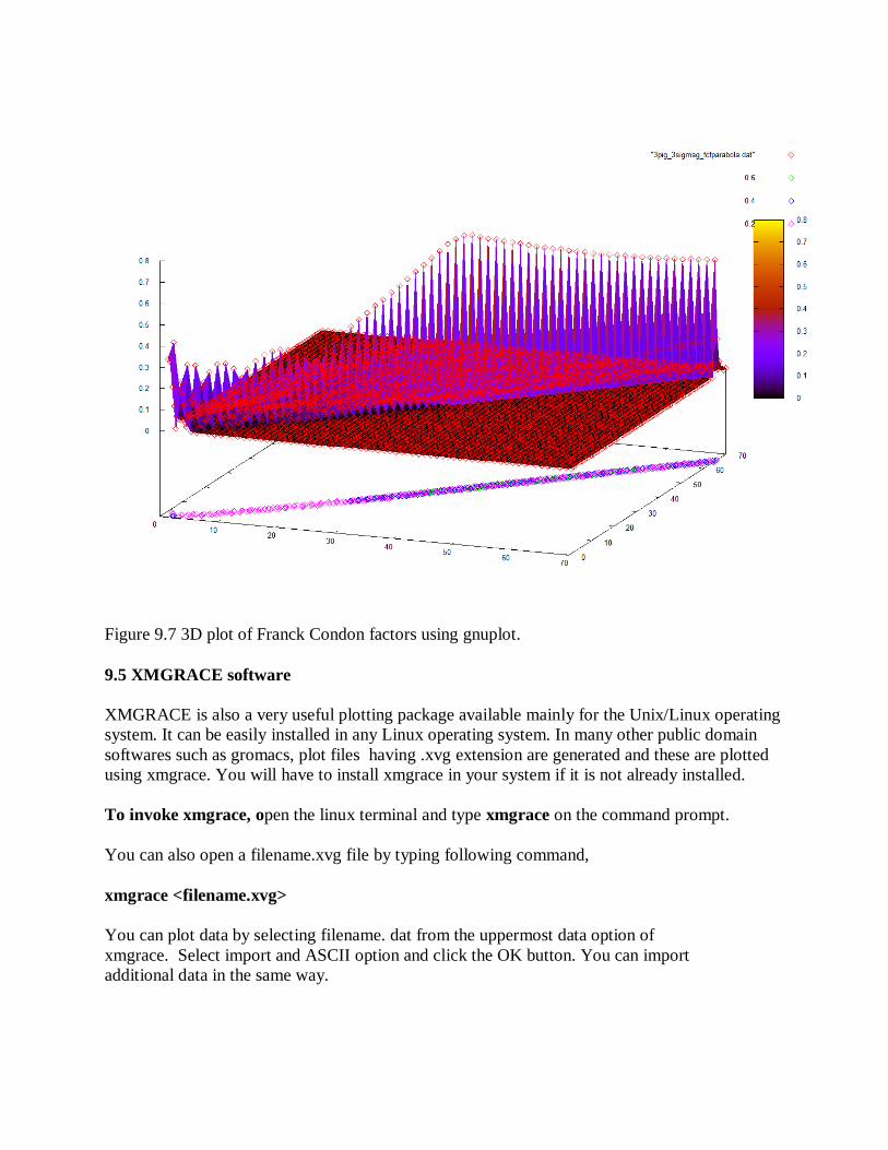
Figure 9.7 3D plot of Franck Condon factors using gnuplot.

9.5 XMGRACE software XMGRACE is also a very useful plotting package available mainly for the Unix/Linux operating system. It can be easily installed in any Linux operating system. In many other public domain softwares such as gromacs, plot files having .xvg extension are generated and these are plotted using xmgrace. You will have to install xmgrace in your system if it is not already installed. To invoke xmgrace, open the linux terminal and type xmgrace on the command prompt. You can also open a filename.xvg file by typing following command, xmgrace <filename.xvg> You can plot data by selecting filename. dat from the uppermost data option of xmgrace. Select import and ASCII option and click the OK button. You can import additional data in the same way.

For saving your plot, click on the file option at the top chose save as option give the desired name and save it in desired directory. It's conventional to use to suffix “.agr” for the file extension, e.g. filename.agr A post script (filename.ps) version of your plot can also be created by clicking on file menu and choosing print option. This will create a post script file (ps) with the same name as your filename.agr file e.g. filename.ps It is very easy to convert a post script file (filename.ps) to PDF or image file (e.g. ps to gif and ps to jpg etc etc) by using the convert command. On your terminal type the following. convert filename.ps to filename.pdf This will convert post script file to PDF file in the same directory. If you want to rotate your file you can do this by following command convert filename.ps –rotate 90 filename.pdf By studying Xmgrace Tutorials that are freely available on the Web, you can learn more details on i) Reading data from a file, ii) Axis Properties, iii) Set appearance iv) Graph appearance v) Operating on Data and vi) Saving, Printing, and Opening plots.

9.6 Summary

In this chapter, you were introduced to the computations of Fourier transforms of functions using the Scilab software, using the PlotDigitizer software in Linux to digitize continuous functions from any source that is available as a jpeg file, using the GNU plot softare in Linux to plot 3D plots and also the use Xmgrace software for graphics. These are very versatile softwares and are in the public domain. Reasonable practice with these softwares will help you considerably in report writing as well as in research activities.

9.7 Exercises: 1) Obtain cosine and Fourier transforms of biexponential functions such as Ae-Br + Ce-Dr for

suitable choices of parameters Am B, C and D. 2) Take a simple exponential plot and digitize it using the plotdigitizer software and then

check how well is the digitization by calculating the standard deviation between the actual function and het digitized function.

3) Use gnuplot to plot some elementary functions and also to fit a straight line and a parabola through a given set of datapoints

4) Practice using XMGRACE software