chapter 8 fourier transformscis.poly.edu/~mleung/cs4744/f04/ch12/fourier.pdf · chapter 8 fourier...

Chapter 8

Fourier Transforms

8.1 Touch-Tone DialingWe all use finite Fourier transforms every day without even knowing it. Cell phones,disc drives, DVDs and JPEGs all involve FFTs.

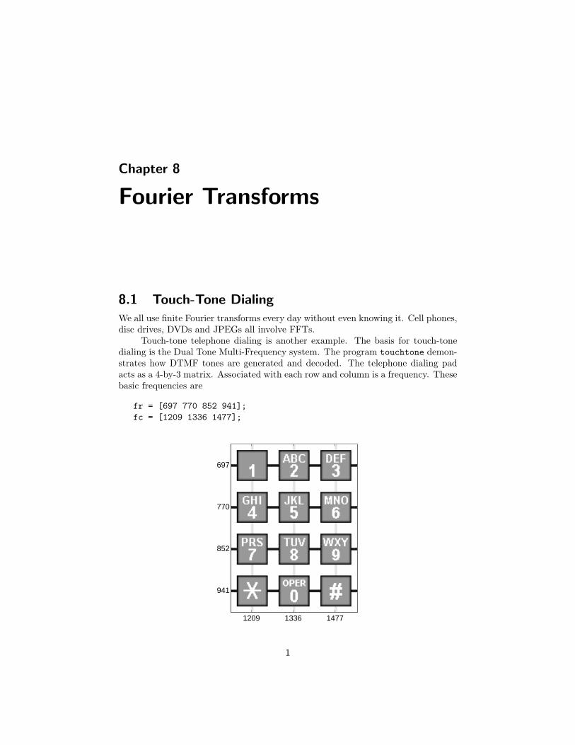
Touch-tone telephone dialing is another example. The basis for touch-tonedialing is the Dual Tone Multi-Frequency system. The program touchtone demon-strates how DTMF tones are generated and decoded. The telephone dialing padacts as a 4-by-3 matrix. Associated with each row and column is a frequency. Thesebasic frequencies are

fr = [697 770 852 941];fc = [1209 1336 1477];

1209 1336 1477

697

770

852

941

1

2 Chapter 8. Fourier Transforms

If s is a character that labels one of the buttons on the key pad, the corre-sponding row index k and column index j can be found with

switch scase ’*’, k = 4; j = 1;case ’0’, k = 4; j = 2;case ’#’, k = 4; j = 3;otherwise,

d = s-’0’; j = mod(d-1,3)+1; k = (d-j)/3+1;end

A key parameter in digital sound is the sampling rate.

Fs = 32768

A vector of points in the time interval 0 ≤ t ≤ 0.25 at this sampling rate is:

t = 0:1/Fs:0.25

The tone generated by the button in position (k,j) is obtained by superimposingthe two fundamental tones with frequencies fr(k) and fc(j).

y1 = sin(2*pi*fr(k)*t);y2 = sin(2*pi*fc(j)*t);y = (y1 + y2)/2;

If your computer is equipped with a sound card, the Matlab statement

sound(y,Fs)

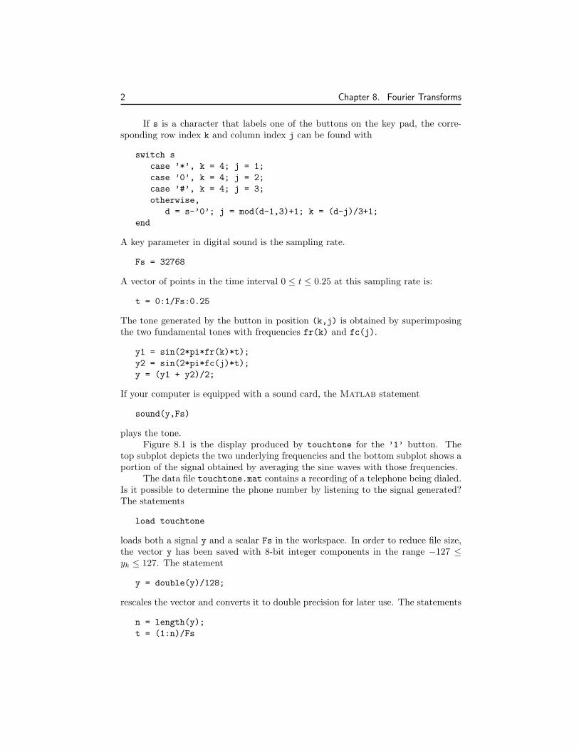
plays the tone.Figure 8.1 is the display produced by touchtone for the ’1’ button. The

top subplot depicts the two underlying frequencies and the bottom subplot shows aportion of the signal obtained by averaging the sine waves with those frequencies.

The data file touchtone.mat contains a recording of a telephone being dialed.Is it possible to determine the phone number by listening to the signal generated?The statements

load touchtone

loads both a signal y and a scalar Fs in the workspace. In order to reduce file size,the vector y has been saved with 8-bit integer components in the range −127 ≤yk ≤ 127. The statement

y = double(y)/128;

rescales the vector and converts it to double precision for later use. The statements

n = length(y);t = (1:n)/Fs

8.1. Touch-Tone Dialing 3

400 600 800 1000 1200 1400 16000

0.5

1

f(Hz)

1

0 0.005 0.01 0.015

−1

−0.5

0

0.5

1

t(secs)

Figure 8.1. The tone generated by the 1 button

1 2 3 4 5 6 7 8 9−1

0

1

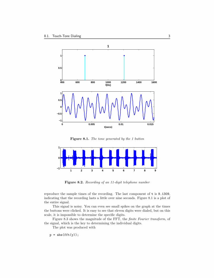
Figure 8.2. Recording of an 11-digit telephone number

reproduce the sample times of the recording. The last component of t is 9.1309,indicating that the recording lasts a little over nine seconds. Figure 8.1 is a plot ofthe entire signal.

This signal is noisy. You can even see small spikes on the graph at the timesthe buttons were clicked. It is easy to see that eleven digits were dialed, but on thisscale, it is impossible to determine the specific digits.

Figure 8.3 shows the magnitude of the FFT, the finite Fourier transform, ofthe signal, which is the key to determining the individual digits.

The plot was produced with

p = abs(fft(y));


600 800 1000 1200 1400 16000

200

400

600

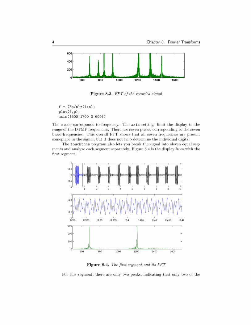
Figure 8.3. FFT of the recorded signal

f = (Fs/n)*(1:n);plot(f,p);axis([500 1700 0 600])

The x-axis corresponds to frequency. The axis settings limit the display to therange of the DTMF frequencies. There are seven peaks, corresponding to the sevenbasic frequencies. This overall FFT shows that all seven frequencies are presentsomeplace in the signal, but it does not help determine the individual digits.

The touchtone program also lets you break the signal into eleven equal seg-ments and analyze each segment separately. Figure 8.4 is the display from with thefirst segment.

1 2 3 4 5 6 7 8 9−1

−0.5

0

0.5

1

600 800 1000 1200 1400 16000

100

200

300

0.38 0.385 0.39 0.395 0.4 0.405 0.41 0.415 0.42−1

−0.5

0

0.5

1

Figure 8.4. The first segment and its FFT

For this segment, there are only two peaks, indicating that only two of the

8.2. Finite Fourier Transform 5

basic frequencies are present in this portion of the signal. These two frequenciescome from the ’1’ button. You can also see that the wave form of a short portionof the first segment is similar to the wave form that our synthesizer produces for the’1’ button. So, we can conclude that the number being dialed in touchtones startswith a 1. An exercise asks you to continue the analysis and identify the completephone number.

8.2 Finite Fourier TransformThe finite, or discrete, Fourier transform of a complex vector y with n elements isanother complex vector Y with n elements

Yk+1 =n−1∑

j=0

ωjkyj+1

where ω is a complex nth root of unity,

ω = e−2πi/n

This notation uses i for the complex unit,√−1, and j and k for indices that run

from 0 to n− 1. The subscripts j + 1 and k + 1 run from 1 to n, corresponding tothe range usually associated with linear algebra and Matlab vectors.

The Fourier transform can be expressed with matrix-vector notation

Y = Fy

where the finite Fourier transform matrix F has elements

fk+1,j+1 = ωjk

It turns out that F is nearly its own inverse. More precisely FH , the complexconjugate transpose of F , satisfies

FHF = nI

so

F−1 =1n

FH

This allows us to invert the Fourier transform.

y =1n

FHY

Hence

yj+1 =1n

n−1∑

k=0

Yk+1ωjk

where ω is the complex conjugate of ω

ω = e2πi/n


We should point out that this is not the only notation for the finite Fouriertransform in common use. The minus sign in the definition of ω after the first equa-tion sometimes occurs instead in the definition of ω used in the inverse transform.The 1/n scaling factor in the inverse transform is sometimes replaced by 1/

√n

scaling factors in both transforms.In Matlab, the Fourier matrix F could be generated for any given n by

omega = exp(-2*pi*i/n);j = 0:n-1;k = j’F = omega.^(k*j)

The quantity k*j is an outer product, an n-by-n matrix whose elements are theproducts of the elements of two vectors. However, the built-in function fft takesthe finite Fourier transform of each column of a matrix argument, so an easier, andquicker, way to generate F is

F = fft(eye(n))

The function fft uses a fast algorithm to compute the finite Fourier transform.The first “f” stands for both “fast” and “finite”. A more accurate name might beffft, but nobody wants to use that. We discuss the fast aspect of the algorithm ina later section.

8.3 fftgui

The GUI fftgui allows you to investigate properties of the finite Fourier transform.If y is a vector containing a few dozen elements,

fftgui(y)

produces four plots

real(y) imag(y)real(fft(y)) imag(fft(y))

You can use the mouse to move any of the points in any of the plots, and the pointsin the other plots respond.

Please run fftgui and try the following examples. Each illustrates someproperty of the Fourier transform. If you start with no arguments,

fftgui

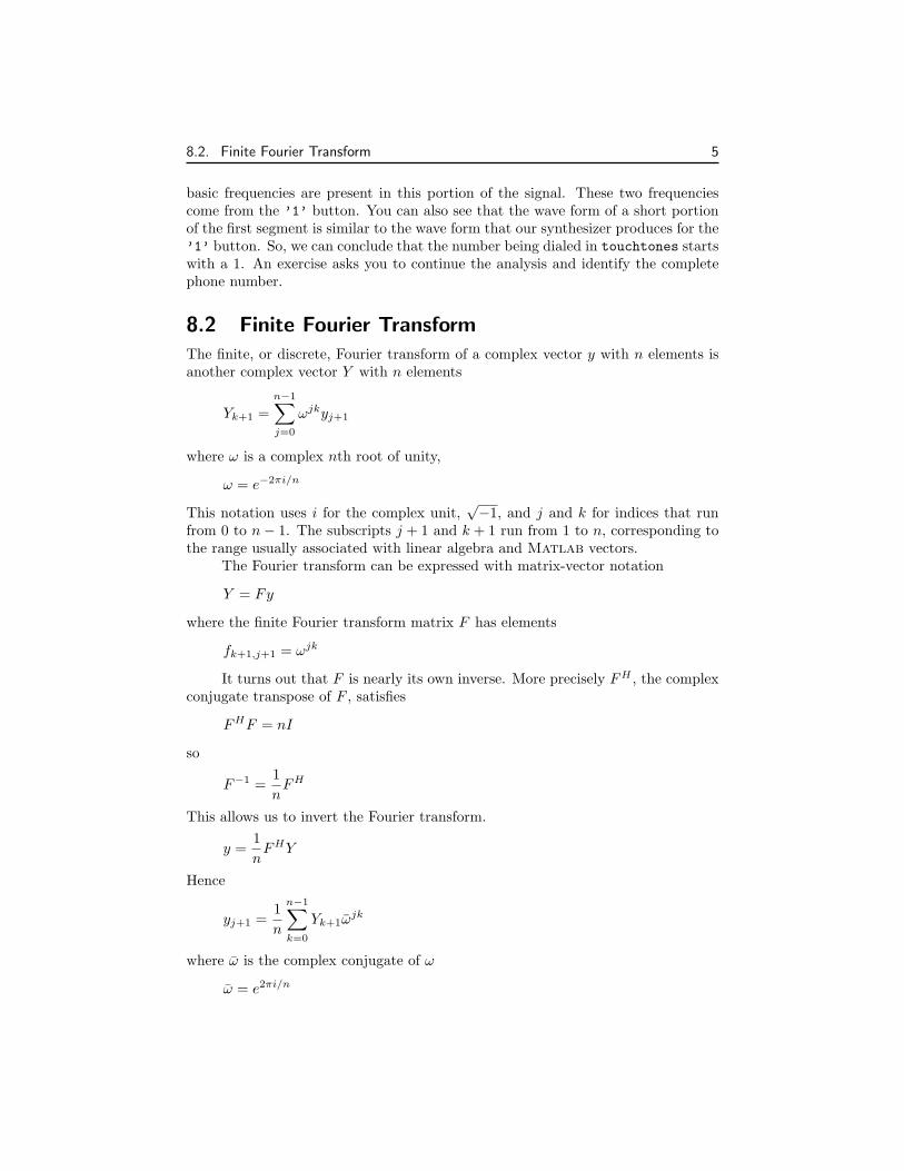
all four plots are initialized to zeros(1,32). Click your mouse in the upper lefthand corner of the upper left hand plot. You are taking the fft of the first unitvector, with one in the first component and zeros elsewhere. This should producefigure 8.5.

The real part of the result is constant and the imaginary part is zero. Youcan also see this from the definition

Yk+1 =n−1∑

j=0

yj+1e−2ijkπ/n, k = 0, . . . , n− 1

8.3. fftgui 7

real(y) imag(y)

real(fft(y)) imag(fft(y))

Figure 8.5. FFT of the first unit vector is constant

if y1 = 1 and y2 = · · · = yn = 0. The result is

Yk+1 = 1 · e0 + 0 + · · ·+ 0 = 1, for all k

Click y1 again, hold the mouse down, and move the mouse vertically. Theamplitude of the constant result varies accordingly.

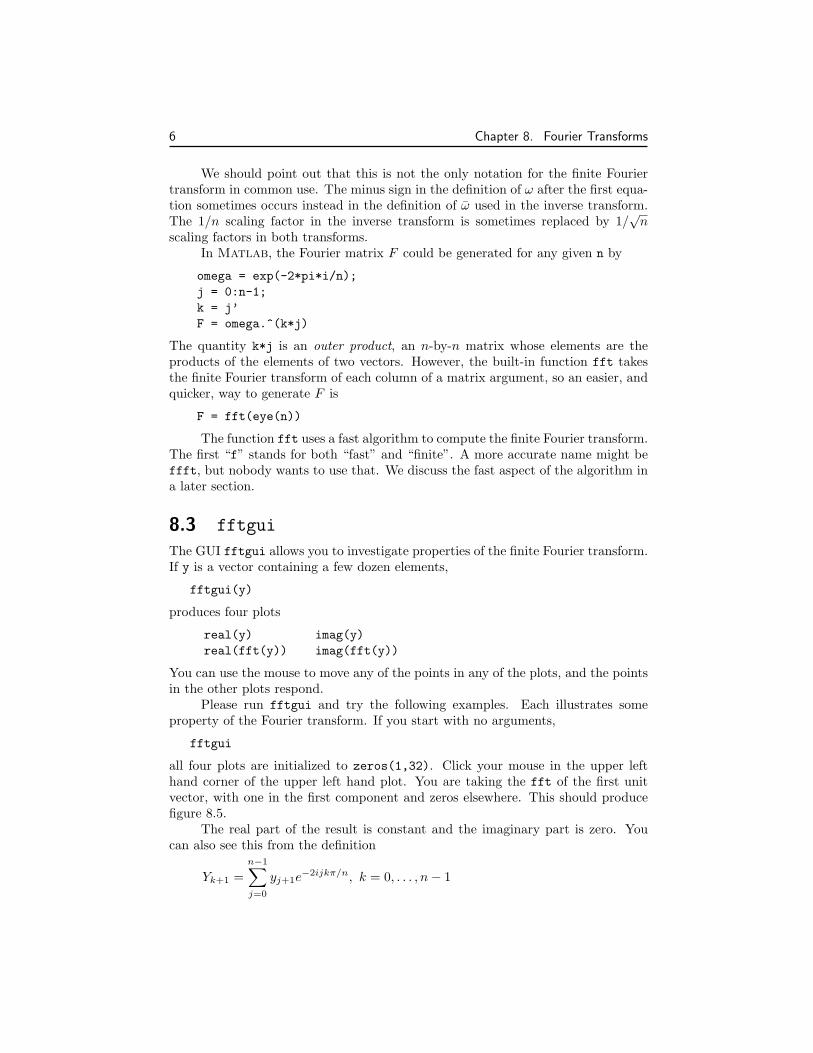
Next, try the second unit vector. Use the mouse to set y1 = 0 and y2 = 1.This should produce figure 8.6.

You are seeing the graph of

Yk+1 = 0 + 1 · e−2ikπ/n + 0 + · · ·+ 0

The nth root of unity can also be written

ω = cos δ − i sin δ, where δ = 2π/n

Consequently, for k = 0, · · · , n− 1,

real(Yk+1) = cos kδ, imag(Yk+1) = − sin kδ

We have sampled two trig functions at n equally spaced points in the interval0 ≤ x < 2π. The first sample point is x = 0 and the last sample point is x = 2π−δ.

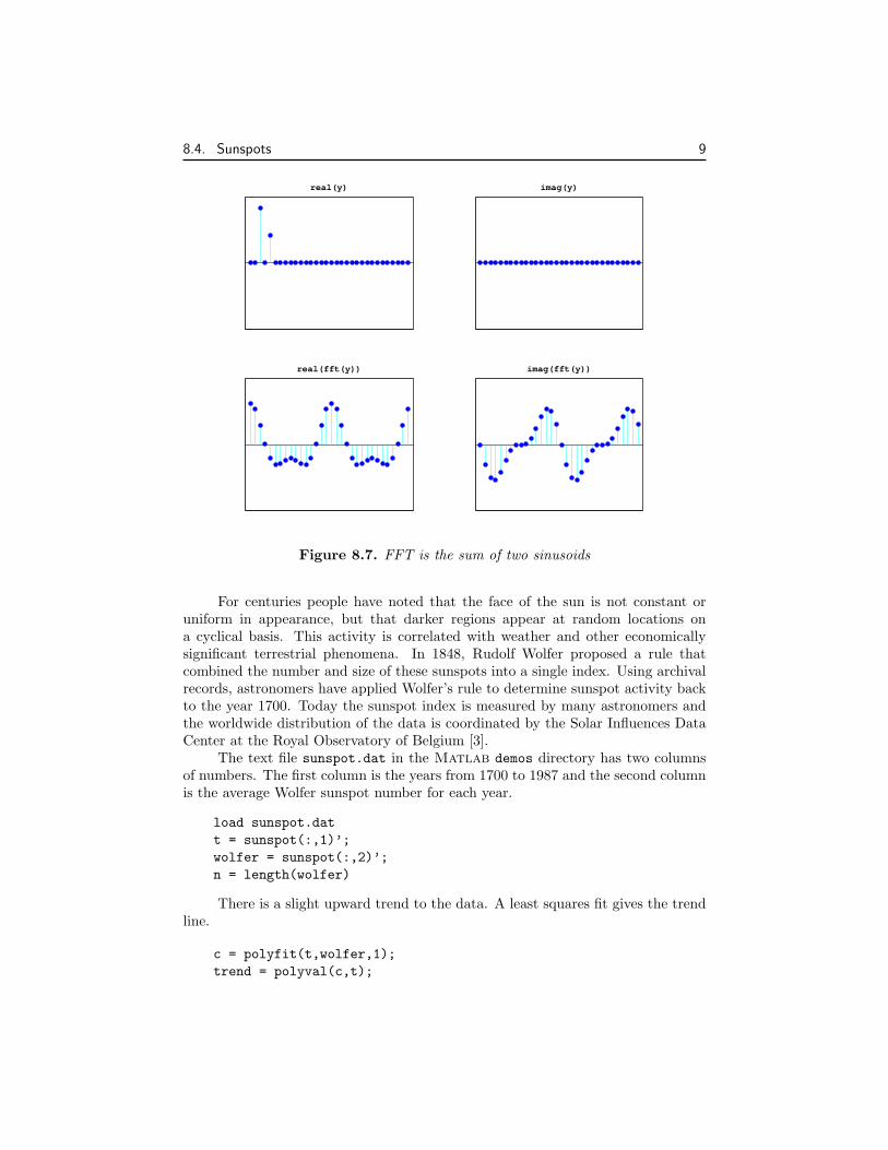
Now set y3 = 1 and vary y5 with the mouse. One snapshot is figure 8.6.We have graphs of

cos 2kδ + η cos 4kδ and − sin 2kδ − η sin 4kδ


real(y) imag(y)


Figure 8.6. FFT of the second unit vector is a pure sinusoid

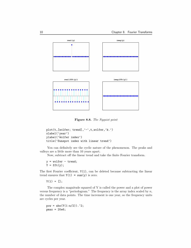
for various values of η = y5.The point just to the right of the midpoint of the x-axis is particularly impor-

tant. It is known as the Nyquist point. With the points numbered from 1 to n foreven n, it’s the point with index n

2 + 1. If n = 32, it’s point number 17. Figure 8.8shows that the fft of a unit vector at the Nyquist point is a sequence of alternating+1’s and −1’s.

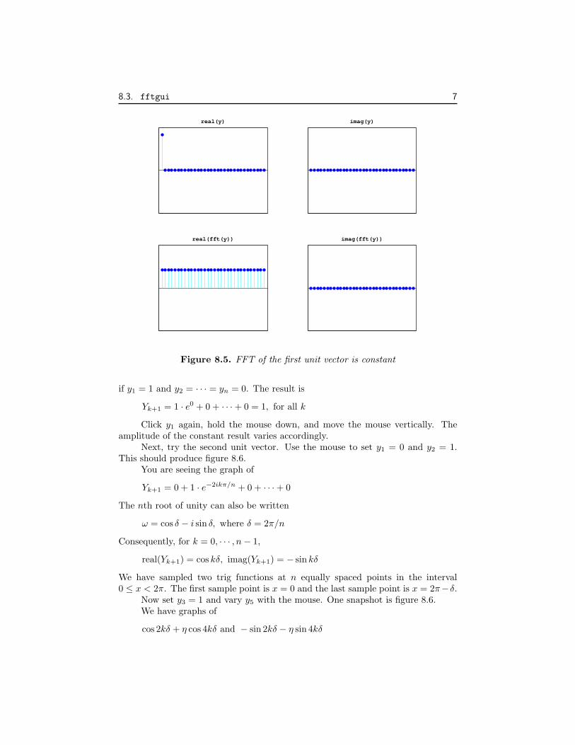
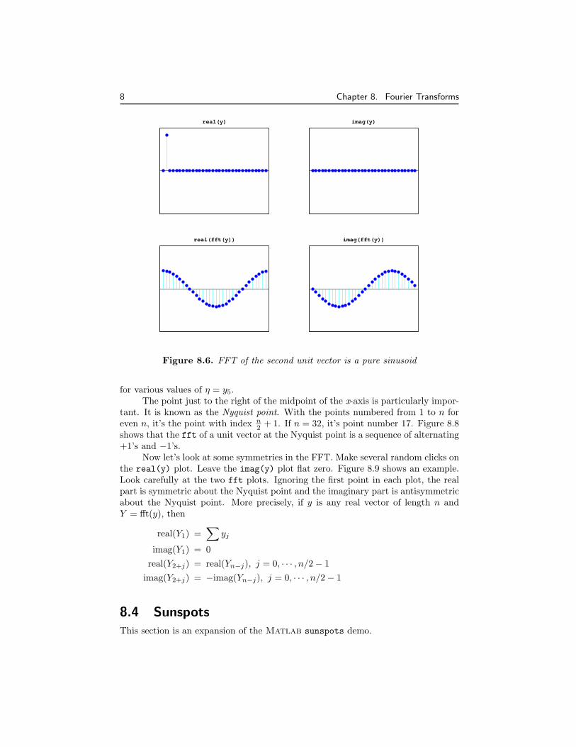
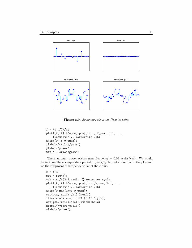
Now let’s look at some symmetries in the FFT. Make several random clicks onthe real(y) plot. Leave the imag(y) plot flat zero. Figure 8.9 shows an example.Look carefully at the two fft plots. Ignoring the first point in each plot, the realpart is symmetric about the Nyquist point and the imaginary part is antisymmetricabout the Nyquist point. More precisely, if y is any real vector of length n andY = fft(y), then

real(Y1) =∑

yj

imag(Y1) = 0real(Y2+j) = real(Yn−j), j = 0, · · · , n/2− 1

imag(Y2+j) = −imag(Yn−j), j = 0, · · · , n/2− 1

8.4 SunspotsThis section is an expansion of the Matlab sunspots demo.

8.4. Sunspots 9

real(y) imag(y)


Figure 8.7. FFT is the sum of two sinusoids

For centuries people have noted that the face of the sun is not constant oruniform in appearance, but that darker regions appear at random locations ona cyclical basis. This activity is correlated with weather and other economicallysignificant terrestrial phenomena. In 1848, Rudolf Wolfer proposed a rule thatcombined the number and size of these sunspots into a single index. Using archivalrecords, astronomers have applied Wolfer’s rule to determine sunspot activity backto the year 1700. Today the sunspot index is measured by many astronomers andthe worldwide distribution of the data is coordinated by the Solar Influences DataCenter at the Royal Observatory of Belgium [3].

The text file sunspot.dat in the Matlab demos directory has two columnsof numbers. The first column is the years from 1700 to 1987 and the second columnis the average Wolfer sunspot number for each year.

load sunspot.datt = sunspot(:,1)’;wolfer = sunspot(:,2)’;n = length(wolfer)

There is a slight upward trend to the data. A least squares fit gives the trendline.

c = polyfit(t,wolfer,1);trend = polyval(c,t);


real(y) imag(y)


Figure 8.8. The Nyquist point

plot(t,[wolfer; trend],’-’,t,wolfer,’k.’)xlabel(’year’)ylabel(’Wolfer index’)title(’Sunspot index with linear trend’)

You can definitely see the cyclic nature of the phenomenon. The peaks andvalleys are a little more than 10 years apart.

Now, subtract off the linear trend and take the finite Fourier transform.

y = wolfer - trend;Y = fft(y);

The first Fourier coefficient, Y(1), can be deleted because subtracting the lineartrend ensures that Y(1) = sum(y) is zero.

Y(1) = [];

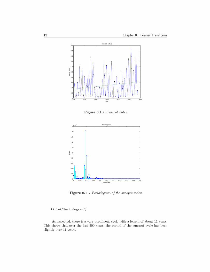
The complex magnitude squared of Y is called the power and a plot of powerversus frequency is a “periodogram.” The frequency is the array index scaled by n,the number of data points. The time increment is one year, so the frequency unitsare cycles per year.

pow = abs(Y(1:n/2)).^2;pmax = 20e6;

8.4. Sunspots 11

real(y) imag(y)


Figure 8.9. Symmetry about the Nyquist point

f = (1:n/2)/n;plot([f; f],[0*pow; pow],’c-’, f,pow,’b.’, ...

’linewidth’,2,’markersize’,16)axis([0 .5 0 pmax])xlabel(’cycles/year’)ylabel(’power’)title(’Periodogram’)

The maximum power occurs near frequency = 0.09 cycles/year. We wouldlike to know the corresponding period in years/cycle. Let’s zoom in on the plot anduse the reciprocal of frequency to label the x-axis.

k = 1:36;pow = pow(k);ypk = n./k(2:2:end); % Years per cycleplot([k; k],[0*pow; pow],’c-’,k,pow,’b.’, ...

’linewidth’,2,’markersize’,16)axis([0 max(k)+1 0 pmax])set(gca,’xtick’,k(2:2:end))xticklabels = sprintf(’%5.1f|’,ypk);set(gca,’xticklabel’,xticklabels)xlabel(’years/cycle’)ylabel(’power’)


1700 1750 1800 1850 1900 1950 20000

20

40

60

80

100

120

140

160

180

200

year

Wol

fer

inde

x

Sunspot activity

Figure 8.10. Sunspot index

0 0.05 0.1 0.15 0.2 0.25 0.3 0.35 0.4 0.45 0.50

0.2

0.4

0.6

0.8

1

1.2

1.4

1.6

1.8

2x 10

7

cycles/year

pow

er

Periodogram

Figure 8.11. Periodogram of the sunspot index

title(’Periodogram’)

As expected, there is a very prominent cycle with a length of about 11 years.This shows that over the last 300 years, the period of the sunspot cycle has beenslightly over 11 years.

8.5. Fast Finite Fourier Transform 13

144.0 72.0 48.0 36.0 28.8 24.0 20.6 18.0 16.0 14.4 13.1 12.0 11.1 10.3 9.6 9.0 8.5 8.00

0.2

0.4

0.6

0.8

1

1.2

1.4

1.6

1.8

2x 10

7

years/cycle

pow

er

Periodogram

Figure 8.12. Detail of periodogram shows 11 year cycle

8.5 Fast Finite Fourier TransformOne-dimensional FFTs with a million points and two-dimensional 1000-by-1000transforms are common. The key to modern signal and image processing is theability to do these computations rapidly.

Direct application of the definition

Yk+1 =n−1∑

j=0

ωjkyj+1, k = 0, . . . , n− 1

requires n multiplications and n additions for each of the n components of Y for atotal of 2n2 floating-point operations. This does not include the generation of thepowers of ω. A computer capable of doing one multiplication and addition everymicrosecond would require a million seconds, or about 11.5 days, to do a millionpoint FFT.

Several people discovered fast FFT algorithms independently and many peoplehave since contributed to their development, but it was a 1965 paper by John Tukeyof Princeton University and John Cooley of IBM Research that is generally creditedas the starting point for the modern usage of the FFT.

Modern fast FFT algorithms have computational complexity O(n log2n) in-stead of O(n2). If n is a power of 2, a one-dimensional FFT of length n requiresless than 3n log2n floating-point operations. For n = 220, that’s a factor of almost35,000 faster than 2n2. Even if n = 1024 = 210, the factor is about 70.

With Matlab 6.5 and a 700 MHz Pentium laptop, the time required forfft(x) if length(x) is 220 = 1048576 is about one second. The built-in fft func-tion is based on FFTW, “The Fastest Fourier Transform in the West,” developedat MIT by Matteo Frigo and Steven G. Johnson [1].


The key to the fast FFT algorithms is the double angle formula for trig func-tions. Using complex notation and

ω = ωn = e−2πi/n = cos δ − i sin δ

we have

ω22n = ωn

Written out in terms of separate real and imaginary parts, this is

cos 2δ = cos2δ − sin2δ

sin 2δ = 2 cos δ sin δ

Start with the basic definition.

Yk+1 =n−1∑

j=0

ωjkyj+1, k = 0, . . . , n− 1

Assume that n is even and that k ≤ n/2− 1. Divide the sum into terms with evensubscripts and terms with odd subscripts.

Yk+1 =∑

even j

ωjkyj+1 +∑

odd j

ωjkyj+1

=n/2−1∑

j=0

ω2jky2j+1 + ωk

n/2−1∑

j=0

ω2jky2j+2

The two sums on the right are components of the FFTs of length n/2 of the portionsof y with even and odd subscripts. In order to get the entire FFT of length n, wehave to do two FFTs of length n/2, multiply one of these by powers of ω, andconcatenate the results.

The relationship between an FFT of length n and two FFTs of length n/2 canbe expressed compactly in Matlab. If n = length(y) is even,

omega = exp(-2*pi*i/n);k = (0:n/2-1)’;w = omega .^ k;u = fft(y(1:2:n-1));v = w.*fft(y(2:2:n));

then

fft(y) = [u+v; u-v];

Now, if n is not only even, but actually a power of 2, the process can berepeated. The FFT of length n is expressed in terms of two FFTs of length n/2,then four FFTs of length n/4, then eight FFTs of length n/8 and so on until wereach n FFTs of length one. An FFT of length one is just the number itself. If

8.6. ffttx 15

n = 2p, the number of steps in the recursion is p. There is O(n) work at each step,so the total amount of work is

O(np) = O(n log2n)

If n is not a power of two, it is still possible to express the FFT of lengthn in terms of several shorter FFTs. An FFT of length 100 is two FFTs of length50, or four FFTs of length 25. An FFT of length 25 can be expressed in terms offive FFTs of length five. If n is not a prime number, an FFT of length n can beexpressed in terms of FFTs whose lengths divide n. Even if n is prime, it is possibleto embed the FFT in another whose length can be factored. We do not go into thedetails of these algorithms here.

The fft function in older versions of Matlab used fast algorithms if thelength was a product of small primes. Beginning with Matlab 6, the fft functionuses fast algorithms even if the length is prime. (See [1].)

8.6 ffttx

Our textbook function ffttx combines the two basic ideas of this chapter. If n isa power of 2, it uses the O(n log2n) fast algorithm. If n has an odd factor, it usesthe fast recursion until it reaches an odd length, then sets up the discrete Fouriermatrix and uses matrix-vector multiplication.

function y = ffttx(x)%FFTTX Textbook Fast Finite Fourier Transform.% FFTTX(X) computes the same finite Fourier transform% as FFT(X). The code uses a recursive divide and conquer% algorithm for even order and matrix-vector multiplication% for odd order. If length(X) is m*p where m is odd and% p is a power of 2, the computational complexity of this% approach is O(m^2)*O(p*log2(p)).

x = x(:);n = length(x);omega = exp(-2*pi*i/n);

if rem(n,2) == 0% Recursive divide and conquerk = (0:n/2-1)’;w = omega .^ k;u = ffttx(x(1:2:n-1));v = w.*ffttx(x(2:2:n));y = [u+v; u-v];

else% The Fourier matrix.j = 0:n-1;k = j’;


F = omega .^ (k*j);y = F*x;

end

8.7 fftmatrix

The n-by-n matrix F generated by the Matlab statement

F = fft(eye(n,n))

is a complex matrix whose elements are powers of the nth root of unity,

ω = e−2πi/n

The statement

plot(fft(eye(n,n)))

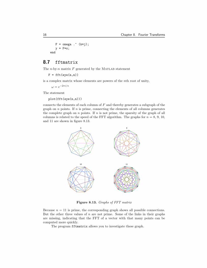
connects the elements of each column of F and thereby generates a subgraph of thegraph on n points. If n is prime, connecting the elements of all columns generatesthe complete graph on n points. If n is not prime, the sparsity of the graph of allcolumns is related to the speed of the FFT algorithm. The graphs for n = 8, 9, 10,and 11 are shown in figure 8.13.

8 9

10 11

Figure 8.13. Graphs of FFT matrix

Because n = 11 is prime, the corresponding graph shows all possible connections.But the other three values of n are not prime. Some of the links in their graphsare missing, indicating that the FFT of a vector with that many points can becomputed more quickly.

The program fftmatrix allows you to investigate these graph.

8.8. Other Fourier Transforms and Series 17

fftmatrix(n)

plots all the columns of the FFT matrix of order n.

fftmatrix(n,j)

plots only the j+1-st column.

fftmatrix

defaults to fftmatrix(10,4). In all cases, uicontrols allow n, j and the choicebetween one or all columns be changed.

8.8 Other Fourier Transforms and SeriesWe have been studying the finite Fourier transform, which converts one finite se-quence of coefficients into another sequence of the same length, n. The transformis

Yk+1 =n−1∑

j=0

yj+1e−2ijkπ/n, k = 0, . . . , n− 1

The inverse transform is

yj+1 =1n

n−1∑

k=0

Yk+1e2ijkπ/n, j = 0, . . . , n− 1

The Fourier integral transform converts one complex function into another.The transform is

F (µ) =∫ ∞

−∞f(t)e−2πiµtdt

The inverse transform is

f(t) =∫ ∞

−∞F (µ)e2πiµtdµ

The variables t and µ run over the entire real line. If t has units of seconds, then µhas units of radians per second. Both functions f(t) and F (µ) are complex valued,but in most applications the imaginary part of f(t) is zero.

Alternative units use ν = 2πµ, which has units of cycles or revolutions persecond. With this change of variable, there are no factors of 2π in the exponen-tials, but there are factors of 1/

√2π in front of the integrals, or a single factor of

1/(2π) in the inverse transform. Maple and the Matlab Symbolic Toolbox use thisalternative notation with the single factor in the inverse transform.

A Fourier series converts a periodic function into an infinite sequence of Fouriercoefficients. Let f(t) be the periodic function and let L be its period, so

f(t + L) = f(t) for all t


The Fourier coefficients are given by integrals over the period

cj =1L

∫ L/2

−L/2

f(t)e−2πijtdt, j = . . . ,−1, 0, 1, . . .

With these coefficients, the complex form of the Fourier series is

f(t) =∞∑

j=−∞cje

2πijt/L

A discrete time Fourier transform converts an infinite sequence of data valuesinto a periodic function. Let xk be the sequence, with the index k taking on allinteger values, positive and negative.

The discrete time Fourier transform is the complex valued periodic function

X(eiω) =∞∑

k=−∞xkeikω

The sequence can then be represented

xk =12π

∫ π

−π

X(eiω)e−ikωdω, k = . . . ,−1, 0, 1, . . .

The Fourier integral transform involves only integrals. The finite Fourier trans-form involves only finite sums of coefficients. Fourier series and the discrete timeFourier transform involve both integrals and sequences. It is possible to “morph”any of the transforms into any of the others by taking limits or restricting domains.

Start with a Fourier series. Let L, the length of the period, become infiniteand let j/L, the coefficient index scaled by the period length, become a continuousvariable, µ. Then the Fourier coefficients cj become the Fourier transform F (µ).

Again, start with a Fourier series. Interchanging the roles of the periodicfunction and the infinite sequence of coefficients leads to the discrete time Fouriertransform.

Start with a Fourier series a third time. Now restrict t to a finite numberof integral values, k, and restrict j to the same finite number of values. Then theFourier coefficients become the finite Fourier transform.

In the Fourier integral transform context, Parseval’s theorem says∫ +∞

−∞|f(t)|2dt =

∫ +∞

−∞|F (µ)|2dµ

This quantity is known as the total power in a signal.

8.9 Further ReadingVanLoan [4] describes the computational framework for the fast transforms. A pageof links at the FFTW Web site [2] provides useful information.

Exercises 19

Exercises8.1. What is the telephone number recorded in touchtone.mat and analyzed by

touchtone.m?8.2. Modify touchtone.m so that it can dial a telephone number specified by an

input argument, such as touchtone(’1-800-555-1212’)8.3. Our version of touchtone.m breaks the recording into a fixed number of

equally spaced segments, each corresponding to a single digit. Modify touchtoneso that it automatically determines the number and the possibly disparatelengths of the segments.

8.4. Investigate the use of the Matlab functions audiorecorder and audioplayer,or some other system for making digital recordings. Make a recording of aphone number and analyze it with your modified version of touchtone.m.

8.5. What relationship between n and j causes fftmatrix(n,j) to produce afive-point star? What relationship produces a regular pentagon?

8.6. el Nino. The climatological phenomenon el Nino results from changes in at-mospheric pressure in the southern Pacific ocean. The “Southern OscillationIndex” is the difference in atmospheric pressure between Easter Island andDarwin, Australia, measured at sea level at the same moment. The text fileelnino.dat contains values of this index measured on a monthly basis overthe 14 year period 1962 through 1975.Your assignment is to carry out an analysis similar to the sunspot exampleon the el Nino data. The unit of time is one month instead of one year. Youshould find there is a prominent cycle with a period of 12 months, and asecond, less prominent, cycle with a longer period. This second cycle showsup in about three of the Fourier coefficients, so it is hard to measure itslength, but see if you can make an estimate.

8.7. Train signal. The Matlab demos directory contains several sound samples.One of them is a train whistle. The statement

load train

gives you a long vector y and a scalar Fs whose value is the number of samplesper second. The time increment is 1/Fs seconds.If your computer has sound capabilities, the statement

sound(y,Fs)

plays the signal, but you don’t need that for this problem.The data does not have a significant linear trend. There are two pulses ofthe whistle, but the harmonic content of both pulses is the same.(a) Plot the data with time in seconds as the independent variable.(b) Produce a periodogram with frequency in cycles/second as the indepen-dent variable.(c) Identify the frequencies of the six peaks in the periodogram. You shouldfind that ratios between these six frequencies are close to ratios between


small integers. For example, one of the frequencies is 5/3 times another. Thefrequencies that are integer multiples of other frequencies are overtones. Howmany of the peaks are fundamental frequencies and how many are overtones?

8.8. Bird chirps. Analyze the chirp sound sample from the Matlab demos di-rectory. By ignoring a short portion at the end, it is possible to segment thesignal into eight pieces of equal length, each containing one chirp. Plot themagnitude of the FFT of each segment. Use subplot(4,2,k) for k = 1:8and the same axis scaling for all subplots. Frequencies in the range fromroughly 400 Hz to 800 Hz are appropriate. You should notice that one or twoof the chirps have distinctive plots. If you listen carefully, you should be ableto hear the different sounds.

Bibliography

[1] M. Frigo and S. G. Johnson, FFTW: An adaptive software architecture forthe FFT, Proc. 1998 IEEE Intl. Conf. Acoustics Speech and Signal Processing,3 (1998), pp. 1381–1384.http://www.fftw.org

[2] M. Frigo and S. G. Johnson, Links to FFT-related resources.http://www.fftw.org/links.html

[3] Solar Influences Data Center.http://sidc.oma.be

[4] C. Van Loan, Computational Frameworks for the Fast Fourier Transform,SIAM Publications, Philadelphia, PA., 1992, 273 pages.

21

chapter 8 fourier transformscis.poly.edu/~mleung/cs4744/f04/ch12/fourier.pdf · chapter 8 fourier...

Documents