Chapter 8Chapter 8

Curve FittingCurve Fitting

ContentContent

•Introduction•Linear Regression•Multidimensional unconstrained•Example

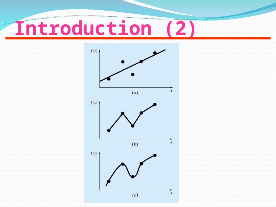
Introduction (1)Fit curves (curve fitting) to discrete data to obtain

intermediate estimates.

Two general approaches :Data exhibit a significant degree of scatter. The

strategy is to derive a single curve that represents the general trend of the data.

Data is very precise. The strategy is to pass a curve or a series of curves through each of the points.

Two types of engineering applications:Trend analysis (Extrapolation or Interpolation).Hypothesis testing.

Introduction (2)

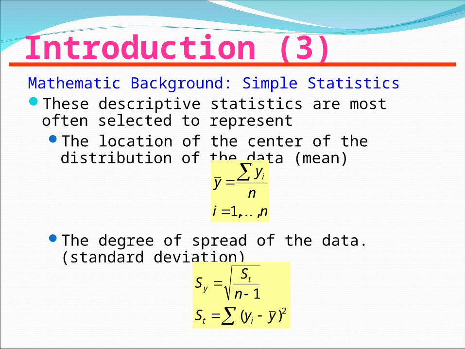
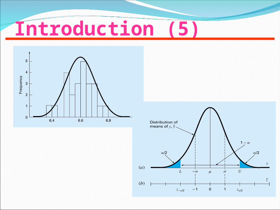
Introduction (3)Mathematic Background: Simple StatisticsThese descriptive statistics are most often selected to

representThe location of the center of the distribution of the data

(mean)

The degree of spread of the data. (standard deviation)

nin

yy i

,,1

2)(

1

yyS

n

SS

it

ty

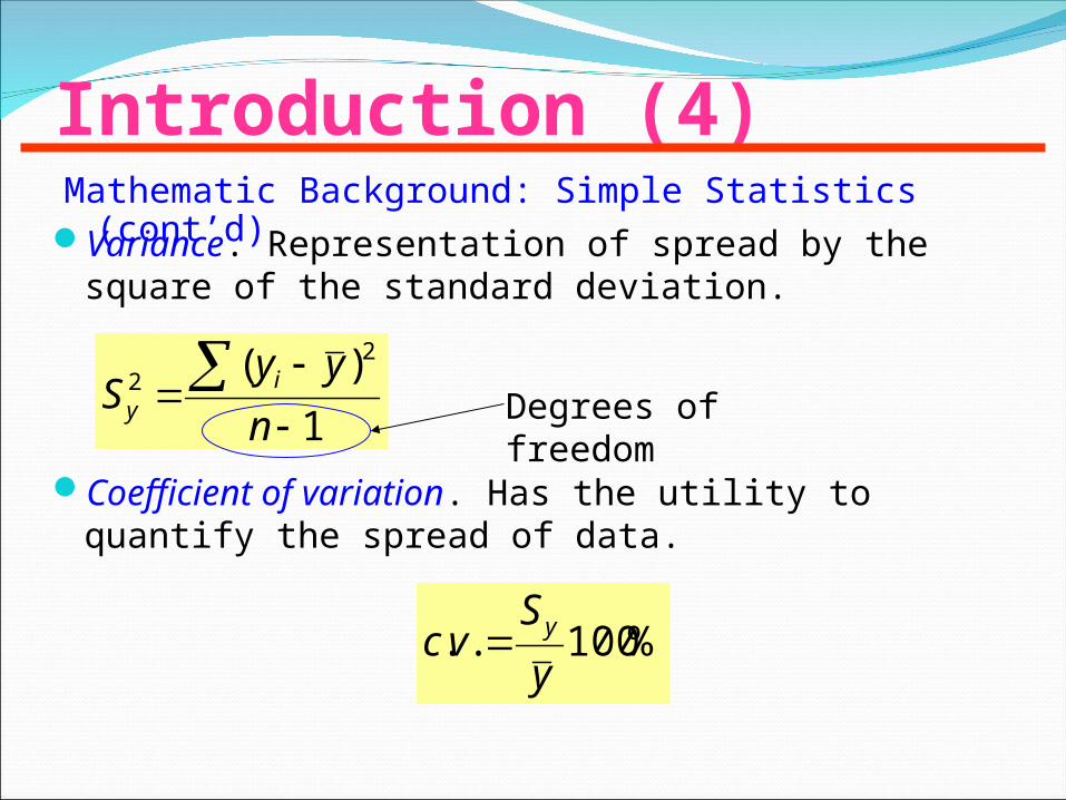
Introduction (4)Mathematic Background: Simple Statistics (cont’d)Variance. Representation of spread by the square of the

standard deviation.

Coefficient of variation. Has the utility to quantify the spread of data.

1

)( 22

n

yyS iy Degrees of freedom

%100..y

Svc y

Introduction (5)

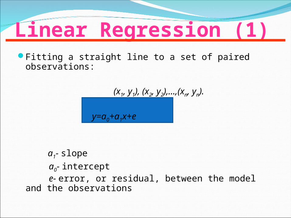
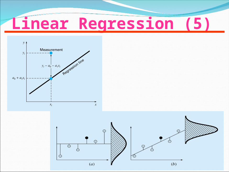
Linear Regression (1)Fitting a straight line to a set of paired observations:

(x1, y1), (x2, y2),…,(xn, yn).

y=a0+a1x+e

a1- slope

a0- intercept e- error, or residual, between the model and the observations

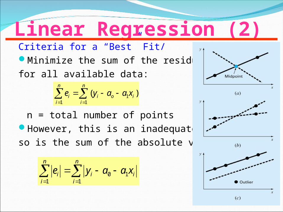
Linear Regression (2)Criteria for a “Best” Fit/Minimize the sum of the residual errors

for all available data:

n = total number of pointsHowever, this is an inadequate criterion,

so is the sum of the absolute values

n

iioi

n

ii xaaye

11

1

)(

n

iii

n

ii xaaye

110

1

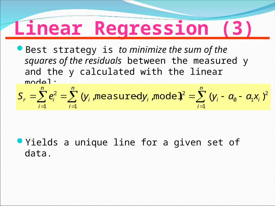
Linear Regression (3)Best strategy is to minimize the sum of the squares of the

residuals between the measured y and the y calculated with the linear model:

Yields a unique line for a given set of data.

n

i

n

iiiii

n

iir xaayyyeS

1 1

210

2

1

2 )()model,measured,(

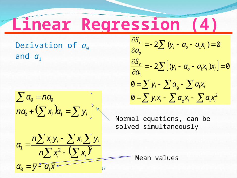
Linear Regression (4)

Chapter 17

210

10

11

1

0

0

0)(2

0)(2

iiii

ii

iioir

ioio

r

xaxaxy

xaay

xxaaya

S

xaaya

S

xaya

xxn

yxyxna

yaxna

naa

ii

iiii

ii

10

221

10

00

Normal equations, can be solved simultaneously

Mean values

Derivation of a0 and a1

Linear Regression (5)

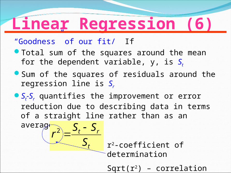
Linear Regression (6)“Goodness” of our fit/ IfTotal sum of the squares around the mean for the

dependent variable, y, is St

Sum of the squares of residuals around the regression line is Sr

St-Sr quantifies the improvement or error reduction due to describing data in terms of a straight line rather than as an average value.

t

rt

S

SSr

2

r2-coefficient of determination

Sqrt(r2) – correlation coefficient

Linear Regression (7)For a perfect fit

Sr=0 and r=r2=1, signifying that the line explains 100 percent of the variability of the data.

For r=r2=0, Sr=St, the fit represents no improvement.

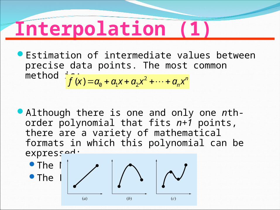
Interpolation (1)Estimation of intermediate values between precise data

points. The most common method is:

Although there is one and only one nth-order polynomial that fits n+1 points, there are a variety of mathematical formats in which this polynomial can be expressed:The Newton polynomialThe Lagrange polynomial

nnxaxaxaaxf 2

210)(

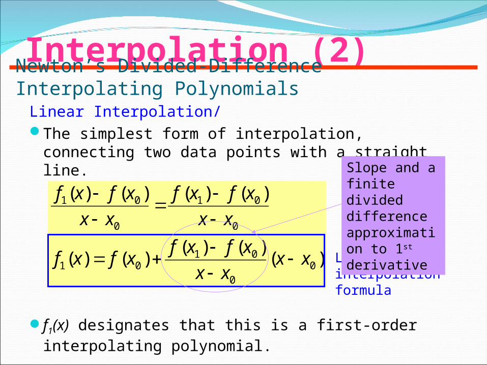
Interpolation (2)Newton’s Divided-Difference Interpolating Polynomials

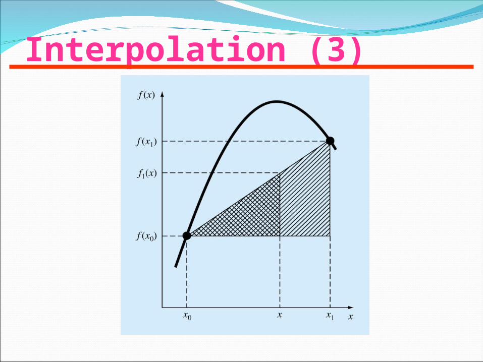
Linear Interpolation/The simplest form of interpolation, connecting two data

points with a straight line.

f1(x) designates that this is a first-order interpolating polynomial.

)()()(

)()(

)()()()(

00

0101

0

01

0

01

xxxx

xfxfxfxf

xx

xfxf

xx

xfxf

Linear-interpolation formula

Slope and a finite divided difference approximation to 1st derivative

Interpolation (3)

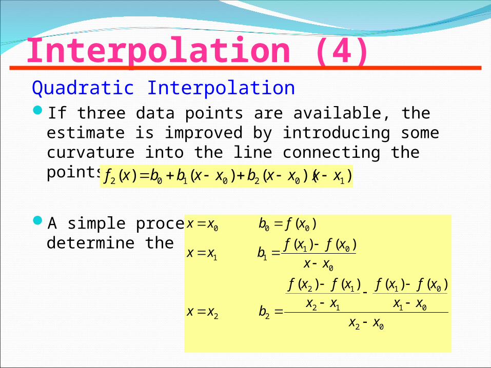
Interpolation (4)Quadratic InterpolationIf three data points are available, the estimate is

improved by introducing some curvature into the line connecting the points.

A simple procedure can be used to determine the values of the coefficients.

))(()()( 1020102 xxxxbxxbbxf

02

01

01

12

12

22

0

0111

000

)()()()(

)()(

)(

xx

xx

xfxf

xxxfxf

bxx

xx

xfxfbxx

xfbxx

Interpolation (5)

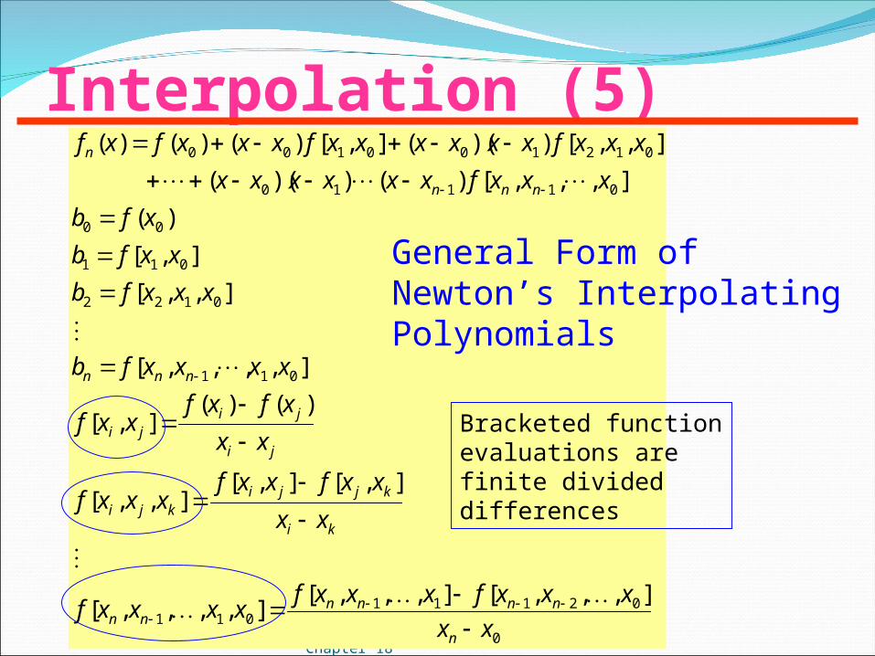
Chapter 180

02111011

011

0122

011

00

01110

012100100

],,,[],,,[],,,,[

],[],[],,[

)()(],[

],,,,[

],,[

],[

)(

],,,[)())((

],,[))((],[)()()(

xx

xxxfxxxfxxxxf

xx

xxfxxfxxxf

xx

xfxfxxf

xxxxfb

xxxfb

xxfb

xfb

xxxfxxxxxx

xxxfxxxxxxfxxxfxf

n

nnnnnn

ki

kjjikji

ji

jiji

nnn

nnn

n

Bracketed function evaluations are finite divided differences

General Form of Newton’s Interpolating Polynomials

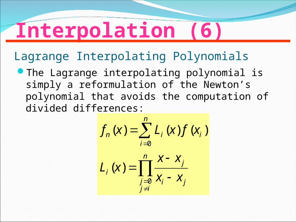
Interpolation (6)Lagrange Interpolating PolynomialsThe Lagrange interpolating polynomial is simply a

reformulation of the Newton’s polynomial that avoids the computation of divided differences:

n

ijj ji

ji

n

iiin

xx

xxxL

xfxLxf

0

0

)(

)()()(

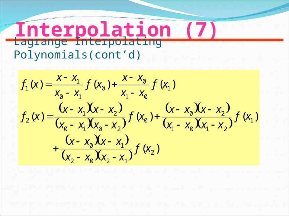
Interpolation (7)Lagrange Interpolating Polynomials(cont’d)

)(

)()()(

)()()(

21202

10

12101

200

2010

212

101

00

10

11

xfxxxx

xxxx

xfxxxx

xxxxxf

xxxx

xxxxxf

xfxx

xxxf

xx

xxxf

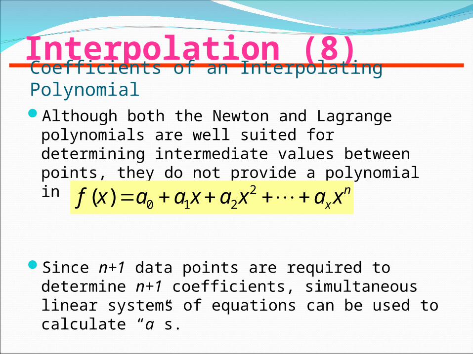
Interpolation (8)Coefficients of an Interpolating PolynomialAlthough both the Newton and Lagrange polynomials are

well suited for determining intermediate values between points, they do not provide a polynomial in conventional form:

Since n+1 data points are required to determine n+1 coefficients, simultaneous linear systems of equations can be used to calculate “a”s.

nxxaxaxaaxf 2

210)(

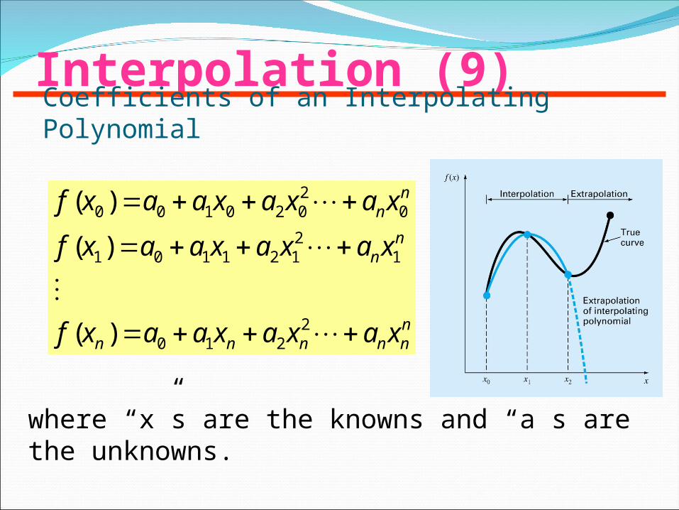
Interpolation (9)Coefficients of an Interpolating Polynomial

nnnnnn

nn

nn

xaxaxaaxf

xaxaxaaxf

xaxaxaaxf

2210

12121101

02020100

)(

)(

)(

where “x”s are the knowns and “a”s are the unknowns.