chapter 7: introduction to part ii: spatial econometrics

Chapter 7: Introduction to Part II: Spatial Econometrics

Zhenlin Yang

School of Economics, Singapore Management University

ECON6002: Panel Data and Spatial EconometricsTerm II, 2020-21

Z. L. Yang, SMU ECON6002, Term II 2020-21 1 / 45

Spatial econometrics

Spatial econometrics concerns spatial dependence or social interactionamong the geographical units, economic agents or social actors, such asneighbourhood effects, spillover effects, copy-catting, and peer effects.

It has received an increased attention by regional scientists,economists, econometricians, and statisticians.

Standard econometric techniques often fails in the presence of spatialinteractions. Spatial econometric models and methods extend thestandard ones to capture the spatial interactions.

They have been applied not only in specialized fields such as regionalscience, urban economics, real estate and economic geography,

but also increasingly in more traditional fields of economics, includingdemand analysis, labour economics, public economics, internationaleconomics, and agricultural and environmental economics.

And to finance as well, for issues, e.g., asset pricing with spatialinteraction (Kou, et al., 2017), stock market comovements, and more.


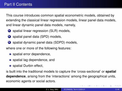
Part II Contents

This course introduces common spatial econometric models, obtained byextending the classical linear regression models, linear panel data models,and linear dynamic panel data models, namely,

1 spatial linear regression (SLR) models,2 spatial panel data (SPD) models,3 spatial dynamic panel data (SDPD) models,

where one or more of the following features:

spatial error dependence,

spatial lag dependence, and

spatial Durbin effect,

is built into the traditional models to capture the ‘cross-sectional’ or spatialdependence, arising from the ‘interactions’ among the geographical units,economic agents or social actors.


Spatial dependence is modeled by a spatial weight matrix or aconnectivity matrix, and a spatial parameter.

For each type model,

common inference methods, such as quasi-maximum likelihood(QML), M-estimation, and GMM, are introduced,

empirical illustrations are presented, and

Matlab routines are provided with which students can conduct theirown empirical analyses.

If time permits, recent advances on refined and robust inferences methodswill be discussed.

This chapter introduces common spatial econometric models and commonspatial weight matrices, presents some background knowledge on QML,M-, and GMM estimation methods, and discuss some popular applicationsof spatial models and recent developments in spatial software tools.


Brief History of Spatial Econometrics

The term spatial econometrics was coined by Jean Paelinck, a BelgiumEconometrician, in the early 1970s to designate a growing body of theregional science literature that dealt primarily with estimation and testingproblems encountered in the implementation of multiregional econometricmodels. See the Book: Anselin (1988, p.7).

The dependence among the cross-sectional units can be considered to lieat the core of the disciplines of the regional science and geography, asexpressed in Tobler’s (1979) first law of geography:

"everything is related to everything else, but nearthings are more related than distant things."

See also the books of Paelinck and Klaassen (1979), LeSage and Pace(1999), and Elhorst (2014).


While the concept of spatial dependence originated from the notion ofrelative space or relative location, which emphasizes the effect of distanceor neighborhood, the notation of space or location can easily be extendedbeyond the strict Euclidean space inducing

economic distance,

policy distance,

inter-personal distance,

social networks,

financial networks, etc.

Hence, spatial dependence is a phenomenon that exists in a wide rangeof applications in the social sciences and economics.


Spatial Linear Regression (SLR) Models

The SLR models extend the classical linear regression models:

Yn = Xnβ + un, (1)

by adding one or more of the following terms:1 spatial lag (SL) term: λ1W1nYn,2 spatial error (SE) term: un = λ2W2nun + vn,3 spatial Durbin (SD) term: W3nX ∗

n λ3,

to the right hand side (RHS) of (1), where

Yn (n × 1), Xn (n × p), β, and un have the usual interpretations,

X ∗n : a submatrix of Xn excluding the column of ones, etc,

Wrn, r = 1, 2, 3: known n × n spatial weight matrices, and

λ1, λ2, and λ3 are the parameters corresponding to, respectively, theSL, SE, and SD effects.


Spatial Panel Data (SPD) Models

The SPD models extend the classical panel data models:

Ynt = Xntβ + Znγ + µn + αt1n + unt , t = 1, . . . , T , (2)

by adding one or more of the following: λ1W1nYnt , λ2W2nunt , andλ3W3nX ∗

nt , being, respectively, the SL, SE and SD effects, where

Xnt : n × p matrix or time-varying regressors,

Zn: n × q matrix of time-invariant regressors,

µn is an n × 1 vector of unit-specific effects,

αt are the time-specific effects,

and the other quantities are similarly defined.

The µn and α′ts are called: (i) fixed effects if they are allowed to becorrelated with the time-varying regressors Xnt in an arbitrary manner; (ii)random effects if they are uncorrelated with Xnt ; or (iii) correlatedrandom effects if they are correlated with Xnt linearly.


Spatial Dynamic Panel Data (SDPD) Models

The SDPD models extend the classical dynamic panel data models:

Ynt = ρYn,t−1 + Xntβ + Znγ + µn + αt1n + unt , t = 1, . . . , T , (3)

by adding the SL, SE, or SD terms as in the SPD models. It can be furtherextended by adding a space-time effect λWnYn,t−1.

Challenges with the SDPD model:1 it incurs the incidental parameters problem (number of parameters

increase with the increase of sample size),2 it gives rise to the initial values problem (the distribution of the initial

observations Yn0 depends on the past values which areunobservables).

Remarks: For all the spatial econometric models, the spatial weightmatrices can be the same. The SL and SE effects can go for higher order.


Spatial Weight Matrix

Spatial weight matrix Wn = wij , i , j = 1, . . . , n is an n × n matrix thatmeasures the ‘connectivity’ among the n spatial units. The construction ofWn is a subject matter, depending on the actual problem considered.

Contiguity-based Weights: wij = 1 when units i and j are ‘neighbors’,and wi,j = 0 otherwise. Popular ones include:

Rook, Bishop, or Queen Contiguity: in a regular grid, theneighbors are those with common edge, or common vertex, orcombination of both, in analogy with the move of Rook, Bishop orQueen in the game of chess (Anselin, 1988, p.18);

Circular World: units immediate ahead or behind of a givenspatial unit are considered as neighbors of this unit, e.g., “5 aheadand 5 behind” (Kelejian and Prucha, 1999, p. 520);

Group Interaction: when n spatial units are naturally from Rgroups, the members within each group are neighbors, but themembers from different groups are not (Case, 1991; Lee, 2004).


Weights based on Physical Distance: The concept of neighbors can beextended to mean areal units with (i) common border, (ii) within a givencentroid distance of each other, or (iii) closest in terms of centroiddistance, etc., resulting Wn with elements 1 or 0 as above:

Common Border Weights: wij = 1 if units i and j share commonborder, and 0 otherwise;

K-Nearest Neighbors Weights: wij = 1 if units j(= 1, . . . , K )

are the K units closest to the unit i in terms of centroid distance;

Radial Distance Weights: wij = 1 for dij ≤ δ, where dij is thedistance between units i and j , and δ is the distance cutoff value,giving the distance-based contiguity.


Spatial weights wij can also be defined directly in terms of the actualdistance dij between units i and j , or in terms of the length ìj of thecommon boarder between units i and j :

Power Distance Weights: wij = d−αij , where α is any positive

exponent;

Exponential Distance Weights: wij = exp(−αdij), where α isa positive exponent;

Shared-Boundary Weights: wij = ìj/∑

k 6=i ìk , proportion of i − jboundary in the total boundary of unit i .


Weights based on Social or Economic Distance: Other specification ofspatial weights are possible as well (Anselin and Bera, 1998., p.244).

In sociometrics, the weights reflect whether or not two individualbelong to the same social network (Doreian, 1980).

In economics applications, the use of spatial weights based on“economic” distance has been suggested, among others, in Case etal. (1993). Specifically, they suggest to use weights of the form

wij = 1/|xi − xj |,

where xi and xj are observations on “meaningful” socioeconomiccharacteristics such as per capita income or percentage of thepopulation in a given racial or ethic group.


The final form of Wn is such that wii = 0, and Wn is row normalized, i.e.,each element is divided by its row sum.

Possible endogeneity in spatial weight matrix.Anselin and Bera (1998, p.244) made an important note:

in the standard estimation and testing problems, the weightsmatrix is taken to be exogenous. Therefore, indicators for thesocioeconomic weights should be chosen with great care toensure their exogeneity, unless their endogeneity is consideredexplicitly.


Roles of Spatial Terms

Consider a spatial contiguity-based weight matrix with n = 12 spatial units:

Wn =

8>>>>>>>>>>>>>>>>>>>>>>>><>>>>>>>>>>>>>>>>>>>>>>>>:

1 2 3 4 5 6 7 8 9 10 11 121 0 0 0 0 0 1/2 1/2 0 0 0 0 02 0 0 0 0 0 0 1/3 1/3 1/3 0 0 03 0 0 0 1/4 0 1/4 1/4 1/4 0 0 0 04 0 0 1/3 0 1/3 0 0 0 0 1/3 0 05 0 0 0 1/2 0 1/2 0 0 0 0 0 06 1/3 0 1/3 0 1/3 0 0 0 0 0 0 07 1/3 1/3 1/3 0 0 0 0 0 0 0 0 08 0 1/4 1/4 0 0 0 0 0 0 1/4 1/4 09 0 1/2 0 0 0 0 0 0 0 0 1/2 0

10 0 0 0 1/3 0 0 0 1/3 0 0 0 1/311 0 0 0 0 0 0 0 1/3 1/3 0 0 1/312 0 0 0 0 0 0 0 0 0 1/2 1/2 0

9>>>>>>>>>>>>>>>>>>>>>>>>=>>>>>>>>>>>>>>>>>>>>>>>>;


Spatial Error Mode: Yn = Xnβ + un, un = λWnun + vn.

The spatial connectivity matrix Wn given above implies that

u1 = (u6 + u7)/2 + v1,

u4 = (u3 + u5 + u10)/3 + v4, etc.

As un = (In − λWn)−1vn, if Var(vn) = σ2

v In, then we have,

Var(un) = σ2v [(In − λWn)

′(In − λWn)]−1, and thus,

Var(Yn) = σ2v [(In − λWn)

′(In − λWn)]−1.

However, E(Yn) = Xnβ, the same as the regular linear model.

Spatial error induces cross-sectional dependence in the disturbancesun, and thus changes the variance-covariance of the responses Yn, but itdoes not induce changes to the mean of Yn.


Spatial Lag Model: Yn = λWnYn + Xnβ + vn.

The spatial connectivity matrix Wn given above implies that

y1 = (y6 + y7)/2 + x ′1β + v1, etc.

y4 = (y3 + y5 + y10)/3 + x ′1β + v4, etc.

Since Yn = (In − λWn)]−1(Xnβ + vn), if Var(vn) = σ2

v In, then we have,

E(Yn) = (In − λWn)]−1Xnβ,

Var(Yn) = σ2u[(In − λWn)

′(In − λWn)]−1.

Therefore, spatial lag induces not only the so-called cross-sectionaldependence in Yn, but also the spatial effects on the means of Yn,i .

In the context of social networks, the latter is referred to as theendogenous spatial spillover effects.


Spatial Durbin Model: e.g., Yn = β01n + Xnβ1 + λWnXnγ + un.

For example, y1 = β0 + x1β1 + [(x6 + x7)/2]γ + u1.

The mean of the response y1 of the spatial unit 1 is affected not onlyby its own regressor value x1, but also by the regressor values of theneighboring spatial units 6 and 7, and similarly for the means of theresponses of the other spatial units.

The term Spatial Durbin first appeared in Anselin (1988, p. 40, p.111), for its analogy to the suggestion by Durbin (1960) for the timeseries case. In social interaction literature, it is referred to as thecontextual effects.

SD term induces the local effects (from the immediate neighbors), incontrast to the SL effect which induces the global effects (from theimmediate neighbors, neighbors of the immediate neighbors, etc.).

Change in, e.g., y1 caused by the change in x1 is referred to as thedirect effect; and changes in other y ′s caused by the change in x1

are referred to as the indirect effects that could be local or global.


Maximum Likelihood Estimation

The maximum likelihood (ML) estimator holds special place amongestimators (Cameron and Trivedi, 2005, p.139), as

it is the most efficient estimator among estimators which areconsistent and asymptotically normal, and

the principle behind the ML estimation lays out a foundation based onwhich many other more general methods are obtained such asquasi-ML estimation and M-estimation.

The likelihood principle, due to a pioneer statistician R. A. Fisher(1922), is to choose, as an estimator of parameter vector θ0, a value ofθ that maximizes the likelihood of observing the actual sample data.

The joint probability density function (pdf) of continuous randomobservations, or joint probability mass function (pmf) of discrete randomobservations, is the ‘likelihood’ for a particular sample to be observed.


Let f (y|θ) be the joint pdf or pmf of an n× 1 random vector Y indexed by avector θ of unknown parameters, given the exogenous regressors valuesX and exogenous spatial weights matrix W .

Now, fn(y|θ) is viewed as a function of θ and is denoted by Ln(θ|y) orsimply Ln(θ).

Then Ln(θ) is called the likelihood function of θ based on theobserved vector y on Y .

Maximizing Ln(θ) is equivalent to maximizing the loglikelihood`n(θ) = ln Ln(θ), and

θn = arg maxθ∈Θ `n(θ), (4)

is the so-called maximum likelihood estimator (MLE) of θ, where Θ

denotes the parameter space.

A simple interpretation could be: the observed vector y most likely‘came’ from the ‘population’ represented by f (y|θn).


There are some important properties of the ML principle.

Let Sn(θ) = ∂∂θ `n(θ), then, Sn(θ) is called score function.

At the true value θ0 of θ, Sn(θ0) is called efficient score.

For standard ML estimation problems, θn defined in (4) is equivalent to

θn = argSn(θ) = 0. (5)

Let ‘E’ denote the expectation with respect to the true pdf f (y|θ0), then

E[Sn(θ0)] = 0, (6)

The expectation of the outer product of the efficient score vector:

In ≡ In(θ0) = E[Sn(θ0)S′n(θ0)], (7)

is called the Fisher Information, commonly known as theinformation matrix or the expected information matrix.


The well-known information matrix equality (IME) holds under true `(θ):

−E[Hn(θ0)] = E[Sn(θ0)S′n(θ0)], (8)

where Hn(θ0) = ∂∂θ′ Sn(θ0), called the Hessian matrix. The negative

Hessian matrix is referred to as the Observed Information Matrix.

The proof of (6) goes as follows:

E[Sn(θ0)] =

∫Sn(θ0)f (y|θ0)dy

=

∫∂`n(θ0)

∂θf (y|θ0)dy

=

∫∂ ln f (y|θ0)

∂θf (y|θ0)dy =

∫∂

∂θf (y|θ0)dy

=∂

∂θ

∫f (y|θ0)dy =

∂

∂θ(1) = 0,

where differentiation and integration are assumed to be interchangeable,which is typically valid if the range of y does not depend on θ.


The proof of (8) goes as follows. Note that Hn(θ) = ∂2

∂θ∂θ′ `n(θ). We have

E[Hn(θ0)] =

∫∂2`n(θ0)

∂θ∂θ′f (y|θ0)dy

=

∫∂Sn(θ0)

∂θ′f (y|θ0)dy

=

∫∂

∂θ′[Sn(θ0)f (y|θ0)

]dy−

∫Sn(θ0)

[∂

∂θ′f (y|θ0)

]dy

=

∫∂

∂θ′[Sn(θ0)f (y|θ0)

]dy−

∫Sn(θ0)S′n(θ0)f (y|θ0)dy

=∂

∂θ′

∫Sn(θ0)f (y|θ0)dy−

∫Sn(θ0)S′n(θ0)f (y|θ0)dy

= 0− E[Sn(θ0)S′n(θ0)]

= −In.

Under some regularity conditions, we have

√n(θn − θ0)

D−→ N(0, limn→∞ nI−1n ). (9)


Quasi Maximum Likelihood Estimation

In practice, the true distribution of Y , say g(y|θ), is often unknown, the‘chosen’ distribution f (y|θ) can best be an approximation to g(y|θ). Thus,

Ln(θ) defined in terms of f (y|θ) is a wrong (quasi) likelihood function.Would maximizing the quasi-likelihood Ln(θ) still lead to a consistentestimator for θ0? Would the asymptotic normality result still hold?

It is well known that for a maximum likelihood type estimator, orM-estimator, to be consistent, it is necessary that

plim 1n Sn(θ0) = 0, (10)

which boils down by requiring that lim 1n E[Sn(θ0)] = 0.

However, this is not guaranteed if f (y|θ) is a misspecification.

Very interestingly, we can show that for a certain choice of f (y|θ) thatpartially specifies g(y|θ) in the sense that its first two momentsmatches these of g(y|θ), consistency can also be achieved.

One such a choice is the Gaussian likelihood.Z. L. Yang, SMU ECON6002, Term II 2020-21 24 / 45

Let Y ∼ (µn,Σn), i.e., the true joint pdf g(y|θ0) is known only up to the firsttwo moments: E(Y ) = µn ≡ µn(β0) and Var(Y ) = Σn ≡ Σn(γ0).

If the specified joint pdf is a normal, i.e., f (y|θ0) ∼ N[µ(β0),Σ(γ0)], thenthe quasi loglikelihood is

`n(θ) = −n2

ln(2π)− 12

ln |Σn(γ)| − 12

[y− µn(β)

]′Σ−1

n (γ)[y− µn(β)

], (11)

where , and θ = (β′, γ′)′. The quasi score function is

Sn(θ) =

µ′n(β)Σ−1

n (γ)[y− µn(β)

],

−Σ−1n (γ)Σnk (γ) +

[y− µn(β)

]′Σ−1

n (γ)Σnk (γ)Σ−1n (γ)

[y− µn(β)

],

for k = 1, . . . , dim(γ), where µ′n(β) = ∂∂β µ′n(β) and Σnk (γ) = ∂

∂γkΣn(γ).


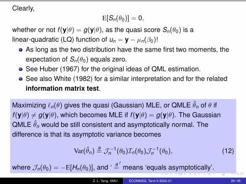
Clearly,E[Sn(θ0)] = 0,

whether or not f (y|θ) = g(y|θ), as the quasi score Sn(θ0) is alinear-quadratic (LQ) function of un = y− µn(β0)!

As long as the two distribution have the same first two moments, theexpectation of Sn(θ0) equals zero.See Huber (1967) for the original ideas of QML estimation.See also White (1982) for a similar interpretation and for the relatedinformation matrix test.

Maximizing `n(θ) gives the quasi (Gaussian) MLE, or QMLE θn of θ iff (y|θ) 6= g(y|θ), which becomes MLE if f (y|θ) = g(y|θ). The GaussianQMLE θn would be still consistent and asymptotically normal. Thedifference is that its asymptotic variance becomes

Var(θn)a= J−1

n (θ0)In(θ0)J−1n (θ0), (12)

where Jn(θ0) = −E[Hn(θ0)], and ‘a=′

means ‘equals asymptotically’.


Thus, in case that the true underlining distribution of a model isnonnormal, but normal (Gaussian) likelihood is used, the resultantestimator would still be consistent and asymptotically normal. This makesthe Gaussian QML estimation method very attractive.

Similar and more general results hold for other distributions from theexponential family (see Cameron and Trivedi, 2005, Sec. 5.7).Note that for models with SL effect WY , the usual OLS or GLSmethod cannot be applied due to the endogeneity in WY . However,as this type of endogeneity is of a ‘known form’, the ML or QMLmethod can still be applied.A limitation of the QML method is that it is inapplicable when modelcontains endogenous regressors of unknown form of endogeneity.GMM method is more general in handling the endogeneity issue.However, for spatial models with WY terms, WX are used to form IVsfor WY . Therefore, the existence of addition endogenous regressorswould cause a major problem.


M-Estimation

The term ‘M-estimator’ was coined by Huber (1964) to mean the maximumlikelihood type estimator (see also Huber, 1969). An M-estimator θn of ap × 1 vector of parameters θ is defined in two ways:

(a) as the solution of a maximization problem and(b) as the root of a set of estimating equations.

In case (a), θn is defined as

θn = arg maxθ∈Θ Qn(θ), (13)

For real valued, random criterion function Qn(θ).

In case (b), θn is defined as

θn = argΨn(θ) = 0, (14)

for p × 1 vector-valued estimating function Ψn(θ).Z. L. Yang, SMU ECON6002, Term II 2020-21 28 / 45

The asymptotic behavior of the M-estimator θn is similar to that of the QMLestimator. In particular, it is consistent and asymptotically normal.

Under regularity conditions, the M-estimator θn is such that θnp−→ θ0, and

√n(θn − θ0)

D−→ N[0, limn→∞

nΣ−1n (θ0)Γn(θ0)Σ

−1n (θ0)],

where Γn(θ0) = Var[Ψn(θ0)] and Σn(θ0) = −E[ ∂∂θ′ Ψn(θ0)].

The original formulation of the M-estimation is in terms of Qn or Ψn

which is the sum of n independent quantities. However, this can begeneralized to allow either function to have more general forms to suitfor the estimation of more general models such as the spatialeconometric models considered in this course.See van der Vaart (1998) for more general formulations ofM-estimation strategy, including the methods for proving itsasymptotic properties.See also White (1994) for the relevant asymptotic methods.


Generalized Method of Moments Estimation

The generalized method of moments (GMM), developed by Lars PeterHansen in 1982 as a generalization of the method of moments which wasintroduced by Karl Pearson in 1894, is a generic method for estimatingparameters in statistical models.

Usually it is applied in the context of semiparametric models, wherethe parameter of interest is finite-dimensional, whereas the full shapeof the distribution function of the data may not be known, andtherefore maximum likelihood estimation is not applicable.

The method requires that certain moment conditions be specifiedfor the model. These moment conditions are functions of the modelparameters and the data, such that their expectation is zero at thetrue values of the parameters.

The GMM method then minimizes a certain norm of the samplemoment conditions.


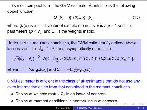
In its most compact form, the GMM estimator θn minimizes the followingobject function:

Qn(θ) = g′n(θ)Ωngn(θ), (15)

where gn(θ) is a r × 1 vector of sample moments, θ is a p × 1 vector ofparameters (p ≤ r), and Ωn is the weights matrix.

Under certain regularity conditions, the GMM estimator θn defined aboveis consistent, i.e., θn

p−→ θ0, and asymptotically normal, i.e.,

√n(θn − θ0)

D−→ N[0, limn→∞

n(Σ′nΩnΣn)−1(Σ′nΩnΓnΩnΣn)(Σ

′nΩnΣn)

−1],

where Γn = Var[gn(θ0)] and Σn = −E[ ∂∂θ′ gn(θ0)].

GMM estimator is efficient in the class of all estimators that do not use anyextra information aside from that contained in the moment conditions.

Choice of weights matrix Ωn is an issue of concern.

Choice of moment conditions is another issue of concern.


Optimal GMM. If Γn is ‘known’, then one can choose Ωn = Γ−1n . In this

case, the asymptotic variance-covariance (VC) matrix of the GMMestimator simplifies to

(ΣnΓ−1n Σn)

−1,

a similar form to the asymptotic VC matrix of an M-estimator.

When r = p, the model is said to be just-identified. In this case, Ωn issimply taken to be the identity matrix, and the GMM estimator becomesthe method of moments (MM) estimator defined as

θn = argg′n(θ) = 0. (16)

Clearly, the MM estimator is also the M-estimator defined earlier. In thiscase, Σn is also invertible, and the asymptotic VC matrix can be written asΣ−1

n ΓnΣ−1n .


Selected Applications

Neighborhood Crime. In illustrating the applications of spatialcross-sectional models, Anselin (1988, p.187) used the neighborhoodcrime data corresponding to 49 contiguous neighborhood in Columbus,Ohio, in 1980. These neighborhood correspond to census tracts, oraggregates of a small number of census tracts, where

Crime: the combined total of residential burglaries and vehicle theftsper thousand household in the neighborhood (the response variable).

Income and House: the explanatory variables representing incomeand housing values in thousand dollars.

East: a dummy variable indicates whether the ‘neighborhood’ in theeast or west of a main north-south transportation axis.

In addition, the neighborhood centroid coordinates (X and Y) are alsogiven, as well as the list of neighbors of each spatial unit(neighborhood) that gives a first-order contiguity spatial weight matrix.


Boston House Price. The data, given by Harrison and Rubinfeld (1978),and corrected and augmented with longitude and latitude by Gilley andPace (1996), contains 506 observations (1 observation per census tract)from Boston Metropolitan Statistical Area, and can be found in R (sedep).The response variable MEDV and 13 explanatory variables are:

MEDV: median value (corrected) of owner-occupied homes in 1000’s;

crime: per capita crime rate by town;

zoning: proportion of residential land zoned for lots over 25,000square feet;

industry: proportion of non-retail business acres per town;

charlesr: Charles River dummy variable (= 1 if tract bounds river);

nox: nitric oxides concentration (parts per 10 million);

room: average number of rooms per dwelling;

houseage: proportion of owner-occupied units built prior to 1940;

distance: weighted distances to five Boston employment centres;

access: index of accessibility to radial highways;


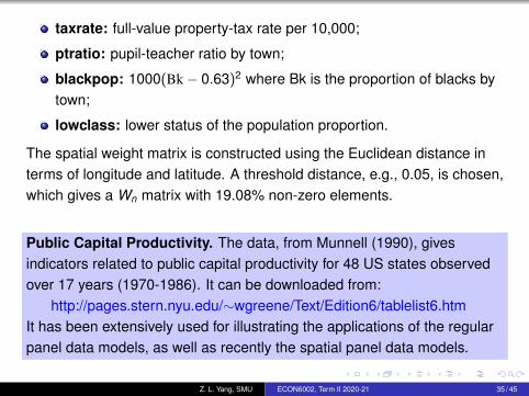
taxrate: full-value property-tax rate per 10,000;

ptratio: pupil-teacher ratio by town;

blackpop: 1000(Bk− 0.63)2 where Bk is the proportion of blacks bytown;

lowclass: lower status of the population proportion.

The spatial weight matrix is constructed using the Euclidean distance interms of longitude and latitude. A threshold distance, e.g., 0.05, is chosen,which gives a Wn matrix with 19.08% non-zero elements.

Public Capital Productivity. The data, from Munnell (1990), givesindicators related to public capital productivity for 48 US states observedover 17 years (1970-1986). It can be downloaded from:

http://pages.stern.nyu.edu/∼wgreene/Text/Edition6/tablelist6.htmIt has been extensively used for illustrating the applications of the regularpanel data models, as well as recently the spatial panel data models.


In Munnel (1990), the empirical model specified is a Cobb-Douglasproduction function of the form:

ln Y = β0 + β1 ln K1 + β2 ln K2 + β3 ln L + β4Unemp + ε,

with state specific fixed effects, where

Y is the gross social product of a given state,

K1 is public capital,

K2 is private capital,

L is labour input and Unemp is the state unemployment rate.

The spatial weights matrix W takes a contiguity form with its (i , j)thelement being 1 if states i and j share a common border, otherwise 0.The final W is row normalised.

For models with more than one spatial term, the corresponding W ′sare taken to be the same.

This model can be extended by adding the dynamic effect and one ormore spatial effects.


Cigarette Demand. This is another well known panel data that has beenapplied under various panel data model frameworks, non-spatial orspatial, fixed effects or random effects, static or dynamic. In particular, thedemand equations for cigarettes for United States were estimated, basedon a panel of 46 states over 30 time periods (1963-1992), given asCIGAR.TXT on the Wiley web site associated with book of Baltagi (2013).

Y = Cigarette sales in packs per capita (the response variable).

X1 = Price per pack of cigarettes;

X2 = Population (Pop);

X3 = Population above the age of 16;

X4 = Consumer price index with (1983=100);

X5 = Per capita disposable income;

X6 = Minimum price in adjoining states per pack of cigarettes.

Several time dummies corresponding to the major policy interventionsin 1965, 1968 and 1971 can be added into the model.

Spatial weights can be the first-order contiguity matrix.Z. L. Yang, SMU ECON6002, Term II 2020-21 37 / 45

Homicide Rate. Spatial patterns of homicide in counties in southernstates of the United States are studied by Messener et al. (2000). Thedata on homicide rate (hrate) were collected for the years 1960, 1970,1980, and 1990. The variables are:

_ID: Spatial-unit ID_CX: x-coordinate of area centroid_CY: y-coordinate of area centroidyear: Yearcname: County namesname: State namesfips: State FIPS codecfips: County FIPS codefips: Combined state and county FIPS codesouth: Located in the south (1=yes)hrate: Homicide rate per 100,000hcount: Homicide count three years average centered on yearpopulation: County population


ln_population: Log of population size

ln_pdensity: Log of population density

psize: Population size index

age: Median age

black: Percentage of black

femalehead: Percentage of female-headed households

divorce: Divorce rate

unemployment: Unemployment rate

ln_income: Log of median of family income

poverty: Percentage of families below poverty line

gini: Gini index of family income inequality

edeprivation: Economic deprivation index

The data has been extensively used in STATA 16 for illustrating themethods for SLR models based on 1990 data, and the methods for SPDmodels based all four years data.


Spatial Software Tools – STATA

STATA provides estimation and inferences methods for SLR and SPDmodels, but not for SDPD models. See Stata manual sp.pdf for details.The main commands, spxtregress and spxtregress, fit SLR andSPD models, respectively. The availability of shape file (name_shp.dta),beside the regular .dta file, facilitates the construction of various spatialweight matrices (contiguity or inverse distance).

The spatial weight matrix can be directly entered or imported.

Other major commands include:

spset: declares data to be Sp spatial data.

spmatrix: creates, imports, manipulates and exports W spatialweight matrices.

spmatrix import: imports spatial weight matrix from a text file.

spmatrix export: exports spatial weight matrix in standard format.


Spatial Software Tools – Others

The Matlab codes provided in this course are sufficient for the applicationsof common spatial econometrics models. Other software includes:

GeoDa (https://spatial.uchicago.edu/geoda) is a free softwarepackage that conducts spatial data analysis, geovisualization, spatialautocorrelation and spatial modeling.

spdep (https://cran.r-project.org/web/packages/spdep/index.html) isan R package containing a collection of R functions for spatialanalyses (spdep.pdf, book.pdf).

The website: https://spatial-panels.com/software/, lists some spatialsoftware codes for spatial panel data modelling.

See the “Handbook of Applied Spatial Analysis: Software tools,Methods and Applications” for a comprehensive coverage on spatialsoftware, methods and applications.


References

Anselin, L., 1988. Spatial econometrics: Methods and models.Dordrecht: Kluwer Academic Publishers.

Anselin L., Bera, A. K., 1998. Spatial dependence in linear regressionmodels with an introduction to spatial econometrics. In: Handbook ofApplied Economic Statistics, Edited by Aman Ullah and David E. A.Giles. New York: Marcel Dekker.

Baltagi, B. H., 2013. Econometric Analysis of Panel Data, 5th edition.John Wiley & Sons Ltd.

Case, A. C., 1991. Spatial Patterns in Household Demand.Econometrica 59, 953-965.

Case, A. C., Rosen, H. S., Hines, J. R., 1993. Budget Spillovers andFiscal Policy Interdependence: Evidence from the States. Journal ofPublic Economics 52, 285-307.

Cameron, A. C., Trivedi, P. K., 2005. Microeconometrics: Methodsand Applications. Cambridge University Press.


Doreian, P., 1980. Linear models with spatially distributed data:spatial disturbances and spatial effects. Sociology Methods andResearch 9, 29-60.Durbin, J. 1960. Estimation of parameters in time-series regressionmodels. Journal of the Royal Statistical Soceity B 22, 139-153.Elhorst, J. P., 2014. Spatial Econometrics From Cross-Sectional Datato Spatial Panels. Springer.Fisher, R. A., 1922. On mathematical foundation of theoreticalstatistics. Philosophical Transactions of the Royal Society of LondonA 222, 309-368.Gilley, O. W., Pace, R. K., 1996. On the Harrison and Rubinfeld Data.Journal of Environmental Economics and Management 31, 403-405.Hansen, L. P., 1982. Large sample properties of generalized methodof moments estimators. Econometrica 50, 1029-1054.Harrison, D., Rubinfeld, D. L., 1978. Hedonic housing prices and hedemand for clear air. Journal of Environmental Economics andManagement 5, 81-102.


Huber, P. J., 1964. Robust estimation of a location parameter. Annalsof Mathematical Statistics 35, 73-101.

Huber, P. J., 1967. The behavior of maximum likelihood estimatesunder nonstandard conditions. Proc. Fifth Berkeley Symp. onMathematical Statistics and Probability, vol. 1, pp. 221-233.

Kelejian H. H., Prucha, I. R., 1999. A generalized moments estimatorfor the autoregressive parameter in a spatial model. InternationalEconomic Review 40, 509-533.

Kou S., Peng, X, Zhong, H., 2017. Asset Pricing with SpatialInteraction. Management Science, Published online in Articles inAdvance 06 Feb 2017.

Lee, L. F., 2004. Asymptotic distributions of quasi-maximum likelihoodestimators for spatial autoregressive models. Econometrica 72,1899-1925.

LeSage, J., Pace, R.K., 2009. Introduction to Spatial Econometrics.London: CRC Press, Taylor & Francis Group.


Messner, S. F., Anselin, L., Hawkins, D. F. , Deane, G., Tolnay, S. E.,and Baller, R. D., 2000. An Atlas of the Spatial Patterning ofCounty-Level Homicide, 1960-1990. Pittsburgh: National Consortiumon Violence Research.Munnell, A.H., 1990. Why has productivity growth declined?Productivity and public investment. New England Economic ReviewJan/Feb, 3-22.Paelinck, J. H. P., Klaassen, L. H., 1979. Spatial econometrics.Farnborough: Saxon House.Pearson, K., 1894. Contributions to the mathematical theory ofevolution. Philosophical Transactions of the Royal Soceity of London(A) 185, 71-110.Tobler, W., 1979. Celluar geography. In Philosophy in Geography,edited by S. Gale and G. Olsson, pp. 379-86. Dordrecht: Reidel.White, H., 1982. Maximum likelihood estimation of misspecifiedmodels. Econometrica 50, 1-25.White, H., 1994. Estimation, Inference and Specification Analysis.New York: Cambridge University Press.van der Vaart, A. W., 1998. Asymptotic Statistics. Cambridge:Cambridge University Press.


chapter 7: introduction to part ii: spatial econometrics

Documents