1

CHAPTER 6CPU SCHEDULING

2

Process Scheduling

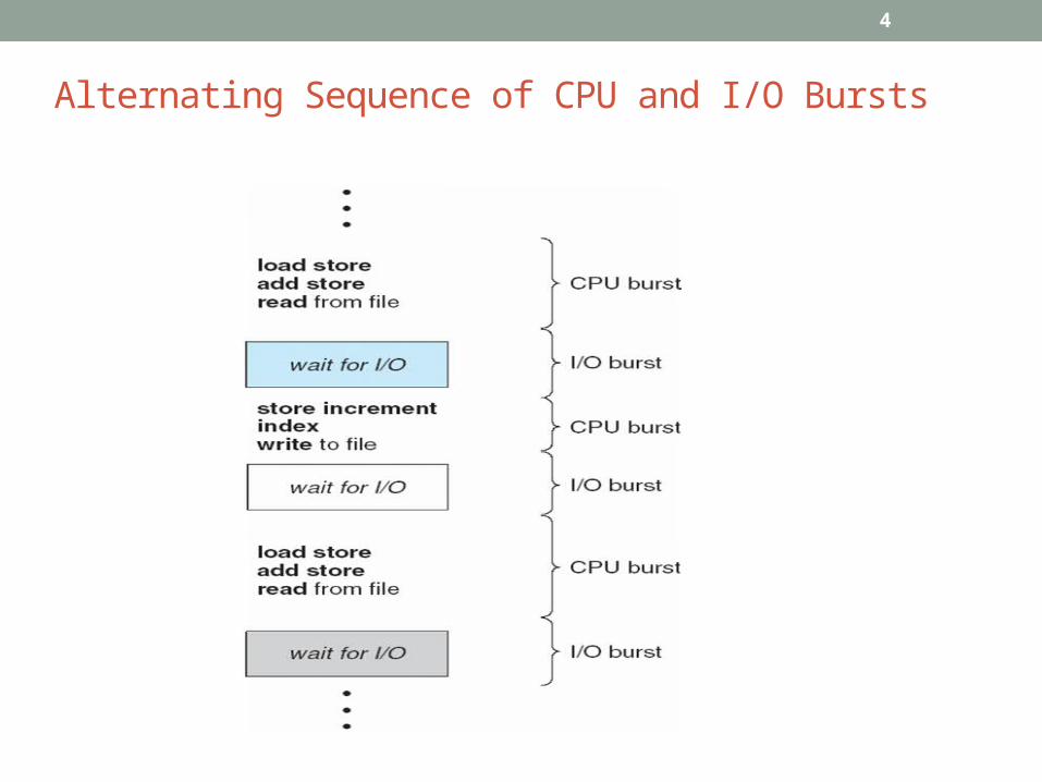
In most programs, there is alternating between I/O bursts and CPU bursts like:

Waiting time Sum of periods spent waiting in ready queue Average is across all visits to ready queue Goal: short waiting time

cin>>n>> a>> b; /* I/O wait */ for (i=1; i<=n; i++) /* CPU burst */

x = x + a*b; cout<<x; /* I/O wait */ for (i=1; i<=n; i++) /* CPU burst */

x = x + a*b; cout<<x; /* I/O wait */

3

The CPU-I/O Burst Cycle

Maximum CPU utilization obtained with multiprogramming.

CPU-I/O Burst Cycle – Process execution consists of a

cycle of CPU execution and I/O wait.

Each cycle consists of a CPU burst followed by a (usually

longer) I/O burst.

A process usually terminates on a CPU burst.

4

Alternating Sequence of CPU and I/O Bursts

5

CPU-Bound and I/O-Bound Processes

I/O Bound processes: processes that perform lots of I/O

operations. Each I/O operation is followed by a short CPU

burst to process the I/O, then more I/O happens.

CPU bound processes: processes that perform lots of

computation and do little I/O. Tend to have a few long

CPU bursts.

6

Non-preemptive vs. Preemptive Scheduling

Non-preemptive schedulingEach running process keeps the CPU until it completes or it

switches to the waiting (blocked) state.

Preemptive schedulingA running process may be also forced to release the CPU even

though it is neither completed nor blocked.

7

CPU Scheduling Criteria

1. CPU utilization – keep the CPU as busy as possible.

2. Throughput – # of processes that complete their execution per time unit.

3. Turnaround time – amount of time to execute a particular process, from submission to termination.

4. Waiting time – amount of time a process has been waiting in the ready queue.

5. Response time – amount of time it takes from when a request was submitted until the first response is produced.

6. Fairness– A scheduler makes sure that each process gets its fair share of the CPU and no process can suffer indefinite postponement.

8

CPU SchedulerSelects from among the processes in memory that are ready to

execute, and allocates the CPU to one of them.CPU scheduling decision (5 below) may take place when a process:

1) Switches from running to waiting state

2) Switches from running to ready state

3) Switches from waiting to ready

4) TerminatesScheduling under 1 and 4 is non-preemptiveAll other scheduling is preemptive

Waiting Ready

Running TerminateStart

12

3

40

5

Process life-cycle

9

DispatcherNot the same as scheduler.Dispatcher module gives control of the CPU to the process

selected by the scheduler; this involves:switching context.switching to user mode.jumping to the proper location in the user program to restart that

program.

Dispatch latency – time it takes for the dispatcher to stop one process and start another running.

10

Optimization Criteria

In CPU scheduling, the following results are sought:

Maximum CPU utilization

Maximum throughput

Minimum turnaround time

Minimum waiting time

Minimum response time

11

CPU Scheduling Algorithms

There are four well-known scheduling algorithms:

1) First Come First Served (FCFS) Scheduling

2) Shortest Job First (SJF) Scheduling

3) Priority-Based Scheduling

4) Round-Robin (RR) Scheduling

12

First Come First Served (FCFS) Scheduling

Selection function: the process that has been waiting the longest in the ready queue (hence, FCFS)

Decision mode: non-preemptivea process runs until it blocks for an I/O

13

Process Burst Time

P1 24

P2 3

P3 3

• Suppose that the processes arrive in the order: P1 , P2 , P3

The Gantt Chart for the schedule is:

• Waiting time for P1 = 0; P2 = 24; P3 = 27

• Average waiting time: (0 + 24 + 27)/3 = 17

P1 P2 P3

24 27 300

First Come First Served (FCFS) Scheduling

14

What if the processes arrive in the next order?

P2 , P3 , P1

• The Gantt chart for the schedule is:

• Waiting time for P1 = 6; P2 = 0; P3 = 3

• Average waiting time: (6 + 0 + 3)/3 = 3• Much better than previous case• Convoy effect short process behind long process

P1P3P2

63 300

First Come First Served (FCFS) Scheduling

15

FCFS and Convoy Effect

• Consider:• P1: CPU-bound (More CPU processing)

• P2, P3, P4: I/O-bound ( More I/O operations)

• P2, P3, and P4 could quickly finish their I/O request → ready queue, waiting for CPU.

• Note: I/O devices are idle then.• Then, P1 finishes its CPU burst and move to an I/O device.• P2, P3, and P4 which have short CPU bursts, finish quickly → back to I/O queue.

16

FCFS and Convoy Effect (Cont’d)

• Note: CPU is idle then.

• P1 moves then back to ready queue is gets allocated

CPU time.

• Again P2, P3, and P4 wait behind P1 when they request

CPU time.

One Reason behind this problem is that, FCFS is non-

preemptive.P1 keeps the CPU as long as it needs

17

FCFS: Critique

• Favors CPU-bound processes• A CPU-bound process monopolizes the processor• I/O-bound processes have to wait until completion of CPU-bound

process

• I/O-bound processes may have to wait even after their I/Os are completed (poor device utilization)

• Better I/O device utilization could be achieved if I/O bound processes had higher priority

18

• Selection function: the process with the shortest expected CPU burst time• I/O-bound processes will be selected first

• Decision mode: non-preemptive• The required processing time, i.e., the CPU burst time,

must be estimated for each process

Shortest Job First (SJF) Scheduling

19

Shortest Job First (SJF) Scheduling

• Two schemes: • Non-preemptive – once CPU given to the process it cannot be

preempted until completes its CPU burst• Preemptive – if a new process arrives with CPU burst length less

than remaining time of currently executing process, preempt the current process. This scheme is know as the Shortest Remaining Time First (SRTF)

• SJF algorithm is optimal • Gives a schedule with least average waiting time among all possible

scheduling algorithms• SJF is proven optimal only when all jobs are available

simultaneously.

20

• Assume all processes arrive at the same time:

P1 , P2 , P3 , P4

• Non-preemptive scheduling

Gantt chart

• Average waiting time: (3+16+9+0)/4=7 ms

P2P1P4

93 240

P3

16

PID Burst

P1 6

P2 8

P3 7

P4 3

Non-Preemptive SJF (Example-1)

21

Process Arrival Time Burst Time

P1 0.0 7

P2 2.0 4

P3 4.0 1

P4 5.0 4

• SJF (non-preemptive)

• Average waiting time = (0 + 6 + 3 + 7)/4 = 4

Non-Preemptive SJF (Example-2)

P1 P3 P2

73 160

P4

8 12

22

Preemptive SJF or Shortest Remaining Time First (SRTF)-Example

Process Arrival Time Burst Time

P1 0.0 7

P2 2.0 4

P3 4.0 1

P4 5.0 4

• SJF (preemptive)

• Average waiting time = (9 + 1 + 0 +2)/4 = 3

P1 P3P2

42 110

P4

5 7

P2 P1

16

23

SJF: Critique

Possibility of starvation for longer processes.

Lack of preemption is not suitable in a time sharing

environment.

SJF implicitly incorporates priorities.

• Shortest jobs are given preferences

• CPU bound process have lower priority, but a process doing no

I/O could still monopolize the CPU if it is the first to enter the

system

24

Priority-Based Scheduling

• A priority number (integer) is associated with each process• The CPU is allocated to the process with the highest priority

(smallest integer highest priority)• Again two types

• Preemptive• nonpreemptive

• SJF is a priority scheduling algorithm where priority is the (inverse of) predicted next CPU burst time

• Problem Starvation low priority processes may never execute• Solution Aging as time progresses increase the priority of a

lower priority process that is not receiving CPU time.

Example with four priority classes

25

Example of Priority-Based Scheduling

Process Burst Time Priority

P1 10 3

P2 1 1

P3 2 4

P4 1 5

P5 5 2

• Gantt Chart

• Average waiting time =(0+1+6+16+18)/5=8.2 msec

P2 P3P5

1 180 16

P4

196

P1

26

Selection function: same as FCFS

Decision mode: preemptive

a process is allowed to run until the time slice period (quantum,

typically from 10 to 100 ms) has expired

a clock interrupt occurs and the running process is put on the

ready queue

Round-Robin (RR) Scheduling

27

Round-Robin (RR) Scheduling (Cont’d)• Each process gets a small unit of CPU time (time quantum), usually

10-100 milliseconds.

• After this time has elapsed, the process is preempted and added to the end of the ready queue.

• If there are n processes in the ready queue and the time quantum is q, then each process gets 1/n of the CPU time in chunks of at most q time units at once. No process waits more than (n-1)q time units.

• Performance• q large FCFS• q small Too much context switching. q must be large compared

to context switch time, otherwise overhead is too high

28

Choosing RR Time Quantum

• Quantum must be substantially larger than the time

required to handle the clock interrupt and dispatching

• Quantum should be larger then the typical interaction

• but not much larger, to avoid penalizing I/O bound processes

29

Choosing RR Time Quantum (Cont’d)

30

Choosing RR Time Quantum (Cont’d)

The effect of quantum size on context-switching time must

be carefully considered.

Larger the time quantum, larger the response time.

Smaller the time quantum, more the number of context

switches.

Modern systems use quanta from 10 to 100 msec with

context switch taking < 10 msec

31

Choosing RR Time Quantum (Cont’d)

32

Turnaround Time Varies With The Time Quantum

80% of CPU bursts should be shorter than q

33

Example of RR with Time Quantum = 20

Process Burst Time

P1 53

P2 17

P3 68

P4 24

• The Gantt chart is:

• Typically, higher average turnaround than SJF, but better response time

P1 P2 P3 P4 P1 P3 P4 P1 P3 P3

0 20 37 57 77 97 117 121 134 154 162

34

• Assume processes arrive in this order:

P1 , P2 , P3 • Preemptive scheduling • Time quantum: 4 ms

Gantt chart

• P1 uses a full time quantum; P2, P3 use only a part of a quantum

• P1 waits 0+6=6; P2 waits 4; P3 waits 7 • Average waiting time: (6+4+7)/3=5.66 ms

PID Burst

P1 24

P2 3

P3 3

P1 P2 P3 P1 P1 P1 P1 P1

0 4 7 10 14 18 22 26 30

Example of RR with Time Quantum = 4

35

Round Robin: Critique

• Still favors CPU-bound processes

• An I/O bound process uses the CPU for a time less than the time

quantum before it is blocked waiting for an I/O

• A CPU-bound process runs for all its time slice and is put back into

the ready queue

• May unfairly get in front of blocked processes