chapter 5 two-dimensional plots - islamic university of...
TRANSCRIPT

Computer Programming
ECIV 2303
Instructor: Dr. Talal Skaik
Islamic University of Gaza
Faculty of Engineering
Chapter 5
Two-Dimensional Plots
1Dr. Talal Skaik 2018

Introduction
Plots are a very useful tool for presenting information.
MATLAB has many commands that can be used for creating different types of plots.
These include standard plots with linear axes, plots with logarithmic bar and stairs plots,
polar plots, three-dimensional contour surface and mesh plots, and many more.
The plots can be formatted to have a desired appearance.
The line type (solid, dashed, etc.), color, and thickness can be prescribed, line markers
and grid lines can be added, as can titles and text comments.
Several graphs can be created in the same plot, and several plots can be placed on the
same page.
2Dr. Talal Skaik 2018

Introduction
3Dr. Talal Skaik 2018

5.1 THE plot COMMAND
4Dr. Talal Skaik 2018
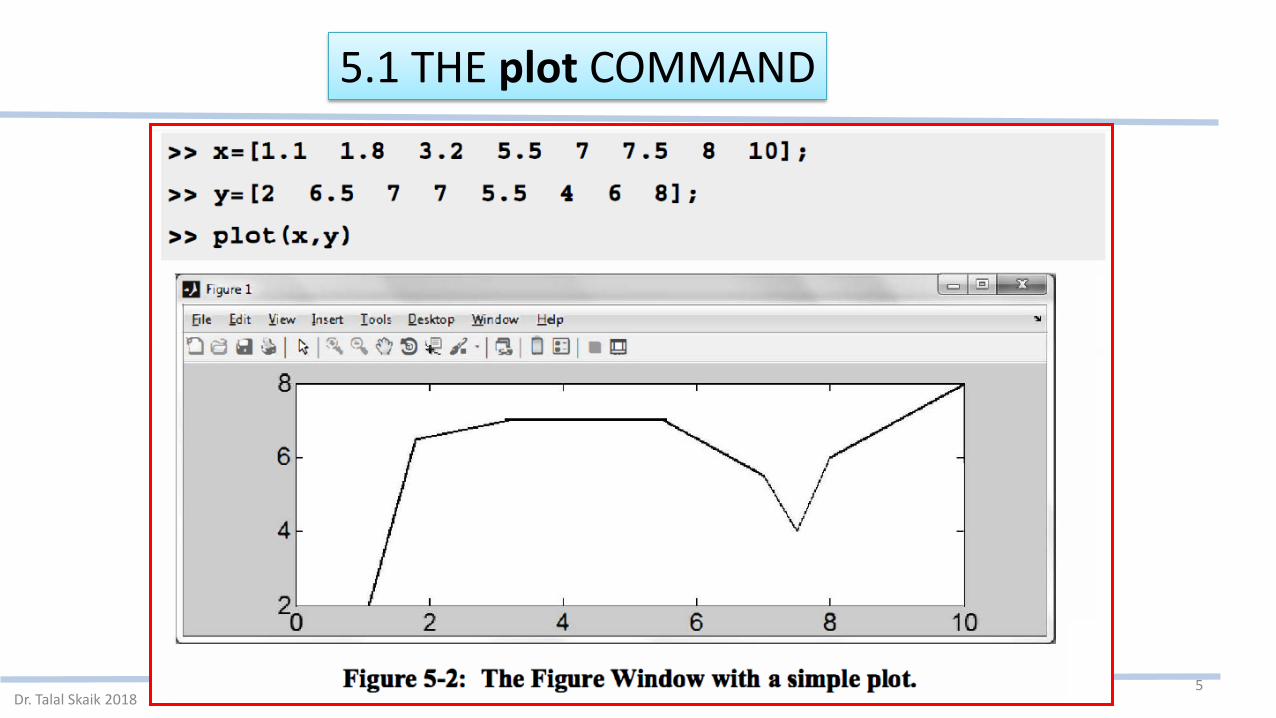
The plot command is used to create two-dimensional plots. The simplest form of the
command is:
The arguments x and y are each a vector (one-dimensional array).
The two vectors must have the same number of elements.
When the plot command is executed, a figure is created in the Figure Window.
The figure has a single curve with the x values on the horizontal axis and the y values on
the vertical axis.
If only one vector is entered as an input argument in the plot command (for example:
plot (y)) then the figure will show a plot of the values of the elements of the vector ( y(l),
y(2), y(3), ... ) versus the element number ( 1, 2, 3, ... ).
5.1 THE plot COMMAND
5Dr. Talal Skaik 2018

5.1 THE plot COMMAND
6Dr. Talal Skaik 2018
The plot command has additional, optional arguments that can be used to specify the color and
style of the line and the color and type of markers, if any are desired.

5.1 THE plot COMMAND
7
Line Specifiers: optional, can be used to define the style and color of the line and the type of markers.
Dr. Talal Skaik 2018

5.1 THE plot COMMAND
8Dr. Talal Skaik 2018

5.1 THE plot COMMAND
9
Notes about using the specifiers:• The specifiers are typed inside the plot command as strings.
• Within the string the specifiers can be typed in any order.
• The specifiers are optional. This means that none, one, two, or all three types can be included
in a command.
Dr. Talal Skaik 2018
5.1 THE plot COMMAND
10
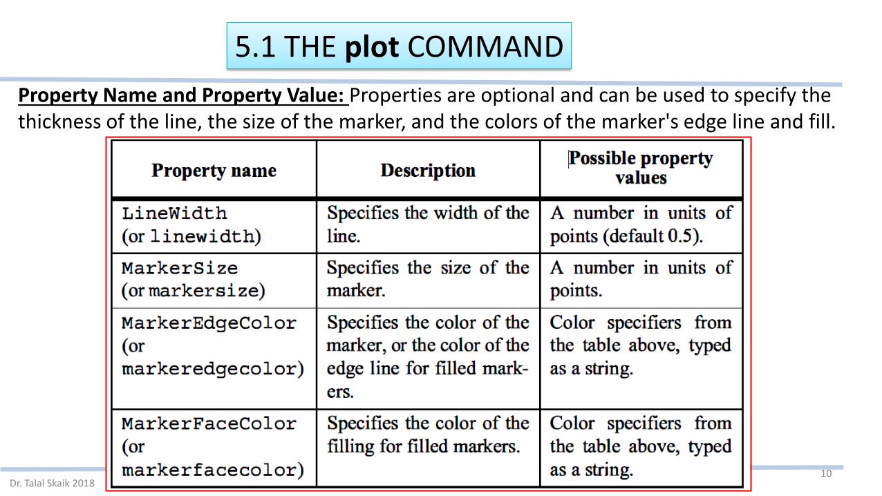
Property Name and Property Value: Properties are optional and can be used to specify the thickness of the line, the size of the marker, and the colors of the marker's edge line and fill.
Dr. Talal Skaik 2018
5.1 THE plot COMMAND
11
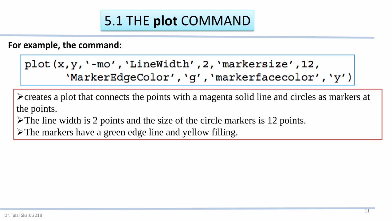
For example, the command:
Dr. Talal Skaik 2018
creates a plot that connects the points with a magenta solid line and circles as markers at
the points.
The line width is 2 points and the size of the circle markers is 12 points.
The markers have a green edge line and yellow filling.

5.1 THE plot COMMAND
12Dr. Talal Skaik 2018
A note about line specifiers and properties:
The three line specifiers, which indicate the style and color of the line, and the type of the marker
can also be assigned with a PropertyName argument followed by a PropertyValue argument.

5.1.1 Plot of Given Data
13Dr. Talal Skaik 2018
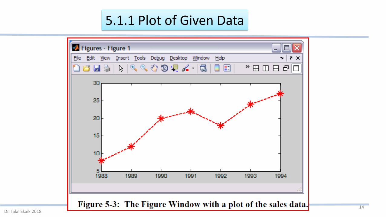
5.1.1 Plot of Given Data
14Dr. Talal Skaik 2018
5.1.2 Plot of a Function
15Dr. Talal Skaik 2018
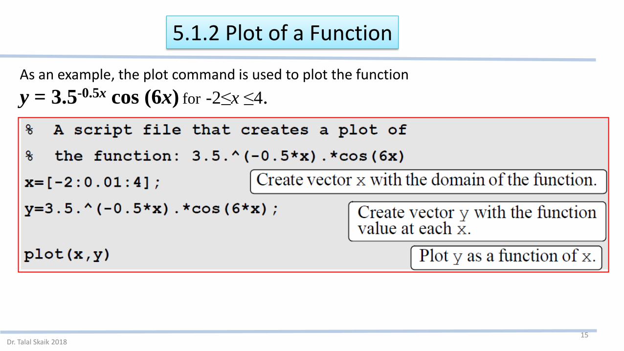
As an example, the plot command is used to plot the function
y = 3.5-0.5x cos (6x) for -2≤x ≤4.

5.1.2 Plot of a Function
16Dr. Talal Skaik 2018

5.1.2 Plot of a Function
17Dr. Talal Skaik 2018
In the last example a small spacing of 0.01 produced the plot of the function.
If larger spacing is used, for example, 0.3, the plot gives a distorted picture of the function.

5.2 THE fplot COMMAND
18Dr. Talal Skaik 2018
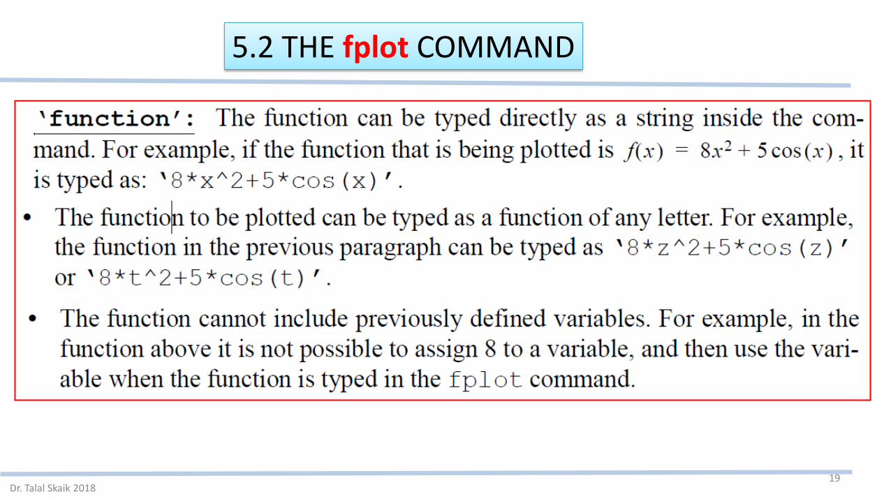
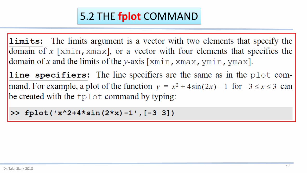
The fplot command plots a function with the form y = f(x) between specified limits. The command has the form:
5.2 THE fplot COMMAND
19Dr. Talal Skaik 2018
5.2 THE fplot COMMAND
20Dr. Talal Skaik 2018

5.2 THE fplot COMMAND
21Dr. Talal Skaik 2018
5.3 PLOTTING MULTIPLE GRAPHS IN THE SAME PLOT
22Dr. Talal Skaik 2018
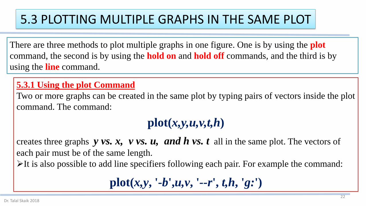
There are three methods to plot multiple graphs in one figure. One is by using the plot
command, the second is by using the hold on and hold off commands, and the third is by
using the line command.
5.3.1 Using the plot Command
Two or more graphs can be created in the same plot by typing pairs of vectors inside the plot
command. The command:
plot(x,y,u,v,t,h)
creates three graphs y vs. x, v vs. u, and h vs. t all in the same plot. The vectors of
each pair must be of the same length.
It is also possible to add line specifiers following each pair. For example the command:
plot(x,y, '-b',u,v, '--r', t,h, 'g:')

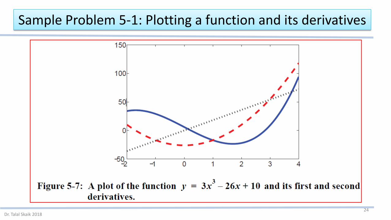
Sample Problem 5-1: Plotting a function and its derivatives
23Dr. Talal Skaik 2018
Plot the function y = 3x3- 26x + 10, and its first and second derivatives, for -2 ≤ x ≤ 4, all in the same plot.SolutionThe first derivative of the function is: y’ = 9x2- 26.The second derivative of the function is: y” = 18x.
Sample Problem 5-1: Plotting a function and its derivatives
24Dr. Talal Skaik 2018

5.3.2 Using the hold on and hold off Commands
25Dr. Talal Skaik 2018
To plot several graphs using the hold on and hold off commands, one graph is plotted
first with the plot command. Then the hold on command is typed.
This keeps the Figure Window with the first plot open including the axis properties and
formatting.
Additional graphs can be added with plot commands that are typed next. Each plot
command creates a graph that is added to that figure.
The hold off command stops this process. It returns MATLAB to the default mode, in
which the plot command erases the previous plot and resets the axis properties.

5.3.2 Using the hold on and hold off Commands
26Dr. Talal Skaik 2018

5.3.3 Using the line Command
27Dr. Talal Skaik 2018
With the line command additional graphs (lines) can be added to a plot that already exists.
The properties are optional, and if none are entered MATLAB uses default properties and
values. For example, the command:
line(x,y, 'linestyle', '--','color', 'r', 'marker', 'o')
will add a dashed red line with circular markers to a plot that already exists.

5.3.3 Using the line Command
28Dr. Talal Skaik 2018
The major difference between the plot and line commands is that the plot command starts
a new plot every time it is executed, while the line command adds lines to a plot that already
exists.
To make a plot that has several graphs, a plot command is typed first and then line
commands are typed for additional graphs. (If a line command is entered before a plot
command, an error message is displayed.)

5.4 FORMATTING A PLOT
29Dr. Talal Skaik 2018
5.4.1 Formatting a Plot Using Commands
The xlabel and ylabel commands:
The title command:
The text command:
The text command places the text in the figure such that the first character is positioned at the
point with the coordinates x, y (according to the axes of the figure).
The gtext command places the text at a position specified by the user. When the command is
executed, the Figure Window opens and the user specifies the position with the mouse.

5.4 FORMATTING A PLOT
30Dr. Talal Skaik 2018
The legend command:

5.4 FORMATTING A PLOT
31Dr. Talal Skaik 2018
Formatting the text within the xlabel, ylabel, title, text and legend commands:
The formatting can be used to define the font, size, position (superscript, subscript), style
(italic, bold, etc.), and color of the characters, the color of the background, and many other
details of the display.
The formatting can be done either by adding modifiers inside the string, or by adding to
the command optional PrapertyName and PrapertyValue arguments following the string.

5.4 FORMATTING A PLOT
32Dr. Talal Skaik 2018
Formatting the text within the xlabel, ylabel, title, text and legend commands:
Subscript and superscript:
A single character can be displayed as a subscript or a superscript by typing_ (the
underscore character) or ^ in front of the character, respectively.
Several consecutive characters can be displayed as a subscript or a superscript by typing
the characters inside braces { } following the_ or the ^.

5.4 FORMATTING A PLOT
33Dr. Talal Skaik 2018
Formatting the text within the xlabel, ylabel, title, text and legend commands:
Greek characters:

5.4 FORMATTING A PLOT
34Dr. Talal Skaik 2018
Formatting the text within thexlabel, ylabel, title, text andlegend commands:
Formatting of the text can also be done
by adding optional PropertyName and
PropertyValue arguments following the
string inside the command.

5.4 FORMATTING A PLOT
35Dr. Talal Skaik 2018
The axis command:
The grid command:

5.4 FORMATTING A PLOT
36Dr. Talal Skaik 2018
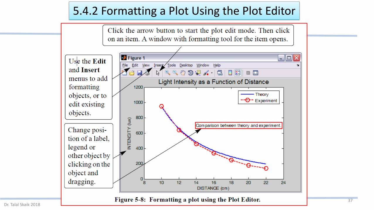
5.4.2 Formatting a Plot Using the Plot Editor
37Dr. Talal Skaik 2018

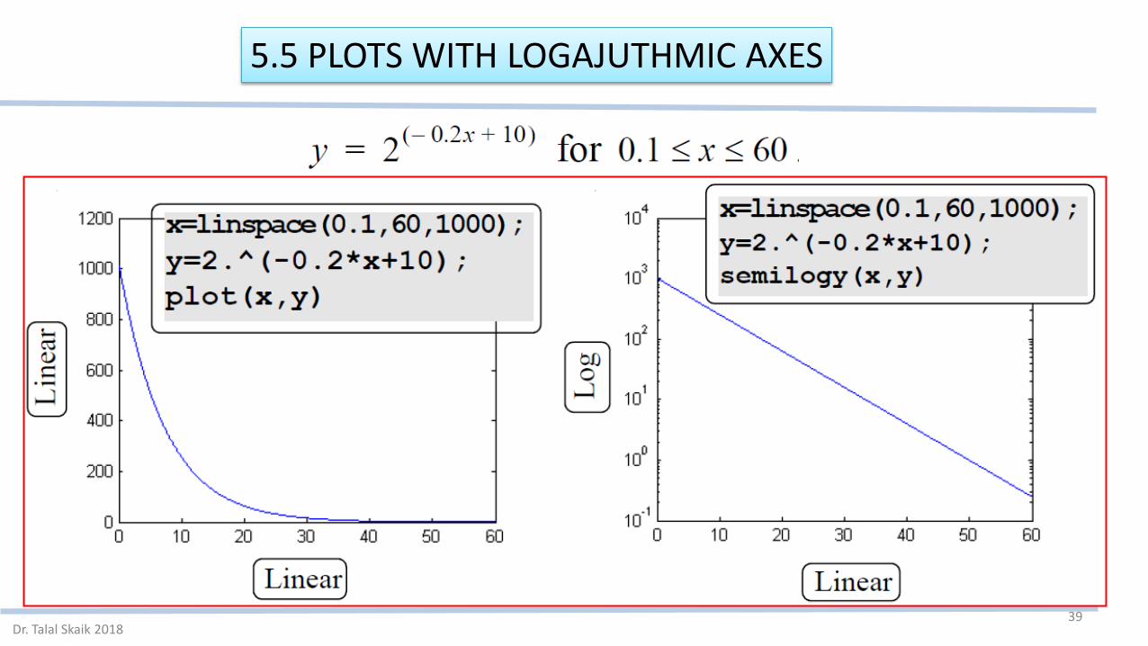
5.5 PLOTS WITH LOGAJUTHMIC AXES
38Dr. Talal Skaik 2018
Line specifiers and Property Name and Property Value arguments can be added to the commands (optional) just as in the plot command
5.5 PLOTS WITH LOGAJUTHMIC AXES
39Dr. Talal Skaik 2018

5.5 PLOTS WITH LOGAJUTHMIC AXES
40Dr. Talal Skaik 2018

5.6 PLOTS WITH ERROR BARS
41Dr. Talal Skaik 2018
An error bar is typically a short vertical line that is attached to a data point in a plot.
It shows the magnitude of the error that is associated with the value that is displayed by the
data point.

5.6 PLOTS WITH ERROR BARS
42Dr. Talal Skaik 2018
The lengths of the three vectors x, y, and e must be the same.The length of the error bar is twice the value of e. At each point the error bar extends from y(i)-e(i) to y(i)+e(i).
Symmetric error bar: the error bar extends the same length above and below the data point

5.6 PLOTS WITH ERROR BARS
Dr. Talal Skaik 201843

5.6 PLOTS WITH ERROR BARS
Dr. Talal Skaik 201844
Non-symmetric error bars:
The lengths of the four vectors x, y, d, and u must be the same.At each point the error bar extends from y(i)-d(i) to y(i)+u(i).

5. 7 PLOTS WITH SPECIAL GRAPHICS
Dr. Talal Skaik 201845
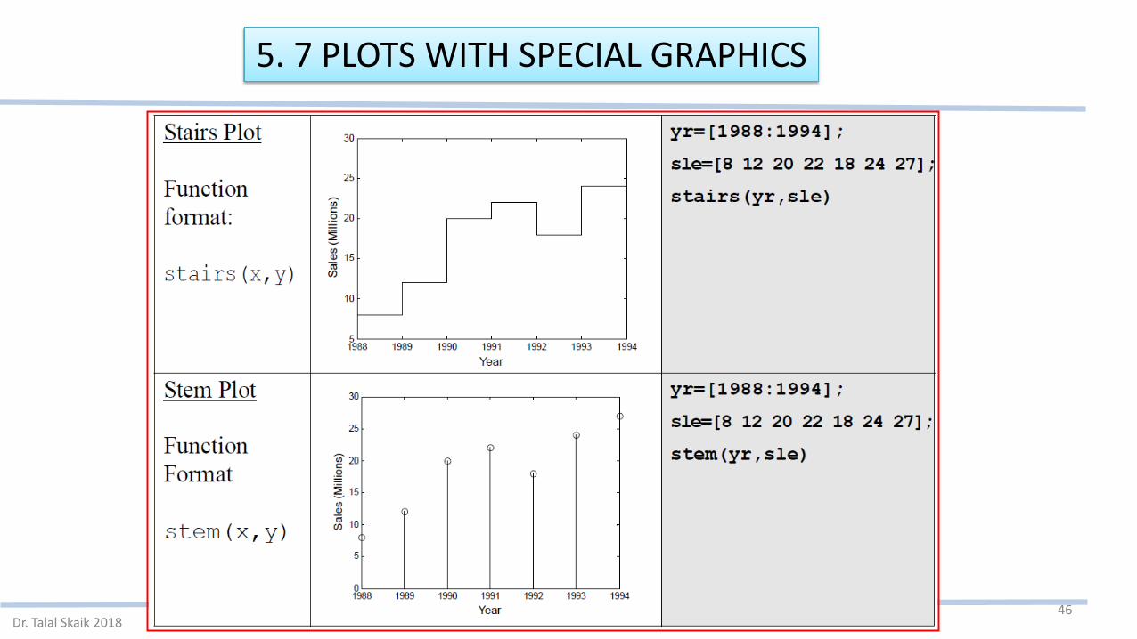
5. 7 PLOTS WITH SPECIAL GRAPHICS
Dr. Talal Skaik 201846

5. 7 PLOTS WITH SPECIAL GRAPHICS
Dr. Talal Skaik 201847
5.8 HISTOGRAMS
Dr. Talal Skaik 201848
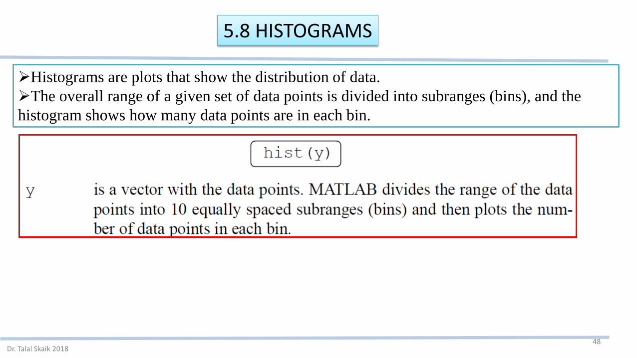
Histograms are plots that show the distribution of data.
The overall range of a given set of data points is divided into subranges (bins), and the
histogram shows how many data points are in each bin.

5.8 HISTOGRAMS
Dr. Talal Skaik 201849
The following data points are the daily maximum temperature (in F) during the month of April: 58
73 73 53 50 48 56 73 73 66 69 63 74 82 84 91 93 89 91 80 59 69 56 64 63 66 64 74 63 69

5.8 HISTOGRAMS
Dr. Talal Skaik 201850
The smallest value in the data set is 48 and
the largest is 93, which means that the range is
45 and the width of each bin is 4.5.
The range of the first bin is from 48 to 52.5
and contains two points. The range of the
second bin is from 52.5 to 57 and contains
three points, and so on.
Two of the bins (75 to 79.5 and 84 to 88.5)
do not contain any points.

5.8 HISTOGRAMS
Dr. Talal Skaik 201851
The number of bins can be defined to be different than 10. This can be done either by
specifying the number of bins, or by specifying the center point of each bin:

5.8 HISTOGRAMS
Dr. Talal Skaik 201852

5.8 HISTOGRAMS
Dr. Talal Skaik 201853

5.8 HISTOGRAMS
Dr. Talal Skaik 201854
The vector n shows that the first bin has two data points, the second bin has three data points, and so on.
Fig.5-11

5.8 HISTOGRAMS
Dr. Talal Skaik 201855

5.9 POLAR PLOTS
Dr. Talal Skaik 201856
Polar coordinates, in which the position of a point in a plane is defined
by the angle θ and the radius (distance) to the point, are frequently used
in the solution of science and engineering problems.

5.9 POLAR PLOTS
Dr. Talal Skaik 201857
To plot a function r = f(θ) in a certain domain, a vector for values of θ is created first, and then a
vector r with the corresponding values of is created using element-by-element calculations.
5.10 PUTTING MULTIPLE PLOTS ON THE SAME PAGE
Dr. Talal Skaik 201858
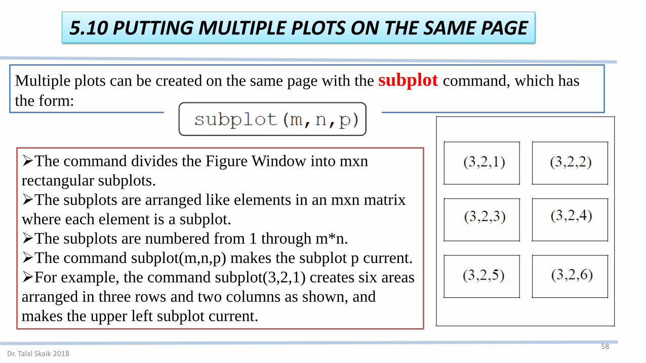
Multiple plots can be created on the same page with the subplot command, which has
the form:
The command divides the Figure Window into mxn
rectangular subplots.
The subplots are arranged like elements in an mxn matrix
where each element is a subplot.
The subplots are numbered from 1 through m*n.
The command subplot(m,n,p) makes the subplot p current.
For example, the command subplot(3,2,1) creates six areas
arranged in three rows and two columns as shown, and
makes the upper left subplot current.