chapter 5: process scheduling - national taiwan...
TRANSCRIPT
Silberschatz, Galvin and Gagne © 2013Operating System Concepts – 9th Edition
Chapter 5: Process
Scheduling

6.2 Silberschatz, Galvin and Gagne © 2013Operating System Concepts – 9th Edition
Chapter 5: Process Scheduling
Basic Concepts
Scheduling Criteria
Scheduling Algorithms
Thread Scheduling
Multiple-Processor Scheduling
Real-Time CPU Scheduling
Operating Systems Examples
Algorithm Evaluation

6.3 Silberschatz, Galvin and Gagne © 2013Operating System Concepts – 9th Edition
Objectives
To introduce CPU scheduling, which is the basis for
multiprogrammed operating systems
To describe various CPU-scheduling algorithms
To discuss evaluation criteria for selecting a CPU-
scheduling algorithm for a particular system
To examine the scheduling algorithms of several operating
systems
6.4 Silberschatz, Galvin and Gagne © 2013Operating System Concepts – 9th Edition
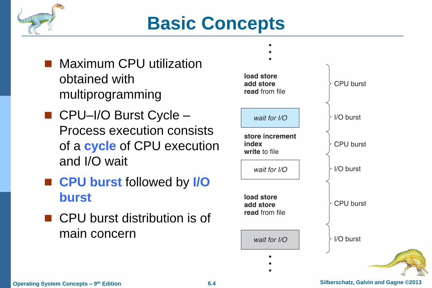
Basic Concepts
Maximum CPU utilization
obtained with
multiprogramming
CPU–I/O Burst Cycle –
Process execution consists
of a cycle of CPU execution
and I/O wait
CPU burst followed by I/O
burst
CPU burst distribution is of
main concern
6.5 Silberschatz, Galvin and Gagne © 2013Operating System Concepts – 9th Edition
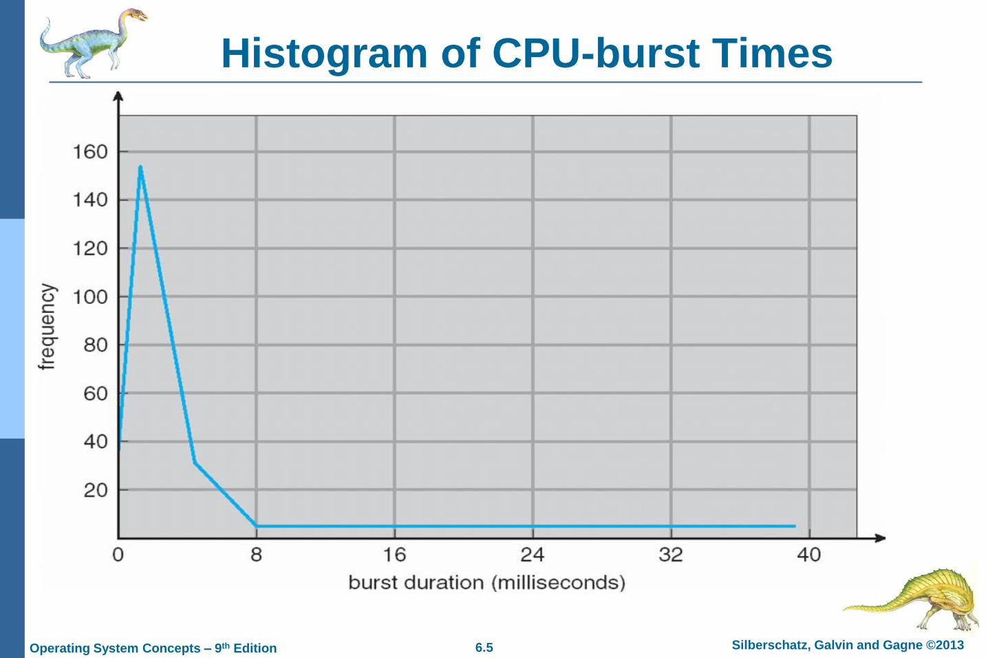
Histogram of CPU-burst Times
6.6 Silberschatz, Galvin and Gagne © 2013Operating System Concepts – 9th Edition
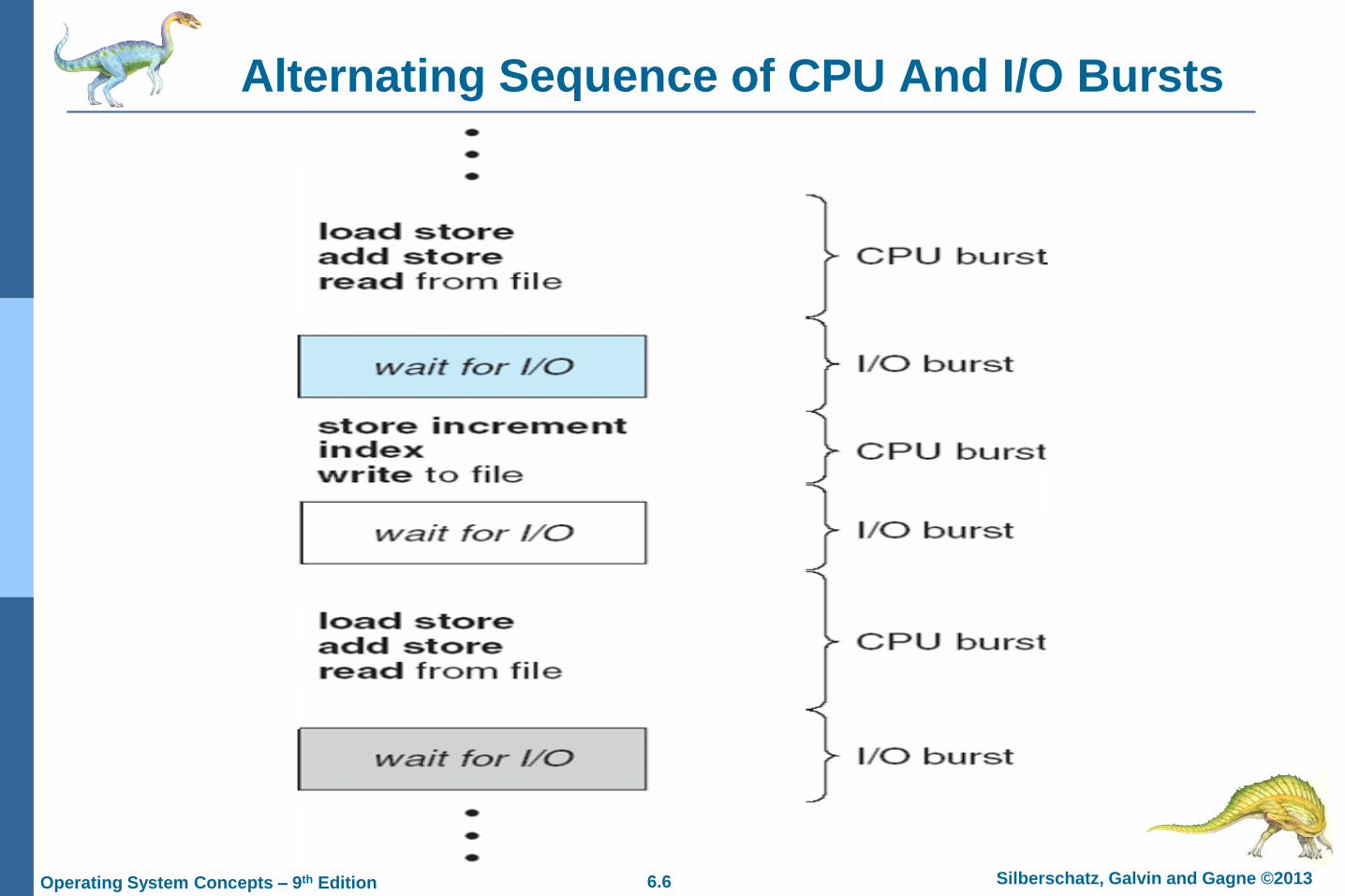
Alternating Sequence of CPU And I/O Bursts
6.7 Silberschatz, Galvin and Gagne © 2013Operating System Concepts – 9th Edition
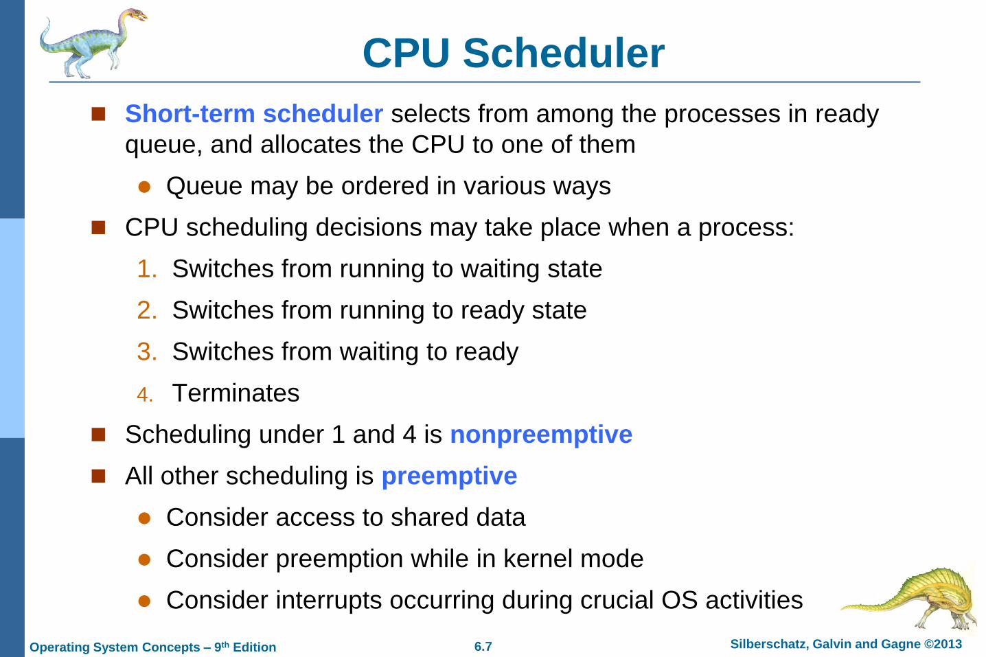
CPU Scheduler
Short-term scheduler selects from among the processes in ready
queue, and allocates the CPU to one of them
Queue may be ordered in various ways
CPU scheduling decisions may take place when a process:
1. Switches from running to waiting state
2. Switches from running to ready state
3. Switches from waiting to ready
4. Terminates
Scheduling under 1 and 4 is nonpreemptive
All other scheduling is preemptive
Consider access to shared data
Consider preemption while in kernel mode
Consider interrupts occurring during crucial OS activities
6.8 Silberschatz, Galvin and Gagne © 2013Operating System Concepts – 9th Edition
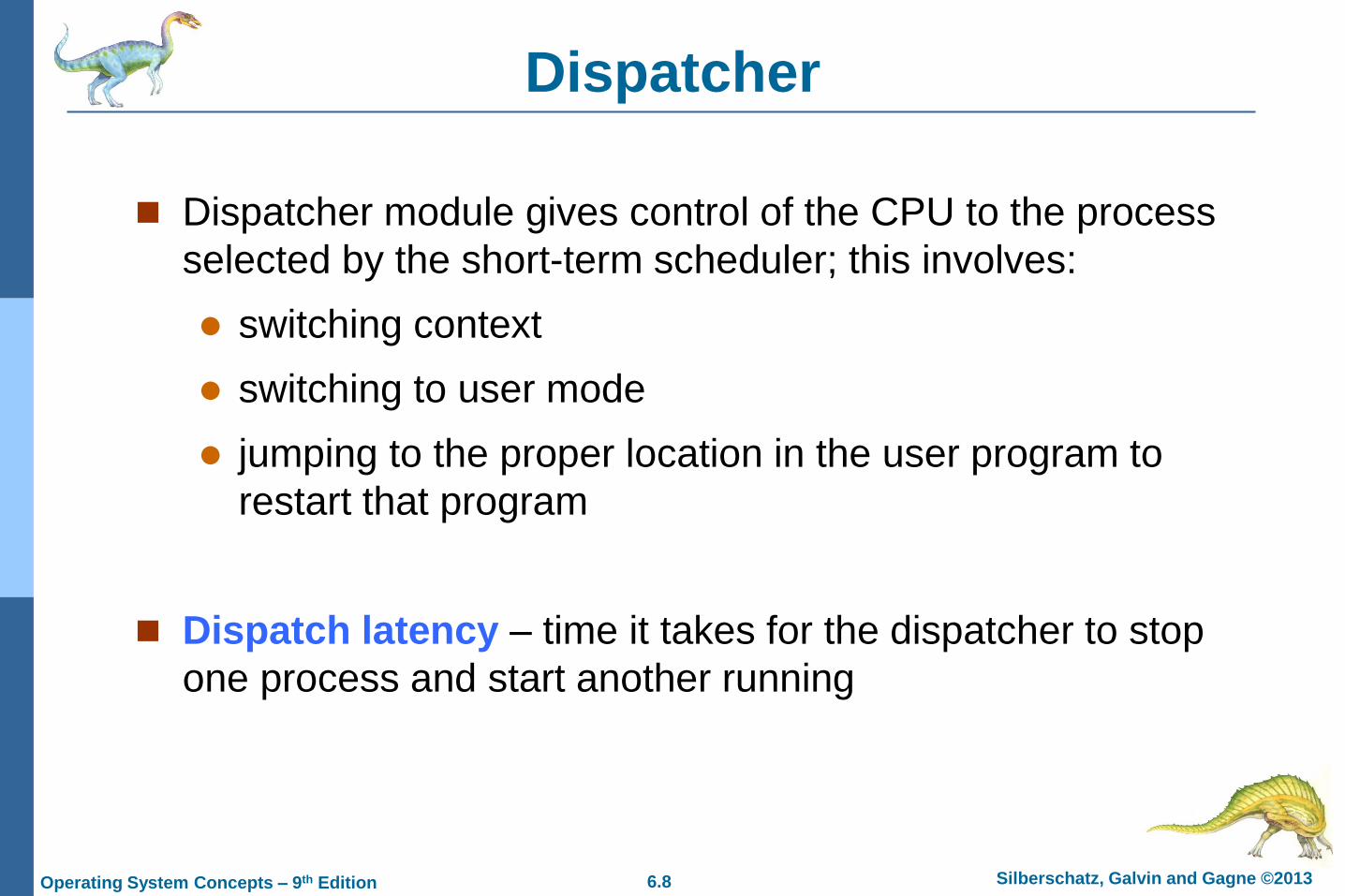
Dispatcher
Dispatcher module gives control of the CPU to the process
selected by the short-term scheduler; this involves:
switching context
switching to user mode
jumping to the proper location in the user program to
restart that program
Dispatch latency – time it takes for the dispatcher to stop
one process and start another running
6.9 Silberschatz, Galvin and Gagne © 2013Operating System Concepts – 9th Edition
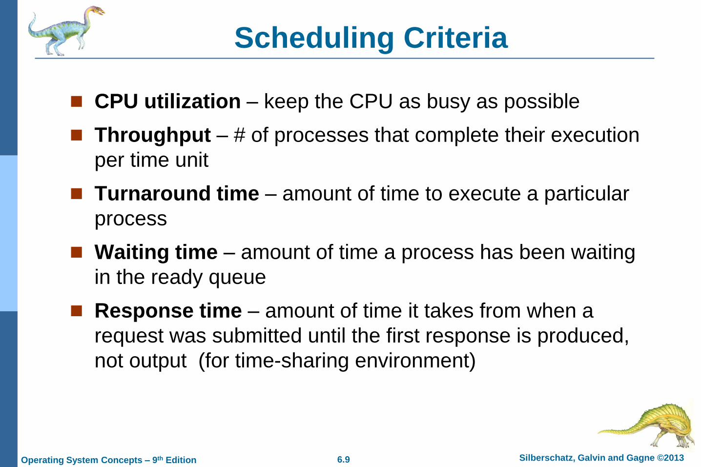
Scheduling Criteria
CPU utilization – keep the CPU as busy as possible
Throughput – # of processes that complete their execution
per time unit
Turnaround time – amount of time to execute a particular
process
Waiting time – amount of time a process has been waiting
in the ready queue
Response time – amount of time it takes from when a
request was submitted until the first response is produced,
not output (for time-sharing environment)

6.10 Silberschatz, Galvin and Gagne © 2013Operating System Concepts – 9th Edition
Scheduling Algorithm Optimization Criteria
Max CPU utilization
Max throughput
Min turnaround time
Min waiting time
Min response time
6.11 Silberschatz, Galvin and Gagne © 2013Operating System Concepts – 9th Edition
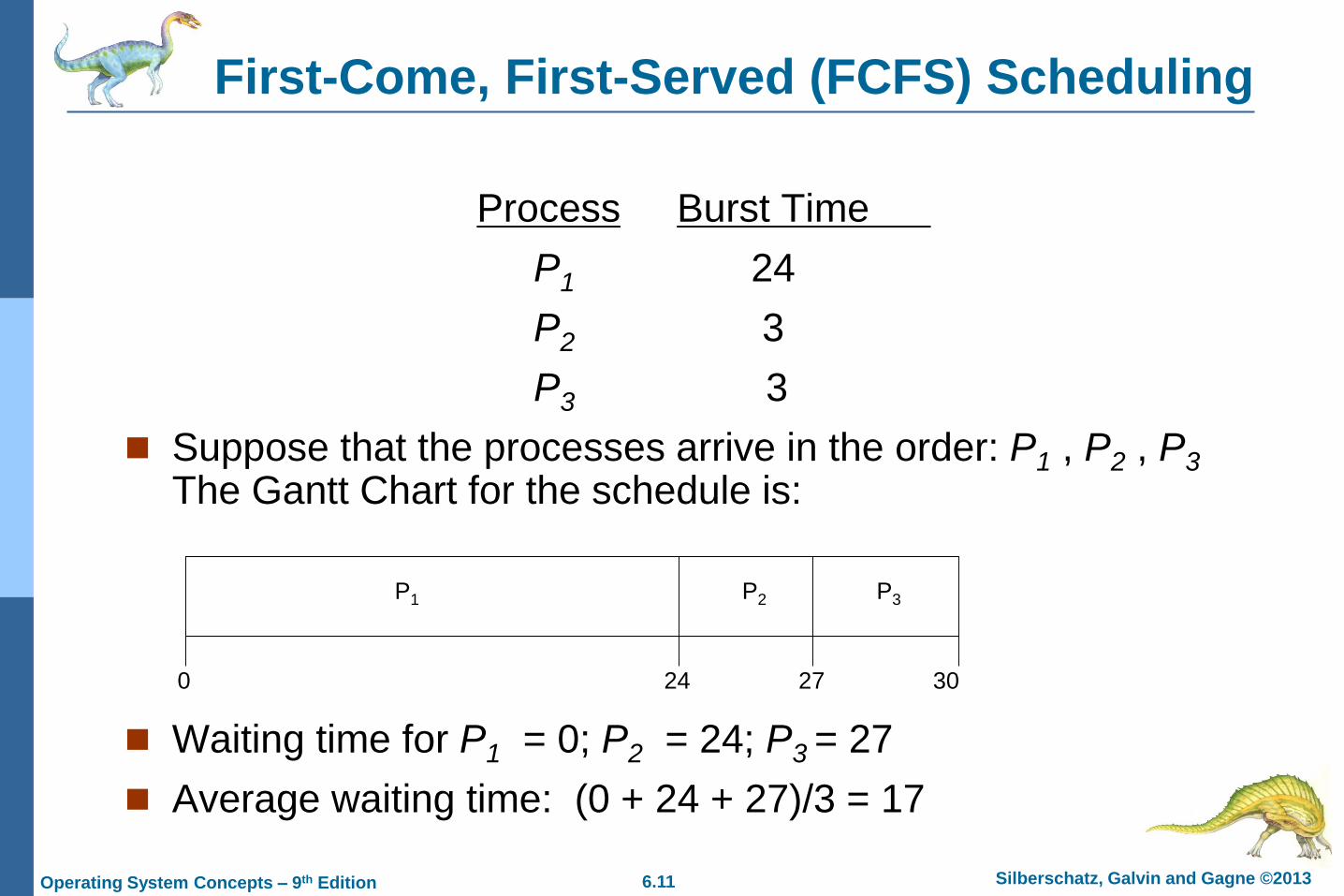
First-Come, First-Served (FCFS) Scheduling
Process Burst Time
P1 24
P2 3
P3 3
Suppose that the processes arrive in the order: P1 , P2 , P3
The Gantt Chart for the schedule is:
Waiting time for P1 = 0; P2 = 24; P3 = 27
Average waiting time: (0 + 24 + 27)/3 = 17
P1 P2 P3
24 27 300
6.12 Silberschatz, Galvin and Gagne © 2013Operating System Concepts – 9th Edition
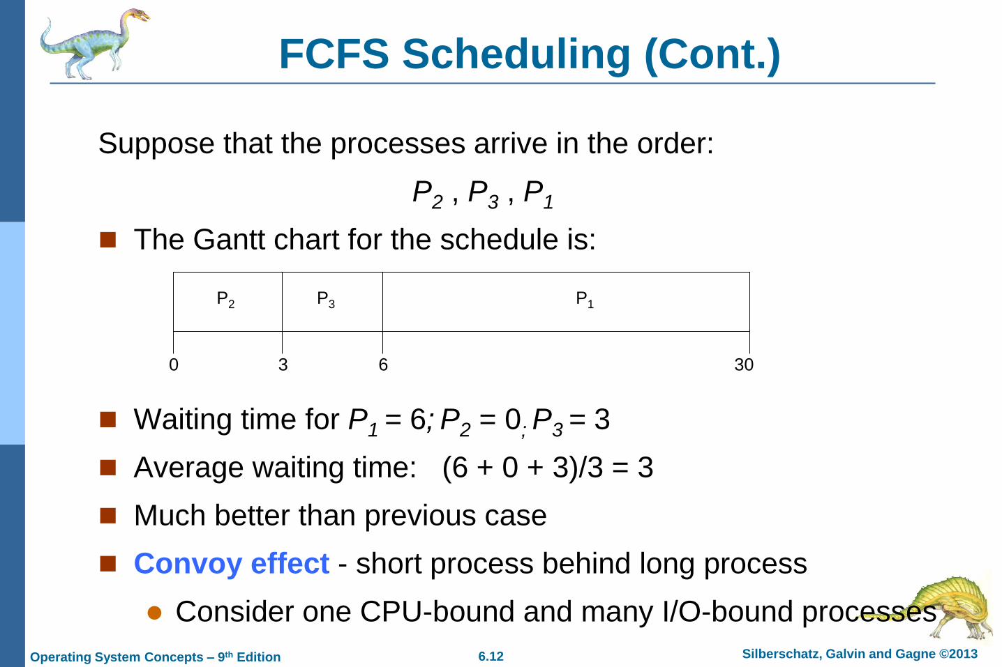
FCFS Scheduling (Cont.)
Suppose that the processes arrive in the order:
P2 , P3 , P1
The Gantt chart for the schedule is:
Waiting time for P1 = 6; P2 = 0; P3 = 3
Average waiting time: (6 + 0 + 3)/3 = 3
Much better than previous case
Convoy effect - short process behind long process
Consider one CPU-bound and many I/O-bound processes
P1P3P2
63 300
6.13 Silberschatz, Galvin and Gagne © 2013Operating System Concepts – 9th Edition
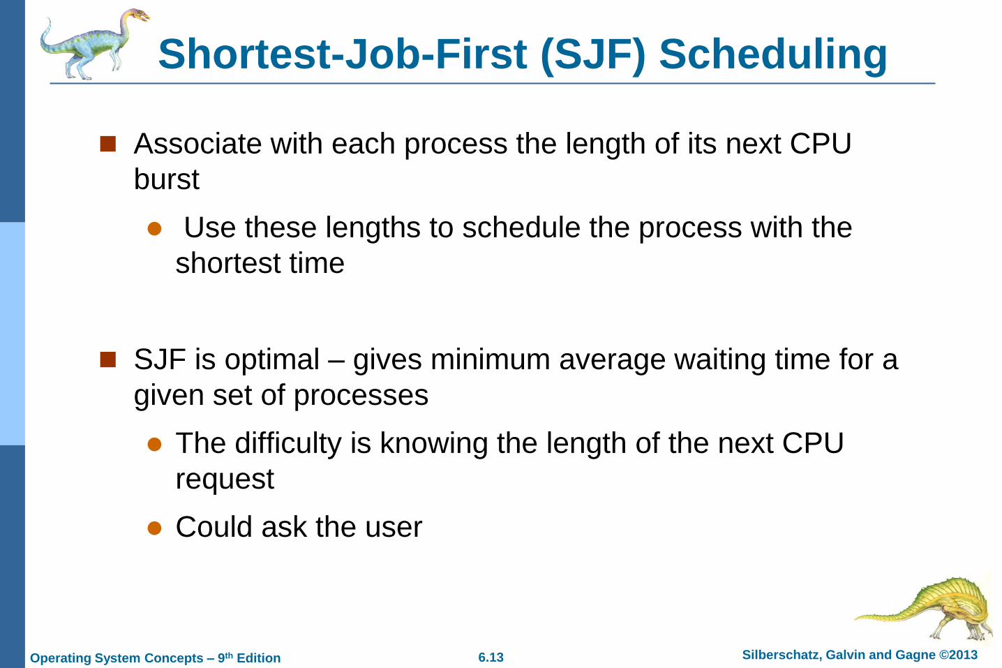
Shortest-Job-First (SJF) Scheduling
Associate with each process the length of its next CPU
burst
Use these lengths to schedule the process with the
shortest time
SJF is optimal – gives minimum average waiting time for a
given set of processes
The difficulty is knowing the length of the next CPU
request
Could ask the user
6.14 Silberschatz, Galvin and Gagne © 2013Operating System Concepts – 9th Edition
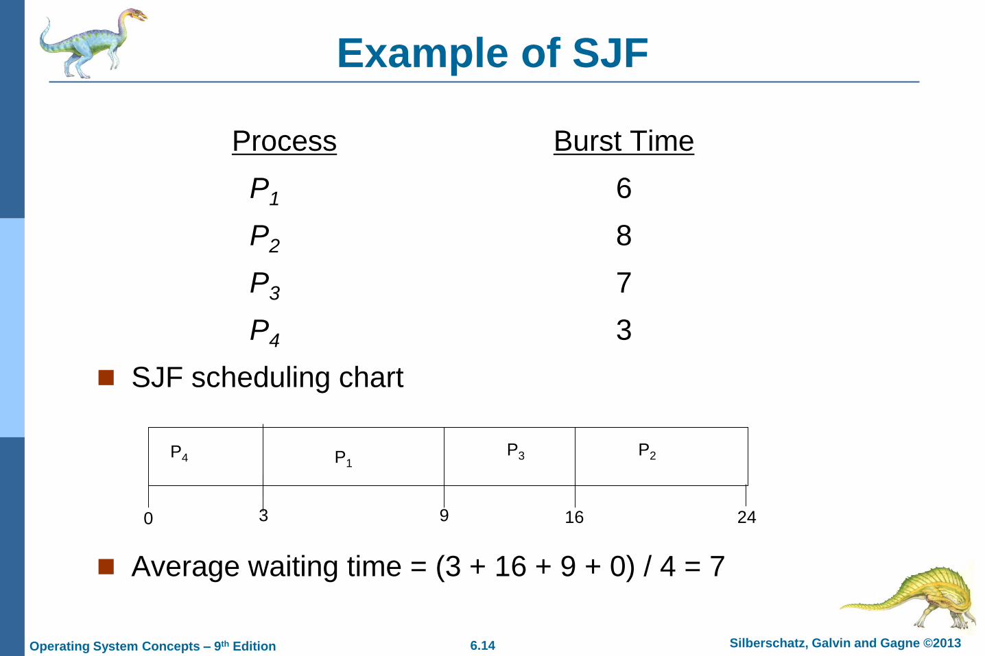
Example of SJF
ProcessArrival Time Burst Time
P1 0.0 6
P2 2.0 8
P3 4.0 7
P4 5.0 3
SJF scheduling chart
Average waiting time = (3 + 16 + 9 + 0) / 4 = 7
P4P3P1
3 160 9
P2
24
6.15 Silberschatz, Galvin and Gagne © 2013Operating System Concepts – 9th Edition
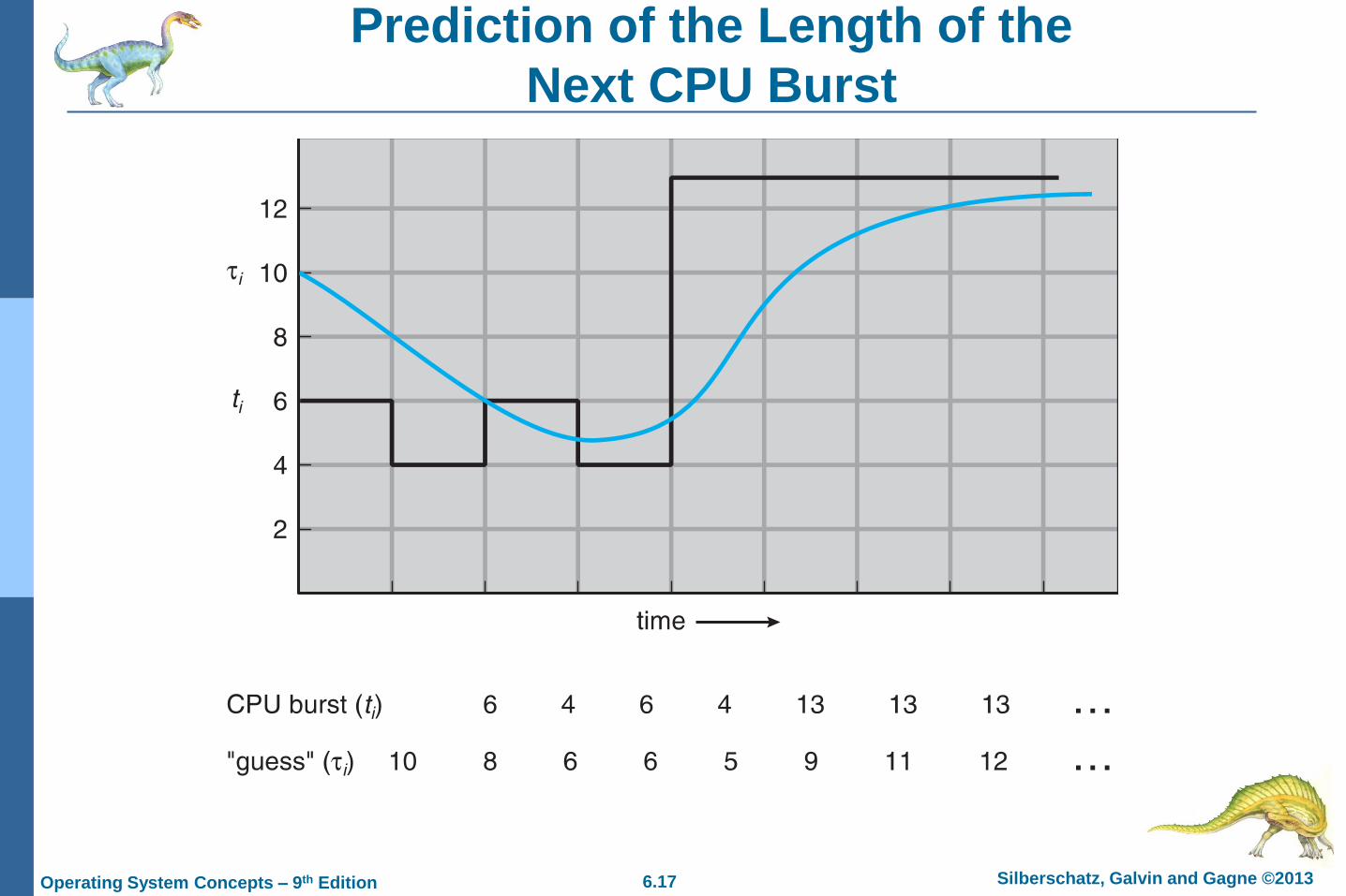
Determining Length of Next CPU Burst
Can only estimate the length – should be similar to the
previous one
Then pick process with shortest predicted next CPU
burst
Can be done by using the length of previous CPU bursts,
using exponential averaging
Commonly, α set to ½
Preemptive version called shortest-remaining-time-first
:Define 4.
10 , 3.
burst CPU next the for value predicted 2.
burst CPU of length actual 1.
1n
thn nt
.1 1 nnn
t
6.16 Silberschatz, Galvin and Gagne © 2013Operating System Concepts – 9th Edition
2014/10/28 stopped here.
6.17 Silberschatz, Galvin and Gagne © 2013Operating System Concepts – 9th Edition
Prediction of the Length of the
Next CPU Burst
6.18 Silberschatz, Galvin and Gagne © 2013Operating System Concepts – 9th Edition
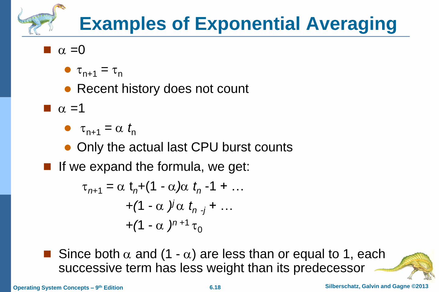
Examples of Exponential Averaging
=0
n+1 = n
Recent history does not count
=1
n+1 = tn
Only the actual last CPU burst counts
If we expand the formula, we get:
n+1 = tn+(1 - ) tn -1 + …
+(1 - )j tn -j + …
+(1 - )n +1 0
Since both and (1 - ) are less than or equal to 1, each successive term has less weight than its predecessor
6.19 Silberschatz, Galvin and Gagne © 2013Operating System Concepts – 9th Edition
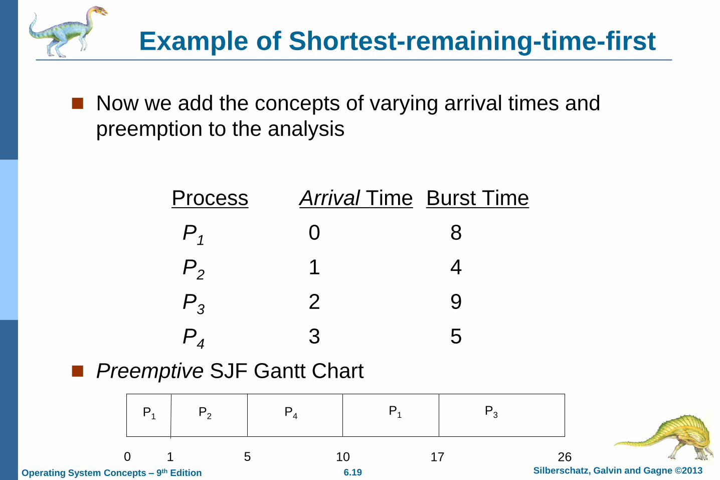
Example of Shortest-remaining-time-first
Now we add the concepts of varying arrival times and
preemption to the analysis
ProcessAarri Arrival TimeTBurst Time
P1 0 8
P2 1 4
P3 2 9
P4 3 5
Preemptive SJF Gantt Chart
P1P1P2
1 170 10
P3
265
P4
6.20 Silberschatz, Galvin and Gagne © 2013Operating System Concepts – 9th Edition
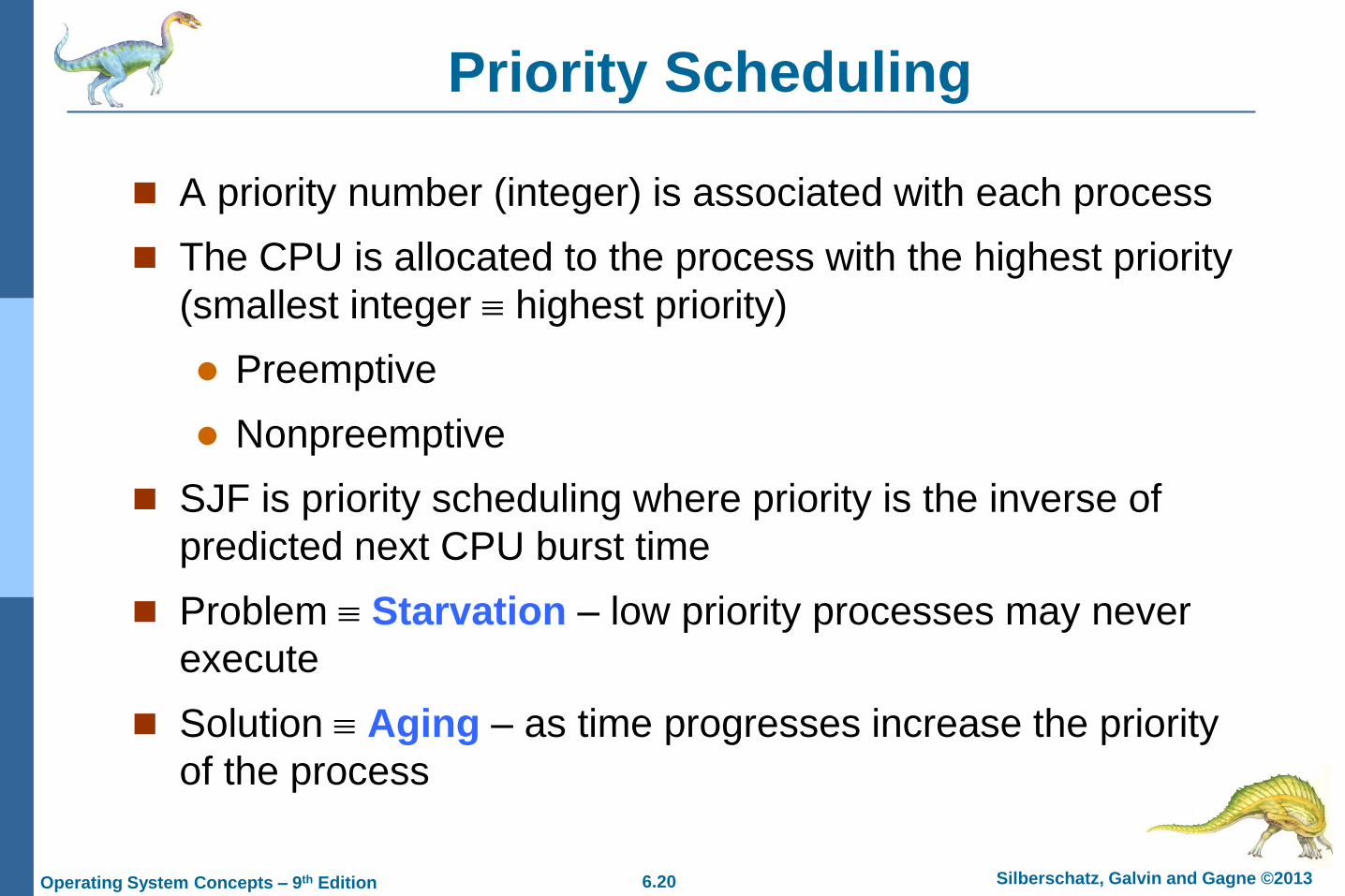
Priority Scheduling
A priority number (integer) is associated with each process
The CPU is allocated to the process with the highest priority
(smallest integer highest priority)
Preemptive
Nonpreemptive
SJF is priority scheduling where priority is the inverse of
predicted next CPU burst time
Problem Starvation – low priority processes may never
execute
Solution Aging – as time progresses increase the priority
of the process
6.21 Silberschatz, Galvin and Gagne © 2013Operating System Concepts – 9th Edition
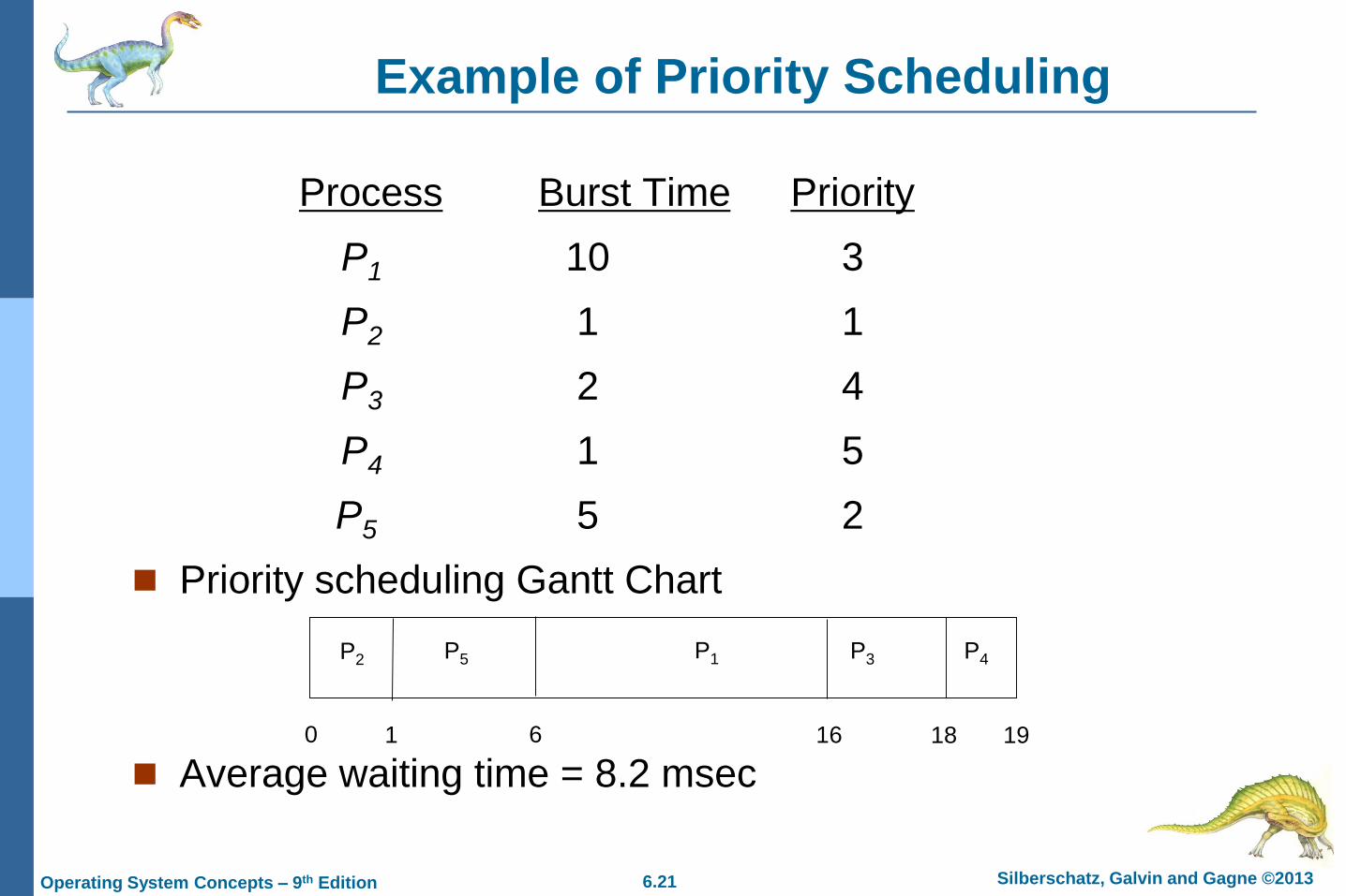
Example of Priority Scheduling
ProcessAarri Burst TimeT Priority
P1 10 3
P2 1 1
P3 2 4
P4 1 5
P5 5 2
Priority scheduling Gantt Chart
Average waiting time = 8.2 msec
P2 P3P5
1 180 16
P4
196
P1
6.22 Silberschatz, Galvin and Gagne © 2013Operating System Concepts – 9th Edition
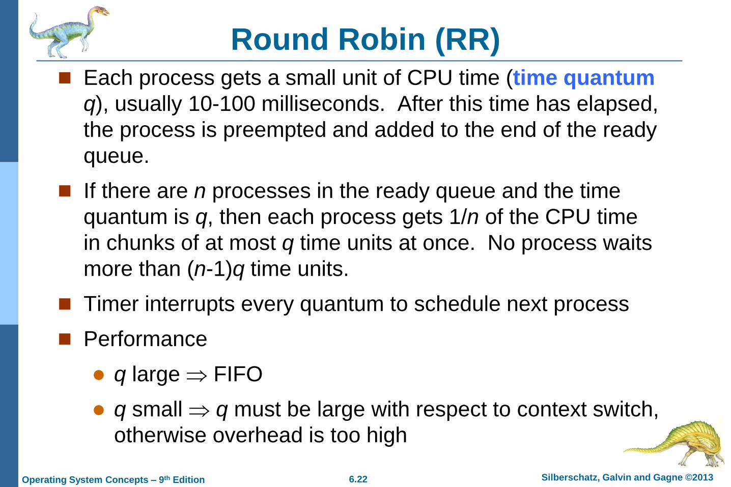
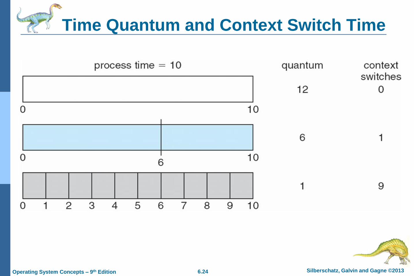
Round Robin (RR) Each process gets a small unit of CPU time (time quantum
q), usually 10-100 milliseconds. After this time has elapsed,
the process is preempted and added to the end of the ready
queue.
If there are n processes in the ready queue and the time
quantum is q, then each process gets 1/n of the CPU time
in chunks of at most q time units at once. No process waits
more than (n-1)q time units.
Timer interrupts every quantum to schedule next process
Performance
q large FIFO
q small q must be large with respect to context switch,
otherwise overhead is too high
6.23 Silberschatz, Galvin and Gagne © 2013Operating System Concepts – 9th Edition
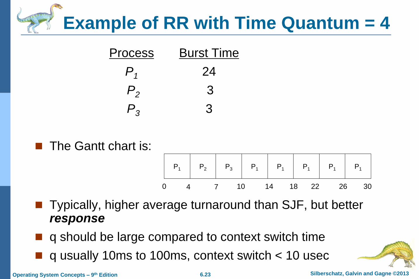
Example of RR with Time Quantum = 4
Process Burst Time
P1 24
P2 3
P3 3
The Gantt chart is:
Typically, higher average turnaround than SJF, but better response
q should be large compared to context switch time
q usually 10ms to 100ms, context switch < 10 usec
P1 P2 P3 P1 P1 P1 P1 P1
0 4 7 10 14 18 22 26 30
6.24 Silberschatz, Galvin and Gagne © 2013Operating System Concepts – 9th Edition
Time Quantum and Context Switch Time
6.25 Silberschatz, Galvin and Gagne © 2013Operating System Concepts – 9th Edition
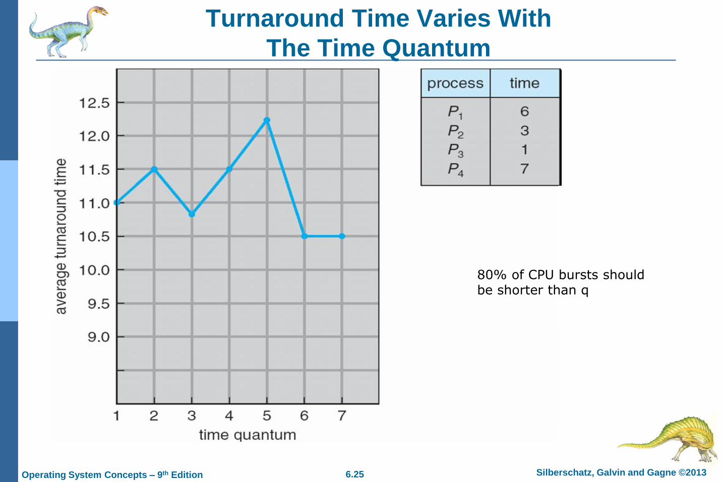
Turnaround Time Varies With
The Time Quantum
80% of CPU bursts should be shorter than q
6.26 Silberschatz, Galvin and Gagne © 2013Operating System Concepts – 9th Edition
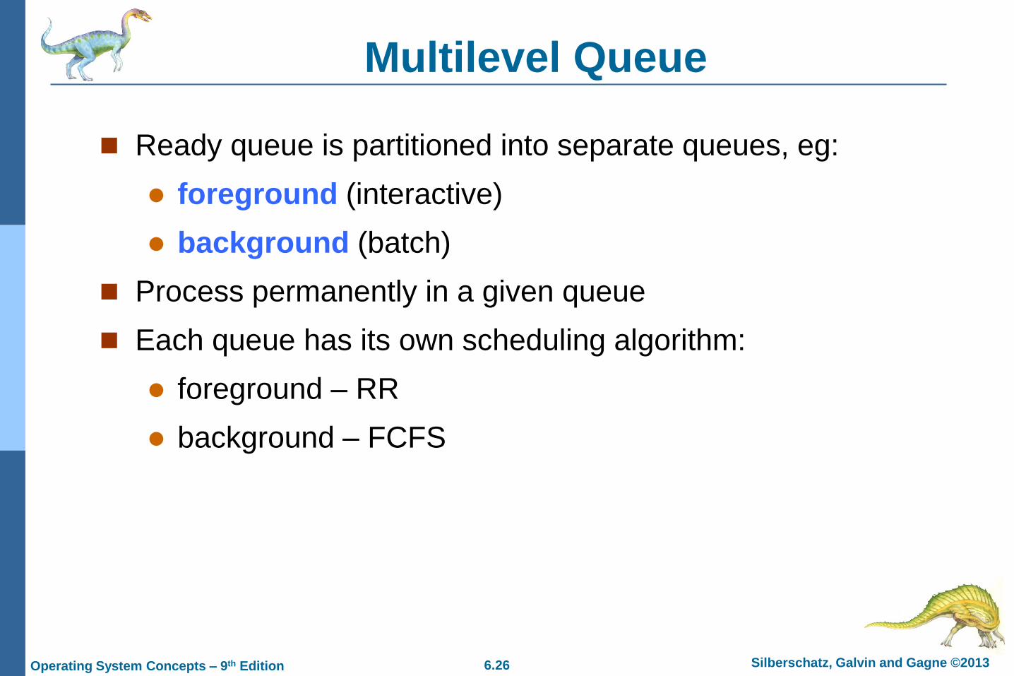
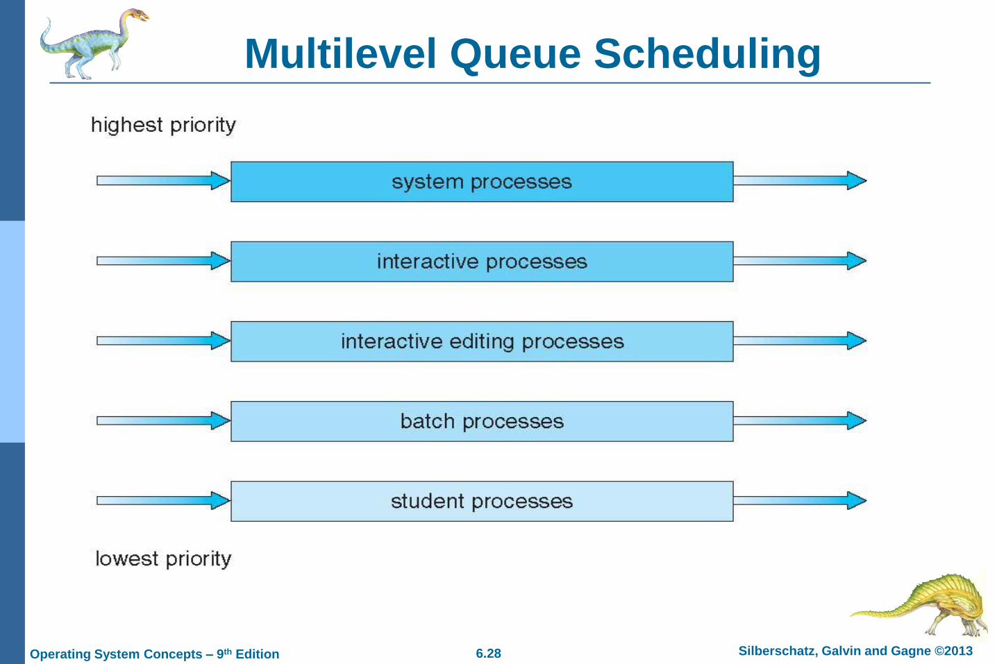
Multilevel Queue
Ready queue is partitioned into separate queues, eg:
foreground (interactive)
background (batch)
Process permanently in a given queue
Each queue has its own scheduling algorithm:
foreground – RR
background – FCFS

6.27 Silberschatz, Galvin and Gagne © 2013Operating System Concepts – 9th Edition
Multilevel Queue
Scheduling must be done between the queues:
Fixed priority scheduling; (i.e., serve all from foreground
then from background). Possibility of starvation.
Time slice – each queue gets a certain amount of CPU
time which it can schedule amongst its processes; i.e.,
80% to foreground in RR
20% to background in FCFS
6.28 Silberschatz, Galvin and Gagne © 2013Operating System Concepts – 9th Edition
Multilevel Queue Scheduling
6.29 Silberschatz, Galvin and Gagne © 2013Operating System Concepts – 9th Edition
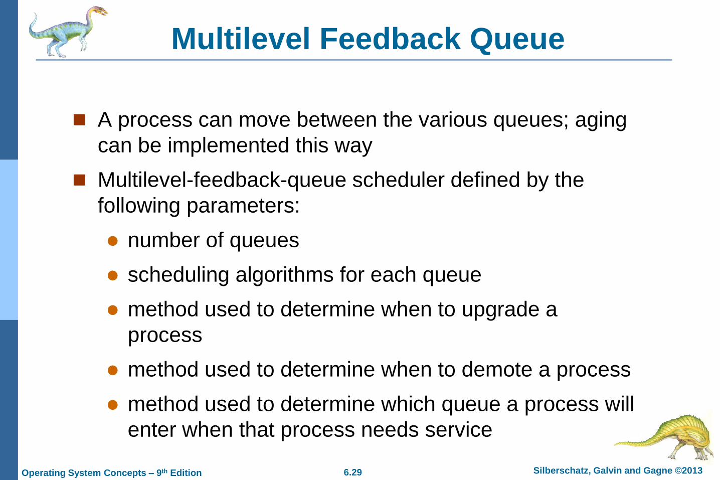
Multilevel Feedback Queue
A process can move between the various queues; aging
can be implemented this way
Multilevel-feedback-queue scheduler defined by the
following parameters:
number of queues
scheduling algorithms for each queue
method used to determine when to upgrade a
process
method used to determine when to demote a process
method used to determine which queue a process will
enter when that process needs service
6.30 Silberschatz, Galvin and Gagne © 2013Operating System Concepts – 9th Edition
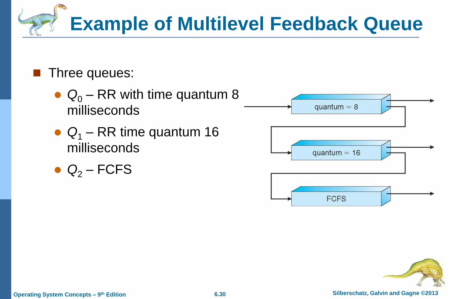
Example of Multilevel Feedback Queue
Three queues:
Q0 – RR with time quantum 8
milliseconds
Q1 – RR time quantum 16
milliseconds
Q2 – FCFS
6.31 Silberschatz, Galvin and Gagne © 2013Operating System Concepts – 9th Edition
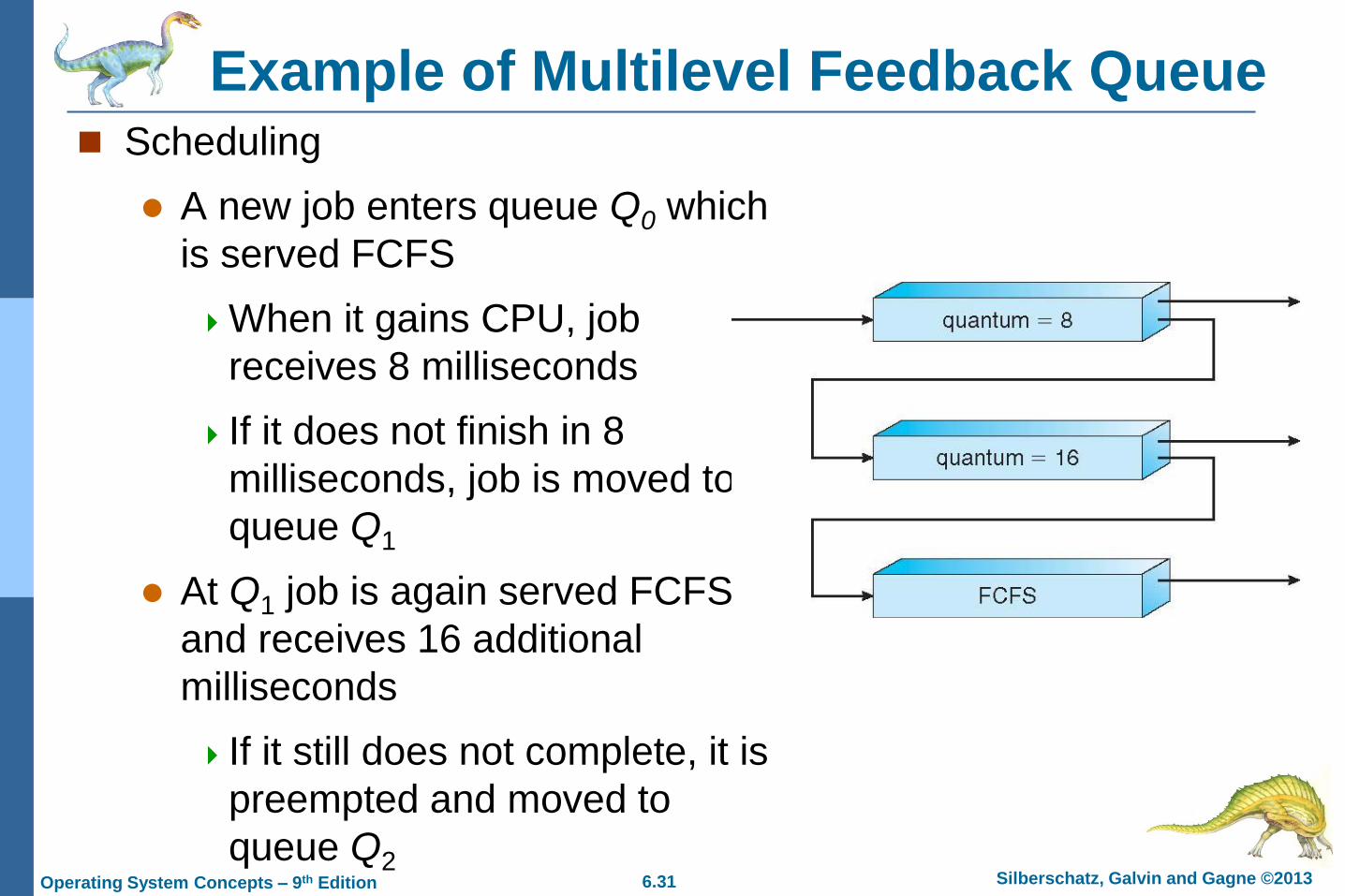
Example of Multilevel Feedback Queue Scheduling
A new job enters queue Q0 which
is served FCFS
When it gains CPU, job
receives 8 milliseconds
If it does not finish in 8
milliseconds, job is moved to
queue Q1
At Q1 job is again served FCFS
and receives 16 additional
milliseconds
If it still does not complete, it is
preempted and moved to
queue Q2
6.32 Silberschatz, Galvin and Gagne © 2013Operating System Concepts – 9th Edition
Thread Scheduling (胡明衛)
Distinction between user-level and kernel-level threads
When threads supported, threads scheduled, not processes
Many-to-one and many-to-many models, thread library
schedules user-level threads to run on LWP
Known as process-contention scope (PCS) since
scheduling competition is within the process
Typically done via priority set by programmer
Kernel thread scheduled onto available CPU is system-
contention scope (SCS) – competition among all threads
in system
6.33 Silberschatz, Galvin and Gagne © 2013Operating System Concepts – 9th Edition
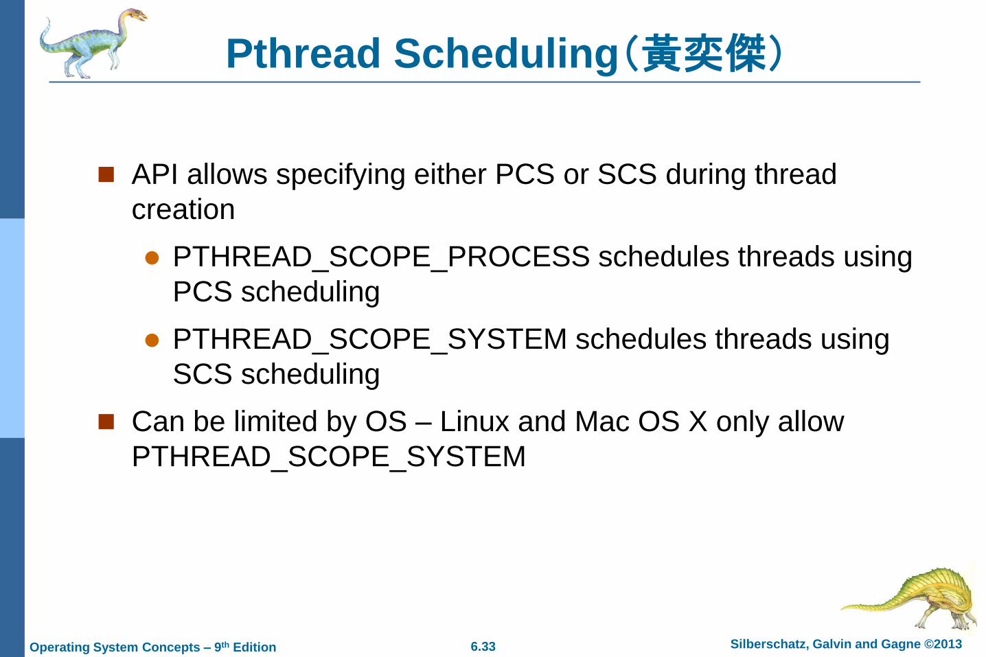
Pthread Scheduling(黃奕傑)
API allows specifying either PCS or SCS during thread
creation
PTHREAD_SCOPE_PROCESS schedules threads using
PCS scheduling
PTHREAD_SCOPE_SYSTEM schedules threads using
SCS scheduling
Can be limited by OS – Linux and Mac OS X only allow
PTHREAD_SCOPE_SYSTEM
6.34 Silberschatz, Galvin and Gagne © 2013Operating System Concepts – 9th Edition
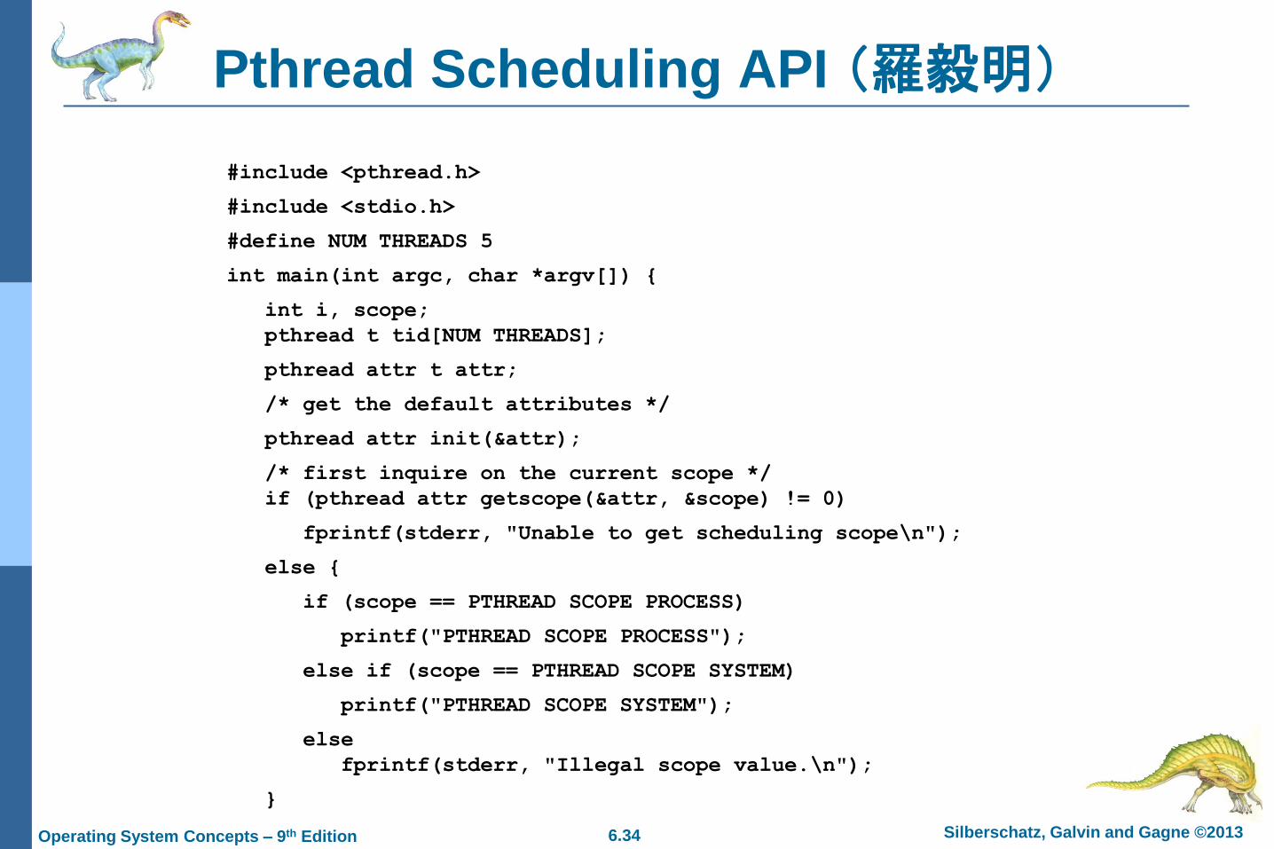
Pthread Scheduling API (羅毅明)
#include <pthread.h>
#include <stdio.h>
#define NUM THREADS 5
int main(int argc, char *argv[]) {
int i, scope;
pthread t tid[NUM THREADS];
pthread attr t attr;
/* get the default attributes */
pthread attr init(&attr);
/* first inquire on the current scope */
if (pthread attr getscope(&attr, &scope) != 0)
fprintf(stderr, "Unable to get scheduling scope\n");
else {
if (scope == PTHREAD SCOPE PROCESS)
printf("PTHREAD SCOPE PROCESS");
else if (scope == PTHREAD SCOPE SYSTEM)
printf("PTHREAD SCOPE SYSTEM");
else
fprintf(stderr, "Illegal scope value.\n");
}
6.35 Silberschatz, Galvin and Gagne © 2013Operating System Concepts – 9th Edition
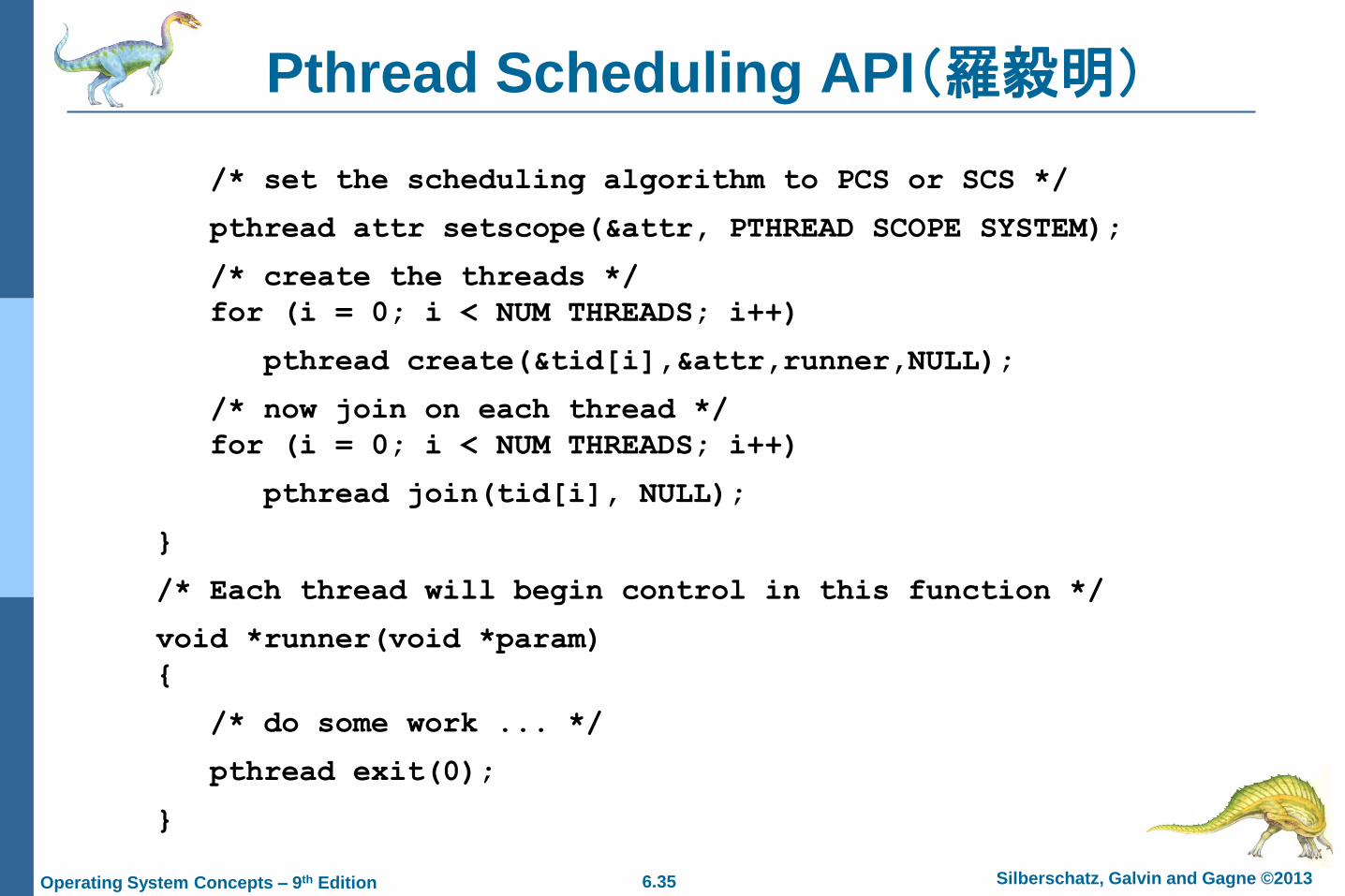
Pthread Scheduling API(羅毅明)
/* set the scheduling algorithm to PCS or SCS */
pthread attr setscope(&attr, PTHREAD SCOPE SYSTEM);
/* create the threads */
for (i = 0; i < NUM THREADS; i++)
pthread create(&tid[i],&attr,runner,NULL);
/* now join on each thread */
for (i = 0; i < NUM THREADS; i++)
pthread join(tid[i], NULL);
}
/* Each thread will begin control in this function */
void *runner(void *param)
{
/* do some work ... */
pthread exit(0);
}
6.36 Silberschatz, Galvin and Gagne © 2013Operating System Concepts – 9th Edition
Multiple-Processor Scheduling
CPU scheduling more complex when multiple CPUs are
available
Homogeneous processors within a multiprocessor
Asymmetric multiprocessing – only one processor accesses
the system data structures, alleviating the need for data
sharing
Symmetric multiprocessing (SMP) – each processor is self-
scheduling, all processes in common ready queue, or each has
its own private queue of ready processes
Currently, most common
6.37 Silberschatz, Galvin and Gagne © 2013Operating System Concepts – 9th Edition
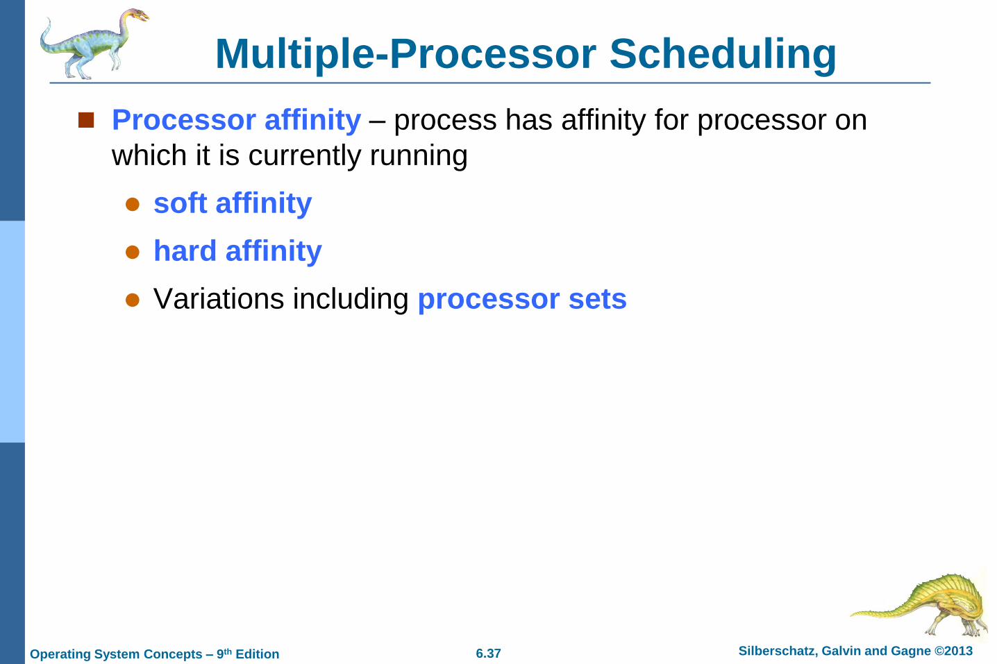
Multiple-Processor Scheduling
Processor affinity – process has affinity for processor on
which it is currently running
soft affinity
hard affinity
Variations including processor sets
6.38 Silberschatz, Galvin and Gagne © 2013Operating System Concepts – 9th Edition
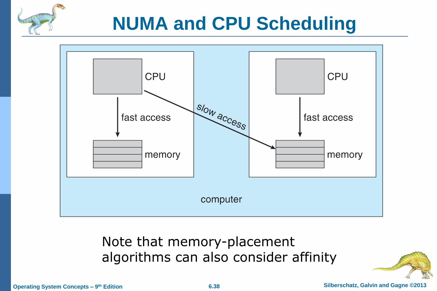
NUMA and CPU Scheduling
Note that memory-placement algorithms can also consider affinity
6.39 Silberschatz, Galvin and Gagne © 2013Operating System Concepts – 9th Edition
Multiple-Processor Scheduling – Load Balancing
If SMP, need to keep all CPUs loaded for efficiency
Load balancing attempts to keep workload evenly distributed
Push migration – periodic task checks load on each processor, and if found pushes task from
overloaded CPU to other CPUs
Pull migration – idle processors pulls waiting task from busy processor
6.40 Silberschatz, Galvin and Gagne © 2013Operating System Concepts – 9th Edition
5.08
6.41 Silberschatz, Galvin and Gagne © 2013Operating System Concepts – 9th Edition
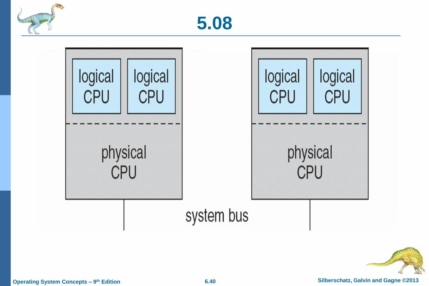
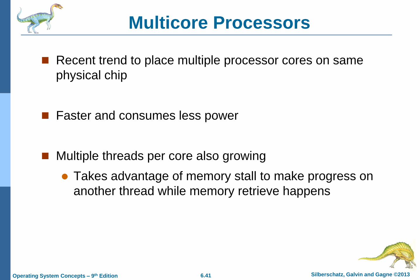
Multicore Processors
Recent trend to place multiple processor cores on same
physical chip
Faster and consumes less power
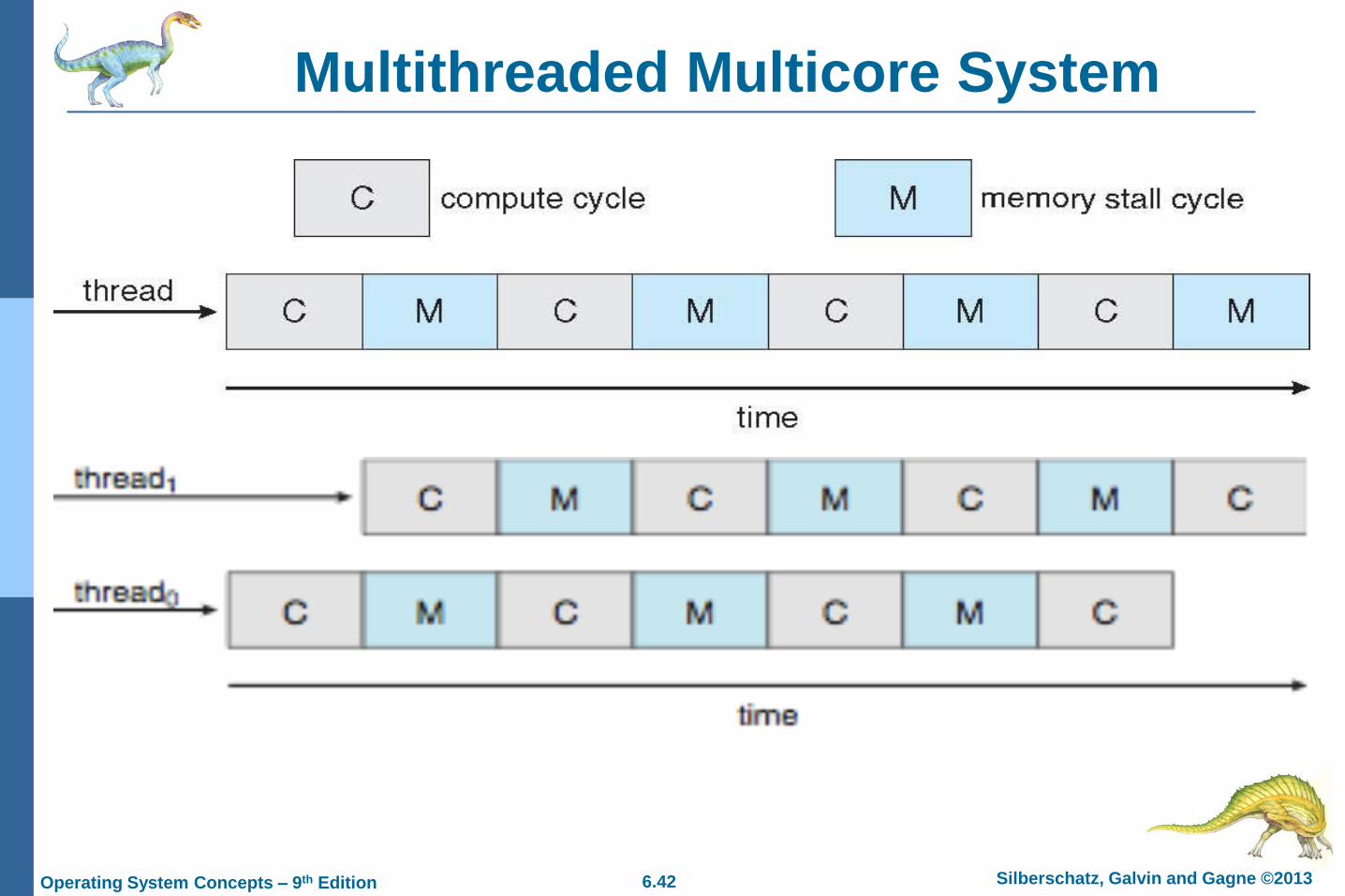
Multiple threads per core also growing
Takes advantage of memory stall to make progress on
another thread while memory retrieve happens
6.42 Silberschatz, Galvin and Gagne © 2013Operating System Concepts – 9th Edition
Multithreaded Multicore System
6.43 Silberschatz, Galvin and Gagne © 2013Operating System Concepts – 9th Edition
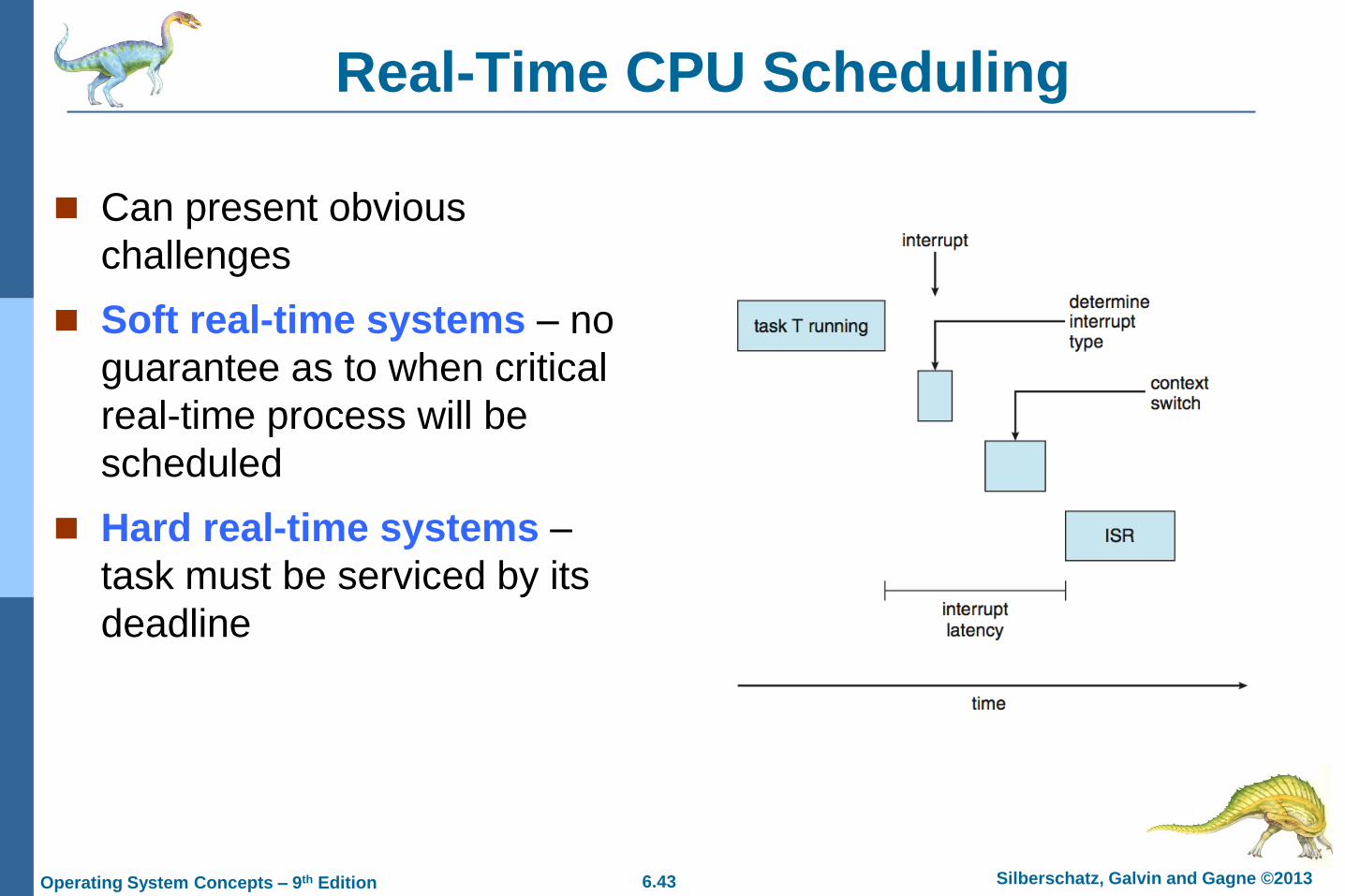
Real-Time CPU Scheduling
Can present obvious
challenges
Soft real-time systems – no
guarantee as to when critical
real-time process will be
scheduled
Hard real-time systems –
task must be serviced by its
deadline
6.44 Silberschatz, Galvin and Gagne © 2013Operating System Concepts – 9th Edition
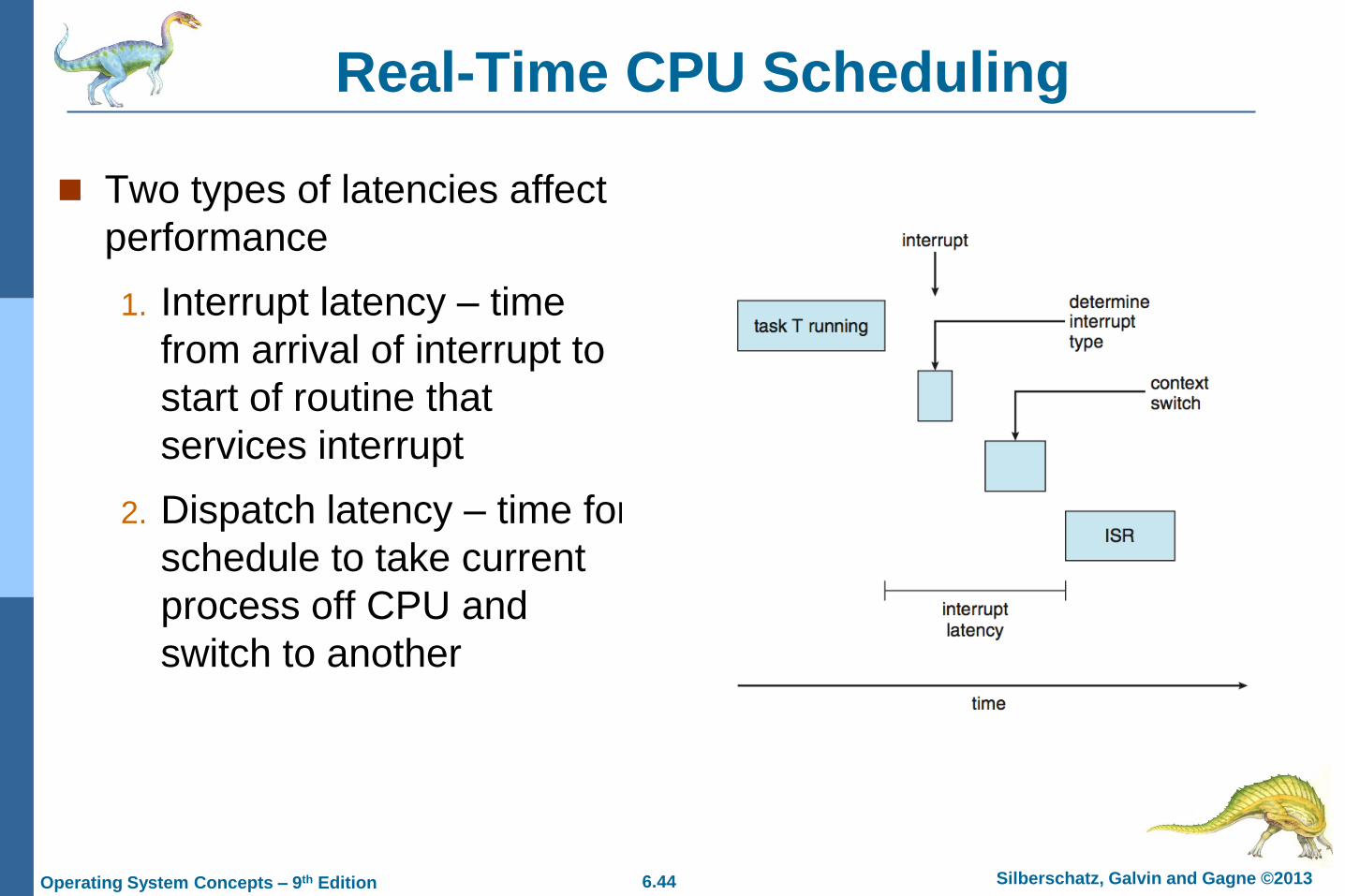
Real-Time CPU Scheduling
Two types of latencies affect
performance
1. Interrupt latency – time
from arrival of interrupt to
start of routine that
services interrupt
2. Dispatch latency – time for
schedule to take current
process off CPU and
switch to another

6.45 Silberschatz, Galvin and Gagne © 2013Operating System Concepts – 9th Edition
Real-Time CPU Scheduling (Cont.)
Conflict phase of
dispatch latency:
1. Preemption of any
process running in
kernel mode
2. Release by low-
priority process of
resources needed
by high-priority
processes
6.46 Silberschatz, Galvin and Gagne © 2013Operating System Concepts – 9th Edition
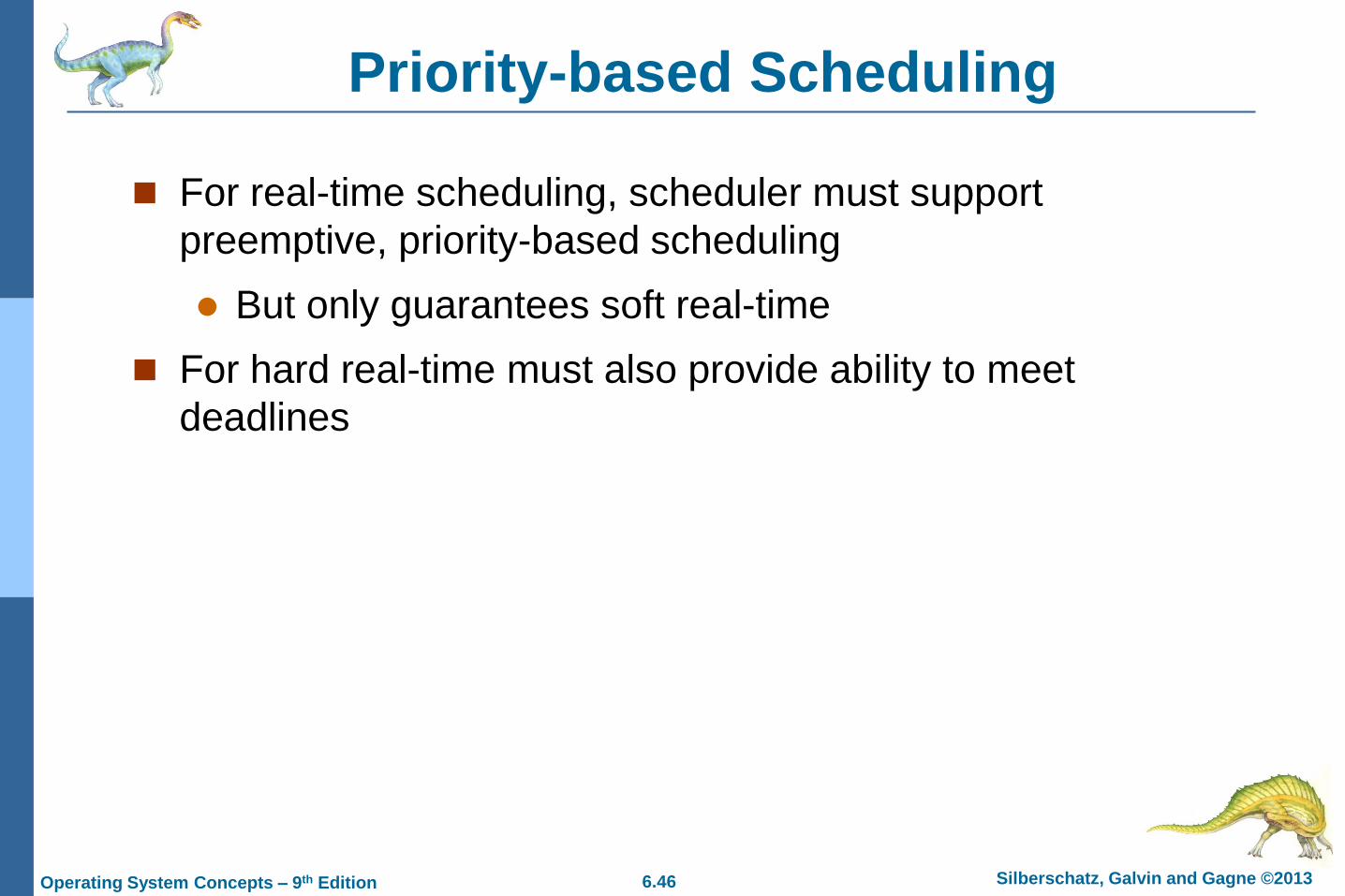
Priority-based Scheduling
For real-time scheduling, scheduler must support
preemptive, priority-based scheduling
But only guarantees soft real-time
For hard real-time must also provide ability to meet
deadlines
6.47 Silberschatz, Galvin and Gagne © 2013Operating System Concepts – 9th Edition
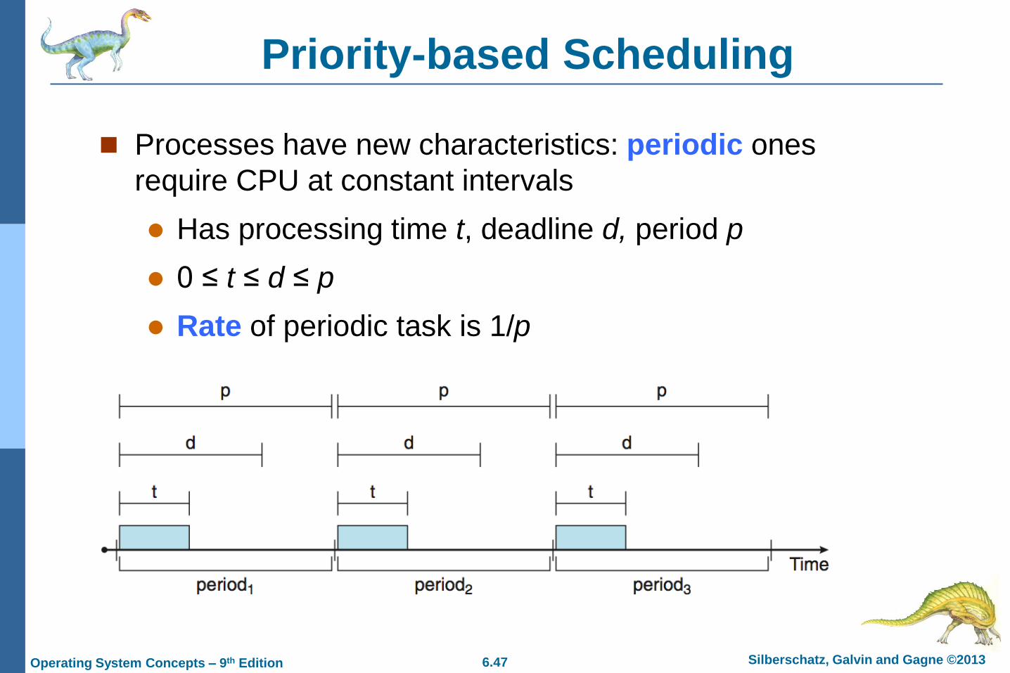
Priority-based Scheduling
Processes have new characteristics: periodic ones
require CPU at constant intervals
Has processing time t, deadline d, period p
0 ≤ t ≤ d ≤ p
Rate of periodic task is 1/p
6.48 Silberschatz, Galvin and Gagne © 2013Operating System Concepts – 9th Edition
Virtualization and Scheduling
Virtualization software schedules multiple guests onto CPU(s)
Each guest doing its own scheduling
Not knowing it doesn’t own the CPUs
Can result in poor response time
Can effect time-of-day clocks in guests
Can undo good scheduling algorithm efforts of guests
6.49 Silberschatz, Galvin and Gagne © 2013Operating System Concepts – 9th Edition
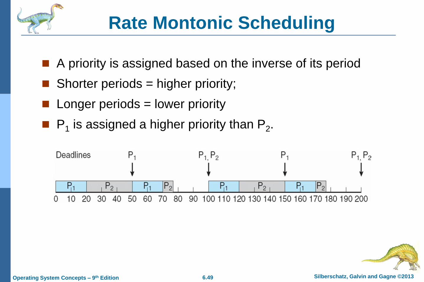
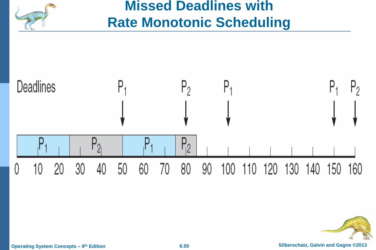
Rate Montonic Scheduling
A priority is assigned based on the inverse of its period
Shorter periods = higher priority;
Longer periods = lower priority
P1 is assigned a higher priority than P2.
6.50 Silberschatz, Galvin and Gagne © 2013Operating System Concepts – 9th Edition
Missed Deadlines with
Rate Monotonic Scheduling

6.51 Silberschatz, Galvin and Gagne © 2013Operating System Concepts – 9th Edition
Earliest Deadline First Scheduling (EDF)
Priorities are assigned according to deadlines:
the earlier the deadline, the higher the priority;
the later the deadline, the lower the priority
6.52 Silberschatz, Galvin and Gagne © 2013Operating System Concepts – 9th Edition
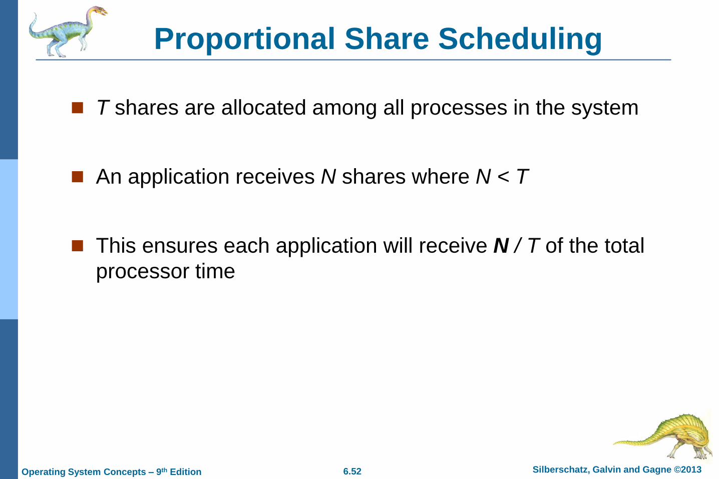
Proportional Share Scheduling
T shares are allocated among all processes in the system
An application receives N shares where N < T
This ensures each application will receive N / T of the total
processor time
6.53 Silberschatz, Galvin and Gagne © 2013Operating System Concepts – 9th Edition
POSIX Real-Time Scheduling
The POSIX.1b standard
API provides functions for managing real-time threads
Defines two scheduling classes for real-time threads:
1. SCHED_FIFO - threads are scheduled using a FCFS
strategy with a FIFO queue. There is no time-slicing for
threads of equal priority
2. SCHED_RR - similar to SCHED_FIFO except time-slicing
occurs for threads of equal priority
6.54 Silberschatz, Galvin and Gagne © 2013Operating System Concepts – 9th Edition
POSIX Real-Time Scheduling
Defines two functions for getting and setting scheduling
policy:
1.pthread attr getsched policy(pthread attr t
*attr, int *policy)
2.pthread attr setsched policy(pthread attr t
*attr, int policy)
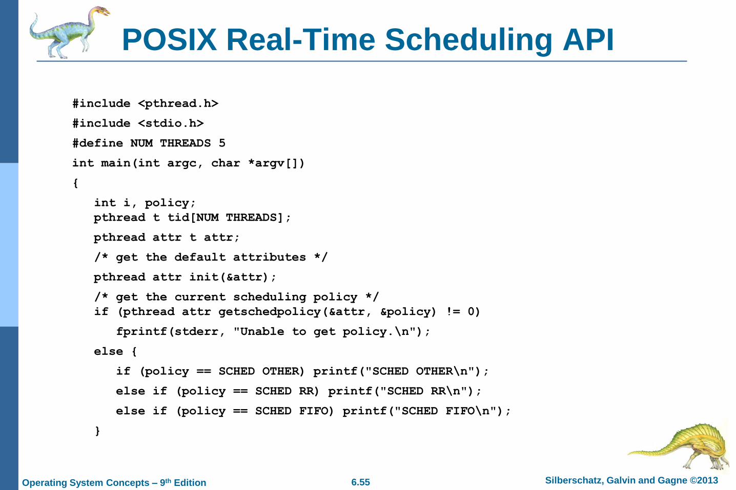
6.55 Silberschatz, Galvin and Gagne © 2013Operating System Concepts – 9th Edition
POSIX Real-Time Scheduling API
#include <pthread.h>
#include <stdio.h>
#define NUM THREADS 5
int main(int argc, char *argv[])
{
int i, policy;
pthread t tid[NUM THREADS];
pthread attr t attr;
/* get the default attributes */
pthread attr init(&attr);
/* get the current scheduling policy */
if (pthread attr getschedpolicy(&attr, &policy) != 0)
fprintf(stderr, "Unable to get policy.\n");
else {
if (policy == SCHED OTHER) printf("SCHED OTHER\n");
else if (policy == SCHED RR) printf("SCHED RR\n");
else if (policy == SCHED FIFO) printf("SCHED FIFO\n");
}
6.56 Silberschatz, Galvin and Gagne © 2013Operating System Concepts – 9th Edition
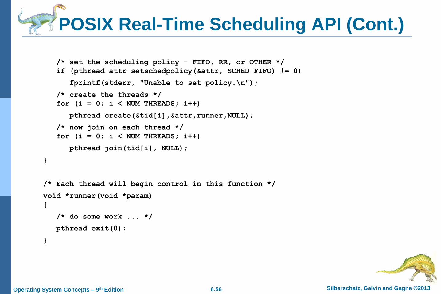
POSIX Real-Time Scheduling API (Cont.)
/* set the scheduling policy - FIFO, RR, or OTHER */
if (pthread attr setschedpolicy(&attr, SCHED FIFO) != 0)
fprintf(stderr, "Unable to set policy.\n");
/* create the threads */
for (i = 0; i < NUM THREADS; i++)
pthread create(&tid[i],&attr,runner,NULL);
/* now join on each thread */
for (i = 0; i < NUM THREADS; i++)
pthread join(tid[i], NULL);
}
/* Each thread will begin control in this function */
void *runner(void *param)
{
/* do some work ... */
pthread exit(0);
}
6.57 Silberschatz, Galvin and Gagne © 2013Operating System Concepts – 9th Edition
Operating System Examples
Linux scheduling
Windows scheduling
Solaris scheduling
6.58 Silberschatz, Galvin and Gagne © 2013Operating System Concepts – 9th Edition
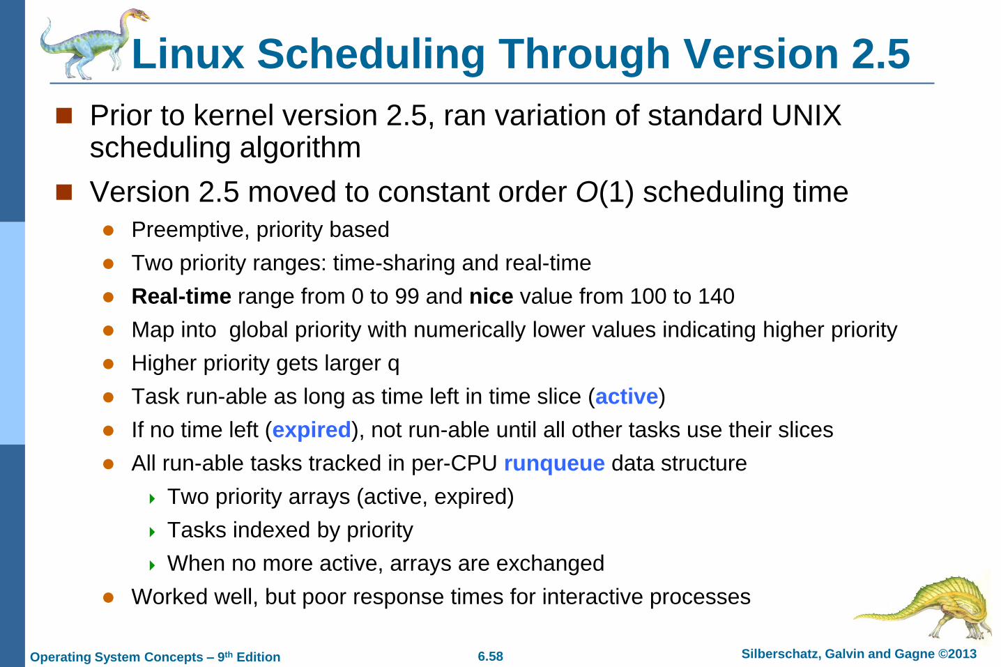
Linux Scheduling Through Version 2.5
Prior to kernel version 2.5, ran variation of standard UNIX scheduling algorithm
Version 2.5 moved to constant order O(1) scheduling time
Preemptive, priority based
Two priority ranges: time-sharing and real-time
Real-time range from 0 to 99 and nice value from 100 to 140
Map into global priority with numerically lower values indicating higher priority
Higher priority gets larger q
Task run-able as long as time left in time slice (active)
If no time left (expired), not run-able until all other tasks use their slices
All run-able tasks tracked in per-CPU runqueue data structure
Two priority arrays (active, expired)
Tasks indexed by priority
When no more active, arrays are exchanged
Worked well, but poor response times for interactive processes
6.59 Silberschatz, Galvin and Gagne © 2013Operating System Concepts – 9th Edition
Linux Scheduling in Version 2.6.23 +
Completely Fair Scheduler (CFS)
Scheduling classes
Each has specific priority
Scheduler picks highest priority task in highest scheduling class
Rather than quantum based on fixed time allotments, based on proportion of CPU time
2 scheduling classes included, others can be added
1. default
2. real-time
6.60 Silberschatz, Galvin and Gagne © 2013Operating System Concepts – 9th Edition
Linux Scheduling in Version 2.6.23 + Quantum calculated based on nice value from -20 to
+19
Lower value is higher priority
Calculates target latency – interval of time during which task should run at least once
Target latency can increase if say number of active tasks increases
CFS scheduler maintains per task virtual run time in variable vruntime
Associated with decay factor based on priority of task – lower priority is higher decay rate
Normal default priority yields virtual run time = actual run time
To decide next task to run, scheduler picks task with lowest virtual run time
6.61 Silberschatz, Galvin and Gagne © 2013Operating System Concepts – 9th Edition
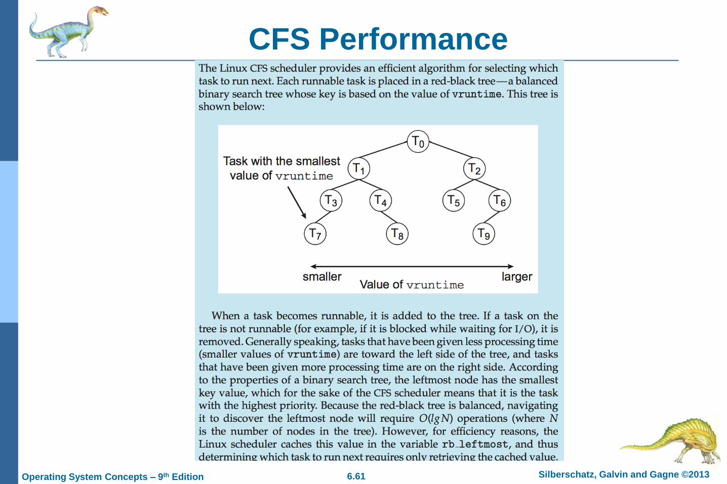
CFS Performance

6.62 Silberschatz, Galvin and Gagne © 2013Operating System Concepts – 9th Edition
Linux Scheduling (Cont.)
Real-time scheduling according to POSIX.1b
Real-time tasks have static priorities
Real-time plus normal map into global priority scheme
Nice value of -20 maps to global priority 100
Nice value of +19 maps to priority 139
6.63 Silberschatz, Galvin and Gagne © 2013Operating System Concepts – 9th Edition
Windows Scheduling Windows uses priority-based preemptive scheduling
Highest-priority thread runs next
Dispatcher is scheduler
Thread runs until (1) blocks, (2) uses time slice, (3) preempted
by higher-priority thread
Real-time threads can preempt non-real-time
32-level priority scheme
Variable class is 1-15, real-time class is 16-31
Priority 0 is memory-management thread
Queue for each priority
If no run-able thread, runs idle thread
6.64 Silberschatz, Galvin and Gagne © 2013Operating System Concepts – 9th Edition
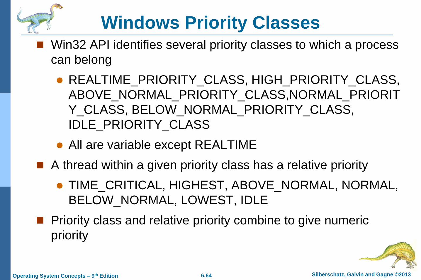
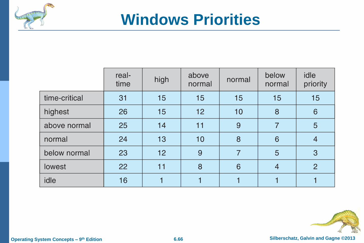
Windows Priority Classes Win32 API identifies several priority classes to which a process
can belong
REALTIME_PRIORITY_CLASS, HIGH_PRIORITY_CLASS,
ABOVE_NORMAL_PRIORITY_CLASS,NORMAL_PRIORIT
Y_CLASS, BELOW_NORMAL_PRIORITY_CLASS,
IDLE_PRIORITY_CLASS
All are variable except REALTIME
A thread within a given priority class has a relative priority
TIME_CRITICAL, HIGHEST, ABOVE_NORMAL, NORMAL,
BELOW_NORMAL, LOWEST, IDLE
Priority class and relative priority combine to give numeric
priority
6.65 Silberschatz, Galvin and Gagne © 2013Operating System Concepts – 9th Edition
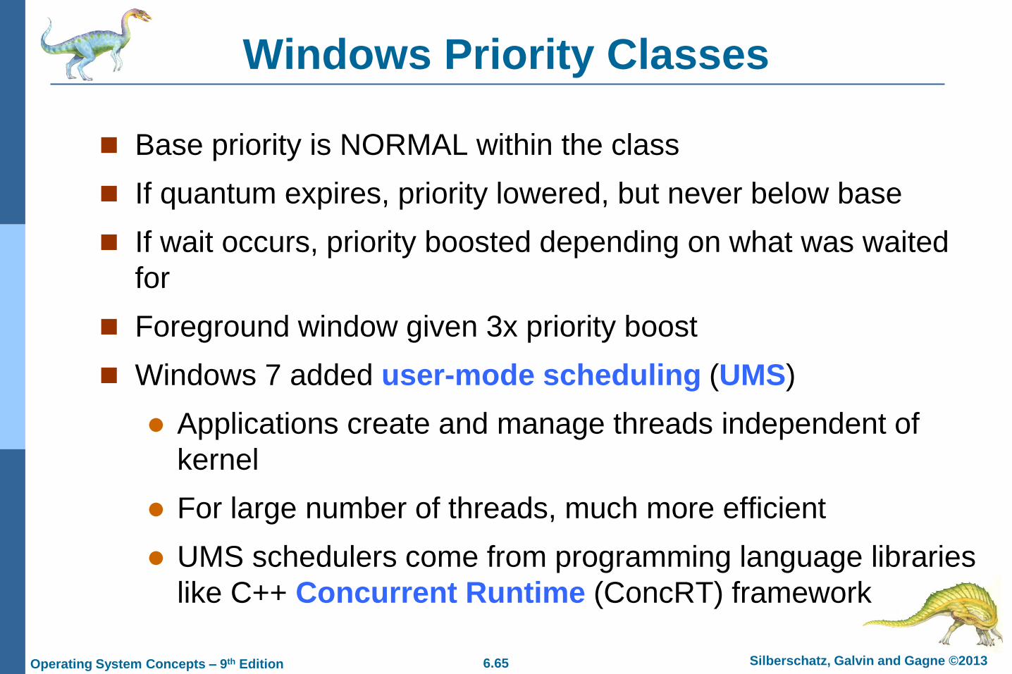
Windows Priority Classes
Base priority is NORMAL within the class
If quantum expires, priority lowered, but never below base
If wait occurs, priority boosted depending on what was waited
for
Foreground window given 3x priority boost
Windows 7 added user-mode scheduling (UMS)
Applications create and manage threads independent of
kernel
For large number of threads, much more efficient
UMS schedulers come from programming language libraries
like C++ Concurrent Runtime (ConcRT) framework
6.66 Silberschatz, Galvin and Gagne © 2013Operating System Concepts – 9th Edition
Windows Priorities
6.67 Silberschatz, Galvin and Gagne © 2013Operating System Concepts – 9th Edition
Solaris Priority-based scheduling
Six classes available
Time sharing (default) (TS)
Interactive (IA)
Real time (RT)
System (SYS)
Fair Share (FSS)
Fixed priority (FP)
Given thread can be in one class at a time
Each class has its own scheduling algorithm
Time sharing is multi-level feedback queue
Loadable table configurable by sysadmin
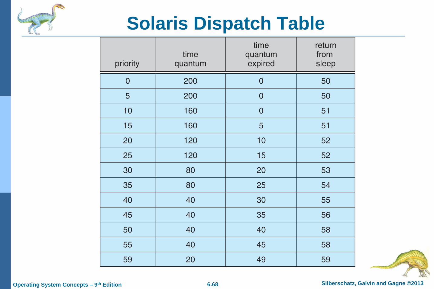
6.68 Silberschatz, Galvin and Gagne © 2013Operating System Concepts – 9th Edition
Solaris Dispatch Table
6.69 Silberschatz, Galvin and Gagne © 2013Operating System Concepts – 9th Edition
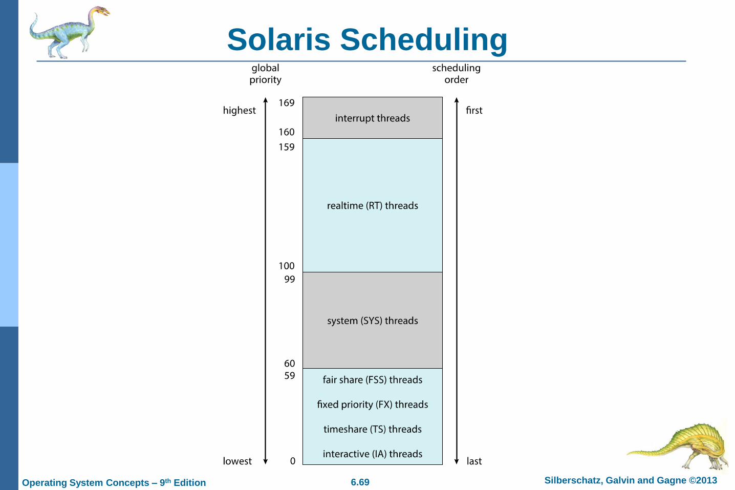
Solaris Scheduling
6.70 Silberschatz, Galvin and Gagne © 2013Operating System Concepts – 9th Edition
Solaris Scheduling (Cont.)
Scheduler converts class-specific priorities into a per-thread
global priority
Thread with highest priority runs next
Runs until (1) blocks, (2) uses time slice, (3) preempted by
higher-priority thread
Multiple threads at same priority selected via RR
6.71 Silberschatz, Galvin and Gagne © 2013Operating System Concepts – 9th Edition
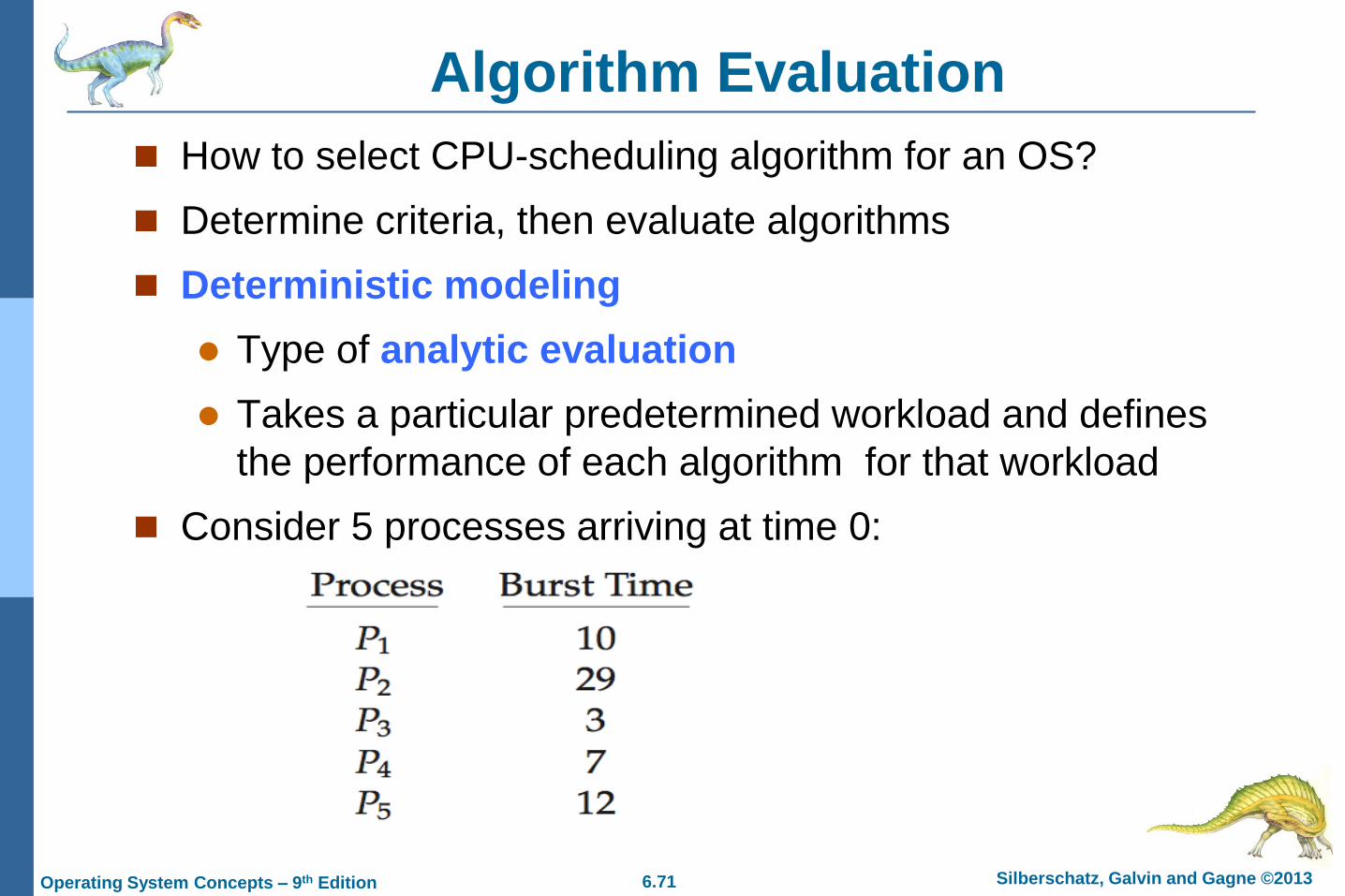
Algorithm Evaluation
How to select CPU-scheduling algorithm for an OS?
Determine criteria, then evaluate algorithms
Deterministic modeling
Type of analytic evaluation
Takes a particular predetermined workload and defines
the performance of each algorithm for that workload
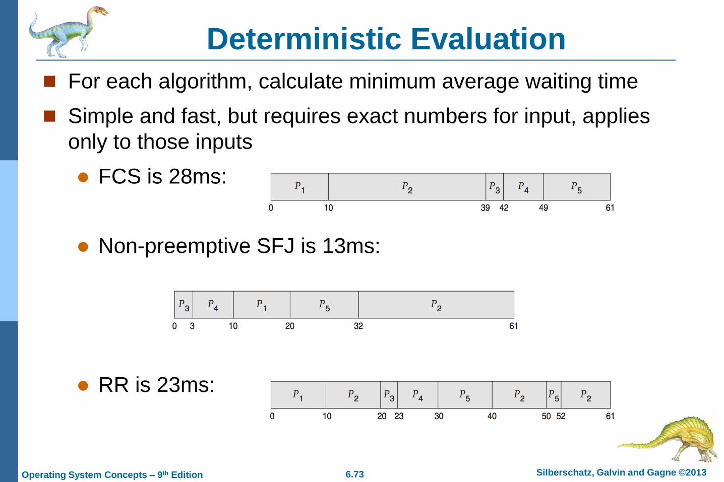
Consider 5 processes arriving at time 0:
6.72 Silberschatz, Galvin and Gagne © 2013Operating System Concepts – 9th Edition
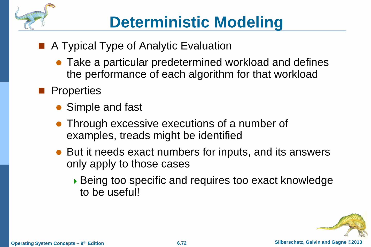
Deterministic Modeling
A Typical Type of Analytic Evaluation
Take a particular predetermined workload and defines the performance of each algorithm for that workload
Properties
Simple and fast
Through excessive executions of a number of examples, treads might be identified
But it needs exact numbers for inputs, and its answers only apply to those cases
Being too specific and requires too exact knowledge to be useful!
6.73 Silberschatz, Galvin and Gagne © 2013Operating System Concepts – 9th Edition
Deterministic Evaluation
For each algorithm, calculate minimum average waiting time
Simple and fast, but requires exact numbers for input, applies
only to those inputs
FCS is 28ms:
Non-preemptive SFJ is 13ms:
RR is 23ms:
6.74 Silberschatz, Galvin and Gagne © 2013Operating System Concepts – 9th Edition
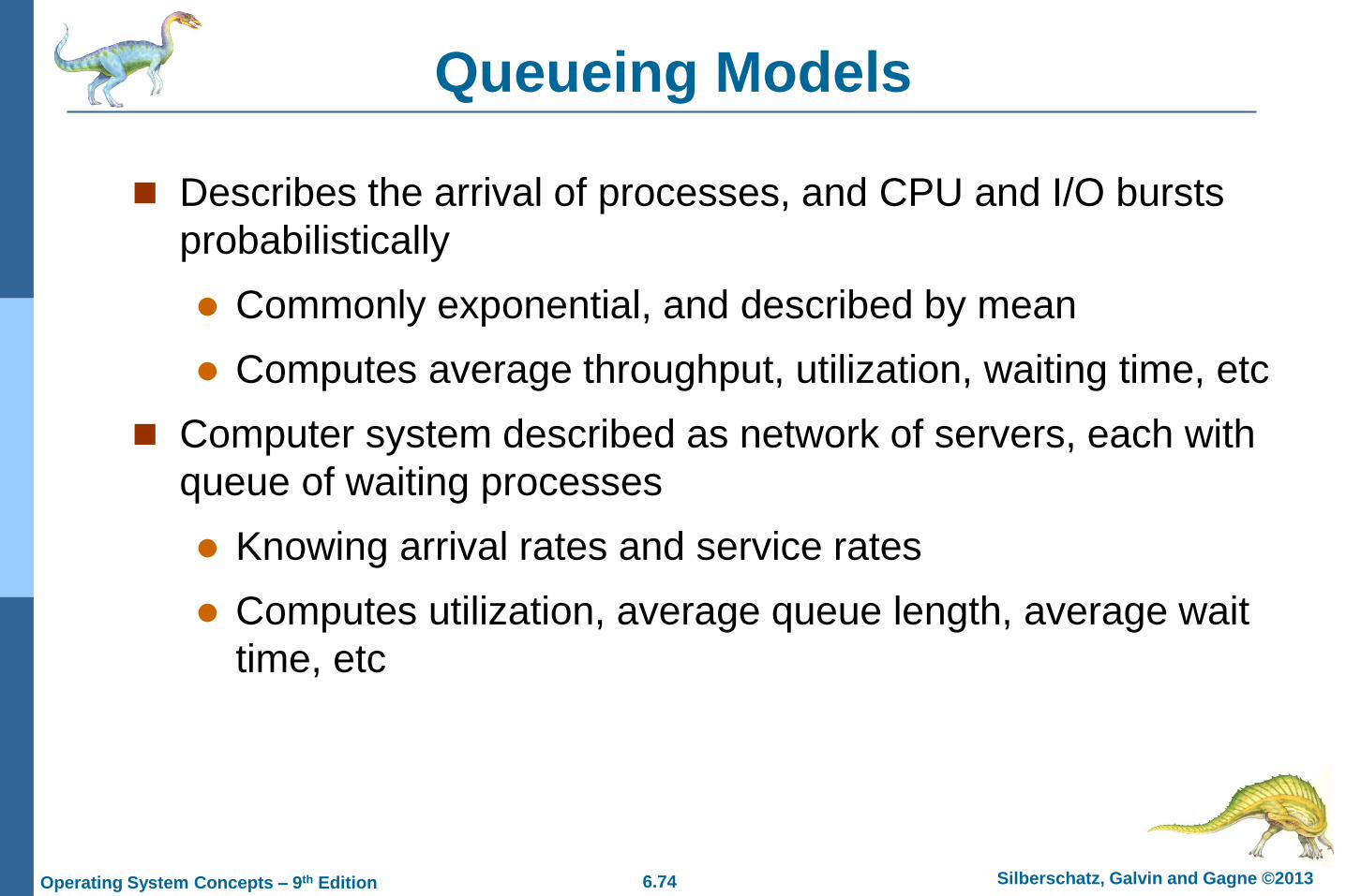
Queueing Models
Describes the arrival of processes, and CPU and I/O bursts
probabilistically
Commonly exponential, and described by mean
Computes average throughput, utilization, waiting time, etc
Computer system described as network of servers, each with
queue of waiting processes
Knowing arrival rates and service rates
Computes utilization, average queue length, average wait
time, etc
6.75 Silberschatz, Galvin and Gagne © 2013Operating System Concepts – 9th Edition
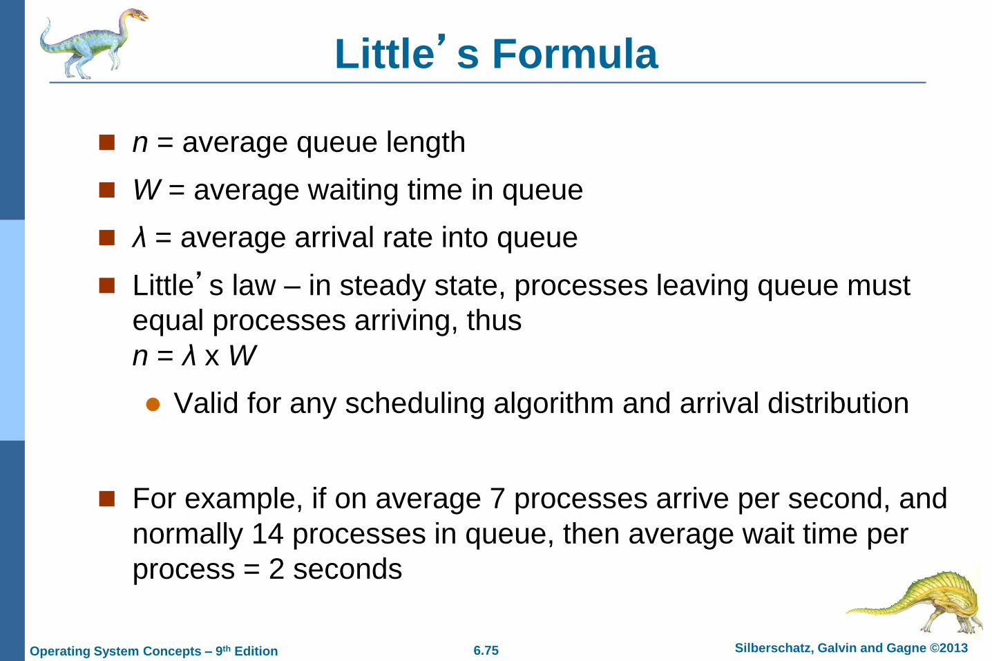
Little’s Formula
n = average queue length
W = average waiting time in queue
λ = average arrival rate into queue
Little’s law – in steady state, processes leaving queue must
equal processes arriving, thus
n = λ x W
Valid for any scheduling algorithm and arrival distribution
For example, if on average 7 processes arrive per second, and
normally 14 processes in queue, then average wait time per
process = 2 seconds
6.76 Silberschatz, Galvin and Gagne © 2013Operating System Concepts – 9th Edition
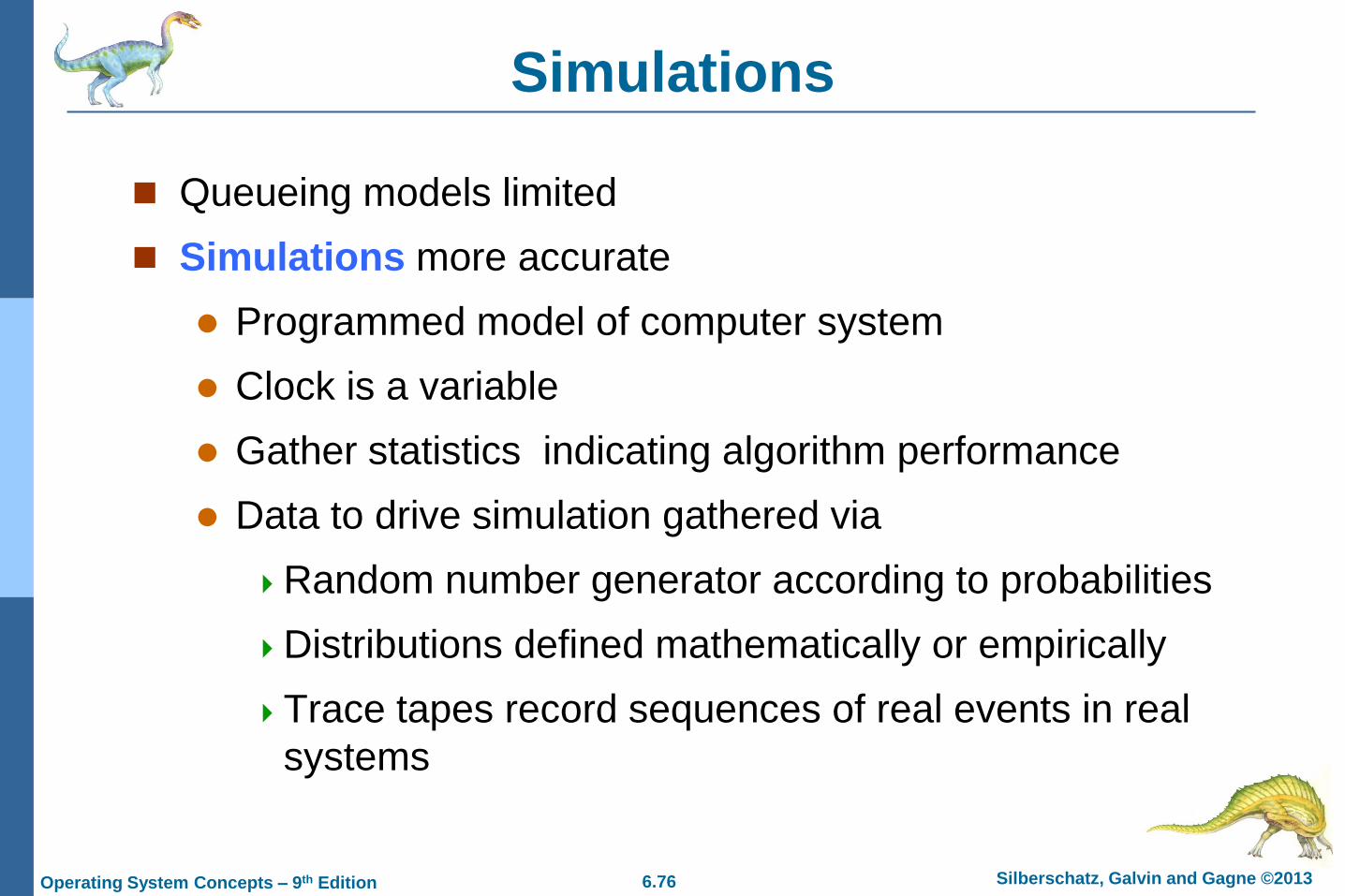
Simulations
Queueing models limited
Simulations more accurate
Programmed model of computer system
Clock is a variable
Gather statistics indicating algorithm performance
Data to drive simulation gathered via
Random number generator according to probabilities
Distributions defined mathematically or empirically
Trace tapes record sequences of real events in real
systems
6.77 Silberschatz, Galvin and Gagne © 2013Operating System Concepts – 9th Edition
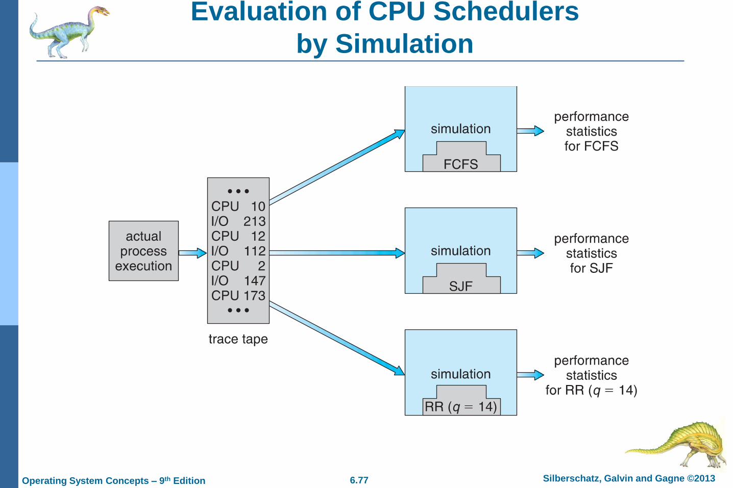
Evaluation of CPU Schedulers
by Simulation
6.78 Silberschatz, Galvin and Gagne © 2013Operating System Concepts – 9th Edition
Implementation
Even simulations have limited accuracy
Just implement new scheduler and test in real systems
High cost, high risk
Environments vary
Most flexible schedulers can be modified per-site or per-system
Or APIs to modify priorities
But again environments vary

6.79 Silberschatz, Galvin and Gagne © 2013Operating System Concepts – 9th Edition
Exercise (1/3)
6.80 Silberschatz, Galvin and Gagne © 2013Operating System Concepts – 9th Edition
Exercise (2/3)

6.81 Silberschatz, Galvin and Gagne © 2013Operating System Concepts – 9th Edition
Exercise (3/3)