Chapter 5: Monte Carlo Integration andVariance Reduction

Lecturer: Zhao Jianhua

Department of StatisticsYunnan University of Finance and Economics

Outline

5.2 Monte Carlo Integration5.2.1 Simple MC estimator5.2.2 Variance and Efficiency

5.3 Variance Reduction

5.4 Antithetic Variables

5.5 Control Variates5.5.1 Antithetic variate as control variate5.5.2 Several control variates5.5.3 Control variates and regression

5.6 Importance Sampling

5.7 Stratified Sampling

5.8 Stratified Importance Sampling

5.2 Monte Carlo (MC) Integration

I Monte Carlo (MC) integration is a statistical method basedon random sampling. MC methods were developed in the late1940s after World War II, but the idea of random sampling wasnot new.

I Let g(x) be a function and suppose that we want to compute∫ ba g(x) dx. Recall that if X is a r.v. with density f(x), then

the mathematical expectation of the r.v. Y = g(X) is

E[g(X)] =

∫ ∞−∞

g(x)f(x)dx.

I If a random sample is available from the dist. of X, an unbiasedestimator of E[g(X)] is the sample mean.

5.2.1 Simple MC estimator

I Consider the problem of estimating θ =∫ 10 g(x)d(x). IfX1, ..., Xm

is a random U(0, 1) sample, then

θ = gm(X) =1

m

∑m

i=1g(Xi).

converges to E[g(X)] = θ with probability 1, by the StrongLaw of Large Numbers (SLLN).

I The simple MC estimator of∫ 10 g(x)dx is gm(X).

Example 5.1 (Simple MC integration)

Compute a MC estimate of θ =∫ 10 e−xdx and compare the

estimate with the exact value.

m <- 10000; x <- runif(m); theta.hat <- mean(exp(-x))

print(theta.hat); print (1 - exp(-1))

[1] 0.6355289

[1] 0.6321206

The estimate is θ.= 0.6355 and θ = 1− e−1 .

= 0.6321.

To compute∫ ba g(t)dt, make a change of variables so that the limits

of integration are from 0 to 1. The linear transformation is y =(t− a)/(b− a) and dy = (1/(b− a)).∫ b

ag(t)dt =

∫ 1

0g(y(b− a) + a)(b− a)dy.

Alternately, replace the U(0, 1) density with any other density sup-ported on the interval between the limits of integration, e.g.,∫ b

ag(t)dt = (b− a)

∫ b

ag(t)

1

b− adt.

is b− a times the expected value of g(Y ), where Y has the uniformdensity on (a, b). The integral is therefore (b−a) times gm(X), theaverage value of g(·) over (a, b).

Example 5.2 (Simple MC integration, cont.)

Compute a MC estimate of θ =∫ 42 e−xdx. and compare the estimate

with the exact value of the integral.

m <- 10000

x <- runif(m, min=2, max=4)

theta.hat <- mean(exp(-x)) * 2

print(theta.hat)

print(exp(-2) - exp(-4))

[1] 0.1172158

[1] 0.1170196

The estimate is θ.= 0.1172 and θ = 1− e−1 .

= 0.1170.To summarize, the simple MC estimator of the integral θ =

∫ ba g(x)dx

is computed as follows.

1. Generate X1, ..., Xm, iid from U(a, b).

2. Compute g(X) = 1mg(Xi).

3. θ = (b− a)g(X).

Example 5.3 (MC integration, unbounded interval)

Use the MC approach to estimate the standard normal cdf

Φ(x) =

∫ x

−∞

1√2πe−t

2/2dt.

Since the integration cover an unbounded interval, we break thisproblem into two cases: x ≥ 0 and x < 0, and use the symmetry ofthe normal density to handle the second case.

I To estimate θ =∫ x0 e−t2/2dt for x > 0, we can generate ran-

dom U(0, x) numbers, but it would change the parameters ofuniform dist. for each different value.

We prefer an algorithm that always samples from U(0, 1) via achange of variables. Making the substitution y = t/x, we havedt = xdy and

θ =

∫ 1

0xe−(xy)

2/2dy.

Thus, θ = EY [xe−(xY )2/2], where r.v. Y has U(0, 1) dist.

Generate iid U(0, 1) random numbers u1, ..., um, and compute

θ = gm(u) =1

m

∑m

t=1xe−(uix)

2/2

Sample mean θ → E[θ] = θ as m→∞. If x > 0, estimate of Φ(x)is 0.5 + θ/

√2π. If x < 0, compute Φ(x) = 1− Φ(−x).

x<-seq(.1, 2.5, length =10); m <- 10000

u <- runif(m) c d f <- numeric(length(x))

for (i in 1: length(x)) {

g <- x[i] * exp(-(u * x[i])^2 / 2)

cdf[i] <- mean(g) / sqrt(2 * pi) + 0.5 }

Now the estimates θ for ten values of x are stored in the vector cdf.Compare the estimates with the value Φ(x) computed (numerically)by the pnorm function.

Phi <- pnorm(x); print(round(rbind(x, cdf , Phi), 3))

The MC estimates appear to be very close to the pnorm values (Theestimates will be worse in the extreme upper tail of the dist.)

[,1] [,2] [,3] [,4] [,5] [,6] [,7] [,8] [,9] [,10]

x 0.10 0.367 0.633 0.900 1.167 1.433 1.700 1.967 2.233 2.500

cdf 0.54 0.643 0.737 0.816 0.879 0.925 0.957 0.978 0.990 0.997

Phi 0.54 0.643 0.737 0.816 0.878 0.924 0.955 0.975 0.987 0.994

I It would have been simpler to generate random U(0, x) r.v. andskip the transformation. This is left as an exercise.

I In fact, the integrand is itself a density function, and we cangenerate r.v. from this density. This provides a more directapproach to estimating the integral.

Example 5.4 (Example 5.3, cont.)

Let I(·) be the indicator function, and Z ∼ N(0, 1). Then for anyconstant x we have E[I(Z ≤ x)] = P (Z ≤ x) = Φ(x).Generate a random sample z1, ..., zm from the standard normal dist.Then the sample mean

Φ(x) =1

m

∑m

i=1I(zi ≤ x)→ E[I(Z ≤ x)] = Φ(x).

x <- seq(.1, 2.5, length = 10)

m <- 10000; z <- rnorm(m)

dim(x) <- length(x)

p <- apply(x, MARGIN = 1,

FUN = function(x, z) {mean(z < x)}, z = z)

Compare the estimates in p to pnorm:[,1] [,2] [,3] [,4] [,5] [,6] [,7] [,8] [,9] [,10]

x 0.10 0.367 0.633 0.900 1.167 1.433 1.700 1.967 2.233 2.500

p 0.546 0.652 0.741 0.818 0.876 0.925 0.954 0.976 0.988 0.993

Phi 0.54 0.643 0.737 0.816 0.878 0.924 0.955 0.975 0.987 0.994

Compared with Example 5.3, better agreement with pnorm in theupper tail, but worse agreement near the center.

Summarizing, if f(x) is a probability density function supported ona set A (f(x) ≥ 0 for all x ∈ R and

∫A f(x) = 1), to estimate the

integral

θ =

∫Ag(x)f(x)dx,

generate a random sample x1, ..., xm from the dist. f(x), and com-pute the sample mean

θ =1

m

∑m

i=1g(xi).

Then with probability one, θ converges to E[θ] = θ as m→∞.

The standard error of θ = 1mΣm

i=1g(xi)

The variance of θ is σ2/m, where σ2 = V arf (g(X)). When thedist. of X is unknown we substitute for FX the empirical dist. Fmof the sample x1, ..., xm. The variance of θ can be estimated by

σ2

m=

1

m2

∑m

i=1[g(xi)− g(x)]2 (5.1)

1m

∑mi=1[g(xi) − g(x)]2 is the plug-in estimate of V ar(g(X)) and

the variance of U , where U is uniformly distributed on the set ofreplicates g(xi). The estimate of standard error of θ is

se(θ) =σ√m

=1

m{∑m

i=1[g(xi)− g(x)]2}1/2 (5.3)

The Central Limit Theorem (CLT) implies that (θ −E[θ])/√V arθ

converges in dist. to N(0, 1) as m→∞. Hence, θ is approximatelynormal with mean θ. The approximately normal dist. of θ can beapplied to put confidence limits or error bounds on the MC estimateof the integral, and check for convergence.

Example 5.5 (Error bounds for MC integration)

Estimate the variance of the estimator in Example 5.4, and constructapproximate 95% CI for estimates of Φ(2) and Φ(2.5).

x <- 2; m <- 10000; z <- rnorm(m)

g <- (z < x) #the indicator function

v <- mean((g - mean(g))^2) / m; cdf <- mean(g)

c(cdf , v); c(cdf - 1.96 * sqrt(v), cdf + 1.96 * sqrt(v))

[1] 9.772000e-01 2.228016e-06

[1] 0.9742744 0.9801256

The probability P (I(Z < x) = 1) is Φ(2) u 0.977. The varianceof g(X) is therefore (0.977)(1− 0.977)/10000 = 2.223e− 06. TheMC estimate 2.228e− 06 of variance is quite close to this value.For x = 2.5 the output is

[1] 9.94700e-01 5.27191e-07

[1] 0.9932769 0.9961231

The probability P (I(Z < x) = 1) is Φ(2.5) u 0.995. The M-C estimate 5.272e − 07 of variance is approximately equal to thetheoretical value (0.995)(1− 0.995)/10000 = 4.975e− 07.

5.2.2 Variance and Efficiency

If X ∼ U(a, b), then f(x) = 1b−a , a < x < b, and

θ =

∫ b

ag(x)dx = (b− a)

∫ b

ag(x)

1

b− adx = (b− a)E[g(X)].

Recall the sample-mean MC estimator of the integral θ:

1. Generate X1, ..., Xm, iid from U(a, b).

2. Compute g(X) = 1m

∑mi=1 g(Xi).

3. θ = (b− a)g(X).

Sample mean g(X) has expected value g(X) = θ/(b − a), andV ar(g(X)) = (1/m)V ar(g(X)). Therefore E[θ] = θ and

V ar(θ) = (b− a)2V ar(g(X)) =(b− a)2

mV ar(g(X)). (5.4)

By CLT, for large m, g(X) is approximately normally distributed,and therefore θ is approximately normally distributed with mean θand variance given by (5.4).

hit-or-miss approach

The hit-or-miss approach also uses a sample mean to estimate theintegral, but taken over a different sample and therefore this esti-mator has a different variance from formula (5.4).

Suppose f(x) is the density of a r.v. X. The hit-or-miss approachto estimating F (x) =

∫ x−∞ f(t)dt is as follows.

1. Generate a random sample X1, ..., Xm from the dist. of X.

2. For each observation Xi, compute

g(Xi) = I(Xi ≤ x) =

{1, Xi ≤ x;

0, Xi > x.

3. Compute F (x) = g(X) = 1mΣm

i=1I(Xi ≤ x).

Here, Y = g(X) ∼ Binomial(1, p), where p = P (X ≤ x) = F (x).The transformed sample Y1, ..., Ym are the outcomes of m i.i.d.

Bernoulli trials. The estimator F (x) is the sample proportion p =

y/m, where y is the total number of successes. Hence E[F (x)] =

p = F (x) and V ar(F (x)) = p(1− p)/m = F (x)(1− F (x))/m.

The variance of F (x) can be estimated by p(1− p)/m = F (x)(1−F (x))/m. The maximum variance occurs when F (x) = 1/2, so a

conservative estimate of the variance of F (x) is 1/(4m).

Efficiency

If θ1 and θ2 are two estimators for θ, then θ1 is more efficient (in astatistical sense) than θ2 if

V ar(θ1)

V ar(θ2)< 1.

If the variances of estimators θi are unknown, we can estimateefficiency by substituting a sample estimate of the variance foreach estimator.

Note that variance can always be reduced by increasing the numberof replicates, so computational efficiency is also relevant.

5.3 Variance Reduction

MC integration can be applied to estimate E[g(X)]. We now con-sider several approaches to reducing the variance in the sample meanestimator of θ = E[g(X)].

I If θ1 and θ2 are estimators of θ, and V ar(θ2) < V ar(θ1), thenthe percent reduction in variance achieved by using θ2:

100(V ar(θ1)− V ar(θ2)

V ar(θ1)).

MC approach computes g(X) for a large number m of replicatesfrom the dist. of g(X). When g(·) is a statistic, that is, an n-variate function g(X) = g(X1, ..., Xn), where X denotes the sampleelements.

Let X(j) ={X

(j)1 , ..., X(j)

n

}, j = 1, ...m

be iid from the dist. of X, and compute the corresponding replicates

Y (j) = g(X(1)n , ..., X(j)

n

), j = 1, ...m (5.5)

Then Y1, ..., Ym are i.i.d. with dist. of Y = g(X), and

E[Y ] = E

[1

m

∑m

j=1Yj

]= θ

Thus, the MC estimator θ = Y is unbiased for θ = E[Y ]. Thevariance of the MC estimator is

V ar(θ) = V arY =V arfg(X)

m.

Increasing m clearly reduces the variance of MC estimator. How-ever, a large increase in m is needed to get even a small improve-ment. To reduce the error from 0.01 to 0.0001, need approximately10000 times the number of replicates. If error is at most e andV arf (g(X)) = σ2, then m ≥ [σ2/e2] replicates are required.

I Thus, although variance can always be reduced by increasingthe number of MC replicates, the computational cost is high.

In the following, some approaches to reducing the variance of thistype of estimator are introduced.

5.4 Antithetic Variables

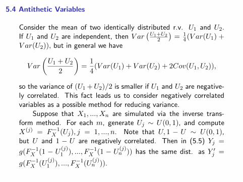
Consider the mean of two identically distributed r.v. U1 and U2.If U1 and U2 are independent, then V ar

(U1+U2

2

)= 1

4(V ar(U1) +V ar(U2)), but in general we have

V ar

(U1 + U2

2

)=

1

4(V ar(U1) + V ar(U2) + 2Cov(U1, U2)),

so the variance of (U1 +U2)/2 is smaller if U1 and U2 are negative-ly correlated. This fact leads us to consider negatively correlatedvariables as a possible method for reducing variance.

Suppose that X1, ..., Xn are simulated via the inverse trans-form method. For each m, generate Uj ∼ U(0, 1), and computeX(j) = F−1X (Uj), j = 1, ..., n. Note that U, 1 − U ∼ U(0, 1),but U and 1 − U are negatively correlated. Then in (5.5) Yj =

g(F−1X (1 − U (j)1 ), ..., F−1X (1 − U (j)

n )) has the same dist. as Y ′j =

g(F−1X (U(j)1 ), ..., F−1X (U

(j)n )).

Under what conditions are Yj and Y ′j negatively correlated? Belowit is shown that if the function g is monotone, the variables Yj andYj are negatively correlated.

Definition: n-variate monotone function(x1, ..., xn) ≤ (y1, ..., yn) if xj ≤ yj , j = 1, ..., n. An n-variatefunction g = g(X1, ..., Xn) is increasing (decreasing) if it isincreasing (decreasing) in its coordinates. That is, g is increasing(decreasing) if g(x1, ..., xn) ≤ (≥)g(y1, ..., yn) when (x1, ..., xn)≤ (≥)(y1, ..., yn). g is monotone if it is increasing/decreasing.

PROPOSITION 5.1 If (X1, ..., Xn) are independent, and f and gare increasing functions, then

E[f(X)g(X)] ≥ E[f(X)]E[g(X)] (5.6)

Proof. Assume that f and g are increasing functions. The proofis by induction on n. Suppose n = 1. Then (f(x) − f(y))(g(x) −g(y)) ≥ 0 for all x, y ∈ R. Hence E[(f(X)−f(Y ))(g(X)−g(Y ))] ≥0, and

E[f(X)g(X)] + E[f(Y )g(Y )] ≥ E[f(X)g(Y )] + E[f(Y )g(X)].

Here X and Y are iid, so

2E[f(X)g(X)] = E[f(X)g(X)] + E[f(Y )g(Y )]

≥ E[f(X)g(Y )] + E[f(Y )g(X)]

= 2E[f(X)]E[g(X)].

so the statement is true for n = 1. Suppose that the statement (5.6)is true for X ∈ Rn−1. Condition on Xn and apply the inductionhypothesis to obtain

E[f(X)g(X)][Xn = xn] ≥ E[f(X1, ..., Xn−1, xn)]E[g(X1, ...,

Xn−1, xn] = E[f((X) | Xn = xn)]E[g((X) |Xn = xn)].

or E[f(X)g(X) | Xn] ≥ E[f(X) | Xn]E[g(X) | Xn].

Now E[f(X) | Xn] and E[g(X) | Xn] are each increasing functionsof Xn, so applying the result for n = 1 and taking the expectedvalues of both sides

E[f(X)g(X)|Xn] ≥ E[E[f(X)|Xn]E[g(X)|Xn]

≥ E[f(X)]E[g(X)].

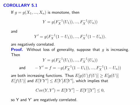
COROLLARY 5.1

If g = g(X1, ..., Xn) is monotone, then

Y = g(F−1X (U1)), ..., F−1X (Un))

andY ′ = g(F−1X (1− U1)), ..., F

−1X (1− Un)).

are negatively correlated.Proof. Without loss of generality, suppose that g is increasing.Then

Y = g(F−1X (U1)), ..., F−1X (Un))

and − Y ′ = f = −g(F−1X (1− U1)), ..., F−1X (1− Un))

are both increasing functions. Thus E[g(U)f(U)] ≥ E[g(U)]E[f(U)] and E[Y Y ′] ≤ E[Y ]E[Y ′], which implies that

Cov(Y, Y ′) = E[Y Y ′]− E[Y ][Y ′] ≤ 0,

so Y and Y’ are negatively correlated.

The antithetic variable approach is easy to apply. If m MC replicatesare required, generate m/2 replicates

Yj = g(F−1X (U(j)1 )), ..., F−1X (U (j)

n )) (5.7)

and the remaining m/2 replicates

Y ′j = g(F−1X (1− U (j)1 )), ..., F−1X (1− U (j)

n )) (5.8)

where U(j)i are iid U(0, 1) variables, i = 1, ..., n, j = 1, ...,m/2.

Then the antithetic estimator is

θ =1

m{Y1 + Y ′1 + Y2 + Y ′2 + ...+ Ym/2 + Y ′m/2}

=2

m

∑m/2

j=1

(Yj + Y ′J

2

)Thus nm/2 rather than nm uniform variates are required, and thevariance of the MC estimator is reduced by using antithetic variables.

Example 5.6 (Antithetic variables)

Refer to Example 5.3, estimation of the standard normal cdf

Φ(x) =

∫ x

−∞

1√2πe−t

2/2dt.

Now use antithetic variables, and find the approximate reduction instandard error. Now the target parameter is θ = EU [xe−(xU)2/2],where U has the U(0, 1) dist.

By restricting the simulation to the upper tail, the function g(·) ismonotone, so the hypothesis of Corollary 5.1 is satisfied. Generaterandom numbers u1, ..., um/2 ∼ U(0, 1) and compute half of thereplicates using

Yj = g(j)(u) = xe−(uj)x2/2, j = 1, ...,m/2

as before, but compute the remaining half of the replicates using

Y ′j = xe−(−(uj)x)2/2, j = 1, ...,m/2.

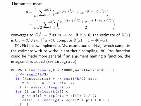
The sample mean

θ =1

m

∑m/2

j=1

(xe−(uj)x

2/2 + xe−((1−uj)x)2/2)

=1

m/2

∑m/2

j=1

(xe−(uj)x

2/2 + xe−((1−uj)x)2/2

2

)converges to E[θ] = θ as m → ∞. If x > 0, the estimate of Φ(x)is 0.5 + θ/

√2π. If x < 0 compute Φ(x) = 1− Φ(−x).

MC.Phi below implements MC estimation of Φ(x), which computethe estimate with or without antithetic sampling. MC.Phi functioncould be made more general if an argument naming a function, theintegrand, is added (see integrate).

MC.Phi <-function(x,R = 10000, antithetic=TRUE) {

u <- runif(R/2)

if (!antithetic) v <- runif(R/2) else

v <- 1 - u; u <- c(u, v)

cdf <- numeric(length(x))

for (i in 1: length(x)) {

g <- x[i] * exp(-(u * x[i])^2 / 2)

cdf[i] <- mean(g) / sqrt(2 * pi) + 0.5 }

cdf }

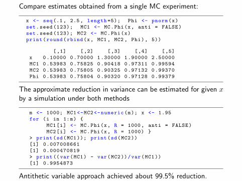
Compare estimates obtained from a single MC experiment:

x <- seq(.1, 2.5, length =5); Phi <- pnorm(x)

set.seed (123); MC1 <- MC.Phi(x, anti = FALSE)

set.seed (123); MC2 <- MC.Phi(x)

print(round(rbind(x, MC1 , MC2 , Phi), 5))

[,1] [,2] [,3] [,4] [,5]

x 0.10000 0.70000 1.30000 1.90000 2.50000

MC1 0.53983 0.75825 0.90418 0.97311 0.99594

MC2 0.53983 0.75805 0.90325 0.97132 0.99370

Phi 0.53983 0.75804 0.90320 0.97128 0.99379

The approximate reduction in variance can be estimated for given xby a simulation under both methods

m <- 1000; MC1 <-MC2 <-numeric(m); x <- 1.95

for (i in 1:m) {

MC1[i] <- MC.Phi(x, R = 1000, anti = FALSE)

MC2[i] <- MC.Phi(x, R = 1000) }

> print(sd(MC1)); print(sd(MC2))

[1] 0.007008661

[1] 0.000470819

> print ((var(MC1) - var(MC2))/var(MC1))

[1] 0.9954873

Antithetic variable approach achieved about 99.5% reduction.

5.5 Control Variates

Suppose that there is a function f , such that µ = E[f(X)] is known,and f(X) is correlated with g(X). Then for any constant c, θc =g(X) + c(f(X)−µ) is an unbiased estimator of θ = E[g(X)]. Thevariance

V ar(θc) = V ar(g(X)) + c2V ar(f(X)) + 2cCov(g(X), f(X))

is a quadratic function of c. It is minimized at c = c∗, where

c∗ = −Cov(g(X), f(X))

V ar(f(X))

and minimum variance is

V ar(θc∗) = V ar(g(X))− [Cov(g(X), f(X))]2

V ar(f(X)). (5.10)

f(X) is called a control variate for the estimator g(X). In (5.10),we see that V ar(g(X)) is reduced by

[Cov(g(X), f(X))]2

V ar(f(X)),

hence the percent reduction in variance is

100[Cov(g(X), f(X))]2

V ar(g(X))V ar(f(X))= 100[Cor(g(X), f(X))]2.

Thus, it is advantageous if f(X) and g(X) are strongly correlated.No reduction is possible in case f(X) and g(Y ) are uncorrelated.

To compute c∗, we need Cov(g(X), f(X)) and V ar(f(X)), butthey can be estimated from a preliminary MC experiment.

Example 5.7 (Control variate)

Apply the control variate approach to compute

θ = E[eU ] =

∫ 1

0eudu,

where U ∼ U(0, 1). θ = e− 1 = 1.718282 by integration. If thesimple MC approach is applied with m replicates, The variance ofthe estimator is V ar(g(U))/m, where V ar(g(U)) = V ar(eU ) =

E[eU ]− θ2 = e2−12 − (e− 1)2

.= 0.2420351.

A natural choice for a control variate is U ∼ U(0, 1). Then E[U ] =1/2, V ar(U) = 1/12, and Cov(eU , U) = 1 − (1/2)(e − 1)

.=

0.1408591. Hence

c∗ =−Cov(eU , U)

V ar(U)= −12 + 6(e− 1)

.= −1.690309.

Our controlled estimator is θc∗ = eU − 1.690309(U − 0.5). For mreplicates, mV ar(θc∗) is

V ar(eU )− −Cov(eU , U)

V ar(U)=e2 − 1

2− (e− 1)2 − 12

(1− e− 1

2

).= 0.2420356− 12(0.1408591)2 = 0.003940175.

The percent reduction in variance using the control variate comparedwith the simple MC estimate is 100(0.2429355−0.003940175/0.2429355) =98.3781%.

Empirically comparing the simple MC estimate with the control vari-ate approach

m <- 10000; a <- - 12 + 6 * (exp(1) - 1)

U <- runif(m); T1 <- exp(U) #simple MC

T2 <- exp(U) + a * (U - 1/2) #controlled

gives the following results

> mean(T1); mean(T2)

[1] 1.717834

[1] 1.718229

> (var(T1) - var(T2)) / var(T1)

[1] 0.9838606

illustrating that the percent reduction 98.3781% in variance derivedabove is approximately achieved in this simulation.

Example 5.8 (MC integration using control variates)

Use the method of control variates to estimate∫ 1

0

e−x

1 + x2dx

θ = E[g(X)] and g(X) = e−x/(1 + x2), where X ∼ U(0, 1).I We seek a function ‘close’ to g(x) with known expected value,

such that g(X) and f(X) are strongly correlated.

For example, the function f(x) = e−.5(1 + x2)−1 is close to g(x)on (0,1) and we can compute its expectation. If U ∼ U(0, 1), then

E[f(U)] = e−.5∫ 1

0

1

1 + u2du = e−.5arctan(1) = e−.5

π

4

Setting up a preliminary simulation to obtain an estimate of the con-stant c∗, we also obtain an estimate of Cor(g(U), f(U)) u 0.974.

f <- function(u) exp(-.5)/(1+u^2)

g <- function(u) exp(-u)/(1+u^2)

set.seed (510) #needed later

u <- runif (10000); B <- f(u); A <- g(u)

Estimates of c∗ and Cor(f(U), g(U)) are

> cor(A, B)

[1] 0.9740585

a <- -cov(A,B) / var(B) #est of c* >a

[1] -2.436228

Simulation results with and without the control variate follow.

m <- 100000; u <- runif(m)

T1 <- g(u); T2 <- T1 + a *(f(u) - exp(-.5)*pi/4)

> c(mean(T1), mean(T2))

[1] 0.5253543 0.5250021

> c(var(T1), var(T2))

[1] 0.060231423 0.003124814

> (var(T1) - var(T2)) / var(T1)

[1] 0.9481199

Here the approximate reduction in variance of g(X) compared withg(X)+c∗(f(X)−µ) is 95%. We will return to this problem to applyan other approach to variance reduction, the method of importancesampling.

5.5.1 Antithetic variate as control variate.

Antithetic variate is actually a special case of the control variateestimator. Notice that the control variate estimator is a linear com-bination of unbiased estimators of θ. In general, if θ1 and θ2 are anytwo unbiased estimators of θ, then for every constant c,

θc = cθ1 + (1− c)θ2

is also unbiased for θ. The variance of cθ1 + (1− c)θ2 is

V ar(θ2) + c2V ar(θ1 − θ2) + 2Cov(θ2, θ1 − θ2). (5.11)

For antithetic variates, θ1 and θ2 are identically distributed andCor(θ1, θ2) = −1. Then Cov(θ1, θ2) = −V ar(θ1), the variance

V ar(θc) = 4c2V ar(θ1)− 4cV ar(θ1) + V ar(θ1)

= (4c2 − 4c+ 1)V ar(θ1)

and the optimal constant is c∗ = 1/2. The control variate estimator

in this case is θc∗ = θ1+θ22 , which (for this particular choice of θ1

and θ2) is the antithetic variable estimator of θ.

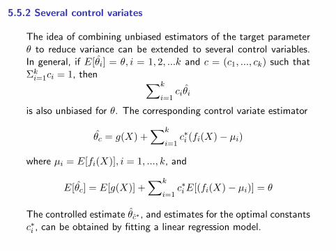
5.5.2 Several control variates

The idea of combining unbiased estimators of the target parameterθ to reduce variance can be extended to several control variables.In general, if E[θi] = θ, i = 1, 2, ...k and c = (c1, ..., ck) such thatΣki=1ci = 1, then ∑k

i=1ciθi

is also unbiased for θ. The corresponding control variate estimator

θc = g(X) +∑k

i=1c∗i (fi(X)− µi)

where µi = E[fi(X)], i = 1, ..., k, and

E[θc] = E[g(X)] +∑k

i=1c∗iE[(fi(X)− µi)] = θ

The controlled estimate θc∗ , and estimates for the optimal constantsc∗i , can be obtained by fitting a linear regression model.

5.5.3 Control variates and regression

I The duality between the control variate approach and simple lin-ear regression provides more insight into how the control variatereduces the variance in MC integration.

I In addition, we have a convenient method for estimating theoptimal constant c∗, the target parameter, the percent reduc-tion in variance, and the standard error of the estimator, all byfitting a simple linear regression model.

Suppose that (X1, Y1), ..., (Xn, Yn) is a random sample from a bi-variate dist. with mean (µX , µY ) and variances (σ2X , σ

2Y ). If there

is a linear relation X = β1Y + β0 + ε, and E[ε] = 0, then

E[X] = E[E[X | Y ]] = E[β0 + β1Y + ε] = β0 + β1µY .

Let us consider the bivariate sample (g(X1), f(X1)), ..., (g(Xn),f(Xn)). Now if g(X) replaces X and f(X) replaces Y , we haveg(X) = β0 + β1f(X) + ε, and

E[g(X)] = β0 + β1E[f(X)].

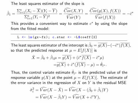
The least squares estimator of the slope is

β1 =Σni=1(Xi −X)(Yi − Y )

Σni=1(Yi − Y )2

=Cov(X,Y )

V ar(Y )=Cov(g(X), f(X))

V ar(f(X))= −c∗

This provides a convenient way to estimate c∗ by using the slopefrom the fitted model:

L <- lm(gx∼fx); c.star <- -L$coeff [2]

The least squares estimator of the intercept is β0 = g(X)−(−c∗)f(X),so that the predicted response at µ = E[f(X)] is

X = β0 + β1µ = g(X) + (c∗f(X)− c∗µ)

=g(X) + c∗(f(X)− µ) = θc∗ .

Thus, the control variate estimate θc∗ is the predicted value of theresponse variable g(X) at the point µ = E[f(X)]. The estimate ofthe error variance in the regression of X on Y is the residual MSE

σ2ε = V ar(X − X) = V ar(X − (β0 + β1)Y )

= V ar(X − β1Y ) = V ar(X + c∗Y ),

The estimate of variance of the control variate estimator is

V ar(g(X)) + c∗(f(X)− µ) =V ar(g(X) + c∗(f(X)− µ))

n

=V ar(g(X) + c∗(f(X)))

n=σ2εn

Thus, the estimated standard error of the control variate estimateis easily computed using R by applying the summary method to thelm object from the fitted regression model, for example using

se.hat <- summary(L)$sigma

to extract the value of σε =√MSE.

Finally, recall that the proportion of reduction in variance for thecontrol variate is [Cor(g(X), f(X))]2. In the simple linear regressionmodel, the coefficient of determination is same number (R2), whichis the proportion of total variation in g(X) about its mean explainedby f(X).

Example 5.9 (Control variate and regression)

Returning to Example 5.8, let us repeat the estimation by fitting aregression model. In this problem,

g(x) =

∫ 1

0

e−x

1 + x2dx

and the control variate is

f(x) = e−.5(1 + x2)−1, 0 < x < 1.

with µ = E[f(X)] = e−.5π/4. To estimate the constant c∗,

set.seed (510)

u <- runif (10000)

f <- exp(-.5)/(1+u^2)

g <- exp(-u)/(1+u^2)

c.star <- - lm(g∼f)$coeff [2] # beta [1]

mu <- exp(-.5)*pi/4

> c.star

f

-2.436228

Used the same seed as in Example 5.8 and obtained the sameestimate for c∗. Now θc∗ is the predicted response at the pointµ = 0.4763681, so

u <- runif (10000); f <- exp(-.5)/(1+u^2)

g <- exp(-u)/(1+u^2); L <- lm(g∼f)

theta.hat <- sum(L$coeff * c(1, mu)) #pred. value at mu

Estimate θ, residual MSE and the proportion of reduction in variance(R-squared) agree with the estimates obtained in Example 5.8.

> c(theta.hat ,summary(L)$sigma^2,summary(L)$r.squared)[1] 0.5253113 0.003117644 0.9484514

In case several control variates are used, one can estimate the model

X = β0 +∑k

i=1βiYi + ε

to estimate the optimal constants c∗ = (c∗1, ..., c∗k). Then −c∗ =

(β1, ..., βk) and the estimate is the predicted response X at the pointµ = (µ1, ..., µk). The estimated variance of the controlled estimatoris again σ2ε/n = MSE/n, where n the number of replicates.

5.6 Importance Sampling (IS)

The average value of a function g(x) over an interval (a, b) is1b−a

∫ ba g(x)dx. Here a uniform weight function is applied over the

entire interval (a, b). If X ∼ U(a, b), then

E[g(X)] =

∫ b

ag(x)

1

b− adx =

1

b− a

∫ b

ag(x)dx, (5.12)

The simple MC method generates a large number of replicatesX1, ...,Xm ∼ U [a, b] and estimates

∫ ba g(x)dx by the sample mean

b− am

∑m

i=1g(Xi),

which converges to∫ ba g(x)dx with probability 1 by SLLN. However,

this method has two limitations:

I it does not apply to unbounded intervals.

I it can be inefficient to draw samples uniformly across the inter-val if the function g(x) is not very uniform.

However, once we view the integration problem as an expected valueproblem (5.12), it seems reasonable to consider other weight func-tions (other densities) than uniform. This leads us to a generalmethod called importance sampling (IS).

Suppose X is a r.v. with density f(x), such that f(x) > 0 onthe set x : g(x) > 0. Let Y be r.v. g(X)/f(X). Then∫

g(x)dx =

∫g(x)

f(x)f(x)dx = E[Y ].

Estimate E[Y ] by simple MC integration by computing the average

1

m

∑m

i=1Yi =

1

m

∑m

i=1

g(Xi)

f(Xi),

where X1, ..., Xm are generated from the dist. with density f(x).f(x) is called the importance function.

In IS method, the variance of the estimator based on Y =g(X)/f(X) is V ar(Y )/m, so the variance of Y is small if Y isnearly constant (f(·) is ‘close’ to g(x)). Also, the variable withdensity f(·) should be reasonably easy to simulate.

I In Example 5.5, random normals are generated to compute theMC estimate of the standard normal cdf, Φ(2) = P (X ≤ 2).

I In the naive MC approach, estimates in the tails of the dist.are less precise.

Intuitively, we might expect a more precise estimate if the simulateddist. is not uniform, This method is called importance sampling (IS).Its advantage is that the IS dist. can be chosen so that variance ofthe MC estimator is reduced.

Suppose that f(x) is a density supported on a set A. If Φ(x) > 0on A, the integral θ =

∫A g(x)f(x)dx, can be written

θ =

∫Ag(x)

f(x)

φ(x)φ(x)dx.

If φ(x) is a density on A, an estimator of θ = Eφ[g(x)f(x)/φ(x)] is

θ =1

n

∑m

i=1g(Xi)

f(Xi)

φ(Xi),

Example 5.10 (Choice of the importance function)

Several possible choices of importance functions to estimate∫ 1

0

e−x

1 + x2dx

by IS method are compared. The candidates are

f0(x) = 1, 0 < x < 1, f1(x) = e−x, 0 < x <∞,f2(x) = (1 + x2)−1/π, −∞ < x <∞,f3(x) = e−x/(1− e−1), 0 < x < 1,

f4(x) = 4(1 + x2)−1/π, 0 < x < 1.

The integrand is

g(x) =

{e−x/(1 + x2), if 0 < x < 1;

0, otherwise.

While all five candidates are positive on the set 0 < x < 1 whereg(x) > 0, f1 and f2 have larger ranges and many of the simulatedvalues will contribute zeros to the sum, which is inefficient.

All of these dist. are easy to simulate; f2 is standard Cauchy ort(v = 1). The densities are plotted on (0, 1) for easy comparison.The function that corresponds to the most nearly constant ratiog(x)/f(x) appears to be f3, which can be seen more clearly in Fig.5.1(b). From the graphs, we might prefer f3 for the smallest variance(Code to display Fig.5.1(a) and (b) is given on page 152).

0.0 0.2 0.4 0.6 0.8 1.0

0.0

0.5

1.0

1.5

2.0

x

g

0

1

2

3

4

(a)

0.0 0.2 0.4 0.6 0.8 1.0

0.0

0.5

1.0

1.5

2.0

2.5

3.0

x

0

1

2

3

4

(b)

Fig. 5.1: Importance functions in Example 5.10: f0, ..., f4 (lines 0:4) with

g(x) in (a) and the ratios g(x)/f(x) in (b).

m <- 10000; theta.hat <- se <- numeric (5)

g <- function(x) {

exp(-x - log (1+x^2)) * (x > 0) * (x < 1) }

x <- runif(m) #using f0

fg <- g(x); theta.hat [1] <- mean(fg); se[1] <- sd(fg)

x <- rexp(m, 1) #using f1

fg<-g(x)/exp(-x); theta.hat [2] <-mean(fg); se[2] <-sd(fg)

x <- rcauchy(m) #using f2

i <- c(which(x > 1), which(x < 0))

x[i] <- 2 #to catch overflow errors in g(x)

fg<-g(x)/dcauchy(x); theta.hat [3] <-mean(fg); se[3] <-sd(fg)

u <- runif(m) #f3 , inverse transform method

x <- - log(1 - u * (1 - exp( -1)))

fg=g(x)/(exp(-x)/(1-exp ( -1)));

theta.hat [4]= mean(fg);se[4]=sd(fg)

u <- runif(m) #f4 , inverse transform method

x <- tan(pi*u/4); fg<-g(x)/(4/((1 + x^2)*pi))

theta.hat[5] <- mean(fg); se[5] <- sd(fg)

Five Estimates of∫ 10 g(x)dx and their standard errors se are

> rbind(theta.hat , se)[,1] [,2] [,3] [,4] [,5]

theta.hat 0.5241140 0.5313584 0.5461507 0.52506988 0.5260492

se 0.2436559 0.4181264 0.9661300 0.09658794 0.1427685

f3 and possibly f4 produce smallest variance among five candidates,while f2 produces the highest variance. The standard MC estimatewithout IS has se

.= 0.244(f0 = 1).

f2 is supported on (−∞,∞), while g(x) is evaluated on (0,1).There are a very large number of zeros (about 75%) produced inthe ratio g(x)/f(x), and all other values far from 0, resulting in alarge variance. Summary statistics for g(x)/f2(x) confirm this.

Min. 1st Qu. Median Mean 3rd Qu. Max.

0.0000 0.0000 0.0000 0.5173 0.0000 3.1380

For f1 there is a similar inefficiency, as f1 is supported on (0,∞).Choice of importance function: f is supported on exactly the setwhere g(x) > 0, and the ratio g(x)/f(x) is nearly constant.

Variance in Importance Sampling (IS)

If φ(x) is the IS dist. (envelope), f(x) = 1 on A, and X has pdfφ(x) supported on A, then

θ =

∫Ag(x)dx =

∫A

g(x)

φ(x)φ(x)dx = E

[g(X)

φ(X)

].

If X1, ..., Xn is a random sample from the dist. of X, the estima-tor θ = g(X) = 1

n

∑ni=1

g(Xi)φ(Xi)

. Thus IS method is a sample-meanmethod, and

V ar(θ) = E[θ2]− (E[θ])2 =

∫A

g2(x)

φ(x)ds− θ2

The dist. of X can be chosen to reduce the variance of the sam-ple mean estimator. The minimum variance

( ∫A |g(x)|dx

)2 − θ2 is

obtained when φ(x) = |g(x)|∫A |g(x)|dx

. Unfortunately, it is unlikely that

the value of∫A |g(x)|dx is available. Although it may be difficult to

choose φ(x) to attain minimum variance, variance maybe ‘close to’optimal if φ(x) is ‘close to’ |g(x)| on A.

5.7 Stratified Sampling

Stratified sampling aims to reduce the variance of the estimator bydividing the interval into strata and estimating the integral on eachof the stratum with smaller variance.

I Linearity of the integral operator and SLLN imply that the sumof these estimates converges to

∫g(x)dx with probability 1.

The number of replicates m and mj to be drawn from each of kstrata are fixed so that m = m1 + +mk, with the goal that

V ar(θk(m1 + · · ·+mk)) < V ar(θ),

where θk(m1 + · · · + mk) is the stratified estimator and θ is thestandard MC estimator based on m = m1 + · · ·+mk replicates.

Example 5.11 (Example 5.10, cont.)

In Fig. 5.1(a), it is clear that g(x) is not constant on (0,1). Dividethe interval into, say, four subintervals, and compute a MC estimateof the integral on each subinterval using 1/4 of the total number ofreplicates. Then combine these four estimates to obtain the estimateof∫ 10 e−x(1 + x2)−1dx.

Results shows stratification has improved variance by a factor ofabout 10. For integrands that are monotone functions, stratificationsimilar to Exp.5.11 should be an effective way to reduce variance.

M <- 20 #number of replicates

T2 <- numeric (4)

estimates <- matrix(0, 10, 2)

g <- function(x) {

exp(-x - log(1+x^2)) * (x > 0) * (x < 1) }

for (i in 1:10) {

estimates[i, 1] <- mean(g(runif(M)))

T2[1] <- mean(g(runif(M/4, 0, .25)))

T2[2] <- mean(g(runif(M/4, .25, .5)))

T2[3] <- mean(g(runif(M/4, .5, .75)))

T2[4] <- mean(g(runif(M/4, .75, 1)))

estimates[i, 2] <- mean(T2) }

> estimates

[,1] [,2]

[1,] 0.6281555 0.5191537

[2,] 0.5105975 0.5265614

[3,] 0.4625555 0.5448566

[4,] 0.4999053 0.5151490

[5,] 0.4984972 0.5249923

[6,] 0.4886690 0.5179625

[7,] 0.5151231 0.5246307

[8,] 0.5503624 0.5171037

[9,] 0.5586109 0.5463568

[10,] 0.4831167 0.5548007

> apply(estimates , 2, mean)

[1] 0.5195593 0.5291568

> apply(estimates , 2, var)

[1] 0.0023031762 0.0002012629

PROPOSITION 5.2 Denote the standard MC estimator with Mreplicates by θM , and let

θS =1

k

∑k

j=1θj

denote the stratified estimator with equal size m = M/k strata.Denote the mean and variance of g(U) on stratum j by θj and σ2j ,

respectively. Then V ar(θM ) ≥ V ar(θS).

Proof. By independence of θj ’s,

V ar(θS) = V ar

(1

k

∑k

j=1θj

)=

1

k2

∑k

j=1

σ2jm

=1

MK

∑k

j−1σ2j .

Now, if J is the randomly selected stratum, it is selected with uni-form probability 1/k, and applying the conditional variance formula

V ar(θS) =V ar(g(U))

M=

1

M(V ar(E[g(U |J)])) + E[V ar(g(U |J))]

=1

M(V ar(θj) + E[σ2j ]) =

1

M

(V ar(θj) +

1

k

∑k

j=1σ2j)

=1

M(V ar(θj) + V ar(θS)) ≥ V ar(θS).

The inequality is strict except in the case where all the strata haveidentical means. A similar proof can be applied in the general casewhen the strata have unequal probabilities.

From the above inequality it is clear that the reduction in varianceis larger when the means of the strata are widely dispersed.

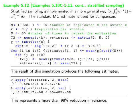
Example 5.12 (Examples 5.10C-5.11, cont., stratified sampling)

Stratified sampling is implemented in a more general way for∫ 10 e−x(1+

x2)−1dx. The standard MC estimate is used for comparison.

M<-10000; k <- 10 #number of replicates M and strata k

r <- M / k #replicates per stratum

N <- 50 #number of times to repeat the estimation

T2 <- numeric(k); estimates <- matrix(0, N, 2)

g <- function(x) {

exp(-x - log (1+x^2)) * (x > 0) * (x < 1) }

for (i in 1:N) {estimates[i, 1] <- mean(g(runif(M)))

for (j in 1:k)

T2[j] <- mean(g(runif(M/k, (j-1)/k, j/k)))

estimates[i, 2] <- mean(T2) }

The result of this simulation produces the following estimates.

> apply(estimates , 2, mean)

[1] 0.5251321 0.5247715

> apply(estimates , 2, var) [

1] 6.188117e-06 6.504485e-08

This represents a more than 98% reduction in variance.

5.8 Stratified Importance Sampling (IS)

Stratified IS is a modification to IS. Choose a suitable importancefunction f . Suppose that X is generated with density f and cdfF using the probability integral transformation. If M replicates aregenerated, the IS estimate of θ has variance σ2/M , where σ2 =V ar(g(X)/f(X)). For stratified IS estimate,

I divide the real line into k intervals Ij = {x : aj−1 ≤ x < aj}with endpoints a0 = −∞, aj = F−1(j/k), j = 1, ..., k− 1, andak =∞.

I The real line is divided into intervals corresponding to equalareas 1/k under the density f(x). The interior endpoints arethe percentiles or quantiles. On each subinterval define gj(x) =g(x) if x ∈ Ij and gj(x) = 0 otherwise.

We now have k parameters to estimate, θj =∫ ajaj−1

gj(x)dx, j =

1, ...k and θ = θ1 + ... + θk. The conditional densities provide theimportance functions on each subinterval.

On each subinterval Ij , conditional density fj of X is

fj(x) = fX|Ij =f(x, aj−1 ≤ x ≤ aj)P (aj−1 ≤ x < aj)

=f(x)

1/k= kf(x), aj−1 ≤ x < aj ,

Let σ2j = V ar(gj(X)/fj(X)). For each j = 1, ..., k, simulate an

importance sample size m, compute IS estimator θj on the jth subin-

terval, and compute θSI = 1kΣk

j=1θj . By independence of θ1, ..., θk,

V ar(θSI) = V ar(∑k

j=1θj)

=∑k

j=1

σ2jm

=1

m

∑k

j=1σ2j .

Denote the IS estimator by θI . We need to check that V ar(θSI)is smaller than the variance without stratification. The variance isreduced by stratification if

σ2

M>

1

m

∑k

j=1σ2j =

k

M

∑k

j=1σ2j ⇒ σ2 = k

∑k

j=1σ2j > 0.

Thus, we need to prove the following.

PROPOSITION 5.3 Suppose M = mk is the number of replicatesfor IS and stratified IS estimator θI and θSI , with estimates θI for θjon the individual strata, each with m replicates. If V ar(θI) = σ2/Mand V ar(θI) = σ2j /m, j = 1, ..., k, then

σ2 − k∑k

j−1σ2j ≥ 0, (5.13)

with equality if and only if θ1 = · · · = θk. Hence a stratificationreduces the variance except when g(x) is constant.

Proof.Consider a two-stage experiment. First a number J is drawnat random from the integers 1 to k. After observing J = j, arandom variable X∗ is generated from the density fj and

Y ∗ =gj(X)

fj(X)=

gj(X∗)

kfj(X∗).

To compute the variance of Y ∗, apply conditional variance formula

V ar(Y ∗) = E[V ar(Y ∗|J)] + V ar(E[Y ∗|J ]) (5.14)

Here E[V ar(Y ∗|J)] =∑k

j=1σ2jP (J = j) =

1

k

∑k

j=1σ2j ,

and V ar(Y ∗|J) = V ar(θJ). Thus in (5.14) we have V ar(Y ∗) =1k

∑kj=1 σ

2j + V ar(θJ). On the other hand,

k2V ar(Y ∗) = k2E[V ar(Y ∗|J) + k2V ar(E[Y ∗|J ]).

andσ2 = V ar(Y ) = V ar(kY ∗) = k2V ar(Y ∗)

which imply that

σ2 = k2V ar(Y ∗) = k2(1

k

∑k

j=1σ2j+V ar(θJ)

)= k

∑k

j=1σ2j+k

2V ar(θJ).

Therefore, σ2 − k∑k

j−1σ2j = k2V ar(θJ) ≥ 0,

and equality holds if and only if θ1 = · · · = θk.

Example 5.13 (Example 5.10, cont.)

I In Exp. 5.10, our best result was obtained with importancefunction f3(x) = e−x/(1 − e−1), 0 < x < 1. From 10000replicates we obtained the estimate θ = 0.5257801 and anestimated standard error 0.0970314.

I Now divide the interval (0,1) into five subintervals, (j/5, (j +1)/5), j = 0, 1, ..., 4. Then on the jth subinterval variables aregenerated from the density

5e−x

1− e−1,

j − 1

5< x <

j

5.

The implementation is left as an exercise.