chapter 4 : time response - unimap portalportal.unimap.edu.my/portal/page/portal30/lecture... ·...

UNIVERSITI MALAYSIA

PERLIS(UniMAP) LECTURE NOTE

SSCCHHOOOOLL OOFF MMEECCHHAATTRROONNIICCSS EENNGGIINNEEEERRIINNGG

ENT385: CONTROL ENGINEERING

2014/2015 – Sem I/ II

CHAPTER 4 : TIME –DOMAIN ANALYSIS

4.1 POLES, ZEROS, AND SYSTEM RESPONSE

The output response of a system is the sum of two responses: the forced response and the natural

response.

Forced response is also called the steady state error or particular solution.

Natural response is called the homogenous solution.

Poles of a Transfer Function

Value of Laplace transform variable, s that cause the transfer function to be come infinite; or

Any roots of the denominator of transfer function that are common to roots of numerator.

Zeros of a Transfer Function

Value of Laplace Transform variable, s that cause to become zero; or

Any roots of numerator of the transfer function that common to roots of denominator.

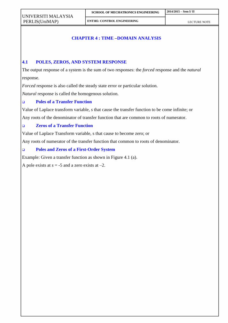
Poles and Zeros of a First-Order System

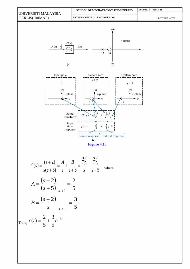
Example: Given a transfer function as shown in Figure 4.1 (a).

A pole exists at s = -5 and a zero exists at –2.

UNIVERSITI MALAYSIA




2014/2015 – Sem I/ II

Figure 4.1:

5

53

52

5)5(

)2()(

sss

B

s

A

ss

ssC

where,

5

2

5

2

0

ss

sA

5

3

2

5

ss

sB

Thus, tetc 5

5

3

5

2)(

UNIVERSITI MALAYSIA




2014/2015 – Sem I/ II

From the development summarized in Figure 4.1(c), we draw the following conclusions:

1. A pole of the input function generates the form of the forced response (i.e., the pole at the

origin generated a step function at the output).

2. A pole of the transfer function generates the form of the natural response (i.e., the pole at

–5 generated e-5t

).

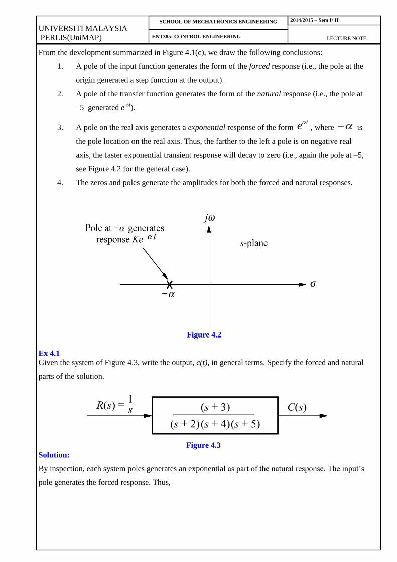
3. A pole on the real axis generates a exponential response of the form te , where is

the pole location on the real axis. Thus, the farther to the left a pole is on negative real

axis, the faster exponential transient response will decay to zero (i.e., again the pole at –5,

see Figure 4.2 for the general case).

4. The zeros and poles generate the amplitudes for both the forced and natural responses.

Figure 4.2

Ex 4.1

Given the system of Figure 4.3, write the output, c(t), in general terms. Specify the forced and natural

parts of the solution.

Figure 4.3

Solution:

By inspection, each system poles generates an exponential as part of the natural response. The input’s

pole generates the forced response. Thus,

UNIVERSITI MALAYSIA




2014/2015 – Sem I/ II

Response Natural ResponseForced

4321

)5()4()2( )(

s

K

s

K

s

K

s

KsC

Taking inverse transform, we get


5

4

4

3

2

21

)( ttt eKeKeKKtc

Ex 4.2

A system has a transfer function, )10)(8)(7)(1(

)6)(4(10)(

ssss

sssG

. Write, by

inspection, the output, c(t), in general terms if the input is a unit step.


)10()8()7()1( )(

s

E

s

D

s

C

s

B

s

AsC


1087

)( tttt EeDeCeBeAtc

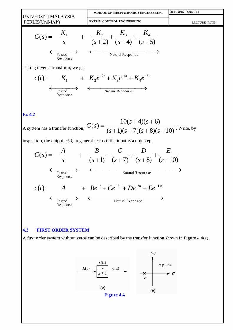
4.2 FIRST ORDER SYSTEM

A first order system without zeros can be described by the transfer function shown in Figure 4.4(a).

Figure 4.4

UNIVERSITI MALAYSIA




2014/2015 – Sem I/ II

If the input is a unit step , where s

sR1

)(

The Laplace transform of the step response is C(s), where

)()()()(

ass

asRsGsC

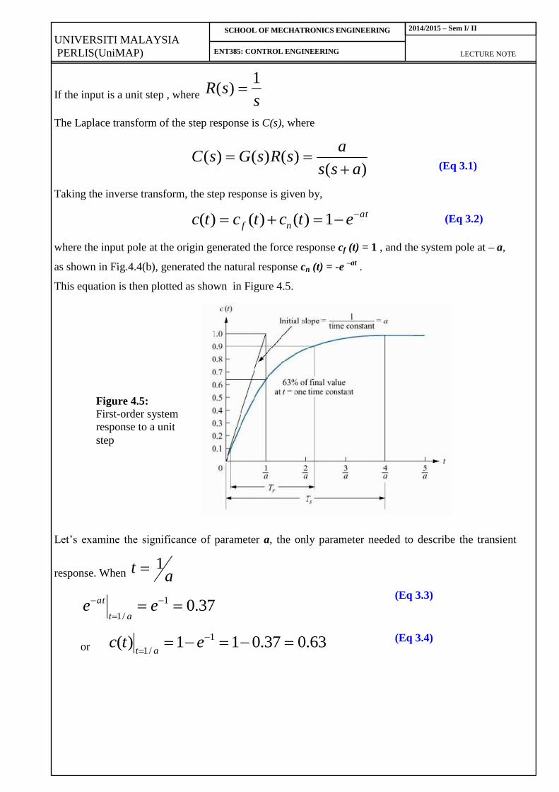
Taking the inverse transform, the step response is given by,

at

nf etctctc 1)()()(

where the input pole at the origin generated the force response cf (t) = 1 , and the system pole at – a,

as shown in Fig.4.4(b), generated the natural response cn (t) = -e –at

.

This equation is then plotted as shown in Figure 4.5.

Let’s examine the significance of parameter a, the only parameter needed to describe the transient

response. When at 1

37.01

/1

eeat

at

or 63.037.011)( 1

/1

etc

at

(Eq 3.1)

(Eq 3.2)

(Eq 3.3)

(Eq 3.4)

Figure 4.5:

First-order system

response to a unit

step

UNIVERSITI MALAYSIA




2014/2015 – Sem I/ II

Now we define three transient response performance specifications for first-order system.

Time Constant

1/a is the time constant of the response.

From Eq.(4.3), the time constant can be described as the time for e-at

to decay to 37% of its initial

value.

Alternately, from Eq.(4.4), the time constant is the time it takes for the step response to rise to 63% of

its final value (Fig.4.5).

The reciprocal of the time constant has the units (1/seconds), or frequency.

We can call the parameter a the exponential frequency.

Since, the derivative of e-at

is –a when t = 0, a is the initial rate of change of the exponential at t = 0.

Thus, the time constant can be considered a transient response specification for a first-order system,

since it is related to the speed at which the system responds to a step input.

The time constant can also be evaluated from the pole plot (Fig.4.4(b)).

Since, the pole of the transfer function is at –a, we can say the pole is located at the reciprocal of the

time constant, and the farther the pole from the imaginary axis, the faster the transient response.

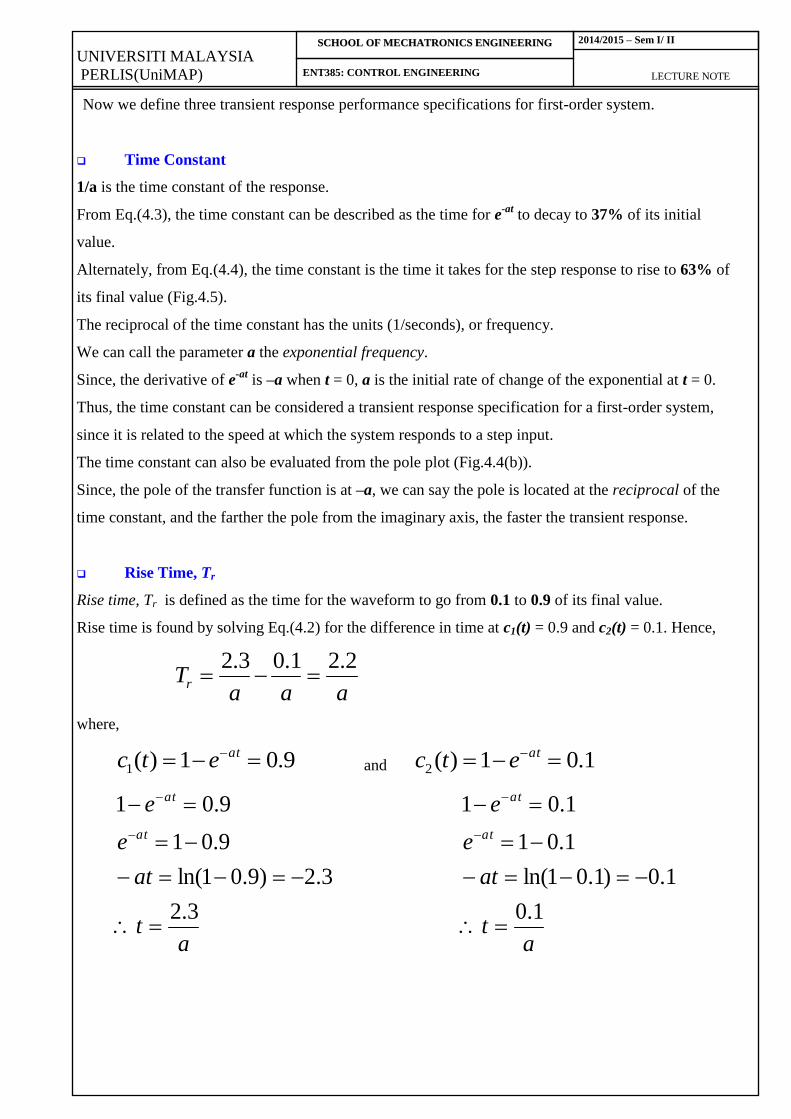
Rise Time, Tr

Rise time, Tr is defined as the time for the waveform to go from 0.1 to 0.9 of its final value.

Rise time is found by solving Eq.(4.2) for the difference in time at c1(t) = 0.9 and c2(t) = 0.1. Hence,

aaaTr

2.21.03.2

where,

9.01)(1 atetc and 1.01)(2 atetc

at

at

e

e

at

at

3.2

3.2)9.01ln(

9.01

9.01

at

at

e

e

at

at

1.0

1.0)1.01ln(

1.01

1.01

UNIVERSITI MALAYSIA




2014/2015 – Sem I/ II

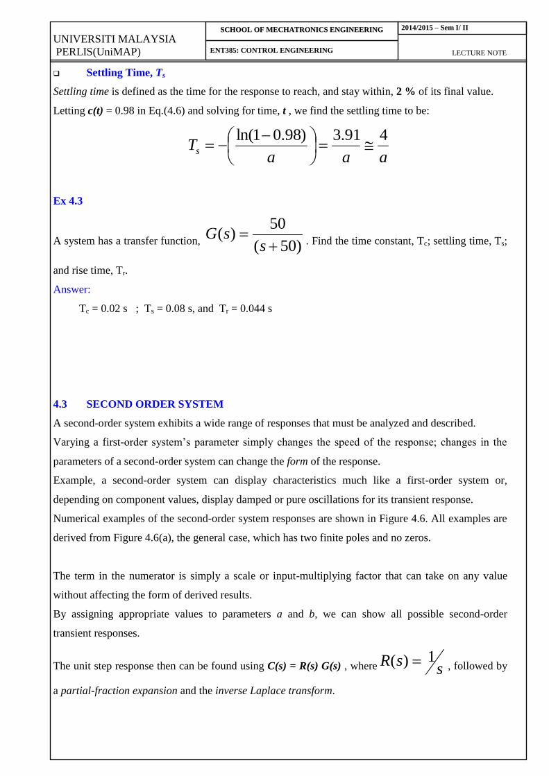
Settling Time, Ts

Settling time is defined as the time for the response to reach, and stay within, 2 % of its final value.

Letting c(t) = 0.98 in Eq.(4.6) and solving for time, t , we find the settling time to be:

aaaTs

491.3)98.01ln(

Ex 4.3

A system has a transfer function, )50(

50)(

ssG

. Find the time constant, Tc; settling time, Ts;

and rise time, Tr.

Answer:

Tc = 0.02 s ; Ts = 0.08 s, and Tr = 0.044 s

4.3 SECOND ORDER SYSTEM

A second-order system exhibits a wide range of responses that must be analyzed and described.

Varying a first-order system’s parameter simply changes the speed of the response; changes in the

parameters of a second-order system can change the form of the response.

Example, a second-order system can display characteristics much like a first-order system or,

depending on component values, display damped or pure oscillations for its transient response.

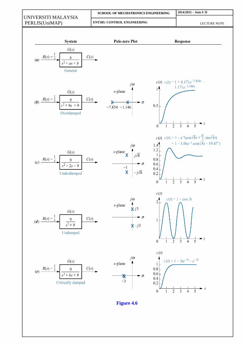
Numerical examples of the second-order system responses are shown in Figure 4.6. All examples are

derived from Figure 4.6(a), the general case, which has two finite poles and no zeros.

The term in the numerator is simply a scale or input-multiplying factor that can take on any value

without affecting the form of derived results.

By assigning appropriate values to parameters a and b, we can show all possible second-order

transient responses.

The unit step response then can be found using C(s) = R(s) G(s) , where ssR 1)( , followed by

a partial-fraction expansion and the inverse Laplace transform.

UNIVERSITI MALAYSIA




2014/2015 – Sem I/ II

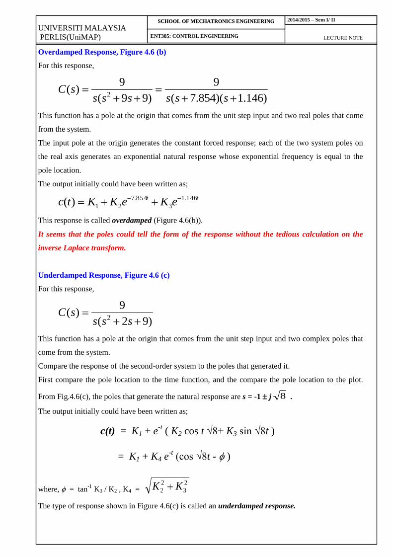
Overdamped Response, Figure 4.6 (b)

For this response,

)146.1)(854.7(

9

)99(

9)(

2

sssssssC

This function has a pole at the origin that comes from the unit step input and two real poles that come

from the system.

The input pole at the origin generates the constant forced response; each of the two system poles on

the real axis generates an exponential natural response whose exponential frequency is equal to the

pole location.

The output initially could have been written as;

tt eKeKKtc 146.1

3

854.7

21)(

This response is called overdamped (Figure 4.6(b)).

It seems that the poles could tell the form of the response without the tedious calculation on the

inverse Laplace transform.

Underdamped Response, Figure 4.6 (c)

For this response,

)92(

9)(

2

ssssC

This function has a pole at the origin that comes from the unit step input and two complex poles that

come from the system.

Compare the response of the second-order system to the poles that generated it.

First compare the pole location to the time function, and the compare the pole location to the plot.

From Fig.4.6(c), the poles that generate the natural response are s = -1 j 8 .

The output initially could have been written as;

where, = tan-1

K3 / K2 , K4 = 2

3

2

2 KK

The type of response shown in Figure 4.6(c) is called an underdamped response.

c(t) = K1 + e-t ( K2 cos t √8+ K3 sin √8t )

= K1 + K4 e-t (cos √8t - )

UNIVERSITI MALAYSIA




2014/2015 – Sem I/ II

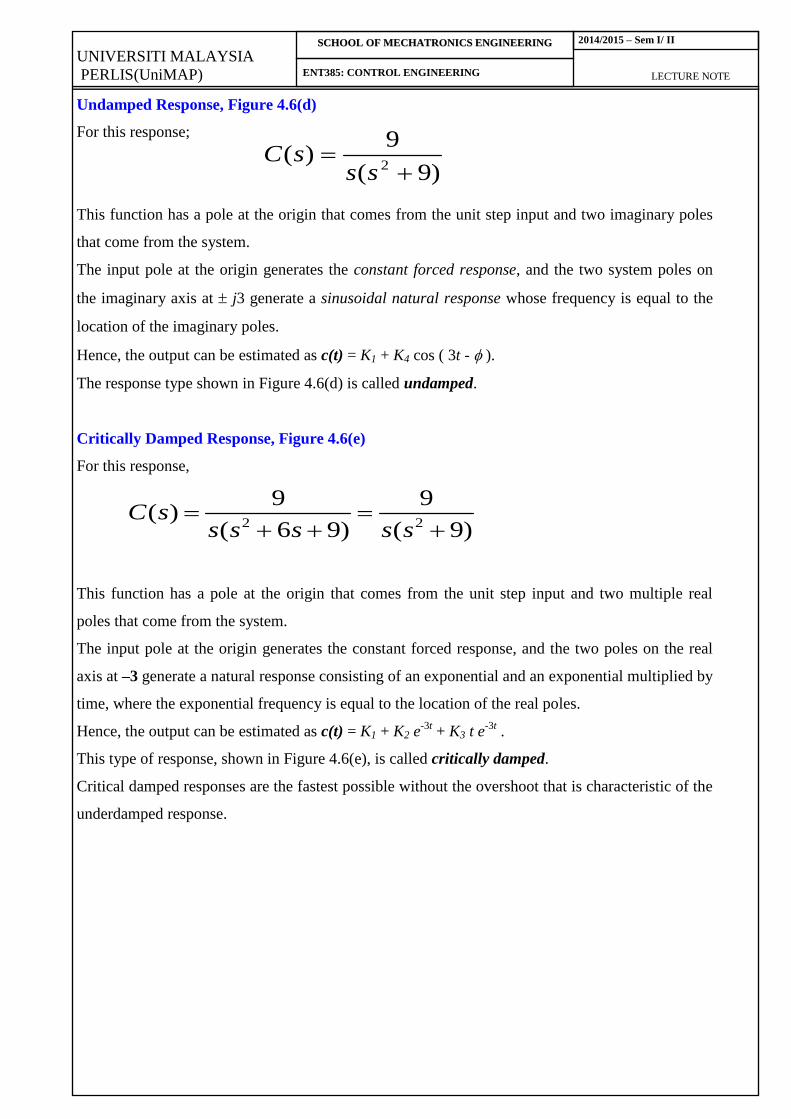
Undamped Response, Figure 4.6(d)

For this response;

This function has a pole at the origin that comes from the unit step input and two imaginary poles

that come from the system.

The input pole at the origin generates the constant forced response, and the two system poles on

the imaginary axis at j3 generate a sinusoidal natural response whose frequency is equal to the

location of the imaginary poles.

Hence, the output can be estimated as c(t) = K1 + K4 cos ( 3t - ).

The response type shown in Figure 4.6(d) is called undamped.

Critically Damped Response, Figure 4.6(e)

For this response,

)9(

9

)96(

9)(

22

ssssssC

This function has a pole at the origin that comes from the unit step input and two multiple real

poles that come from the system.

The input pole at the origin generates the constant forced response, and the two poles on the real

axis at –3 generate a natural response consisting of an exponential and an exponential multiplied by

time, where the exponential frequency is equal to the location of the real poles.

Hence, the output can be estimated as c(t) = K1 + K2 e-3t

+ K3 t e-3t

.

This type of response, shown in Figure 4.6(e), is called critically damped.

Critical damped responses are the fastest possible without the overshoot that is characteristic of the

underdamped response.

)9(

9)(

2

sssC

UNIVERSITI MALAYSIA




2014/2015 – Sem I/ II

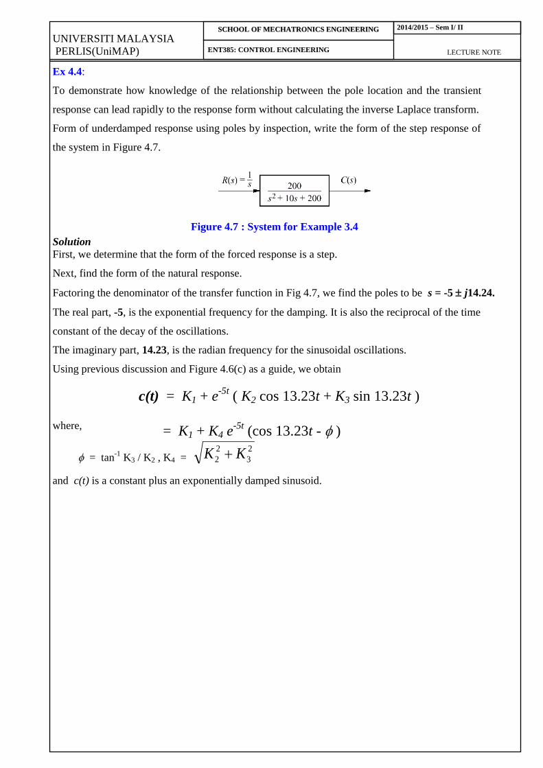
Ex 4.4:

To demonstrate how knowledge of the relationship between the pole location and the transient

response can lead rapidly to the response form without calculating the inverse Laplace transform.

Form of underdamped response using poles by inspection, write the form of the step response of

the system in Figure 4.7.

Solution

First, we determine that the form of the forced response is a step.

Next, find the form of the natural response.

Factoring the denominator of the transfer function in Fig 4.7, we find the poles to be s = -5 j14.24.

The real part, -5, is the exponential frequency for the damping. It is also the reciprocal of the time

constant of the decay of the oscillations.

The imaginary part, 14.23, is the radian frequency for the sinusoidal oscillations.

Using previous discussion and Figure 4.6(c) as a guide, we obtain

where,

= tan-1

K3 / K2 , K4 = 2

3

2

2 KK

and c(t) is a constant plus an exponentially damped sinusoid.

Figure 4.7 : System for Example 3.4

c(t) = K1 + e-5t

( K2 cos 13.23t + K3 sin 13.23t )

= K1 + K4 e-5t

(cos 13.23t - )

UNIVERSITI MALAYSIA




2014/2015 – Sem I/ II

Figure 4.6

UNIVERSITI MALAYSIA




2014/2015 – Sem I/ II

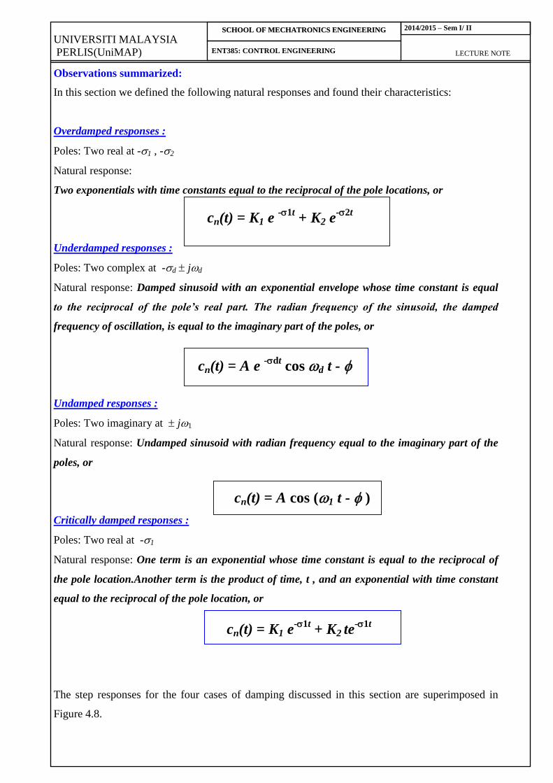
Observations summarized:

In this section we defined the following natural responses and found their characteristics:

Overdamped responses :

Poles: Two real at -1 , -2

Natural response:

Two exponentials with time constants equal to the reciprocal of the pole locations, or

Underdamped responses :

Poles: Two complex at -d jd

Natural response: Damped sinusoid with an exponential envelope whose time constant is equal

to the reciprocal of the pole’s real part. The radian frequency of the sinusoid, the damped

frequency of oscillation, is equal to the imaginary part of the poles, or

Undamped responses :

Poles: Two imaginary at j1

Natural response: Undamped sinusoid with radian frequency equal to the imaginary part of the

poles, or

Critically damped responses :

Poles: Two real at -1

Natural response: One term is an exponential whose time constant is equal to the reciprocal of

the pole location.Another term is the product of time, t , and an exponential with time constant

equal to the reciprocal of the pole location, or

The step responses for the four cases of damping discussed in this section are superimposed in

Figure 4.8.

cn(t) = K1 e -1t

+ K2 e-2t

cn(t) = A e -dt

cos d t -

cn(t) = A cos (1 t - )

cn(t) = K1 e-1t

+ K2 te-1t

UNIVERSITI MALAYSIA




2014/2015 – Sem I/ II

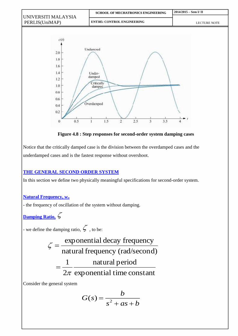
Notice that the critically damped case is the division between the overdamped cases and the

underdamped cases and is the fastest response without overshoot.

THE GENERAL SECOND ORDER SYSTEM

In this section we define two physically meaningful specifications for second-order system.

Natural Frequency, wn

- the frequency of oscillation of the system without damping.

Damping Ratio,

- we define the damping ratio, , to be:

constant timelexponentia

period natural

2

1

d)(rad/seconfrequency natural

frequencydecay lexponentia

Consider the general system

bass

bsG

2)(

Figure 4.8 : Step responses for second-order system damping cases

UNIVERSITI MALAYSIA




2014/2015 – Sem I/ II

Without damping, the poles would be on the jw axis, and the response would be an undamped

sinusoid. For the poles to be purely imaginary, a=0. Hence, by definition, the natural frequency, wn, is

the frequency of oscillation of this system. Since the poles of this system are on the jw axis at

bj ,

bwn

Hence, 2

nwb

Assuming an underdamped system, the complex poles have a real part, , equal to –a/2. The

magnitude of this value is then the exponential decay frequency described in section 4.4. Hence,

nn w

a

wradfrequencyNatural

frequencydecaylExponentia 2

sec)/(

nwa 2

Our general second-order transfer function finally looks like this:

22

2

2)(

nn

n

wsws

wsG

Solving the poles of the transfer function, G(s) yields:

12

2,1 nn wws

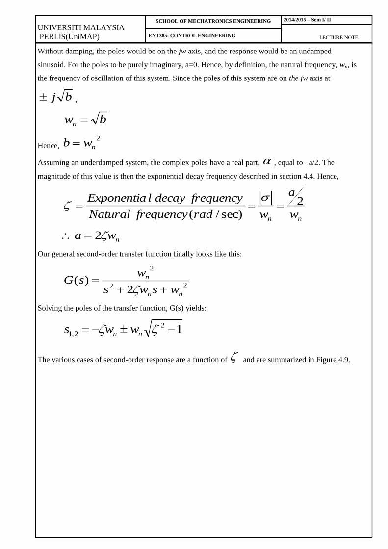
The various cases of second-order response are a function of and are summarized in Figure 4.9.

UNIVERSITI MALAYSIA




2014/2015 – Sem I/ II

Figure 4.9

UNIVERSITI MALAYSIA




2014/2015 – Sem I/ II

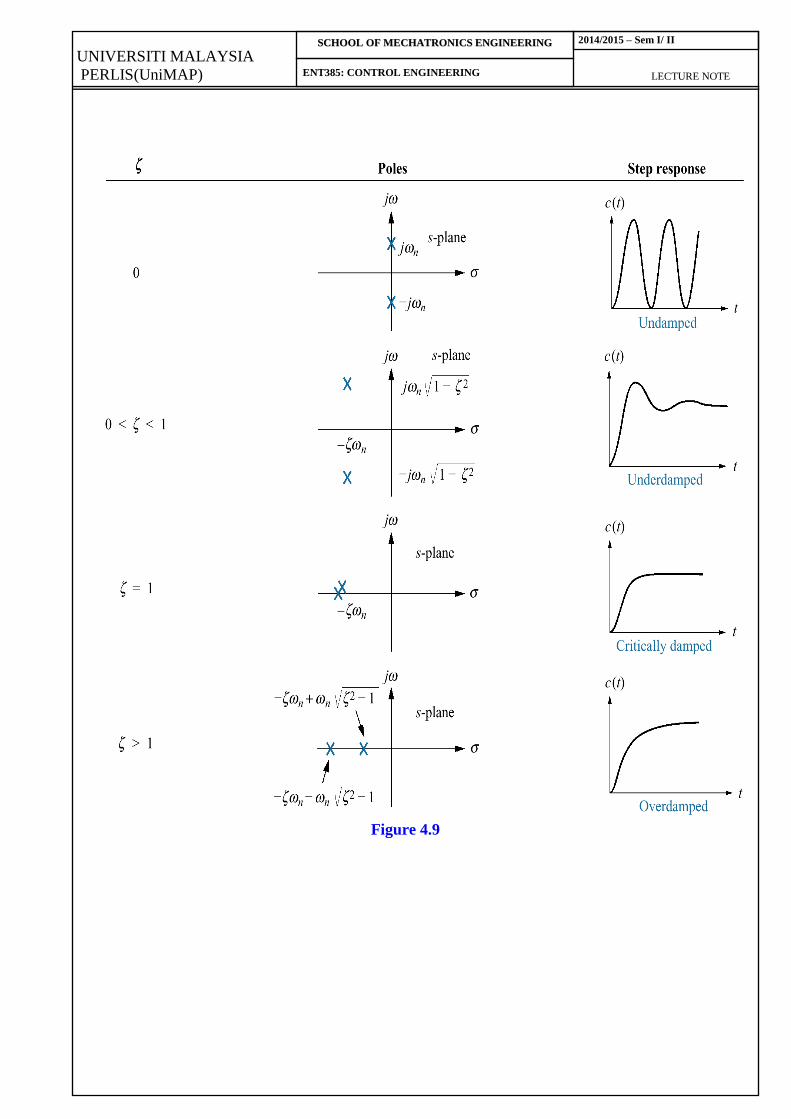
Ex 4.5

Given the transfer function as shown below, find and wn.

362.4

36)(

2

sssG

Solution

Compare with the general second-order transfer function, 22

2

2)(

nn

n

wsws

wsG

therefore,

362nw ; 6 nw and

2.42 nw ; 35.0

62

2.4

Ex 4.6

For each of the systems shown in Figure 4.10, fins the value of and give the kind of response

expected.

Figure 4.10

Answer:

a) 155.1 , overdamped response

b) 1 , critically damped response

c) 894.0 , underdamped response

UNIVERSITI MALAYSIA




2014/2015 – Sem I/ II

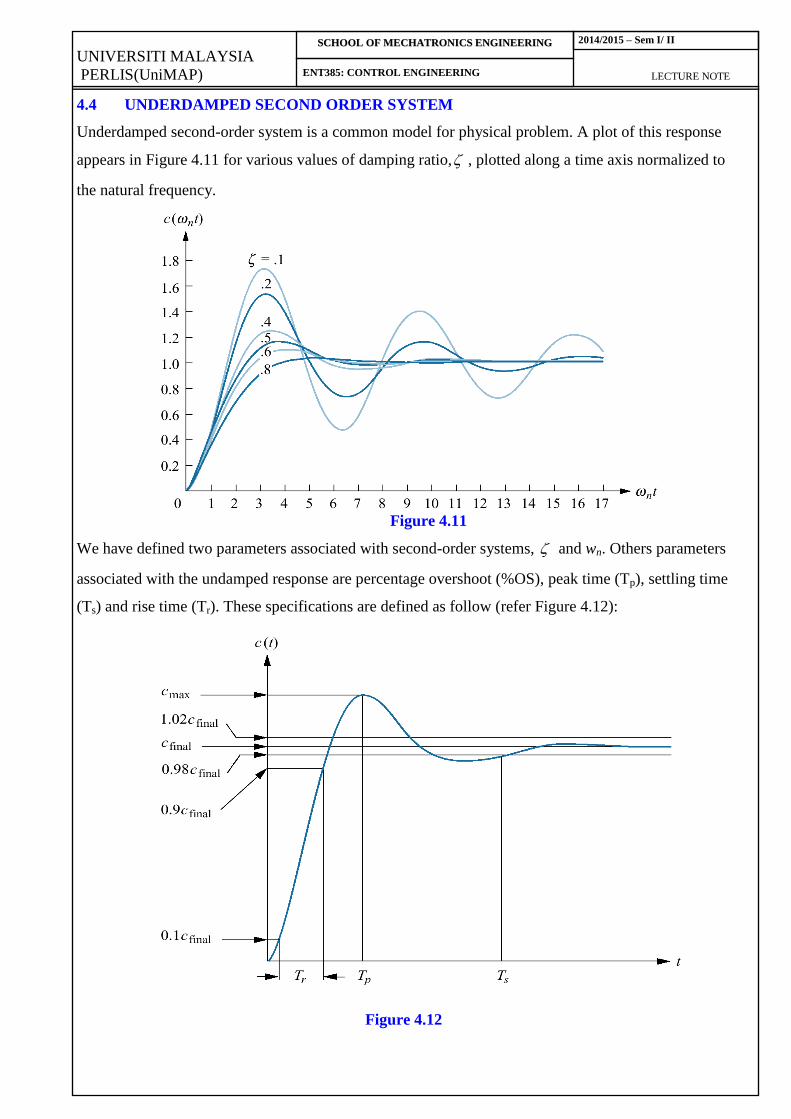
4.4 UNDERDAMPED SECOND ORDER SYSTEM

Underdamped second-order system is a common model for physical problem. A plot of this response

appears in Figure 4.11 for various values of damping ratio, , plotted along a time axis normalized to

the natural frequency.

Figure 4.11

We have defined two parameters associated with second-order systems, and wn. Others parameters

associated with the undamped response are percentage overshoot (%OS), peak time (Tp), settling time

(Ts) and rise time (Tr). These specifications are defined as follow (refer Figure 4.12):

Figure 4.12

UNIVERSITI MALAYSIA




2014/2015 – Sem I/ II

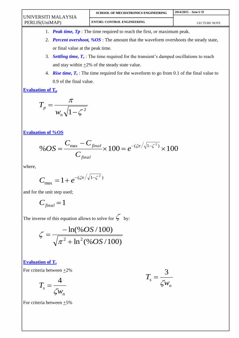
1. Peak time, Tp : The time required to reach the first, or maximum peak.

2. Percent overshoot, %OS : The amount that the waveform overshoots the steady state,

or final value at the peak time.

3. Settling time, Ts : The time required for the transient’s damped oscillations to reach

and stay within +2% of the steady state value.

4. Rise time, Tr : The time required for the waveform to go from 0.1 of the final value to

0.9 of the final value.

Evaluation of Tp

21

n

p

wT

Evaluation of %OS

100100%)1(max 2

eC

CCOS

final

final

where,

)1(

max

2

1

eC

and for the unit step used;

1finalC

The inverse of this equation allows to solve for by:

)100/(%ln

)100/ln(%

22 OS

OS

Evaluation of Ts

For criteria between +2%

n

sw

T

4

For criteria between +5%

n

sw

T

3

UNIVERSITI MALAYSIA

PERLIS (UniMAP) LECTURE NOTE



2013/2014 – Sem I/ II

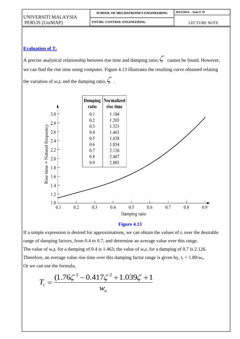
Evaluation of Tr

A precise analytical relationship between rise time and damping ratio, cannot be found. However,

we can find the rise time using computer. Figure 4.13 illustrates the resulting curve obtained relating

the variation of wntr and the damping ratio, .

Figure 4.13

If a simple expression is desired for approximations, we can obtain the values of tr over the desirable

range of damping factors, from 0.4 to 0.7, and determine an average value over this range.

The value of wntr for a damping of 0.4 is 1.463; the value of wntr for a damping of 0.7 is 2.126.

Therefore, an average value rise time over this damping factor range is given by, tr = 1.80/wn.

Or we can use the formula,

n

rw

T1039.1417.076.1( 23

UNIVERSITI MALAYSIA




2013/2014 – Sem I/ II

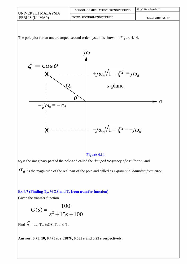
The pole plot for an underdamped second order system is shown in Figure 4.14.

Figure 4.14

wd is the imaginary part of the pole and called the damped frequency of oscillation, and

d is the magnitude of the real part of the pole and called as exponential damping frequency.

Ex 4.7 (Finding Tp, %OS and Ts from transfer function)

Given the transfer function

10015

100)(

2

sssG

Find , wn, Tp, %OS, Ts and Tr.

Answer: 0.75, 10, 0.475 s, 2.838%, 0.533 s and 0.23 s respectively.

cos

UNIVERSITI MALAYSIA




2013/2014 – Sem I/ II

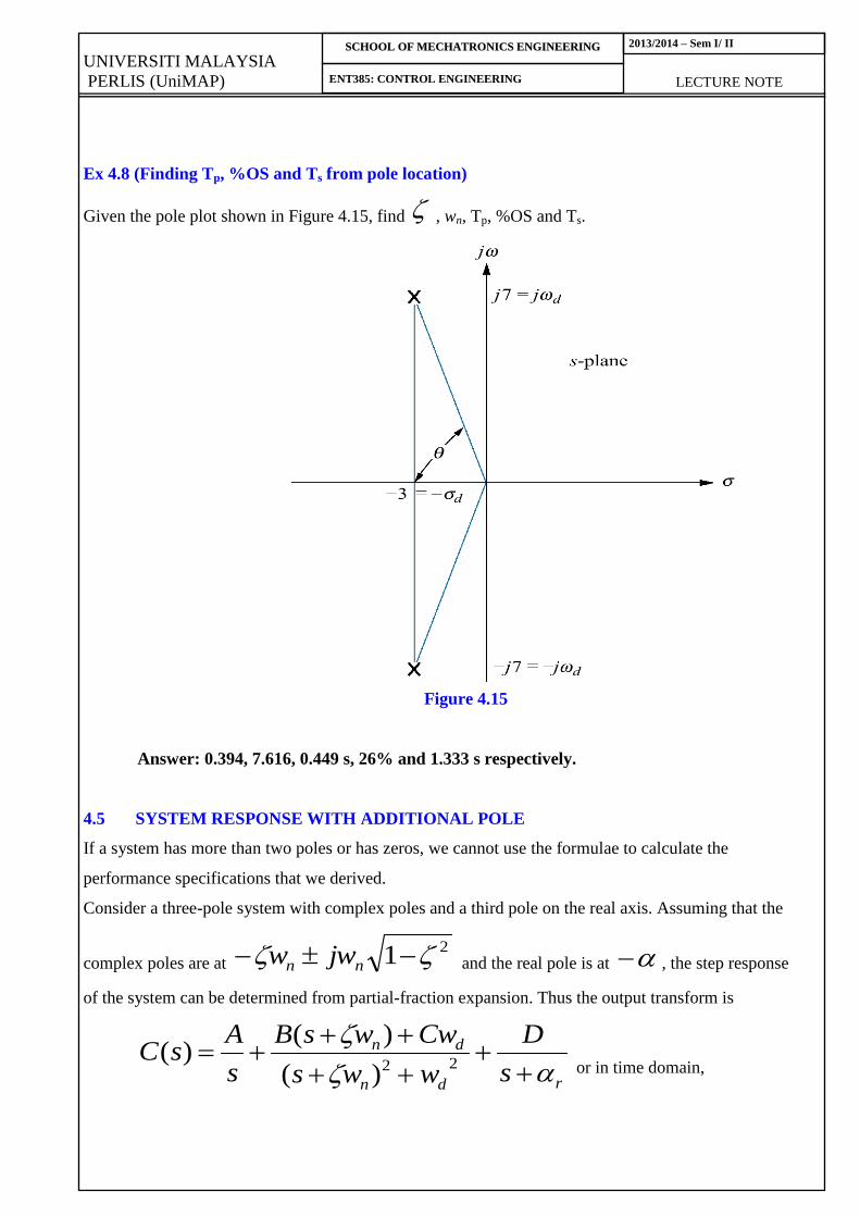
Ex 4.8 (Finding Tp, %OS and Ts from pole location)

Given the pole plot shown in Figure 4.15, find , wn, Tp, %OS and Ts.

Figure 4.15

Answer: 0.394, 7.616, 0.449 s, 26% and 1.333 s respectively.

4.5 SYSTEM RESPONSE WITH ADDITIONAL POLE

If a system has more than two poles or has zeros, we cannot use the formulae to calculate the

performance specifications that we derived.

Consider a three-pole system with complex poles and a third pole on the real axis. Assuming that the

complex poles are at 21 nn jww and the real pole is at , the step response

of the system can be determined from partial-fraction expansion. Thus the output transform is

rdn

dn

s

D

wws

CwwsB

s

AsC

22)(

)()(

or in time domain,

UNIVERSITI MALAYSIA




2013/2014 – Sem I/ II

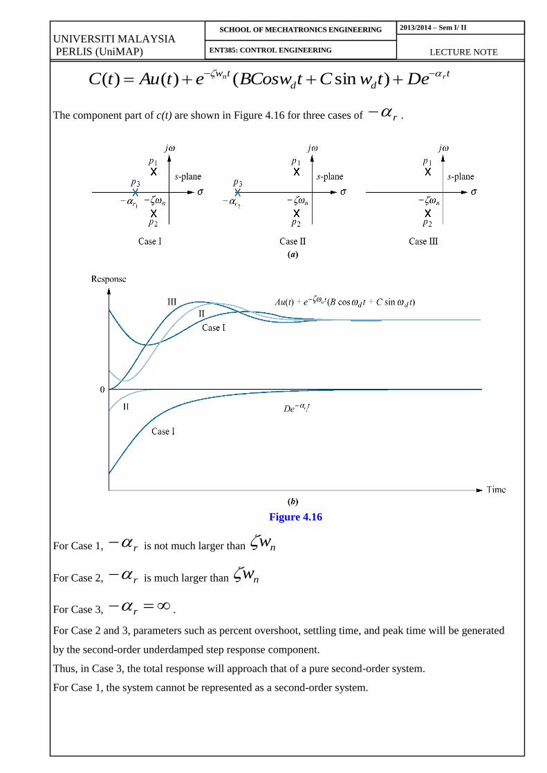
t

dd

tw rn DetwCtBCoswetAutC

)sin()()(

The component part of c(t) are shown in Figure 4.16 for three cases of r .

Figure 4.16

For Case 1, r is not much larger than nw

For Case 2, r is much larger than nw

For Case 3, r .

For Case 2 and 3, parameters such as percent overshoot, settling time, and peak time will be generated

by the second-order underdamped step response component.

Thus, in Case 3, the total response will approach that of a pure second-order system.

For Case 1, the system cannot be represented as a second-order system.

UNIVERSITI MALAYSIA




2013/2014 – Sem I/ II

Thus, if the real pole is five times farther from the dominant poles, we assume that the system is

represented by its dominant second-order pair of poles.

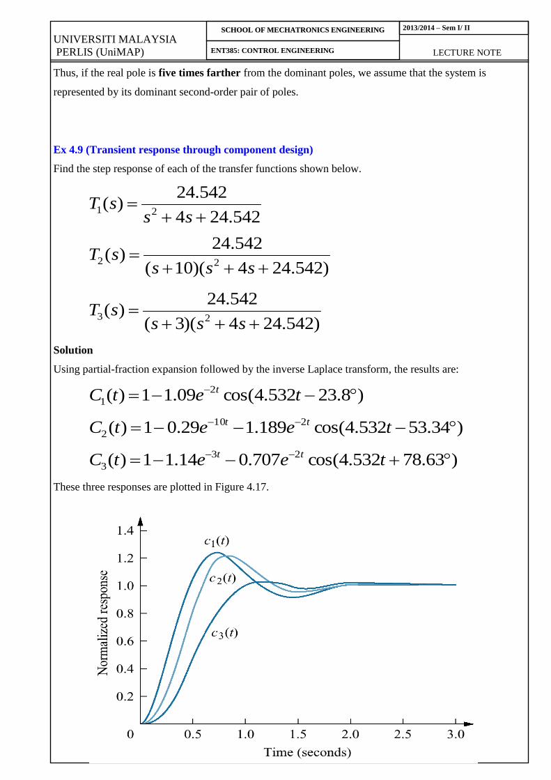
Ex 4.9 (Transient response through component design)

Find the step response of each of the transfer functions shown below.

542.244

542.24)(

21

ss

sT

)542.244)(10(

542.24)(

22

sss

sT

)542.244)(3(

542.24)(

23

sss

sT

Solution

Using partial-fraction expansion followed by the inverse Laplace transform, the results are:

)8.23532.4cos(09.11)( 2

1 tetC t

)34.53532.4cos(189.129.01)( 210

2 teetC tt

)63.78532.4cos(707.014.11)( 23

3 teetC tt

These three responses are plotted in Figure 4.17.

UNIVERSITI MALAYSIA




2013/2014 – Sem I/ II

Figure 4.17

Notice that c2(t), with its third pole at –10 and farthest from the dominant poles, is the better

approximation of c1(t).

C3(t)with a third pole close to the dominant poles, yields the most error.

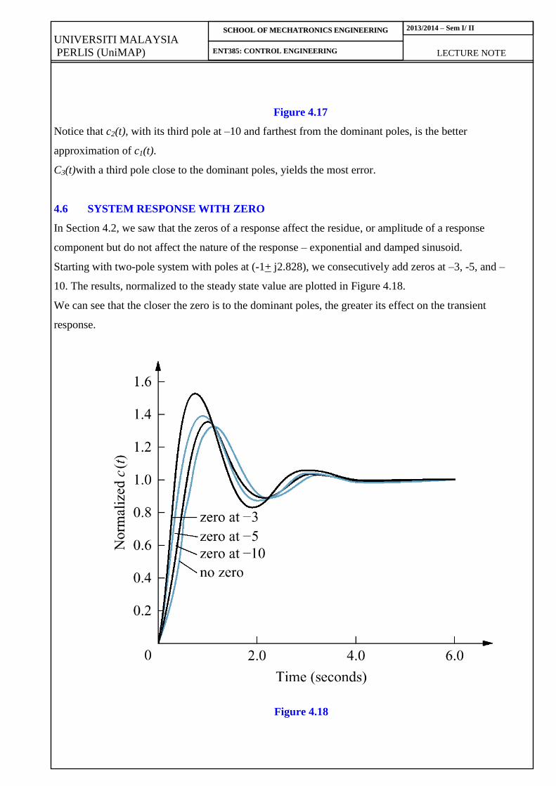
4.6 SYSTEM RESPONSE WITH ZERO

In Section 4.2, we saw that the zeros of a response affect the residue, or amplitude of a response

component but do not affect the nature of the response – exponential and damped sinusoid.

Starting with two-pole system with poles at (-1+ j2.828), we consecutively add zeros at –3, -5, and –

10. The results, normalized to the steady state value are plotted in Figure 4.18.

We can see that the closer the zero is to the dominant poles, the greater its effect on the transient

response.

Figure 4.18

chapter 4 : time response - unimap portalportal.unimap.edu.my/portal/page/portal30/lecture... ·...

Documents